On the origin of the minimal coupling rule, and on the possiblity of observing a classical, “Aharonov-Bohm-like” angular momentum

Professor Roland Winston recently reminded me of Landau’s argument in Landau and Lifshitz’s book The Classical Theory of Fields [1], which starts from the principle of the relativistic invariance of the classical action of a charged particle in the presence of classical electromagnetic fields, whence one can derive the “minimal coupling rule”, viz.,

$$\mathbf{p}\rightarrow\mathbf{p}-q\mathbf{A}$$ (1)

and also the Lorentz force law

$$\mathbf{F}=q\mathbf{E}+q\mathbf{v\times B}$$ (2)

This avoids the usual procedure of just postulating the minimal coupling rule within standard quantum mechanics, or just adding the Lorentz force law as an extra postulate to Maxwell’s equations found in most textbooks on electrodynamics. Professor Winston emphasized to me how very powerful relativistic invariance is: It puts such a powerful constraint on the form of the action that it leads inexorably to both to the minimal coupling rule and to the Lorentz force law. Since the minimal coupling rule is equivalent to the principle of local gauge invariance, it is curious that one can “derive”, in some sense, the principle of local gauge invarance from Lorentz invariance using Landau’s argument. This suggests that, in some hidden way, the symmetries of spacetime are the source and origin of the local gauge principle, and therefore of all the forces of nature.

Let us first start with the Feynman path-integral formulation of quantum mechanics, which states that the probability amplitude of a particle to go from point $a$ to point $b$ is the sum over all the probability amplitudes for all possible paths joining points $a$ and $b$, i.e.,

$$\left\langle b\right.\left|a\right\rangle=\sum_{n}{\exp\left(\frac{iS[\text{path }n]}{\hbar}\right)}$$ (3)

where the action, which is a functional, i.e., a function-like mathematical object, which assigns a numerical value to an argument that is another function $x_{n}(t)~{}$that specifies the path $n$

$$S[\text{path }n]\equiv S[x_{n}(t)]$$ (4)

where

$$S[\text{path }n]\text{=}\left.\int_{a}^{b}L(x,\dot{x})dt\right|_{\text{path }n}$$ (5)

where

$$L(x,\dot{x})=T(\dot{x})-V(x)=\frac{1}{2}m\dot{x}^{2}-V(x)$$ (6)

is the Lagrangian evaluated along the given path $x_{n}(t)$, which need not be the classical path, but can be any path joining the two fixed points $a$ and $b$, i.e., the known starting point $a$ and the known ending point $b$ of the particle. Point $a$ is to be interpreted as the point of emission of the particle, and point $b$ is the point of detection of the particle.

The classical path is the one that extremizes the action, but Feynman pointed out that in quantum mechanics, one must generalize the action to a sum over paths, in order to include the contribution from all possible paths, and not just the one (i.e., the classical path) that extremizes the action. The superposition principle of quantum mechanics is embodied in this sum. In fact, all possible paths must have the exactly equal weighting specified by the phase-factor formula (3) in order to recover the standard Schrödinger-equation description for the evolution of the wavefunction. Extremizing the action is equivalent, physically speaking, to the method of constructive interference of Huygens’ secondary wavelets; mathematically speaking, extremizing the action is equivalent to the method of stationary phase.

It is clear from (3) that the meaning of the action $S[$path $n]$ (divided by the reduced Planck’s constant) is that it is the quantum mechanical phase $\phi$ which is accumulated by the particle upon tranversing the path $n$ from point $a$ to point $b$, i.e.,

$$\left.\phi[\text{path }n]\right|_{a}^{b}=\frac{\left.S[\text{path }n]\right|_{a}^{b}}{\hbar}$$ (7)

Dirac, and later Feynman, introduced as a postulate that a particle with a charge $q$ moving through a space filled by a vector potential $\mathbf{A}$ will acquire an additional phase factor over and beyond the usual phase factor arising from the action (5) for a neutral particle with mass $m$ (5). This extra phase factor is given by

$$\exp(i\phi_{\text{charge}})=\exp\left(i\frac{q}{\hbar}\int_{a}^{b}\mathbf{A\cdot}d\mathbf{l}\right)$$ (8)

where $d\mathbf{l}$ is a line element of the path taken by the charge. This is equivalent to postulating that the Lagrangian has an extra piece $L_{\text{charge}}$ in addition to (6), viz.,

$$L_{\text{charge}}=q\mathbf{A\cdot v}$$ (9)

where $q$ is the charge of the particle, $\mathbf{v}$ is the three-velocity of the charged particle moving through a region of space with a vector potential $\mathbf{A}$. From the extra piece of the Lagrangian (9), it follows that, at the quantum level of description, there will exist an extra piece of “charged” momentum gotten by taking a partial derivative of the Lagrangian with respect to the velocity $\mathbf{\dot{x}=v}$

$$\mathbf{p}_{\text{charge}}=\frac{\partial L_{\text{charge}}}{\partial\mathbf{\dot{x}}}=\frac{\partial L_{\text{charge}}}{\partial\mathbf{v}}=q\mathbf{A}$$ (10)

which we shall call this the “$q\mathbf{A}$-type” momentum, or “electromagnetic momentum”, which a particle with a charge $q$ would possess by virtue of its charged coupling to electromagnetic fields, which is in addition to the standard “$m\mathbf{v}$” momentum, or “kinetic” momentum, that a neutral particle with mass $m$ moving with a velocity $\mathbf{v}$ would possess. Note that even if the charged particle $q$ is at rest, so that its “$m\mathbf{v}$” momentum is zero, it can still possess a non-zero “$q\mathbf{A}$-type” momentum in the presence of a non-vanishing $\mathbf{A}$ field, such as that arising from the flux inside an infinitely long solenoid in the Aharonov-Bohm effect.

But where does this extra piece of the Lagrangian $q\mathbf{A\cdot v}$ come from? Why does the vector potential appear here instead of the more “physically real” electric or magnetic fields? What happened to gauge invariance here? Does the extra piece of the Lagrangian $q\mathbf{A\cdot v}$ exist at the classical level of description of the motion of a classical charged particle in the presence of classical electromagnetic fields, as well as at the quantum level?

In order to answer these questions, let’s return to an entirely classical description of the motion of a charged particle in a classical electromagnetic field, and let’s follow Landau’s method of constraining the form of the classical action for the charged particle’s motion based on the principle of Lorentz invariance, following Professor Winston’s suggestion. Let’s first generalize (5) to its relativistic form

$$S[\text{path }\gamma]\text{=}\left.\int_{a}^{b}L(x^{\mu},\frac{dx^{\mu}}{d\tau})d\tau\right|_{\text{path }\gamma}$$ (11)

where $x^{\mu}$ is the four-vector position of a classical particle and

$$v^{\mu}=\frac{dx^{\mu}}{d\tau}$$ (12)

is the four-velocity of the particle, where the spacetime path $\gamma$ is that of the classical trajectory of a charged particle from the starting spacetime point $a$ to the ending spacetime point $b$ of the trajectory in spacetime, and where $d\tau$ is the infinitesimal increment of proper time of the particle along its trajectory. Landau demanded that the form of the action $S$ must be relativistically invariant under all possible Lorentz transformations, i.e., it must have the form of a four-scalar, or invariant, in spacetime.

Now let the particle have both a mass $m$ and a charge $q$. Then the total action (where we omit the limits of integration and suppress the path specification as being understood) will be the sum of two parts

$$S=S_{\text{mass}}+S_{\text{charge}}$$ (13)

where the first term must have the relativistically invariant form

$$S_{\text{mass}}=mc^{2}\int d\tau=mc\int ds$$ (14)

where $m$ is the rest mass of the particle, where $c$ is the speed of light, and where the invariant interval $ds$ in general relativity is defined through a quadratic form via the metric tensor $g_{\mu\nu}$

$$ds^{2}=g_{\mu\nu}dx^{\mu}dx^{\nu}$$ (15)

(We shall use Einstein’s summation convention for repeated spacetime indices, i.e., for Greek-letter spacetime indices running from 0 to 3, with a metric signature of ($-$1, +1, +1, +1)). In the case of special relativity

$$ds^{2}=\eta_{\mu\nu}dx^{\mu}dx^{\nu}$$ (16)

where the Minkowski tensor is the diagonal tensor defined as follows:

$$\eta_{\mu\nu}=\text{diag}\left(-1,+1,+1,+1\right)$$ (17)

so that using Cartesian coordinates

$$ds^{2}=-c^{2}dt^{2}+dx^{2}+dy^{2}+dz^{2}$$

Note that in special relativity, $S_{\text{mass}}$ is manifestly a Lorentz scalar, and is therefore relativistically invariant. Furthermore, it has the units of the product of energy and time, i.e., the units of Planck’s constant, so that $S_{\text{mass}}/\hbar$ is a dimensionless quantity, which is consistent with the quantum phase $\phi=S_{\text{mass}}/\hbar$ being dimensionless. Note that even if the particle were to be neutral, i.e., with $q=0$, but $m\neq 0$, it still must have a contribution $S_{\text{mass}}$ to its action. This term, when extremized using the standard variational principle $\delta S=0$, yields, in the non-relativistic limit, Newton’s second law of motion via the standard Euler-Lagrange equations of motion. Thus one recovers the standard nonrelativistic form of classical mechanics.

Next, let’s consider all the possible forms for $S_{\text{charge}}$ that are allowed by relativistic invariance. The action $S_{\text{charge}}$ at the classical level represents a measure of the coupling of the motion of a charged particle to all classical electromagnetic fields, and at the quantum level it becomes the phase change of the particle arising from the interaction of a moving charge with these fields. The motion of the charged particle is described by the four-vector

$$v^{\mu}=\frac{dx^{\mu}}{d\tau}=\text{particle's four-velocity}$$ (18)

In a proper-time increment $d\tau$, the particle is displaced by the four-vector

$$dx^{\mu}=v^{\mu}d\tau=\text{particle's four-displacement}$$ (19)

We seek an action $S_{\text{charge}}$ which satisfies the linearity requirement

$$dS_{\text{charge}}\propto dx^{\mu}$$ (20)

for infinitesimal increments of $dx^{\mu}$ in the presence of electromagnetic fields. This requirement follows from the fact that all “physically reasonable” fields must become uniform fields, when they are viewed on the tiny, infinitesimal length scales given by $dx^{\mu}$. Hence the action of displacing a charge in the presence of such uniform fields by an infinitesimal amount $dx^{\mu}$ must be linear in $dx^{\mu}$, with the exception of the gravitational field, for which a uniform gravitational field, such as the $\mathbf{g}$ field of the Earth, acting on a particle within an infinitesimally small region of spacetime, can always be transformed away by the equivalence principle. Therefore, instead of a linear dependence on $dx^{\mu}$ given by $dS_{\text{charge}}\propto dx^{\mu}$, one must use for the action of gravity on a particle the square-root of the quadratic form given by

$$dS_{\text{mass}}\propto\sqrt{g_{\mu\nu}dx^{\mu}dx^{\nu}}$$ (21)

Note the contrast between the non-analytic nature of the square-root function in (21), versus the analytic nature of the linear function in (20). (I thank Steve Minter for pointing out this imporant difference to me).

Furthermore, we shall require that the action

$$dS_{\text{charge}}\propto q$$ (22)

be directly proportional to the size and the sign of the charge of the particle which is interacting with an electromagnetic field. We shall assume here that the charge $q$ is a Lorentz invariant quantity. It follows that

$$dS_{\text{charge}}\propto qdx^{\mu}$$ (23)

However, we note that $dS_{\text{charge}}$ transforms as a four-scalar, whereas $qdx^{\mu}$ transforms as a four-vector, under Lorentz transformations. The only way that this can happen is if we contract $dx^{\mu}$ with some other four-vector. The only four-vector that one can reasonably associate with electromagnetic fields is the vector potential $A_{\mu}$. This suggests that we try

$$dS_{\text{charge}}=qA_{\mu}dx^{\mu}$$ (24)

as an Ansatz for the action of electromagnetic fields acting on a charge $q$. This trial solution for $dS_{\text{charge}}$ has the right dimensions (we use SI units here).

There remains a sign ambiguity in this Ansatz, however, which is resolved by taking the nonrelativistic limit, in which case one gets

$$dS_{\text{charge}}=+q\mathbf{A\cdot v}dt=L_{\text{charge}}dt$$ (25)

which has the correct sign given the usual sign conventions for charges, currents, and magnetic fields (i.e., positive charges as the carriers of positive electrical currents are the sources of magnetic fields via the usual right-hand rule), and given Landau and Lifshitz’s metric signature of ($-$1, +1, +1, +1). Thus one recovers the non-relativistic charge Lagrangian of the form (9) with the correct sign, and the minimal coupling rule (1) also with the correct sign. One also recovers the Lorentz force law (2) with the correct sign.

It follows that, at the classical level of description, the non-relativistic limit (25) of Landau’s relativistic classical action (24) leads to the conclusion that the charge $q$ must have an extra piece of classical “electromagnetic” momentum

$$\mathbf{p}_{\text{charge}}=\frac{\partial L_{\text{charge}}}{\partial\mathbf{\dot{x}}}=\frac{\partial L_{\text{charge}}}{\partial\mathbf{v}}=q\mathbf{A}$$ (26)

or a “$q\mathbf{A}$-type” momentum, in addition to the usual, classical “$m\mathbf{v}$” momentum of a neutral particle with mass $m$, whenever and wherever a classical charge $q$ exists in the presence of a non-vanishing classical vector potential $\mathbf{A}$. A classical charged particle possesses this extra piece of momentum by virtue of its charged coupling to electromagnetic fields. It should be emphasized that this extra piece of momentum $\mathbf{p}_{\text{charge}}=q\mathbf{A}$ exists in the classical problem of the motion of the charge $q$, and not only in the quantum problem of the motion of $q$.

Luis Martinez then asked: Why can’t one perform a gauge transformation on the vector potential $\mathbf{A}$ so that it is zero at all points in space, i.e.,

$$\mathbf{p}_{\text{charge}}=q\mathbf{A=0}$$ (27)

everywhere? For it is always possible to choose a gauge transformation such that at every point in space

$$\mathbf{A\rightarrow A+\nabla}\chi=\mathbf{0}$$ (28)

by an appropriate choice of the arbitrary scalar function $\chi$ at each point in space. Then there would never exist any such thing as a “$q\mathbf{A}$ -type” or an “electromagnetic” momentum of the charge $q$, since it can always be transformed away.

However, as in the quantum Aharonov-Bohm effect, whenever there is a $closed$ curve $C$ that encloses a solenoid with nonvanishing magnetic flux within it, then, by Stokes’s theorem,

$$\oint_{C}\mathbf{A\cdot}d\mathbf{l}=\iint_{S\left(C\right)}\left(\mathbf{\nabla\times A}\right)\mathbf{\cdot}d\mathbf{S=}\iint_{S\left(C\right)}\mathbf{B\cdot}d\mathbf{S}=\Phi_{\text{enc}}\neq 0$$ (29)

which cannot be transformed away by any gauge transformation, since $\Phi_{\text{enc}}$ is a gauge-invariant quantity. Note that this argument holds at both the classical and quantum levels of description of the motion of a charge $q$.

One may then ask: Why not try coupling the charge directly to the more “physically real” electric and magnetic fields via the electromagnetic field tensor [2]

$$F_{\mu\nu}=\frac{\partial A_{\mu}}{\partial x^{\nu}}-\frac{\partial A_{\nu}}{\partial x^{\mu}}$$ (30)

which has the advantage of being manifestly gauge invariant? For example, one might try

$$dS_{\text{charge}}^{\prime}=qF_{\mu\nu}dx^{\mu}dx^{\nu}$$ (31)

The problem with this alternative “trial” four-scalar solution is two-fold: (1) $dS_{\text{charge}}^{\prime}\propto dx^{\mu}dx^{\nu}$ is quadratic in $dx^{\mu}dx^{\nu}$, and therefore violates the linearity requirement (20); (2) $F_{\mu\nu}$ is antisymmetric in the exchange of the two indices $\mu$ and $\nu$, but $dx^{\mu}dx^{\nu}$ is symmetric. Hence by symmetry

$$dS_{\text{charge}}^{\prime}=qF_{\mu\nu}dx^{\mu}dx^{\nu}=0$$ (32)

Hence it is natural to call Landau’s trial solution (24) the “minimal coupling rule”, in that it is the minimum possible coupling to EM fields (i.e., a coupling of the charge to the field that is linear, and therefore the lowest possible order of coupling, to the vector potential $\mathbf{A}$, and a coupling that is also linear, and therefore the lowest possible order of coupling, to the charge $q$) that is permitted by relativity. It can be shown that the usual “minimal coupling rule” (1) then follows from (24) in the non-relativistic limit in the Hamiltonian formulation of quantum mechanics.

Now we are in a position to justify the “Huygens’ construction” shown in Figure 1, in which we assume that a single electron is moving non-relativistically in a magnetic field.

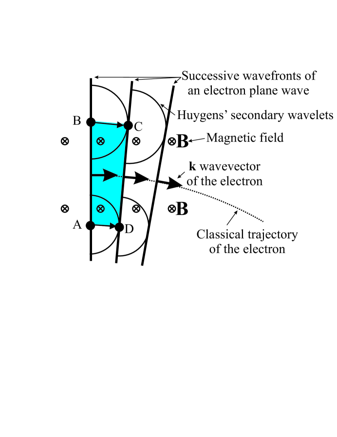
Figure 1: Huygens’ construction applied to an electron plane wave propagating towards the right in a magnetic field $\mathbf{B}$, which points into the page. The secondary wavelets emitted from points $A\$and $B$ on the primary wavefront will suffer a relative Aharonov-Bohm phase shift arising from the magnetic flux enclosed in the trapezoid $ABCD$. This phase shift leads to the bending of the normals to the successive wavefronts, and leads to a curved classical trajectory.

When the electron wave propagates through a space in which there exists a uniform magnetic field $\mathbf{B}$ that is applied perpendicularly to the electron’s initial momentum, as in Figure 1, there will arise an Aharonov-Bohm phase shift between the two secondary Huygens wavelets emanating from points $A$ and $B$ and arriving at points $C$ and $D$, which is given by

$$\Delta\phi=\frac{1}{\hbar}\oint_{ABCD}\mathbf{A}\cdot d\mathbf{l}=\frac{1}{\hbar}e\Phi_{\text{enc}}$$ (33)

where $e$ is the electron charge, $\mathbf{A}$ is the vector potential, and $\Phi_{\text{enc}}$ is the flux enclosed within the trapezoid $ABCD$ in Figure 1.

The Aharonov-Bohm phase shift arises here because the electron, as it moves from $A$ to $D$, accumulates the Dirac phase

$$\Delta\phi_{AD}=\frac{1}{\hbar}\int_{A}^{D}e\mathbf{A}\cdot d\mathbf{l}$$ (34)

and as it moves from $B$ to $C$, it accumulates the Dirac phase

$$\Delta\phi_{BC}=\frac{1}{\hbar}\int_{B}^{C}e\mathbf{A}\cdot d\mathbf{l}$$ (35)

The difference between these two Dirac phases will then be given by the closed-path integral (33)

$$\Phi_{\text{enc}}=\oint_{ABCD}\mathbf{A}\cdot d\mathbf{l=}\iint_{S\left(ABCD\right)}\left(\mathbf{\nabla\times A}\right)\cdot d\mathbf{S=}\iint_{S\left(ABCD\right)}\mathbf{B}\cdot d\mathbf{S}$$ (36)

which is a manifestly gauge invariant quantity, namely, the enclosed magnetic flux $\Phi_{\text{enc}}$. It can then be shown that the resulting “tilting” of the wavefronts or phase fronts shown in Figure 1 leads to the Lorentz force and a classical cyclotron orbit.

From the above analysis, it is clear that, in addition to the usual “$m\mathbf{v}$” momentum (or “kinetic momentum”) that a neutral particle with mass $m$ would have due its motion through space with a velocity $\mathbf{v}$, a charged particle with a charge $q$ in the field of a vector potential $\mathbf{A}$ will acquire an extra piece of “electromagnetic momentum” due its charge, which is given by

$$\mathbf{p}_{\text{charge}}=q\mathbf{A}$$ (37)

even if the charge $q$ is at rest and has no “$m\mathbf{v}$” momentum. This “$q\mathbf{A}$-type” momentum exists at both the classical level of description (via the Landau invariance argument) and at the quantum level of description (via the Feynman–Dirac–Aharonov-Bohm argument).

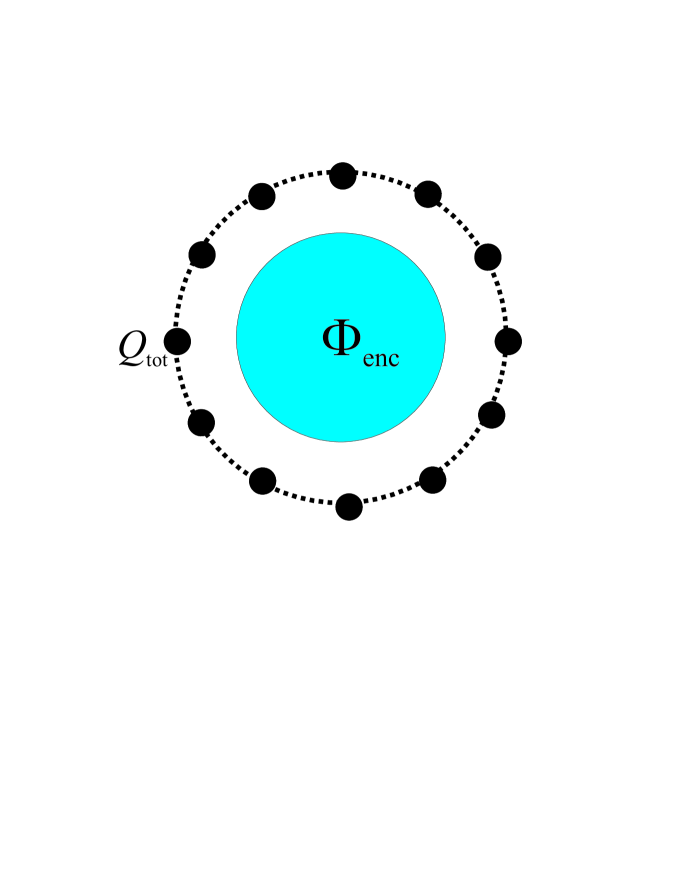
Figure 2: A “lumpy” charged ring of radius $r$ with a total charge of $Q_{\text{tot}}$ consisting of a uniform distribution of equally charged conducting spheres (in solid black) with insulation (in dashed black) separating them, forms the rotating member of a torsional pendulum. This “lumpy” ring of charges $Q_{\text{tot}}$ is placed around an infinitely long solenoid containing a flux $\Phi_{\text{enc}}$ (in blue). The electromagnetic angular momentum of this system is given by the charge-flux product $Q_{\text{tot}}\Phi_{\text{enc}}$ divided by $2\pi$, even when the charges $Q_{\text{tot}}$ are at rest. When the charge $Q_{\text{tot}}$ is suddenly discharged and disappears into the ground, the electromagnetic angular momentum $Q_{\text{tot}}\Phi_{\text{enc}}/2\pi$ will suddenly disappear, and the ring must undergo an angular recoil due to the conservation of angular momentum, and must start torsionally oscillating around the axis of the solenoid.

However, a manifestly gauge-invariant result, even at the purely classical level, can be gotten by considering a system with angular momentum in a circularly symmetric configuration, as illustrated in Figure 2, where there is a “lumpy” charge distribution, which is similar to the configuration used in “Feynman’s paradox” [3]. For then

$$\oint_{C}\mathbf{p}_{\text{charge}}\cdot d\mathbf{l} = \oint_{C}q\mathbf{A}\cdot d\mathbf{l=}$$

$$\left\langle p_{\text{charge}}\right\rangle\cdot 2\pi r = Q_{\text{tot}}\Phi_{\text{enc}}$$ (38)

$$\therefore L_{\text{charge}}=\frac{1}{2\pi}Q_{\text{tot}}\Phi_{\text{enc}}$$ (39)

where $C$ is a circle of radius $r$, where $Q_{\text{tot}}$ is the total charge, which is the sum of all the discrete charges distributed around the ring, and where $\Phi_{\text{enc}}$ is the flux enclosed by the “lumpy” charged ring. Here $\left\langle p_{\text{charge}}\right\rangle$ denotes the average of the magnitude of $\mathbf{p}_{\text{charge}}$ over the ring, and

$$\oint_{C}q\mathbf{A}\cdot d\mathbf{l}=Q_{\text{tot}}\left\langle\oint_{C}\mathbf{A}\cdot d\mathbf{l}\right\rangle\mathbf{=}Q_{\text{tot}}\Phi_{\text{enc}}$$ (40)

denotes an average over the “lumpy” charge distribution of the quantity $q\mathbf{A}$, as if there were a smooth, continuous, uniform distribution of bound charges frozen inside an insulating ring, in a continuum model of the “lumpy” charge ring.

The classical expression

$$L_{\text{charge}}=\frac{1}{2\pi}Q_{\text{tot}}\Phi_{\text{enc}}$$ (41)

obtained in (39) is in fact the same as that for the Aharonov-Bohm angular momentum at the quantum level, when one substitutes $Q_{\text{tot}}=e$ for the charge of a single, completely delocalized electron, which possesses a perfect quantum phase coherence around the ring. Note, however, that there is no requirement in the classical case for the discrete, “lumpy” charge distribution illustrated in Figure 2 to possess a single, coherent quantum-mechanical phase over the entire ring, such as is required in the case of the Aharonov-Bohm effect. Each macroscopic “lump” of charge may have decohered, and may have become a completely localized lump of classical matter which is at a perfect rest. Therefore one concludes that this “$q\mathbf{A}$-type” of angular momentum should also exist at the classical, macroscopic level of description, as well as at the quantum level. We shall call this classical type of angular momentum “Aharonov-Bohm-like” angular momentum.

An additional classical argument for the existence of the classical, “Aharonov-Bohm-like” angular momentum can be gotten by applying Faraday’s law of induction to Figure 2. Suppose that one were to increase the flux from zero inside the solenoid linearly with time by ramping up the current flowing through its coils. Then by Faraday’s law

$$\oint_{C}\mathbf{E}\cdot d\mathbf{l=-}\frac{d\Phi_{\text{enc}}}{dt}$$ (42)

Therefore the magnitude of the resulting azimuthal electric field $E$ evaluated on the circle of radius $r$ will be given by

$$E\cdot 2\pi r\mathbf{=}\frac{d\Phi_{\text{enc}}}{dt}$$ (43)

This will lead to a torque $\tau$ on the distribution of charges on the “lumpy” ring around its axis with a magnitude

$$\tau=Fr=(Q_{\text{tot}}E)r\mathbf{=}\frac{Q_{\text{tot}}}{2\pi}\frac{d\Phi_{\text{enc}}}{dt}$$ (44)

Integrating the torque over time to obtain the electromagnetic angular momentum $L_{\text{charge}}$ of the “lumpy” charged ring, one finds that

$$L_{\text{charge}}=\int\tau dt=\frac{1}{2\pi}Q_{\text{tot}}\Phi_{\text{enc}}$$ (45)

in agreement with (41). Note that this Faraday-law argument holds at the classical level.

This suggests that there may exist manifestations of “Aharonov-Bohm-like” nonlocality in classical experiments, whenever the charge $Q_{\text{tot}}$ exists in a disjoint region of space from the flux $\Phi_{\text{enc}}$. Ultimately, we should test this idea out experimentally in a Tonomura-type experiment, where the space which contains the “lumpy” circular ring of distributed charges that sum to a total charge $Q_{\text{tot}}$, and the space which contains the enclosed magnetic flux $\Phi_{enc}$, are separated into two mutually exclusive regions, such as the two separated regions of space within two linked tori.

However, we should approach this final Tonomura-type experiment in stages. In a first experiment, there would be no attempt to separate between the regions of the electric fields of $Q_{\text{tot}}$ and of the magnetic fields of $\Phi_{\text{enc}}$, so that the recoil can be explained entirely based on the classical torque arising from the Lorentz force acting on the discharging currents along the spokes of a charged wheel patterned after Figure 2 [4]. The solenoid of Figure 2 would be replaced by a permanent magnet with exposed pole faces in this first experiment. Then in the second experiment we could attempt to shield the discharge currents by using adjacent ground planes in a microstrip configuration, so that the Lorentz force on the discharging currents in the spokes of the wheel is cancelled out by the Lorentz force on the image-charge counter-currents in the ground plane. Finally, in the third experiment, we could use both ground planes and mu-metal shields in conjunction with a toroidal configuration of the magnetic flux trapped inside a high permeability metallic path, in an attempt to separate the electric and magnetic fields more or less completely into two mutually exclusive regions of space. All of these macroscopic, classical experiments could be done at room temperature.

References

- [1] L.D. Landau and E.M. Lifshitz, The Classical Theory of Fields, 4th edition: Volume 2 (Course of Theoretical Physics Series; Butterworth-Heinemann, Oxford, 2000).
- [2] Another reason for using the vector potential instead of the electromagnetic field tensor in the formulating the action is that has four spacetime components, whereas has six components. Hence one can contract the four components of with the four components of the infinitesimal to obtain a four-scalar , but there is no way to do this using the six components of .
- [3] R.P. Feynman, R.B. Leighton, and M. Sands, The Feynman Lecttures on Physics (Addison-Wesley, Reading, MA, 1964), Volume II, Section 17-4.
-
[4]
Imagine that the charged, conducting spheres in
Figure 2 were connected via radial wires to a charged central conductor,
which acts as the axle of a “lumpy” charged wheel of radius of a torsional pendulum. These radial wires can
then function as the spokes of the wheel. Moreover, imagine that the
solenoid of Figure 2 were to be replaced by a permanent magnet whose radius
is also , and whose pole face is concentrically placed in close proximity
underneath the wheel, but not touching it, so that the wheel can turn
freely. As a result, there will be a small gap through which the vertical,
uniform magnetic induction of the magnet will be applied to each spoke
of the wheel. Now let each sphere initially contain a charge . When the
central conductor is suddenly connected to ground at , a discharging
pulse of charge will travel radially with some velocity along each
spoke of the wheel in the presence of towards the grounded central axis,
so that there will be an azimuthal component of the Lorentz force of strength
acting upon each spoke. Dividing a given spoke into infinitesimal segments of length , the torque per spoke exerted on the central axle of the wheel will be given by(46)
The angular momentum imparted to the wheel per spoke by the torque during the discharge will therefore be given by(47)
where is the velocity of the pulse of charge moving along a given spoke, and where is the magnetic flux enclosed by the wheel of radius . Summing over all the charges on the wheel, one obtains that the total final (recoil) angular momentum of the wheel will be given by(48)
where is the total charge on the wheel. Note again that this derivation has been entirely performed at the classical level. This is in agreement with the more general classical result (41) obtained via (39).(49)