Symmetry breaking as the origin of zero-differential resistance states of a 2DEG in strong magnetic fields.

Abstract

Zero resistance differential states have been observed in two-dimensional electron gases (2DEG) subject to a magnetic field and a strong dc current. In a recent work we presented a model to describe the nonlinear transport regime of this phenomenon. From the analysis of the differential resistivity and the longitudinal voltage we predicted the formation of negative differential resistivity states, although these states are known to be unstable. Based on our model, we derive an analytical approximated expression for the Voltage-Current characteristics, that captures the main elements of the problem. The result allow us to construct an energy functional for the system. In the zero temperature limit, the system presents a quantum phase transition, with the control parameter given by the magnetic field. It is noted that above a threshold value ($B>B_{th}$), the symmetry is spontaneously broken. At sufficiently high magnetic field and low temperature the model predicts a phase with a non-vanishing permanent current; this is a novel phase that has not been observed so far.

1 Introduction

The study of non-equilibrium magnetotransport in high mobility two-dimensional electron gases (2DEG) has acquired great experimental and theoretical interest. Strong magnetoresistance oscillations (MIRO) and zero resistance states (ZRS) have been observed in high mobility
$GaAs/Al_{x}Ga_{1-x}As$ heterostructures subject to a magnetic field and to microwave radiation [2, 3]. Our current understanding of this phenomenon rests upon models that predict the existence of negative-resistance states (NRS) yielding an instability that rapidly drives the system into a ZRS [4]. Two distinct mechanisms for the generation of NRS are known, one is based in the microwave-induced impurity scattering [5, 6, 7, 8, 9, 10], while the second is linked to inelastic processes leading to a non-trivial electron distribution function [11, 12, 13].

More recently, Hall field-induced resistance oscillations (HIRO) and zero differential resistance states (ZDRS) have been observed in response to strong dc electric current excitations [14, 15, 16]. The effect of a direct dc current on electron transport can be quite dramatic leading to zero differential resistance states (ZDRS)[17]. At low temperature and above a threshold bias current the differential resistance vanishes and the longitudinal dc voltage becomes constant. Bykov et al.[17] discussed their experimental results following an approach similar to that of Andreev et al. [4]. In terms of the differential longitudinal resistivity $\rho_{xx}$ the stability condition reads

$$\rho_{xx}=\frac{\partial E_{x}}{\partial J_{x}}\geq 0\,.$$ (1)

Hence, according to the condition in Eq. (1) the 2DES is unstable at negative differential resistance. The presence of the ZDRS can be attributed to the formation of negative differential resistance states (NDRS) that yields an instability that drives the system into a ZDRS.

2 Model and results

In a recent work we presented a model [18, 19] to describe the nonlinear response to a direct dc current applied to a 2DEG in a strong magnetic field. The model incorporates the exact dynamics of two-dimensional damped electrons in the presence of arbitrarily strong magnetic and dc electric fields, while the effects of randomly distributed impurities are perturbatively added. From the analysis of the differential resistivity and the longitudinal voltage we observe the formation of negative differential resistivity states. Both the effects of elastic impurity scattering as well as those related to inelastic processes play an important role. The theoretical predictions correctly reproduce the main experimental features provided that the inelastic scattering rate obeys a $T^{2}$ temperature dependence, consistent with electron-electron interaction effects.

The more relevant results are presented here. After the current density is worked out, it splits into a Drude and an impurity induced contribution: $\mathbf{J}=\mathbf{J}^{D}+\mathbf{J}^{imp}$. The Drude contribution is given by $\mathbf{J}^{D}=n_{e}\,e\,\mathbf{v}_{d}$, where $n_{e}$ is the electron density and the drift velocity is given as

$$\mathbf{v}_{d}=\frac{e\tau}{m^{*}}\,\frac{\mathbf{E}-\omega_{c}\tau\,\mathbf{e}_{z}\times\mathbf{E}}{1+\omega_{c}^{2}\tau_{tr}^{2}}\,.$$ (2)

Here, $e_{z}$ is the unit vector normal to the plane of the system, $\omega_{c}$ is the cyclotron frequency, $m^{*}$ is the effective mass of the charge carrier, and $\tau_{tr}$ is the transport scattering time. It is important to point out that the Drude term is not added by hand; instead it explicitly appears in our formalism because the exact solution of the Schrödinger equation in the presence of magnetic an electric fields is obtained from a unitary transformation [19] that incorporates the solution of the classical equation of motion.

In the presence of elastic scattering an electron exchanges a momentum $\mathbf{q}=\mathbf{k}-\mathbf{k}^{\prime}$ with the impurity scatterers. Hence, the components of the impurity induced density current can be expressed as

$$J^{imp}_{i}=\frac{e\,\omega_{c}\,n_{imp}}{\hbar^{2}}\sum_{\mu\mu^{\prime}}\int\frac{d^{2}q}{2\pi}\left[f\left({\cal E}_{\mu,\frac{q}{2}}\right)-f\left({\cal E}_{\mu^{\prime},-\frac{q}{2}}\right)\right]G^{i}_{\mu\mu^{\prime}}\left(q\right)\,,$$ (3)

where $i=x,y$; $n_{imp}$ is the impurity density, and $f$ is the Fermi distribution function evaluated at the energies ${\cal E}_{\mu,q/2}$ and ${\cal E}_{\mu^{\prime},-q/2}$ respectively. The Landau levels are tilted by the electric field according to ${\cal E}_{\mu,k}=\hbar\omega_{c}\left(\mu+\frac{1}{2}\right)+\hbar\omega_{k}$; with $\omega_{k}=\mathbf{k}\cdot\mathbf{v}_{d}$. Notice that the $x$ component of the exchanged momentum $q_{x}=k_{x}-k_{x}^{\prime}$ is equivalent to a hopping (shifting of the guiding center) in the $y$ direction $\Delta y=l_{B}^{2}q_{x}$; with $l_{B}=\sqrt{\hbar/eB}$ the magnetic length. The function $G^{i}_{\mu\mu^{\prime}}$ in Eq. (3) is given by

$$G^{i}_{\mu\mu^{\prime}}=\left|V\left(q\right)\right|^{2}\left|D_{\mu\mu^{\prime}}\left(z_{q}\right)\right|^{2}\times\frac{q_{i}\Delta_{\mu\mu^{\prime}}+2\left|\epsilon_{ij}\right|q_{j}\omega_{c}\Gamma}{\Delta^{2}_{\mu\mu^{\prime}}+4\omega_{c}^{2}\Gamma^{2}},$$ (4)

in the previous equation $\epsilon_{i,j}$ is the 2D antisymmetric tensor, $\Delta_{\mu\mu^{\prime}}=\left[\omega_{q}+\omega_{c}\left(\mu-\mu^{\prime}\right)\right]^{2}-\omega_{c}^{2}+\Gamma^{2}$, $V(q)$ is the Fourier component of the scattering potential, and $\Gamma$ is the Landau level broadening factor. In order to take into account the known fact that the width of LLs depends on the magnetic field [20], we consider $\Gamma^{2}=\beta(2\omega_{c}/\pi\tau_{tr})$ where $\beta$ is a phenomenological parameter that takes into account the difference between the transport scattering time $\tau_{tr}$ and the quantum scattering time $\tau_{q}$. In the case of short range neutral impurities $\beta=1$. The matrix elements $D_{\mu,\nu}$ are given in terms of the associated Laguerre polynomial, see [19].

In recent work is has been reported that the temperature dependence of nonlinear oscillatory magnetoresistance in 2DEG subject to a strong dc electric field can be explained if the quantum scattering time $\tau_{q}$ incorporates a temperature dependence that is attributed to electron-electron interactions [21]. The quantum scattering rate is written as

$$\frac{1}{\tau_{q}}=\frac{1}{\tau_{imp}}+\frac{1}{\tau_{ee}}\,,\hskip 42.67912pt\frac{1}{\tau_{ee}}=\frac{\lambda\left(k_{B}T\right)^{2}}{\hbar\,E_{F}}\,,$$ (5)

the parameter $\lambda$ has to be experimentally determined, but it is a constant of the order of the unity. For short range neutral scatterers the impurity rate can be estimated as $1/\tau_{imp}=4\pi^{2}\hbar\alpha n_{imp}/m^{*}$, where $\alpha$ is related to the scattering length [9].

Let us now consider the nonlinear transport regime. In a current controlled scheme: the longitudinal density current is fixed to a constant value $J_{dc}$ and there is no transverse current, $J_{y}$. This leads to a set of two implicit equations for the density current

$$J_{x}\left(E_{x},E_{y}\right) = J_{dc}\,,$$

$$J_{y}\left(E_{x},Ey\right) = 0\,.$$ (6)

They represent two implicit equation for the unknown $E_{x}$ and $E_{y}$; the equations can be solved following a self-consistent iteration [19]. However, it is verified that for the conditions that apply in experiments and in the separated LL regions ($\omega_{c}\tau_{tr}\gg 1$), the solution of the previous equations simplify because the following conditions $E_{x}\ll E_{y}$ and $J_{x}^{imp}\ll en_{e}E_{y}/B$ are simultaneously satisfied. Hence, from the first equation in (2) it follows that the leading contribution to the Hall electric field is given by the classical result $E_{y}=BJ_{dc}/en_{e}$. Whereas the second equation in (2) yields a nonlinear $E_{x}\,-\,J_{dc}$ relation

$$E_{x}=\frac{m^{*}}{e^{2}\,n_{e}\tau_{tr}}\,J_{dc}+\frac{B}{en_{e}}\,J^{imp}_{y}\left(E_{x}\sim 0,E_{y}\sim\frac{BJ_{dc}}{en_{e}}\right)\,.$$ (7)

The expression for the impurity induced currents $J^{imp}_{y}$ is given in Eq. (3). In what follows we set $J_{dc}\equiv J_{x}$.

We had previously presented numerical results in very good agreement with the experimental ones, based in Eq. (7) [18], and in the self consistent solution of equations in (2) [19]. However in this work we point out that an approximated analytical $E_{x}-J_{x}$ relation can be obtained. As we are interested in the separated LL region the dominant effect is provided by the intra-Landau transitions. We include the following assumptions: (1) only the LL nearest to the Fermi level contribute. (2) The potential is taken as a constant $V(q)\equiv 2\pi\hbar^{2}\alpha/m^{*}$, corresponding to a short-range impurity scattering, and (3) the integrand in Eq. (3) has a dominant peak at the value $q_{max}\approx\sqrt{8\pi\,n_{e}}$, this allow us to carry out explicitly the integral over the Laguerre polynomials. After the angular integral are evaluated, a simply $E_{x}\,-\,J_{x}$ relation is obtained

$$E_{x}\,=\,C_{1}\,\frac{J_{x}}{\tau_{tr}}+\,C_{2}\,\frac{B^{3/2}}{\tau_{tr}\,J_{x}}\,\left[1-\frac{1}{\sqrt{1+\frac{C_{3}\,\tau_{tr}\,J_{x}^{2}}{B}}}\right]\,,$$ (8)

the parameters in this equation are given as

$$C_{1}=\frac{m^{*}}{e^{2}n_{e}},\hskip 14.22636pt\hskip 25.6073ptC_{2}=\hbar n_{imp}\,\alpha^{2}\left(\frac{2\pi e}{m^{*}}\right)^{3/2},\hskip 25.6073ptC_{3}=\frac{2\pi^{2}m^{*}}{e^{3}n_{e}}\,.$$ (9)

Eq. (8) depends on the a temperature through the $T$-dependence of $\tau_{tr}$. In the simplest approximation, short range impurity scatterers, we can consider that $\tau_{tr}$ is proportional to $\tau_{q}$, consequently the $T$ dependence is dictated by Eq. (5). Utilizing this assumption and the simple equation in (5) we carried out the comparison with the experimental results, observing a very good agreement. In particular the transition from positive to zero differential resistance states shows the correct dependence on the temperature [22].

In this work we shall concentrate in a simple but interesting limit, we take $T=0$ and consider the analysis of the stability of the NDRS. Therefore the transport scattering rate coincides with the impurity scattering rate: $1/\tau_{tr}=1/\tau_{imp}=4\pi^{2}\hbar\alpha n_{imp}/m^{*}$. In the region of positive differential resistivity $\rho_{xx}=\frac{\partial E_{x}}{\partial J_{x}}>0$, the relation between between $E_{x}$ and $J_{x}$ is single-valued and an homogeneous uniform electron density throughout the system is stable. On the other hand, in the region in which $\rho_{xx}$ is negative corresponding to a NDRS, the system becomes unstable. An approximated scheme (Maxwell construction) replaces the negative slope by a horizontal line, $i.e.$ a ZDRS. The real reason for the appearance of a negative slope in the $E_{x}-J_{x}$ plot is the implicit restraint of uniform electron density throughout the system. However in these regions configurations with a non uniform current distribution turn out to be the equilibrium configuration of the system. The simplest possible pattern is a domain wall: two parts of the sample carry stable density currents $J_{x1}$ and $J_{x2}$ with the same value of $E_{x}$. Hence we expect a phase transition defined by a critical iso-$B$ line, that passes through a critical point that is a point of inflection of this iso-$B$ line; so both $\frac{\partial E_{x}}{\partial J_{x}}$ and $\frac{\partial^{2}E_{x}}{\partial J_{x}^{2}}$ vanish at this point. The critical values: $E_{x}=E_{c}$, $J_{x}=J_{c}$ and $B=B_{c}$; at which these conditions are satisfied are readily determined as

$$J_{c}=\xi_{1}\frac{C_{1}}{\tau_{imp}^{2}\,C_{2}\,C_{3}^{3/2}},\hskip 22.76228ptE_{c}=\xi_{2}\frac{C_{1}^{2}}{\tau_{imp}^{3}\,C_{2}\,C_{3}^{3/2}}\,,\hskip 22.76228ptB_{c}^{1/2}=\xi_{3}\frac{C_{1}}{\tau_{imp}^{3/2}\,C_{2}\,C_{3}}\,.$$ (10)

with the values of the constants $\xi_{i}$ given by: $\xi_{1}\approx 40.7\,,\hskip 5.69046pt\xi_{2}\approx 161.9\,,\hskip 5.69046ptand\hskip 5.69046pt\,\xi_{3}\approx 20.85\,.$ Notice that the method follows similar steps those used in the analysis of the critical point of the Van der Waals equation [23].

Using Eqs. (9), and (10) we can express $J_{c}$, $E_{c}$ and $B_{c}$ is terms of the parameters of the system. In order to get an estimation we consider: $n_{e}=8\times 10^{15}m^{-2}$, $\mu=100m^{2}V/s$, $\alpha=0.1$, $n_{imp}=4.5\times 10^{11}m^{-2}$. So we obtain:

$$J_{c}\sim 0.4\,A/m\,,\hskip 28.45274ptE_{c}\sim 6.5\,V/m\,,\hskip 28.45274ptB_{c}\sim\,0.12\,T\,.$$ (11)

These values correspond to zero temperature, so are not directly comparable with the experimental ones, however the order of magnitude show a reasonable agreement [17].

We now define reduced variables

$$J_{r}=\frac{J_{x}}{J_{C}}\,,\hskip 28.45274ptE_{r}=\frac{E_{x}}{E_{C}}\,,\hskip 28.45274ptB_{r}=\frac{B}{B_{C}}\,.$$ (12)

Hence the critical point is localized at $J_{r}=E_{r}=B_{r}=1$. Using (8) and (12), we readily obtain the reduced voltage-current characteristic

$$E_{r}\,=\,0.25\,J_{r}\,+\,\frac{1.38}{J_{r}}\,B_{r}^{3/2}\,\left(1-\left[1+3.8\,\frac{J_{r}^{2}}{B_{r}}\right]^{-1/2}\right)\,,$$ (13)

which is “universal”, in the sense that it does not explicitly contains any parameter of the system.

Figure 1: (Color on line). Reduced longitudinal electric field $E_{r}$ as function of the reduced longitudinal current $J_{r}$, the values of $B_{r}$ are displayed near to each line.

Fig. 1 display a series of plots of reduced electric field $E_{r}$ as a function of the reduced longitudinal density current $J_{r}$ ; for various values of the reduced magnetic field. We clearly observe a phase transition: below the threshold $B_{r}<1$ the slope of the curve is always positive and the system is stable. On the other hand if $B_{r}>1$ and above the threshold bias current $(J_{r}>1)$ the differential resistivity becomes negative.

We can define a scalar Lyapunov functional $W[J_{r}]=\int\,d^{2}r\,w\left[J_{r}\right]$, where

$$w[J_{r}]=\int^{E_{r}}J_{r}\left[E_{r}^{\prime}\right]\,dE_{r}^{\prime}\,=\,\int^{J_{r}}J\,^{\prime}\,\frac{dE_{r}}{dJ_{r}^{\prime}}\,dJ_{r}^{\prime}\,.$$ (14)

Using Eq. (13) a simple calculations yields:

$$w[J_{r}]=0.125\,J_{r}^{2}+1.38\,B_{r}^{3/2}\left[1-\log\left\{2\left(1+\sqrt{1+3.8\,\frac{J_{r}^{2}}{B_{r}}}\right)\right\}-\left[1+3.8\,\frac{J_{r}^{2}}{B_{r}}\right]^{-1/2}\right]\,.$$ (15)

One can show that $W[J_{r}]$ is a Lyapunov functional, $i.e.$ a non-increasing function of time, so its minima are stable steady states. To the expression for $w[J_{r}]$ in Eq. (15) one should add a field (current) derivative contribution of the form $\lambda|\nabla\cdot\mathbf{E}|^{2}$, where $\lambda$ introduces a domain wall thickness scale that produces a positive contribution to $W$. Fig. 2 display a series of plots of $w$ as a function of $J_{r}$ for various values of the reduced magnetic field. If $B_{r}<1$ the functional $W[J_{r}]$ has a single minima at $J_{r}=0$, however when $B_{r}>1$ new minima appear at $J_{r}\neq 0$. Furthermore we observe that for sufficiently strong magnetic field the minima at $J_{r}=0$ is not longer the ground state. In general the system is expected to relax to one of the local minimum of $W,$ not necessarily the ground state. However in the presence of noise the system is expected to escape from the high-lying minima. This suggest that at sufficiently high magnetic field and low temperature the model predicts a phase with a permanent non-vanishing current $J_{m}$, where $J_{m}$ is the minima of $W$. This is a novel phase that has not been observed so far, hence it deserves further studies. In future work we will use the present results to analyze in detail the formation and structure of the domain walls and also to include the finite temperature effects.

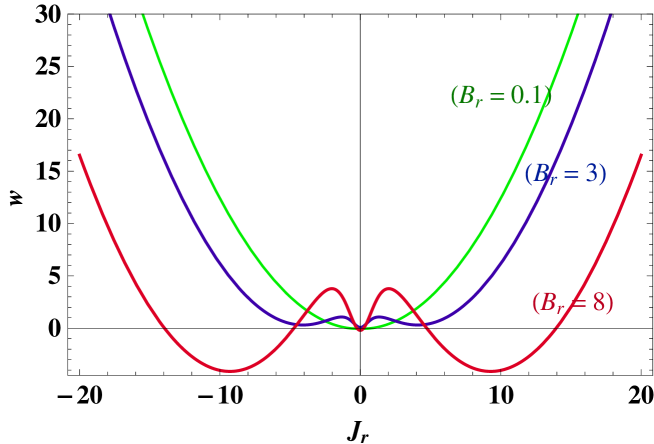
Figure 2: (Color on line). A plot of $w$ $vs$ $J_{r}$, for values of $B_{r}=0.1,\,3,\,and\,8$.

2.1 Acknowledgments

We acknowledge support from UNAM project PAPIIT-IN118610.

References

References

- [1]
- [2] M. A. Zudov, R. R. Du, J. A. Simmons, and J. L. Reno, Phys. Rev. B 64, 201311(R) (2001).
- [3] R. G. Mani, J. H. Smet, K. von Klitzing, V. Narayanamurti, W. B. Johnson, and V. Umansky, Nature 420, 646 (2002).
- [4] A. V. Andreev, I. L. Aleiner, and A. J. Millis, Phys. Rev. Lett. 91, 056803 (2003).
- [5] V. I. Ryzhii, Sov. Phys. Solid State 11, 2078 (1970).
- [6] A. C. Durst, S. Sachdev, N. Read, and S. M. Girvin, Phys. Rev. Lett. 91, 086803 (2003).
- [7] X. L. Lei and S. Y. Liu, Phys. Rev. Lett. 91, 226805 (2003).
- [8] M. G. Vavilov and I. L. Aleiner, Phys. Rev. B 69, 035303 (2004).
- [9] M. Torres and A. Kunold, Phys. Rev. B 71, 115313 (2005).
- [10] J. Inarrea and G. Platero, Phys. Rev. B 76, 073311 (2007).
- [11] I. A. Dmitriev, A. D. Mirlin, and D. G. Polyakov, Phys. Rev. Lett. 91, 226802 (2003).
- [12] I. A. Dmitriev, M. G. Vavilov, I. L. Aleiner, A. D. Mirlin, and D. G. Polyakov, Phys. Rev. B 71, 115316 (2005).
- [13] J. P. Robinson, M. P. Kennett, N. R. Cooper, and V. I. Fal’ko, Phys. Rev. Lett. 93, 036804 (2004).
- [14] A. A. Bykov, J. Q. Zhang, S. Vitkalov, A. K. Kalagin, and A. K. Bakarov, Phys. Rev. B 72, 245307 (2005).
- [15] J. Q. Zhang, S. Vitkalov, A. A. Bykov, A. K. Kalagin, and A. K. Bakarov, Phys. Rev. B 75, 081305(R) (2007).
- [16] W. Zhang, H.-S. Chiang, M. A. Zudov, L. N. Pfeiffer, and K. W. West, Phys. Rev. B 75, 041304(R) (2007).
- [17] A. A. Bykov, J. Q. Zhang, S. Vitkalov, A. K. Kalagin, and A. K. Bakarov, Phys. Rev. Lett. 99, 116801 (2007).
- [18] A. Kunold and M. Torres, Physica B 403, 3803 (2008).
- [19] A. Kunold and M. Torres, Phys. Rev. B 80, 205314 (2009).
- [20] T. Ando, A. B. Fowler, and F. Stern, Rev. Mod. Phys. 54, 437 (1982).
- [21] A. T. Hatke, M. A. Zudov, L. N. Pfeiffer, and K. W. West, Phys. Rev. B 79, 161308(R) (2009b).
- [22] A. Kunold and M. Torres, To be published.
- [23] R. K. Pathria, Statistical Mechanics (Butterworth-Heinemann, Oxford., 1996).