Robust recovery of multiple subspaces by geometric $\bolds{{l_{p}}}$ minimization

Abstract

We assume i.i.d. data sampled from a mixture distribution with $K$ components along fixed $d$-dimensional linear subspaces and an additional outlier component. For $p>0$, we study the simultaneous recovery of the $K$ fixed subspaces by minimizing the $l_{p}$-averaged distances of the sampled data points from any $K$ subspaces. Under some conditions, we show that if $0<p\leq 1$, then all underlying subspaces can be precisely recovered by $l_{p}$ minimization with overwhelming probability. On the other hand, if $K>1$ and $p>1$, then the underlying subspaces cannot be recovered or even nearly recovered by $l_{p}$ minimization. The results of this paper partially explain the successes and failures of the basic approach of $l_{p}$ energy minimization for modeling data by multiple subspaces.

T1Supported in part by NSF Grants DMS-09-15064 and DMS-09-56072.

and

1 Introduction

In the last decade, many algorithms have been developed to model data by multiple subspaces. Such hybrid linear modeling (HLM) was motivated by concrete problems in computer vision as well as by nonlinear dimensionality reduction. HLM is the simplest geometric framework for nonlinear dimensionality reduction. Nevertheless, very little theory has been developed to justify the performance of existing methods. Here we give a rigorous analysis of the recovery of multiple subspaces via an energy minimization.

One can model a data set ${\mathcal{X}}$ with $K$ subspaces obtained by minimizing the following energy over the subspaces $\mathrm{L}_{1},\ldots,\mathrm{L}_{K}$:

$$e_{l_{p}}({\mathcal{X}},\mathrm{L}_{1},\ldots,\mathrm{L}_{K})=\sum_{\mathbf{x}\in{\mathcal{X}}}\operatorname{dist}^{p}\Biggl{(}\mathbf{x},\bigcup_{i=1}^{K}\mathrm{L}_{i}\Biggr{)},$$ (1)

where $\operatorname{dist}(\cdot,\cdot)$ denotes the Euclidean distance and $p>0$ is a fixed parameter. For simplicity, we assume that $L_{1},\ldots,L_{K}$ are linear subspaces of the same dimension $d$, and we refer to them as $d$-subspaces (generalizations are discussed in Sections 5.6 and 5.7). We also assume that the data set ${\mathcal{X}}$ contains i.i.d. samples from a mixture distribution $\mu$ with $K$ components along fixed $d$-subspaces and an additional outlier component. The recovery problem asks whether with overwhelming probability the minimization of (1) recovers the underlying subspaces of $\mu$. We show here that when $p\leq 1$ the answer to this problem is positive, whereas when $p>1$ it is negative.

Recovery problems are common in statistics, for example, recovering a single subspace in least squares type problems or recovering multiple centers as in $K$-means. However, our recent setting requires novel developments. One issue is the strong geometric nature of our problem, resulting from an optimization on a product space of Grassmannians. The other is the difficulty of approximating the problem by convex optimization (as we clarify in Section 5.1). Thus, even though it is an elementary problem in statistical learning, it requires the development of techniques which are currently not widely common in statistics.

1.1 Background and related work

Many algorithms have been developed for HLM (see, e.g., Costeira98 , Torr98geometricmotion , Tipping99mixtures , Bradley00kplanes , Tseng00nearest , Kanatani01 , Ho03 , Vidal05 , Yan06LSA , Ma07 , Ma07Compression , spectralapplied , akramks08 , MKFworkshop09 , LBFjournal10 ), and they find diverse applications in several areas, such as motion segmentation in computer vision, hybrid linear representation of images, classification of face images and temporal segmentation of video sequences (see, e.g., Vidal05 , Ma07 , LBFjournal10 ). HLM is the simplest nonlinear data modeling and fits within the broader frameworks of modeling data by mixture of manifolds Arias-Castro08Surfaces and by Whitney’s stratified space stratification10 .

The $K$-subspaces algorithm Bradley00kplanes , Tseng00nearest , Ho03 is the most basic heuristic for HLM, and it suggests an iterative procedure attempting to minimize the energy (1) with $p=2$. It generalizes the $K$-means algorithm, which models data by $K$ centers, that is, $0$-dimensional affine subspaces. Numerical experiments by Zhang et al. MKFworkshop09 have shown that the $K$-subspaces algorithm is in general not robust to outliers, whereas a different method aiming to minimize (1) with $p=1$ seems to be robust to outliers.

There has been little investigation into performance guarantees of the various HLM algorithms. Nevertheless, the accuracy of segmentation under some sampling assumptions was analyzed for two spectral-type HLM algorithms in spectraltheory and Arias-Castro08Surfaces , where Arias-Castro08Surfaces also quantified the tolerance to outliers (Arias-Castro08Surfaces considers only the asymptotic case, though applies to modeling by multiple manifolds). For the $K$-means algorithm (which only applies to $0$-dimensional affine subspaces), Pollard has established strong consistency Pollard81Kmeans and a central limit theorem Pollard82KmeansCLT .

In lprecoverypart111 , we analyzed the $l_{p}$-recovery of the “most significant” subspace among multiple subspaces and outliers with spherically symmetric underlying distributions. We assume here a similar (though weaker) underlying model and rely on some of the estimates already developed there.

1.2 Basic conventions and notation

We denote by $\mathrm{G}(D,d)$ the Grassmannian, that is, the manifold of $d$-subspaces of $\mathbb{R}^{D}$. We measure distances between $\mathrm{F}$ and $\mathrm{G}$ in $\mathrm{G}(D,d)$ by the metric

$$\operatorname{dist}_{\mathrm{G}}(\mathrm{F},\mathrm{G})=\sqrt{\sum_{i=1}^{d}\theta_{i}^{2}},$$ (2)

where $\{\theta_{i}\}_{i=1}^{d}$ are the principal angles between $\mathrm{F}$ and $\mathrm{G}$. We use this distance since there is a simple formula for the geodesic lines on the Grassmannian equipped with this distance (see, e.g., lprecoverypart111 , equation 12), which is applied in this paper. We distinguish elements in the $K$-fold product space $\mathrm{G}(D,d)^{K}$ by the $l_{\infty}$ norm, that is,

$$\operatorname{dist}_{\mathrm{G}^{K}}((\mathrm{L}_{1},\ldots,\mathrm{L}_{K}),(\hat{\mathrm{L}}_{1},\ldots,\hat{\mathrm{L}}_{K}))=\max_{i=1,\ldots,K}(\operatorname{dist}_{\mathrm{G}}(\mathrm{L}_{i},\hat{\mathrm{L}}_{i})).$$ (3)

Following Mat95 , Section 3.9, we denote by $\gamma_{D,d}$ the “uniform” distribution on $\mathrm{G}(D,d)$.

We denote by $a\vee b$ and $a\wedge b$ the maximum and minimum of $a$ and $b$, respectively. We designate the support of a distribution $\mu$ by $\operatorname{supp}(\mu)$. By saying “with overwhelming probability” or, in short, “w.o.p.,” we mean that the underlying probability is at least $1-Ce^{-N/C}$, where $C$ is a constant independent of $N$.

1.3 Setting of this paper

We assume an i.i.d. data set ${\mathcal{X}}\subseteq\mathbb{R}^{D}$ of size $N$ sampled from a mixture distribution representing a hybrid linear model around distinct $d$-subspaces, $\{\mathrm{L}^{*}_{i}\}_{i=1}^{K}$. We in fact consider two different types of models, but both of them have the same basic structure.

We assume $K$ distributions, $\mu_{i}$, each supported on a corresponding and distinct $d$-subspace, $\mathrm{L}^{*}_{i}$, a noise level $\varepsilon\geq 0$, and an outlier distribution, denoted by $\mu_{0}$. Furthermore, for each $1\leq i\leq K$ we have a distinct noise distribution $\nu_{i,\varepsilon}$ with bounded support in the orthogonal complement $\mathrm{L}^{*}_{i}$. We assume that the $p$th moments of $\{\|\nu_{i,\varepsilon}\|\}_{i=1}^{K}$ are smaller than $\varepsilon^{p}$ for all $0<p\leq 1$ ($p<1$ is only needed when we consider $l_{p}$ minimization with $p<1$). Moreover, if $\varepsilon=0$, then $\{\nu_{i,0}\}_{i=1}^{K}$ are the Dirac $\delta$ distributions supported on the origin within the corresponding subspaces orthogonal to $\{\mathrm{L}^{*}_{i}\}_{i=1}^{K}$.

We assume that the underlying distributions, $\{\mu_{i}\}_{i=0}^{K}$, have bounded supports (or possibly sub-Gaussian as explained in Section 5.3). In order to simplify our estimates, we further assume that $\operatorname{supp}(\mu_{i})\subseteq{\mathrm{B}}(\mathbf{0},1)$ for $0\leq i\leq K$.

From these pieces we construct the mixture distribution $\mu_{\varepsilon}$,

$$\mu_{\varepsilon}=\alpha_{0}\mu_{0}+\sum_{i=1}^{K}\alpha_{i}\mu_{i}\times\nu_{i,\varepsilon},$$ (4)

where $\alpha_{0}\geq 0$, $\alpha_{i}>0$ $\forall 1\leq i\leq K$ and $\sum_{i=0}^{K}\alpha_{i}=1$. If $\varepsilon=0$, then for convenience we replace the notation $\mu_{\varepsilon}$ by $\mu$, that is,

$$\mu=\alpha_{0}\mu_{0}+\sum_{i=1}^{K}\alpha_{i}\mu_{i}.$$ (5)

Within this basic framework, we analyze two different models. For $\varepsilon\geq 0$ and $\mu_{\varepsilon}$ as in (4), we say that $\mu_{\varepsilon}$ is a weakly spherically symmetric HLM distribution with noise level $\varepsilon$ if the $\{\mu_{i}\}_{i=1}^{K}$ are generated by rotations (in $\mathbb{R}^{D}$) of a single distribution $\hat{\mu}$, such that $\hat{\mu}(\{\mathbf{0}\})<1$, $\operatorname{supp}(\hat{\mu})\subseteq{\mathrm{B}}(\mathbf{0},1)\cap\hat{\mathrm{L}}$ for some $d$-subspace $\hat{\mathrm{L}}\subset\mathbb{R}^{D}$ and $\hat{\mu}$ is spherically symmetric within $\hat{\mathrm{L}}$ (i.e., invariant to rotations within $\hat{\mathrm{L}}$).

Our second model has weaker assumptions on the distributions of inliers and a slightly stronger assumption on the distribution of outliers. For $\varepsilon\geq 0$ and $\mu_{\varepsilon}$ as in (4), we say that $\mu_{\varepsilon}$ is a weak HLM distribution with noise level $\varepsilon$ if $\mu_{i}(\{\mathbf{0}\})<1$ $\forall 1\leq i\leq K$, $\operatorname{supp}(\mu_{\varepsilon})\subseteq{\mathrm{B}}(\mathbf{0},1)$ and for some $r>0$ the uniform distribution on ${\mathrm{B}}(\mathbf{0},r)$ is absolutely continuous w.r.t. the restriction of $\mu_{0}$ to ${\mathrm{B}}(\mathbf{0},r)$.

Our theory uses the constant $\tau_{0}\equiv\tau_{0}(d,p,\{\mu_{i}\}_{i=1}^{K})$. We delay its definition to the proofs [see (11)], but use it in the formulation of Theorems 1.1 and 1.2.

1.4 Statistical problems of this paper

We address here two statistical problems. The simpler one is implicit in this introduction, though clear from the proofs. It asks whether the underlying subspaces $\{\mathrm{L}^{*}_{i}\}_{i=1}^{K}$ can be recovered when $\varepsilon=0$ by minimizing $\mathbb{E}_{\mu}(\operatorname{dist}^{p}(\mathbf{x},\bigcup_{i=1}^{K}\mathrm{L}_{i}))$ over $\{\mathrm{L}_{i}\}_{i=1}^{K}\subset\mathrm{G}(D,d)$. The main problem can be formulated using the empirical distribution $\mu_{N}$ of i.i.d. sample of size $N$ from $\mu$. It asks whether $\{\mathrm{L}^{*}_{i}\}_{i=1}^{K}$ can be recovered (w.o.p.) by minimizing $\mathbb{E}_{\mu_{N}}(\operatorname{dist}^{p}(\mathbf{x},\bigcup_{i=1}^{K}\mathrm{L}_{i}))$, which is equivalent to minimizing (1). In the noisy case, we extend these problems to near recovery. When $K>1$ and $d\geq 1$, these problems are nontrivial and require complicated geometric estimates.

1.5 Main theory

We first formulate the exact recovery of $\{\mathrm{L}^{*}_{i}\}_{i=1}^{K}$ as the unique global minimizer of the $l_{p}$ energy (1) when $0<p\leq 1$.

Theorem 1.1

Assume that $\mu$ is a weakly spherically symmetric HLM distribution on $\mathbb{R}^{D}$ without noise ($\varepsilon=0$) and with underlying subspaces $\{\mathrm{L}^{*}_{i}\}_{i=1}^{K}\subseteq\mathbb{R}^{D}$ and mixture coefficients $\{\alpha_{i}\}_{i=0}^{K}$. Let ${\mathcal{X}}$ be an i.i.d. data set sampled from $\mu$. If $0<p\leq 1$ and

$$\alpha_{0}<{\tau_{0}}\cdot\min_{i=1,\ldots,K}\alpha_{i}\cdot\Bigl{(}1\wedge\min_{1\leq i,j\leq K}\operatorname{dist}_{\mathrm{G}}(\mathrm{L}^{*}_{i},\mathrm{L}^{*}_{j})^{p}/2^{p}\Bigr{)},$$ (6)

then w.o.p. the set $\{\mathrm{L}^{*}_{1},\ldots,\mathrm{L}^{*}_{K}\}$ is the unique global minimizer of the energy (1) among all $d$-subspaces in $\mathbb{R}^{D}$.

Theorem 1.1 extends to the noisy case by allowing near-recovery as follows (a counterexample for asymptotic exact recovery is shown in Section 3.2).

Theorem 1.2

Assume that $\varepsilon>0$ and $\mu_{\varepsilon}$ is a weakly spherically symmetric HLM distribution of noise level $\varepsilon$ on $\mathbb{R}^{D}$ with $K$ $d$-subspaces $\{\mathrm{L}^{*}_{i}\}_{i=1}^{K}\subseteq\mathbb{R}^{D}$ and mixture coefficients $\{\alpha_{i}\}_{i=0}^{K}$. Let ${\mathcal{X}}$ be an i.i.d. data sampled from $\mu_{\varepsilon}$. If $0<p\leq 1$ and

$$\varepsilon<3^{-{1/p}}\Bigl{(}\tau_{0}\cdot\min_{i=1,\ldots,K}\alpha_{i}\cdot\Bigl{(}1\wedge\min_{1\leq i,j\leq K}\operatorname{dist}_{\mathrm{G}}(\mathrm{L}^{*}_{i},\mathrm{L}^{*}_{j})^{p}/2^{p}\Bigr{)}-\alpha_{0}\Bigr{)}^{1/p},$$ (7)

then any minimizer of (1) in $\mathrm{G}(D,d)^{K}$ has a distance smaller than

$$f\equiv f(\varepsilon,K,d,p,\{\alpha_{i}\}_{i=1}^{K})=3^{1/p}\cdot\Bigl{(}\tau_{0}\min_{1\leq j\leq K}\alpha_{j}-\alpha_{0}\Bigr{)}^{-{1/p}}\cdot\varepsilon$$ (8)

from one of the permutations of $(\mathrm{L}^{*}_{1},\ldots,\mathrm{L}^{*}_{K})$ with overwhelming probability.

At last, we formulate the impossibility to recover $\{\mathrm{L}^{*}_{i}\}_{i=1}^{K}$ by $l_{p}$ minimization when $p>1$ (the constants $\delta_{0}$ and $\kappa_{0}$ in our formulation are estimated in Section 4.5.5).

Theorem 1.3

Assume an i.i.d. sample of $K$ $d$-subspaces $\{\mathrm{L}^{*}_{i}\}_{i=1}^{K}\subset\mathrm{G}(D,d)$ from the “uniform” distribution on $\mathrm{G}(D,d)$, $\gamma_{D,d}$. For $\varepsilon\geq 0$ and the sample $\{\mathrm{L}^{*}_{i}\}_{i=1}^{K}$, let $\mu_{\varepsilon}$ be a weak HLM distribution with noise level $\varepsilon$ and let ${\mathcal{X}}$ be an i.i.d. data set of size $N$ sampled from $\mu_{\varepsilon}$. If $p>1$ and $K>1$, then for almost every $\{\mathrm{L}^{*}_{i}\}_{i=1}^{K}$ (w.r.t. $\gamma_{D,d}^{K}$) there exist positive constants $\delta_{0}$ and $\kappa_{0}$, independent of $N$, such that for any $\varepsilon<\delta_{0}$ the minimizer of (1), $\hat{\mathrm{L}}_{1},\ldots,\hat{\mathrm{L}}_{K}$, satisfies w.o.p.:

$$\operatorname{dist}_{\mathrm{G}^{K}}((\hat{\mathrm{L}}_{1},\ldots,\hat{\mathrm{L}}_{K}),(\mathrm{L}^{*}_{1},\ldots,\mathrm{L}^{*}_{K}))>\kappa_{0}.$$ (9)

The above theorems have direct implications for HLM with spherically symmetric sampling along the subspaces. Theorems 1.1 and 1.2 clarify to some extent the robustness of two recent algorithms for HLM, which use the $l_{1}$ energy (1): Median $K$-Flats (MKF) MKFworkshop09 and Local Best-fit Flats (LBF) LBFcvpr10 . Theorem 1.3 explains why common HLM strategies that use the $l_{2}$ energy (1) (e.g., $K$-subspaces) are generally not robust to outliers.

1.6 Structure of the paper

Theorems 1.1, 1.2 and 1.3 are proved in Sections 2, 3 and 4, respectively. Section 5 discusses possible extensions as well as limitations of our theory and suggests some open directions.

2 Proof of Theorem 1.1

2.1 Preliminaries

We view the energy $e_{l_{p}}({\mathcal{X}},\mathrm{L}_{1},\ldots,\mathrm{L}_{K})$ as a function defined on $\mathrm{G}(D,d)^{K}$ while being conditioned on the fixed data set ${\mathcal{X}}$. Therefore, the minimizer of $e_{l_{p}}({\mathcal{X}},\mathrm{L}_{1},\ldots,\mathrm{L}_{K})$ is an element $(\mathrm{L}^{\prime}_{1},\ldots,\mathrm{L}^{\prime}_{K})$ in $\mathrm{G}(D,d)^{K}$. Since any permutation of its $K$ coordinates in $\mathrm{G}(D,d)$ results in another minimizer, we sometimes say that the set $\{\mathrm{L}^{\prime}_{1},\ldots,\mathrm{L}^{\prime}_{K}\}$ is a minimizer [instead of $(\mathrm{L}^{\prime}_{1},\ldots,\mathrm{L}^{\prime}_{K})$].

We denote $e_{l_{p}}(\mathbf{x},\mathrm{L}_{1},\ldots,\mathrm{L}_{K}):=e_{l_{p}}(\{\mathbf{x}\},\mathrm{L}_{1},\ldots,\mathrm{L}_{K})$ and view it as a function on $\mathbb{R}^{D}\times\mathrm{G}(D,d)^{K}$.

We denote the set of all permutations of $(1,2,\ldots,K)$ by $\mathcal{P}_{K}$. We designate an open ball in $\mathrm{G}(D,d)$ by ${\mathrm{B}_{\mathrm{G}}}(\mathrm{L},r)$ as opposed to the Euclidean open ball in $\mathbb{R}^{D}$, ${\mathrm{B}}(\mathbf{x},r)$.

We partition ${\mathcal{X}}$ into the subsets $\{{\mathcal{X}}_{i}\}_{i=0}^{K}$ with $\{N_{i}\}_{i=0}^{K}$ points sampled according to the distributions $\{\mu_{i}\}_{i=0}^{K}$.

We define

$$\psi_{\mu_{1}}(t)={\mu_{1}}(\mathbf{x}\in\mathbb{R}^{D}\dvtx-t<|\mathbf{x}^{T}\mathbf{v}|<t),$$ (10)

where $\mathbf{v}$ is an arbitrarily fixed unit vector in $\mathrm{L}_{1}^{*}$ [due to the spherical symmetry of $\mu_{1}$ within $\mathrm{L}_{1}^{*}$, (10) is independent of $\mathbf{v}$]. We note that since $\{\mu_{i}\}_{i=1}^{K}$ are generated by a single distribution, $\psi_{\mu_{1}}(t)=\psi_{\mu_{i}}(t)$ $\forall 2\leq i\leq K$. The invertibility of $\psi_{\mu_{1}}$ is established in lprecoverypart111 , Appendix A.2, and an estimate of $\psi_{\mu_{1}}$ for a uniform distribution on a $d$-dimensional ball appears in lprecoverypart111 , Appendix A.1.

Theorem 1.1 uses the constant $\tau_{0}$, which we can now define as follows:

$$\tau_{0}:=\frac{(1-\mu_{1}(\{\mathbf{0}\}))\cdot 2^{p-1}\cdot\psi_{\mu_{1}}^{-1}(({1+(2K-1)\mu_{1}(\{\mathbf{0}\})})/({2K}))^{p}}{(\pi\sqrt{d})^{p}}.$$ (11)

In the special case where $\mu_{1}$ is the uniform distribution on ${\mathrm{B}}(\b{0},1)\cap\mathrm{L}_{1}$, then the estimate of $\psi_{\mu}$ in lprecoverypart111 , Section A.1, implies the following lower bound for $\tau_{0}$:

$$\tau_{0}>\frac{1}{2^{p+1}\cdot K^{p}\cdot d^{3p/2}}.$$

Consequently, Theorem 1.1 holds in this case if $\tau_{0}$ in (6) is replaced by $1/(2^{p+1}\cdot K^{p}\cdot d^{3p/2})$. Furthermore, it follows from basic scaling arguments that if $\mu_{1}$ is the uniform distribution on ${\mathrm{B}}(\b{0},r_{1})\cap\mathrm{L}_{1}$ and $\operatorname{supp}(\mu_{0})\subseteq{\mathrm{B}}(\b{0},r_{2})$, where $r_{1}$ and $r_{2}$ are any positive numbers, then

$$\tau_{0}>\frac{r_{1}^{p}}{2^{p+1}\cdot K^{p}\cdot d^{3p/2}\cdot r_{2}^{p}}.$$

2.2 Auxiliary lemmata

The following lemmata are used throughout this proof (Lemma 2.1 is proved in the Appendix and Lemma 2.2 in lprecoverypart111 , Appendix A.2).

Lemma 2.1

Suppose that $\mathrm{L}_{1},\hat{\mathrm{L}}_{1},\ldots,\hat{\mathrm{L}}_{K}\,{\in}\,\mathrm{G}(D,d),p\,{>}\,0$ and $\mu_{1}$ is a spherically symmetric distribution in ${\mathrm{B}}(\mathbf{0},1)\cap\mathrm{L}_{1}$. If $\min_{1\leq j\leq K}\operatorname{dist}_{\mathrm{G}}(\mathrm{L}_{1},\hat{\mathrm{L}}_{j})>\varepsilon$, then

$$\mathbb{E}_{{\mu}_{1}}(e_{l_{p}}(\mathbf{x},\hat{\mathrm{L}}_{1},\ldots,\hat{\mathrm{L}}_{K}))>\tau_{0}\varepsilon^{p}.$$

Lemma 2.2

For any $\mathbf{x}\in\mathbb{R}^{D}$ and $\mathrm{L}_{1},\mathrm{L}_{2}\in\mathrm{G}(D,d)$,

$$|{\operatorname{dist}}(\mathbf{x},\mathrm{L}_{1})-\operatorname{dist}(\mathbf{x},\mathrm{L}_{2})|\leq\|\mathbf{x}\|\operatorname{dist}_{\mathrm{G}}(\mathrm{L}_{1},\mathrm{L}_{2}).$$

2.3 Proof in expectation

We verify Theorem 1.1 “in expectation,” whereas later sections extend the proof to hold w.o.p. We use the following notation w.r.t. the fixed $d$-subspaces $\mathrm{L}^{*}_{1}$, $\mathrm{L}^{*}_{2},\ldots,\mathrm{L}^{*}_{K}$, $\hat{\mathrm{L}}_{1}$, $\hat{\mathrm{L}}_{2},\ldots,\hat{\mathrm{L}}_{K}\in\mathrm{G}(D,d)$:

$$I(i)=\mathop{\arg\min}_{1\leq j\leq K}\operatorname{dist}_{\mathrm{G}}(\mathrm{L}^{*}_{i},\hat{\mathrm{L}}_{j})\qquad\forall 1\leq i\leq K$$ (12)

and

$$d_{0}=\min_{i_{1},i_{2},\ldots,i_{K}\in\mathcal{P}_{K}}\operatorname{dist}_{\mathrm{G}^{K}}((\mathrm{L}^{*}_{i_{1}},\ldots,\mathrm{L}^{*}_{i_{K}}),(\hat{\mathrm{L}}_{1},\ldots,\hat{\mathrm{L}}_{K})).$$ (13)

The “expected version” of Theorem 1.1 is formulated and proved as follows.

Proposition 2.1

Suppose that $\hat{\mathrm{L}}_{1},\ldots,\hat{\mathrm{L}}_{K}$ are arbitrary subspaces in $\mathrm{G}(D,d)$, $0<p\leq 1$, and $I$ is defined w.r.t. $\{\hat{\mathrm{L}}_{i}\}_{i=1}^{K}$ and the underlying subspaces $\{\mathrm{L}^{*}_{i}\}_{i=1}^{K}$. If $(I(1),\ldots,I(K))$ is a permutation of $(1,\ldots,K)$, then

$$\mathbb{E}_{\mu}e_{{l_{p}}}(\mathbf{x},\hat{\mathrm{L}}_{1},\ldots,\hat{\mathrm{L}}_{K})-\mathbb{E}_{\mu}e_{{l_{p}}}(\mathbf{x},\mathrm{L}^{*}_{1},\ldots,\mathrm{L}^{*}_{K})$$

(14)

$$\qquad\geq\Bigl{(}\tau_{0}\min_{1\leq j\leq K}\alpha_{j}-\alpha_{0}\Bigr{)}d_{0}^{p}.$$

On the other hand, if $(I(1),\ldots,I(K))$ is not a permutation of $(1,\ldots,K)$, then

$$\mathbb{E}_{\mu}e_{{l_{p}}}(\mathbf{x},\hat{\mathrm{L}}_{1},\ldots,\hat{\mathrm{L}}_{K})-\mathbb{E}_{\mu}e_{{l_{p}}}(\mathbf{x},\mathrm{L}^{*}_{1},\ldots,\mathrm{L}^{*}_{K})$$

(15)

$$\qquad\geq\tau_{0}\Bigl{(}\min_{1\leq j\leq K}\alpha_{j}\Bigr{)}\Bigl{(}\min_{1\leq i,j\leq K}\operatorname{dist}_{\mathrm{G}}^{p}(\mathrm{L}^{*}_{i},\mathrm{L}^{*}_{j})/2\Bigr{)}-\alpha_{0}.$$

We define

$$M=\mathop{\arg\max}_{1\leq i\leq K}\operatorname{dist}_{\mathrm{G}}\bigl{(}\mathrm{L}^{*}_{i},\hat{\mathrm{L}}_{I(i)}\bigr{)}.$$

Assume first that $(I(1),\ldots,I(K))$ is a permutation of $(1,\ldots,K)$. Using the definition of $I$, we have

$$\min_{1\leq j\leq K}\operatorname{dist}_{\mathrm{G}}(\mathrm{L}^{*}_{M},\hat{\mathrm{L}}_{j}) = \operatorname{dist}_{\mathrm{G}}\bigl{(}\mathrm{L}^{*}_{M},\hat{\mathrm{L}}_{I({M})}\bigr{)}$$

$$= \operatorname{dist}_{\mathrm{G}^{K}}\bigl{(}(\mathrm{L}^{*}_{1},\ldots,\mathrm{L}^{*}_{K}),\bigl{(}\hat{\mathrm{L}}_{I(1)},\ldots,\hat{\mathrm{L}}_{I(K)}\bigr{)}\bigr{)}$$

$$= d_{0}.$$

Combining (2.3) with Lemma 2.1, we obtain that

$$\mathbb{E}_{\mu_{M}}e_{{l_{p}}}(\mathbf{x},\hat{\mathrm{L}}_{1},\ldots,\hat{\mathrm{L}}_{K})-\mathbb{E}_{\mu_{M}}e_{{l_{p}}}(\mathbf{x},\mathrm{L}^{*}_{1},\ldots,\mathrm{L}^{*}_{K})$$

(17)

$$\qquad=\mathbb{E}_{\mu_{M}}e_{{l_{p}}}(\mathbf{x},\hat{\mathrm{L}}_{1},\ldots,\hat{\mathrm{L}}_{K})>\tau_{0}d_{0}^{p}.$$

For any $\mathbf{x}\in{\mathcal{X}}_{0}$, let $m(\mathbf{x})=\arg\min_{1\leq i\leq K}\operatorname{dist}(\mathbf{x},\mathrm{L}^{*}_{i})$, $\hat{m}(\mathbf{x})=\break\arg\min_{1\leq i\leq K}\operatorname{dist}(\mathbf{x},\hat{\mathrm{L}}_{i})$ and note that

$$e_{l_{p}}(\mathbf{x},\hat{\mathrm{L}}_{1},\ldots,\hat{\mathrm{L}}_{K})-e_{l_{p}}(\mathbf{x},\mathrm{L}^{*}_{1},\ldots,\mathrm{L}^{*}_{K})$$

$$\qquad=\operatorname{dist}\bigl{(}\mathbf{x},\hat{\mathrm{L}}_{\hat{m}(\mathbf{x})}\bigr{)}^{p}-\operatorname{dist}\bigl{(}\mathbf{x},\mathrm{L}^{*}_{m(\mathbf{x})}\bigr{)}^{p}$$

$$\qquad\geq\operatorname{dist}\bigl{(}\mathbf{x},\hat{\mathrm{L}}_{\hat{m}(\mathbf{x})}\bigr{)}^{p}-\operatorname{dist}\bigl{(}\mathbf{x},\mathrm{L}^{*}_{I^{-1}(\hat{m}(\mathbf{x}))}\bigr{)}^{p}$$ (18)

$$\qquad\geq-\|\mathbf{x}\|^{p}\operatorname{dist}_{\mathrm{G}}\bigl{(}\hat{\mathrm{L}}_{\hat{m}(\mathbf{x})},\mathrm{L}^{*}_{I^{-1}(\hat{m}(\mathbf{x}))}\bigr{)}^{p}$$

$$\qquad\geq-\|\mathbf{x}\|^{p}d_{0}^{p}\geq-d_{0}^{p},$$

where the second inequality in (2.3) uses Lemma 2.2. Therefore,

$$\mathbb{E}_{\mu_{0}}e_{{l_{p}}}(\mathbf{x},\hat{\mathrm{L}}_{1},\ldots,\hat{\mathrm{L}}_{K})-\mathbb{E}_{\mu_{0}}e_{{l_{p}}}(\mathbf{x},\mathrm{L}^{*}_{1},\ldots,\mathrm{L}^{*}_{K})>-d_{0}^{p}.$$ (19)

At last, we observe that

$$\mathbb{E}_{\mu}e_{{l_{p}}}(\mathbf{x},\hat{\mathrm{L}}_{1},\ldots,\hat{\mathrm{L}}_{K})-\mathbb{E}_{\mu}e_{{l_{p}}}(\mathbf{x},\mathrm{L}^{*}_{1},\ldots,\mathrm{L}^{*}_{K})$$

$$\qquad\geq\alpha_{M}\bigl{(}\mathbb{E}_{\mu_{M}}e_{{l_{p}}}(\mathbf{x},\hat{\mathrm{L}}_{1},\ldots,\hat{\mathrm{L}}_{K})-\mathbb{E}_{\mu_{M}}e_{{l_{p}}}(\mathbf{x},\mathrm{L}^{*}_{1},\ldots,\mathrm{L}^{*}_{K})\bigr{)}$$ (20)

$$\qquad\quad{}+\alpha_{0}\bigl{(}\mathbb{E}_{\mu_{0}}e_{{l_{p}}}(\mathbf{x},\hat{\mathrm{L}}_{1},\ldots,\hat{\mathrm{L}}_{K})-\mathbb{E}_{\mu_{0}}e_{{l_{p}}}(\mathbf{x},\mathrm{L}^{*}_{1},\ldots,\mathrm{L}^{*}_{K})\bigr{)}.$$

The proposition in this case thus follows from (2.3), (19) and (2.3).

Next, we assume that $I(1),\ldots,I(K)$ is not a permutation of $1,2,\ldots,K$. In this case, there exist $1\leq n_{1},n_{2}\leq K$ such that $I(n_{1})=I(n_{2})$ and, consequently,

$$2\min_{1\leq j\leq K}\operatorname{dist}_{\mathrm{G}}(\mathrm{L}^{*}_{M},\hat{\mathrm{L}}_{j}) = 2\operatorname{dist}_{\mathrm{G}}\bigl{(}\mathrm{L}^{*}_{M},\hat{\mathrm{L}}_{I({M})}\bigr{)}$$

$$\geq \operatorname{dist}_{\mathrm{G}}\bigl{(}\mathrm{L}^{*}_{n_{1}},\hat{\mathrm{L}}_{I(n_{1})}\bigr{)}+\operatorname{dist}_{\mathrm{G}}\bigl{(}\mathrm{L}^{*}_{n_{2}},\hat{\mathrm{L}}_{I(n_{2})}\bigr{)}$$

$$\geq \operatorname{dist}_{\mathrm{G}}(\mathrm{L}^{*}_{n_{1}},\mathrm{L}^{*}_{n_{2}})$$

$$\geq \min_{1\leq i,j\leq K}\operatorname{dist}_{\mathrm{G}}(\mathrm{L}^{*}_{i},\mathrm{L}^{*}_{j}).$$

Combining (2.3) and Lemma 2.1 [applied with $\varepsilon=\min_{1\leq i,j\leq K}\operatorname{dist}_{\mathrm{G}}(\mathrm{L}^{*}_{i},\break\mathrm{L}^{*}_{j})/2$], we obtain that

$$\mathbb{E}_{\mu_{M}}e_{{l_{p}}}(\mathbf{x},\hat{\mathrm{L}}_{1},\ldots,\hat{\mathrm{L}}_{K})-\mathbb{E}_{\mu_{M}}e_{{l_{p}}}(\mathbf{x},\mathrm{L}^{*}_{1},\ldots,\mathrm{L}^{*}_{K})$$

(22)

$$\qquad>\tau_{0}\Bigl{(}\min_{1\leq i,j\leq K}\operatorname{dist}_{\mathrm{G}}(\mathrm{L}^{*}_{i},\mathrm{L}^{*}_{j})/2\Bigr{)}^{p}.$$

Finally, since the support of $\mu_{0}$ is contained in ${\mathrm{B}}(\mathbf{0},1)$, we note that

$$\mathbb{E}_{\mu_{0}}e_{{l_{p}}}(\mathbf{x},\hat{\mathrm{L}}_{1},\ldots,\hat{\mathrm{L}}_{K})-\mathbb{E}_{\mu_{0}}e_{{l_{p}}}(\mathbf{x},\mathrm{L}^{*}_{1},\ldots,\mathrm{L}^{*}_{K})\geq-1.$$ (23)

The proposition is thus concluded from (2.3), (2.3) and (23).

2.4 Proof in a local ball by calculus on the Grassmannian

We cannot directly extend (2.1) to an estimate w.o.p., since its lower bound is a multiplication of $d_{0}^{p}$, which approaches zero as the set $\{\mathrm{L}_{i}\}_{i=1}^{K}$ approaches $\{\mathrm{L}^{*}_{i}\}_{i=1}^{K}$. We will need to exclude a ball in $\mathrm{G}(D,d)^{K}$ around $\{\mathrm{L}^{*}_{i}\}_{i=1}^{K}$ before such an extension. We thus prove here that $\{\mathrm{L}^{*}_{i}\}_{i=1}^{K}$ is a unique global minimizer w.o.p. in a local ball. In Section 2.5 we extend Proposition 2.1 to an estimate w.o.p. outside this ball and conclude the theorem.

We show that there exists a sufficiently small number $\gamma_{1}$ such that $\{\mathrm{L}^{*}_{i}\}_{i=1}^{K}$ is the unique global minimizer w.o.p. of $e_{l_{p}}$ in ${\mathrm{B}_{\mathrm{G}}}((\mathrm{L}^{*}_{i_{1}},\ldots,\mathrm{L}^{*}_{i_{K}}),\gamma_{1})$. Since $e_{l_{p}}$ is permutation invariant, it is also the unique global minimizer in

$$\bigcup_{i_{1},i_{2},\ldots,i_{K}\in\mathcal{P}_{K}}{\mathrm{B}_{\mathrm{G}}}((\mathrm{L}^{*}_{i_{1}},\ldots,\mathrm{L}^{*}_{i_{K}}),\gamma_{1}).$$

In order to simplify notation in this part of the proof, we will adopt WLOG the convention that the RHS of (3) occurs at $i=1$, that is,

$$\operatorname{dist}_{\mathrm{G}}(\mathrm{L}^{*}_{1},\hat{\mathrm{L}}_{1})=\max_{i=1,\ldots,K}(\operatorname{dist}_{\mathrm{G}}(\mathrm{L}^{*}_{i},\hat{\mathrm{L}}_{i})).$$ (24)

Following this convention and the fact that $e_{l_{p}}(\sum_{i=2}^{K}{\mathcal{X}}_{i},\mathrm{L}^{*}_{1},\ldots,\mathrm{L}^{*}_{K})=0$, it is enough to prove that $(\mathrm{L}^{*}_{1},\ldots,\mathrm{L}^{*}_{K})$ is the unique global minimizer w.o.p. of $e_{l_{p}}({\mathcal{X}}_{0}\cup{\mathcal{X}}_{1},\mathrm{L}_{1},\ldots,\mathrm{L}_{K})$ in ${\mathrm{B}_{\mathrm{G}}}((\mathrm{L}^{*}_{1},\ldots,\mathrm{L}^{*}_{K}),\gamma_{1})$, for sufficiently small $\gamma_{1}$.

Let $t_{0}:=\operatorname{dist}_{\mathrm{G}}(\mathrm{L}^{*}_{1},\hat{\mathrm{L}}_{1})$. For each $1\leq i\leq K$, we parametrize according to arc length the geodesic lines from $\mathrm{L}^{*}_{i}$ to $\hat{\mathrm{L}}_{i}$ by functions $\mathrm{L}_{i}(t)$, $1\leq i\leq K$, on the interval $[0,t_{0}]$ such that

$$\mathrm{L}_{i}(0)=\mathrm{L}^{*}_{i}\quad\mbox{and}\quad\mathrm{L}_{i}(t_{0})=\hat{\mathrm{L}}_{i}.$$ (25)

We will prove that for sufficiently small $\gamma_{1}>0$,

$$\quad\frac{{\mathrm{d}}}{{\mathrm{d}}t^{p}}\bigl{(}e_{l_{p}}\bigl{(}{\mathcal{X}}_{0}\cup{\mathcal{X}}_{1},\mathrm{L}_{1}(t),\ldots,\mathrm{L}_{K}(t)\bigr{)}\bigr{)}>0\qquad\mbox{for all $0\leq t\leq\gamma_{1}$ w.o.p.}$$ (26)

This will clearly imply our desired result.

Our proof of (26) is based on the following estimate:

$$\frac{{\mathrm{d}}}{{\mathrm{d}}t^{p}}(e_{l_{p}}(\mathbf{x},\mathrm{L}_{1}(t),\ldots,\mathrm{L}_{K}(t)))\bigg{|}_{t=0}\geq-\|\mathbf{x}\|.$$ (27)

In order to establish (27), we denote $j=\arg\min_{1\leq i\leq K}\operatorname{dist}(\mathbf{x},\mathrm{L}^{*}_{i})$ and apply Lemma 2.2 to obtain that

$$\qquad\frac{{\mathrm{d}}}{{\mathrm{d}}t^{p}}(e_{l_{p}}(\mathbf{x},\mathrm{L}_{1}(t),\ldots,\mathrm{L}_{K}(t)))\bigg{|}_{t=0} = \lim_{t\rightarrow 0}\frac{\operatorname{dist}(\mathbf{x},\mathrm{L}_{j}(t))^{p}-\operatorname{dist}(\mathbf{x},\mathrm{L}_{j}(0))^{p}}{t^{p}}$$

$$\geq -\|\mathbf{x}\|\lim_{t\rightarrow 0}\frac{\operatorname{dist}_{\mathrm{G}}(\mathrm{L}_{j}(t),\mathrm{L}_{j}(0))^{p}}{t^{p}}.$$

We also note that for all $0\leq t\leq t_{0}$,

$$\frac{\operatorname{dist}_{\mathrm{G}}(\mathrm{L}_{j}(t),\mathrm{L}_{j}(0))^{p}}{t^{p}}\leq\frac{\operatorname{dist}_{\mathrm{G}}(\mathrm{L}_{1}(t),\mathrm{L}_{1}(0))^{p}}{t^{p}}=1.$$ (29)

Indeed, if $t=t_{0}$, the inequality in (29) follows from (24) and the equality follows from (25). Moreover, both of them extend to $0\leq t<t_{0}$ by the underlying property of arc length parametrization. Equation (27) thus follows from (2.4) and (29).

Combining (27) with Hoeffding’s inequality, we obtain that

$$\quad\frac{{\mathrm{d}}}{{\mathrm{d}}t^{p}}(e_{l_{p}}({\mathcal{X}}_{0},\mathrm{L}_{1}(t),\ldots,\mathrm{L}_{K}(t)))\bigg{|}_{t=0}\geq-\sum_{\mathbf{x}\in{\mathcal{X}}_{0}}\|\mathbf{x}\|\geq-\alpha_{0}N\qquad\mbox{w.o.p.}$$ (30)

We similarly derive an equation analogous to (30) when replacing ${\mathcal{X}}_{0}$ with ${\mathcal{X}}_{1}$ by applying some arguments of the proof of Lemma 2.1 and Hoeffding’s inequality as follows:

$$\frac{{\mathrm{d}}}{{\mathrm{d}}t^{p}}(e_{l_{p}}({\mathcal{X}}_{1},\mathrm{L}_{1}(t),\ldots,\mathrm{L}_{K}(t)))\bigg{|}_{t=0} = \frac{{\mathrm{d}}}{{\mathrm{d}}t}(e_{l_{1}}({\mathcal{X}}_{1},\mathrm{L}_{1}(t)))\bigg{|}_{t=0}$$

$$\geq \tau_{0}\alpha_{1}N\qquad\mbox{w.o.p.}$$

At last, combining (30), (2.4) and (6), we obtain that there exists $\gamma_{1}^{\prime}\equiv\gamma_{1}^{\prime}(D,d,K,p,\alpha_{0},\alpha_{1})$ such that w.o.p.

$$\frac{{\mathrm{d}}}{{\mathrm{d}}t^{p}}\bigl{(}e_{l_{p}}\bigl{(}{\mathcal{X}}_{0}\cup{\mathcal{X}}_{1},\mathrm{L}_{1}(t),\ldots,\mathrm{L}_{K}(t)\bigr{)}\bigr{)}\bigg{|}_{t=0}\geq(\tau_{0}\alpha_{1}-\alpha_{0})N>\gamma_{1}^{\prime}N.$$

Using the arguments of the proof of lprecoverypart111 , equation (35), we conclude that there exists a constant $\gamma_{1}\equiv\gamma_{1}(D,d,K,p,\alpha_{0},\alpha_{1},\min_{2\leq i\leq K}\operatorname{dist}(\mathrm{L}_{1}^{*},\mathrm{L}_{i}^{*}),\break\mu_{0},\mu_{1})>0$ such that (26) holds.

2.5 Conclusion of Theorem 1.1

In order to conclude the theorem, it is enough to prove that $\{\mathrm{L}^{*}_{1},\ldots,\mathrm{L}^{*}_{K}\}$ is the unique global minimizer w.o.p. of $e_{l_{p}}({\mathcal{X}}_{0}\cup{\mathcal{X}}_{1},\mathrm{L}_{1},\ldots,\mathrm{L}_{K})$ in the set

$$\mathrm{GP}(D,d,\gamma_{1}):=\mathrm{G}(D,d)^{K}\Bigm{\backslash}\bigcup_{i_{1},i_{2},\ldots,i_{K}\in\mathcal{P}_{K}}{\mathrm{B}_{\mathrm{G}}}((\mathrm{L}^{*}_{i_{1}},\ldots,\mathrm{L}^{*}_{i_{K}}),\gamma_{1}).$$ (32)

Combining Proposition 2.1, the fact that $d_{0}>\gamma_{1}$ [which follows from the definition of $d_{0}$ in (13)], Hoeffding’s inequality and (6), we obtain that there exists $\gamma_{2}\equiv\gamma_{2}(D,d,K,p,\alpha_{0},\min_{1\leq i\leq K}\alpha_{i},\min_{1\leq i\neq j\leq K}\operatorname{dist}(\mathrm{L}_{i}^{*},\mathrm{L}_{j}^{*}),\mu_{0},\mu_{1})>0$ such that for any fixed $(\hat{\mathrm{L}}_{1},\ldots,\hat{\mathrm{L}}_{K})\in\mathrm{GP}(D,d,\gamma_{1})$,

$$e_{l_{p}}({\mathcal{X}},\hat{\mathrm{L}}_{1},\ldots,\hat{\mathrm{L}}_{K})-e_{l_{p}}({\mathcal{X}},\mathrm{L}^{*}_{1},\ldots,\mathrm{L}^{*}_{K})>\gamma_{2}N\qquad\mbox{w.o.p.}$$ (33)

Following the proof of lprecoverypart111 , Theorem 1.1 [i.e., covering $\mathrm{GP}(D,d,\gamma_{1})$ by balls], we easily extend (33) w.o.p. for all $K$ subspaces in the set $\mathrm{GP}(D,d,\gamma_{1})$ (instead of fixed ones) and thus conclude the theorem.

3 Proof of Theorem 1.2 and a counterexample to asymptotic recovery

3.1 Proof of Theorem 1.2

Following the argument of lprecoverypart111 , Section 3.5.1, we reduce the verification of Theorem 1.2 to proving that there exists a constant $\gamma_{3}>0$ such that if for all permutations $i_{1},\ldots,i_{K}\in\mathcal{P}_{K}$, $\hat{\mathrm{L}}_{1},\ldots,\hat{\mathrm{L}}_{K}\in\mathrm{G}(D,d)$ satisfy that $\operatorname{dist}_{\mathrm{G}^{K}}((\mathrm{L}^{*}_{i_{1}},\ldots,\mathrm{L}^{*}_{i_{K}})$, $(\hat{\mathrm{L}}_{1},\ldots,\hat{\mathrm{L}}_{K}))>f$, then

$$\mathbb{E}_{\mu}(e_{l_{p}}(\mathbf{x},\hat{\mathrm{L}}_{1},\ldots,\hat{\mathrm{L}}_{K}))>\mathbb{E}_{\mu}(e_{l_{p}}(\mathbf{x},\mathrm{L}^{*}_{1},\ldots,\mathrm{L}^{*}_{K}))+\gamma_{3}+2\varepsilon^{p}.$$ (34)

In view of Proposition 2.1, in order to conclude (34), it is sufficient to verify that

$$\Bigl{(}\tau_{0}\min_{1\leq j\leq K}\alpha_{j}-\alpha_{0}\Bigr{)}f^{p}>\gamma_{3}+2\varepsilon^{p}$$ (35)

and

$$\tau_{0}\min_{1\leq j\leq K}\alpha_{j}\min_{1\leq i,j\leq K}\operatorname{dist}_{\mathrm{G}}^{p}(\mathrm{L}^{*}_{i},\mathrm{L}^{*}_{j})/2^{p}-\alpha_{0}>\gamma_{3}+2\varepsilon^{p}.$$ (36)

Setting $\gamma_{3}=\varepsilon^{p}/2$, (35) follows from (8) and (36) follows from (7).

3.1.1 Remark on the size of $\varepsilon$

If

$$\varepsilon>\pi\sqrt{d}3^{-{1/p}}\Bigl{(}\tau_{0}\min_{1\leq j\leq K}\alpha_{j}-\alpha_{0}\Bigr{)}^{1/p}/2,$$ (37)

then $f>\pi\sqrt{d}/2$, so that there is no restriction on the minimizer of (1) in $\mathrm{G}(D,d)^{K}$. It thus makes sense to further restrict $\varepsilon$ to be at least lower than the right-hand side of (37).

3.2 A counterexample to exact asymptotic recovery with noise

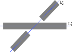
One may ask if it is possible in the noisy setting ($\varepsilon>0$) to recover the underlying subspaces as the number of sampled points, $N$, approaches infinity. The answer to this question is positive when $K=1$ (see, e.g., Anderson84 , Section 11.6, Shawe-taylor05 ) or $d=0$ (see Pollard82KmeansCLT ). However, it is often negative when $d>1$ and $K>1$, as we demonstrate in Figure 1(a) and

(a)	(b)

Figure 1: A counterexample showing that exact recovery with noise is impossible even asymptotically. (a) Gray regions of uniform distributions around the two underlying lines. (b) The gray region is the intersection of ${\mathrm{Y}}_{1}$ with the uniform distribution region around $\mathrm{L}^{*}_{1}$. The best $l_{p}$ line in ${\mathrm{Y}}_{1}$ is $\tilde{\mathrm{L}}_{1}$.

explain below. In this example, $D=2$, $K=2$, $d=1$, $\alpha_{0}=0$ and the two underlying distributions $\mu_{1}$ and $\mu_{2}$ (corresponding to the two underlying lines $\mathrm{L}^{*}_{1}$ and $\mathrm{L}^{*}_{2}$) are uniformly distributed in the two gray regions demonstrated in this figure (the region around $\mathrm{L}_{1}^{*}$ is a rectangle and the region around $\mathrm{L}_{2}^{*}$ is a union of two disjoint rectangles).

In order to verify that this is indeed a counterexample, we use a Voronoi-type region, which allows us to reduce approximation by multiple subspaces to approximation by a single subspace on it. Such regions $\{{\mathrm{Y}}_{i}\}_{i=1}^{K}$, which are frequently used in Section 4, are obtained by a Voronoi diagram (restricted to the unit ball) of given $d$-subspaces $\{\mathrm{L}_{i}\}_{i=1}^{K}\subseteq\mathrm{G}(D,d)$ as follows:

$${\mathrm{Y}}_{i}(\mathrm{L}_{1},\ldots,\mathrm{L}_{K})$$

(38)

$$\qquad=\{\mathbf{x}\in{\mathrm{B}}(\mathbf{0},1)\dvtx\operatorname{dist}(\mathbf{x},\mathrm{L}_{i})<\operatorname{dist}(\mathbf{x},\mathrm{L}_{j})\mbox{ }\forall j\dvtx 1\leq j\neq i\leq K\}.$$

These regions are useful to us due to the following elementary proposition, whose trivial proof is described in the Appendix.

Proposition 3.1

If ${\mathrm{L}}^{\prime}_{1},\ldots,{\mathrm{L}}^{\prime}_{K}\in\mathrm{G}(D,d)$, $\nu$ is a probability measure on $\mathbb{R}^{D}$ and

$$({\mathrm{L}}^{\prime}_{1},\ldots,{\mathrm{L}}^{\prime}_{K})=\mathop{\arg\min}_{({\mathrm{L}}_{1},\ldots,{\mathrm{L}}_{K})\in\mathrm{G}(D,d)^{K}}\mathbb{E}_{\nu}(e_{l_{p}}(\mathbf{x},{\mathrm{L}}_{1},\ldots,{\mathrm{L}}_{K})),$$

then

$$\mathrm{L}^{\prime}_{1}=\mathop{\arg\min}_{\mathrm{L}_{1}\in\mathrm{G}(D,d)}\mathbb{E}_{\nu}\bigl{(}e_{l_{p}}(\mathbf{x},\mathrm{L}_{1})I\bigl{(}\mathbf{x}\in{\mathrm{Y}}_{1}({\mathrm{L}}^{\prime}_{1},{\mathrm{L}}^{\prime}_{2},\ldots,{\mathrm{L}}^{\prime}_{K})\bigr{)}\bigr{)}.$$ (39)

We claim that for any fixed $p>0$, the distance between $\{\mathrm{L}^{*}_{1},\mathrm{L}^{*}_{2}\}$ and the global minimizer of (1) in the setting of this example is bounded from below w.o.p. by a positive constant independent of the sample size, $N$, for sufficiently large $N$. Equivalently, we claim that the distance between $\{\mathrm{L}^{*}_{1},\mathrm{L}^{*}_{2}\}$ and the global minimizer of $\mathbb{E}_{\mu_{\varepsilon}}(\operatorname{dist}^{p}(\mathbf{x},\bigcup_{i=1}^{K}\mathrm{L}_{i}))$ is positive, where $\mu_{\varepsilon}$ is the underlying mixture distribution for this example. In view of Proposition 3.1, we only need to show a positive distance between $\mathrm{L}^{*}_{1}$ and the minimizer of $\mathbb{E}_{\mu_{\varepsilon}}(e_{l_{p}}(\mathbf{x},\mathrm{L})I(\mathbf{x}\in{\mathrm{Y}}_{1}))$, where ${\mathrm{Y}}_{1}={\mathrm{Y}}_{1}(\mathrm{L}_{1}^{*},\mathrm{L}_{2}^{*})$. We refer to this minimizer as the best $l_{p}$ line for ${\mathrm{Y}}_{1}$ and denote it by $\tilde{\mathrm{L}}_{1}$ (while arbitrarily fixing $p$). We note that for any $p>0$, the integral of $l_{p}$ distances of points in the part of ${\mathrm{Y}}_{1}$ above $\mathrm{L}_{1}^{*}$ from the line $\mathrm{L}_{1}^{*}$ is smaller than the similar integral in the bottom part. Therefore, $\tilde{\mathrm{L}}_{1}$ is different than $\mathrm{L}^{*}_{1}$ and the respective orientation of the two lines is demonstrated in Figure 1(b). The claim is thus concluded.

4 Proof of Theorem 1.3

4.1 Preliminaries

4.1.1 Notation

We designate the projection from $\mathbb{R}^{D}$ onto its subspace $\mathrm{L}$ by $P_{\mathrm{L}}$ and the corresponding orthogonal projection by $P^{\perp}_{\mathrm{L}}$. We define

$$\mathbf{D}_{\mathrm{L},\mathbf{x},p}=P_{\mathrm{L}}(\mathbf{x})P^{\perp}_{\mathrm{L}}(\mathbf{x})^{T}\operatorname{dist}(\mathbf{x},\mathrm{L})^{(p-2)}.$$ (40)

We frequently use the Voronoi-type regions $\{{\mathrm{Y}}_{i}\}_{i=1}^{K}$ defined in (3.2) with respect to the subspaces $\{\mathrm{L}^{*}_{i}\}_{i=1}^{K}$ and possibly two additional arbitrary subspaces denoted by $\hat{\mathrm{L}}_{2}\in\mathrm{G}(D,d)$ and $\tilde{\mathrm{L}}_{2}\in\mathrm{G}(D,d)$. We will use the following short notation for $1\leq i\leq K$:

$$\hat{{\mathrm{Y}}}_{i}={\mathrm{Y}}_{i}(\mathrm{L}^{*}_{1},\hat{\mathrm{L}}_{2},\mathrm{L}^{*}_{3},\ldots,\mathrm{L}^{*}_{K}),\qquad\tilde{{\mathrm{Y}}}_{i}={\mathrm{Y}}_{i}(\mathrm{L}^{*}_{1},\tilde{\mathrm{L}}_{2},\mathrm{L}^{*}_{3},\ldots,\mathrm{L}^{*}_{K})$$ (41)

and

$${{\mathrm{Y}}}_{i}={\mathrm{Y}}_{i}(\mathrm{L}^{*}_{1},\mathrm{L}^{*}_{2},\mathrm{L}^{*}_{3},\ldots,\mathrm{L}^{*}_{K}).$$ (42)

We denote by $\bar{{\mathrm{Y}}}_{i}$ the closure of ${\mathrm{Y}}_{i}$, that is,

$$\bar{{\mathrm{Y}}}_{i}=\{\mathbf{x}\in{\mathrm{B}}(\mathbf{0},1)\dvtx\operatorname{dist}(\mathbf{x},\mathrm{L}^{*}_{i})\leq\operatorname{dist}(\mathbf{x},\mathrm{L}^{*}_{j})\mbox{ }\forall j\dvtx 1\leq j\neq i\leq K\}.$$ (43)

Similarly, the closure of $\hat{{\mathrm{Y}}}_{i}$ is denoted by $\bar{\hat{{\mathrm{Y}}}}_{i}$.

Let $\mathcal{L}_{k}$ denote the $k$th-dimensional Lebesgue measure. We denote $d^{*}=d\wedge(D-d)$ and let $\theta_{d^{*}}(\mathrm{L}^{*}_{i},\mathrm{L}^{*}_{j})$ be the $d^{*}$th largest principal angle between the $d$-subspaces $\mathrm{L}^{*}_{i}$ and $\mathrm{L}^{*}_{j}$. Our analysis uses the distribution $\mu\equiv\alpha_{0}\mu_{0}+\sum_{i=1}^{K}\alpha_{i}\mu_{i}$, even though the underlying distribution of our model is $\mu_{\varepsilon}$. For $\mathrm{L}$, $\mathrm{L}^{*}\in\mathrm{G}(D,d)$, we define the “orthogonal subtraction” $\ominus$ as follows:

$${\mathrm{L}^{*}}\ominus{\mathrm{L}}=\mathrm{L}^{*}\cap(\mathrm{L}\cap\mathrm{L}^{*})^{\perp}.$$

4.1.2 Auxiliary lemmata

Using the notation above, we formulate two lemmata, which will be used throughout this proof. The proof of Lemma 4.1 is identical to that of lprecoverypart111 , Proposition 2.2 (while replacing sums by expectations), whereas Lemma 4.2 is proved in the Appendix.

Lemma 4.1

For any $\mathrm{L}^{*}\in\mathrm{G}(D,d)$ and distribution $\mu$, a necessary condition for $\mathrm{L}^{*}$ to be a local minimum of $\mathbb{E}_{\mu}(l_{p}(\mathbf{x},\mathrm{L}))$ is

$$\mathbb{E}_{\mu}(\mathbf{D}_{\mathrm{L}^{*},\mathbf{x},p})=\mathbf{0}.$$ (44)

The next lemma quantifies the sensitivity of the region ${\mathrm{Y}}_{j}$, where $1\leq j\leq K$, to perturbations in the subspace $\mathrm{L}_{i}$, where $1\leq i\neq j\leq K$. WLOG we formulate it with $j=1$ and $i=2$ [note that we use the short notation of (41)].

Lemma 4.2

If $\hat{\mathrm{L}}_{2},\mathrm{L}^{*}_{1},\mathrm{L}^{*}_{2},\ldots,\mathrm{L}^{*}_{K}$ are subspaces in $\mathrm{G}(D,d)$ such that $\hat{\mathrm{L}}_{2}\neq\mathrm{L}^{*}_{2}$,

$$\min_{j\neq 2}(\theta_{d^{*}}(\hat{\mathrm{L}}_{2},\mathrm{L}^{*}_{j}))>0,\qquad\min_{1\leq i\neq j\leq K}(\theta_{d^{*}}(\mathrm{L}^{*}_{i},\mathrm{L}^{*}_{j}))>0$$ (45)

and

$$\theta_{d^{*}}(\hat{\mathrm{L}}_{2},\mathrm{L}^{*}_{1})\vee\theta_{d^{*}}(\mathrm{L}^{*}_{2},\mathrm{L}^{*}_{1})\leq\min_{3\leq i\leq K}\theta_{d^{*}}(\mathrm{L}^{*}_{i},\mathrm{L}^{*}_{1}),$$ (46)

then

$$\mathcal{L}_{D}\bigl{(}(\hat{{\mathrm{Y}}}_{1}\setminus{\mathrm{Y}}_{1})\cup({{\mathrm{Y}}}_{1}\setminus\hat{{\mathrm{Y}}}_{1})\bigr{)}>0.$$ (47)

4.2 A special case

The proof of Theorem 1.3 is rather involved. In order to develop a simple intuition, we provide an elementary proof of the very special case where $d=1$, $p=2$ and $K=2$. For simplicity we also assume that $D=2$, though our argument easily extends to $D>2$. Figure 2 shows the two underlying

Figure 2: Illustrative proof of Theorem 1.3 in the special case where $p=2$, $d=1$, $D=2$ and $K=2$.

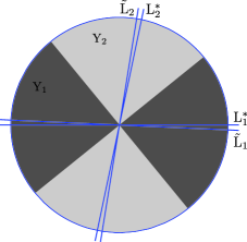
lines $\mathrm{L}^{*}_{1}$ and $\mathrm{L}^{*}_{2}$ and their corresponding regions ${\mathrm{Y}}_{1}$ and ${\mathrm{Y}}_{2}$. We note that the best $l_{2}$ lines [in $\mathrm{G}(D,1)$] for $\mu_{0}$ restricted to ${\mathrm{Y}}_{1}$ and ${\mathrm{Y}}_{2}$ are the central axes of those regions. Since $\alpha_{0}>0$, the best $l_{2}$ lines [in $\mathrm{G}(D,1)$] for $\mu$ restricted to ${\mathrm{Y}}_{1}$ and ${\mathrm{Y}}_{2}$ (denoted by $\tilde{\mathrm{L}}_{1}$ and $\tilde{\mathrm{L}}_{2}$, resp.) must reside between the best $l_{2}$ lines for $\mu_{0}$ restricted to ${\mathrm{Y}}_{1}$ and ${\mathrm{Y}}_{2}$ and $\mathrm{L}^{*}_{1}$ and $\mathrm{L}^{*}_{2}$, respectively. In particular, they are different from $\mathrm{L}^{*}_{1}$ and $\mathrm{L}^{*}_{2}$ as demonstrated in the figure. Therefore, $\mathbb{E}_{{\mu}}(e_{l_{2}}(\mathbf{x},\mathrm{L}^{*}_{1},\mathrm{L}^{*}_{2}))>\mathbb{E}_{{\mu}}(e_{l_{2}}(\mathbf{x},\tilde{\mathrm{L}}_{1},\tilde{\mathrm{L}}_{2}))$. This implies that w.o.p. $e_{l_{2}}({\mathcal{X}},\mathrm{L}^{*}_{1},\mathrm{L}^{*}_{2})>e_{l_{2}}({\mathcal{X}},\tilde{\mathrm{L}}_{1},\tilde{\mathrm{L}}_{2})$.

4.3 Reduction of the statement of Theorem 1.3 to simpler formulations

4.3.1 Reduction I: Using the Voronoi-type regions $\{{\mathrm{Y}}_{i}\}_{i=1}^{K}$

We will show here that the following equation implies Theorem 1.3:

$$\qquad\gamma_{D,d}^{K}\bigl{(}\{\mathrm{L}^{*}_{i}\}_{i=1}^{K}\subset\mathrm{G}(D,d)\dvtx\mathbb{E}_{\mu_{0}}\bigl{(}I(\mathbf{x}\in{\mathrm{Y}}_{j})\mathbf{D}_{\mathrm{L}^{*}_{j},\mathbf{x},p}\bigr{)}=\mathbf{0}\ \forall 1\leq j\leq K\bigr{)}=0.$$ (48)

First, we apply the argument of lprecoverypart111 , Section 3.6.1 (which requires the assumption specified in Section 1.3 that the first moments of $\{\|\nu_{i,\varepsilon}\|\}_{i=1}^{K}$ are smaller than $\varepsilon$) to obtain that Theorem 1.3 follows by the equation

$$\gamma_{D,d}^{K}\Bigl{(}\{\mathrm{L}^{*}_{i}\}_{i=1}^{K}\subset\mathrm{G}(D,d)\dvtx(\mathrm{L}^{*}_{1},\ldots,\mathrm{L}^{*}_{K})$$

(49)

$$\hphantom{\gamma_{D,d}^{K}\Bigl{(}}=\mathop{\arg\min}_{({\mathrm{L}}_{1},\ldots,{\mathrm{L}}_{K})}\mathbb{E}_{\mu}(e_{l_{p}}(\mathbf{x},{\mathrm{L}}_{1},\ldots,{\mathrm{L}}_{K}))\Bigr{)}=0.$$

Next, applying Proposition 3.1, we conclude that (4.3.1) is a direct consequence of the equation:

$$\gamma_{D,d}^{K}\Bigl{(}\{\mathrm{L}^{*}_{i}\}_{i=1}^{K}\subset\mathrm{G}(D,d)\dvtx\mathrm{L}^{*}_{j}=\mathop{\arg\min}_{\mathrm{L}\in\mathrm{G}(D,d)}\mathbb{E}_{\mu}\bigl{(}e_{l_{p}}(\mathbf{x},\mathrm{L})I(\mathbf{x}\in{\mathrm{Y}}_{j})\bigr{)}$$

(50)

$$\qquad\hskip 210.3pt\forall 1\leq j\leq K\Bigr{)}=0.$$

Furthermore, applying Lemma 4.1 with $\mu=\mu|_{{\mathrm{Y}}_{j}}$, we obtain that (4.3.1) follows by the equation

$$\qquad\gamma_{D,d}^{K}\bigl{(}\{\mathrm{L}^{*}_{i}\}_{i=1}^{K}\subset\mathrm{G}(D,d)\dvtx\mathbb{E}_{\mu}\bigl{(}I(\mathbf{x}\in{\mathrm{Y}}_{j})\mathbf{D}_{\mathrm{L}^{*}_{j},\mathbf{x},p}\bigr{)}=0\mbox{ }\forall 1\leq j\leq K\bigr{)}=0.$$ (51)

At last we conclude the desired reduction by noting that (51) and (48) are equivalent [indeed, the only relevant components of the distribution $\mu$ in (51) are $\mu_{0}$ and $\mu_{j}$ and the corresponding expectation according to $\mu_{j}$ is zero].

4.3.2 Reduction II: From $K$ subspaces to a single subspace

We reduce (48) so that its underlying condition involves a single subspace as follows:

$$\gamma_{D,d}\Bigl{(}\mathrm{L}^{*}_{2}\in\mathrm{G}(D,d)\dvtx\min_{1\leq i\neq j\leq K}\theta_{d^{*}}(\mathrm{L}^{*}_{i},\mathrm{L}^{*}_{j})>0,$$

(52)

$$\hphantom{\gamma_{D,d}\Bigl{(}}\mathop{\arg\min}_{2\leq i\leq K}\theta_{d^{*}}(\mathrm{L}^{*}_{1},\mathrm{L}^{*}_{i})=2,\mathbb{E}_{\mu_{0}}\bigl{(}I(\mathbf{x}\in{\mathrm{Y}}_{1})\mathbf{D}_{\mathrm{L}^{*}_{1},\mathbf{x},p}\bigr{)}=\mathbf{0}\Bigr{)}=0.$$

We remark that some of the underlying technical conditions of (4.3.2) appear in (45) and (46) and will be better understood later when applying Lemma 4.2.

We verify this reduction as follows. WLOG (4.3.2) can be formulated by replacing $\mathrm{L}^{*}_{2}$ with $\mathrm{L}^{*}_{k}$, for some $3\leq k\leq K$, while letting $\arg\min_{2\leq i\leq K}\theta_{d^{*}}(\mathrm{L}^{*}_{1},\break\mathrm{L}^{*}_{i})=k$. Combining this observation with elementary properties of distributions, we have that

$$\gamma_{D,d}^{K}\bigl{(}\{\mathrm{L}^{*}_{i}\}_{i=1}^{K}\subset\mathrm{G}(D,d)\dvtx\mathbb{E}_{\mu_{0}}\bigl{(}I(\mathbf{x}\in{\mathrm{Y}}_{j})\mathbf{D}_{\mathrm{L}^{*}_{j},\mathbf{x},p}\bigr{)}=\mathbf{0}\mbox{ }\forall 1\leq j\leq K\bigr{)}$$

$$\qquad\leq\sum_{k=2}^{K}\int_{\mathrm{G}(D,d)^{K-1}}\gamma_{D,d}\Bigl{(}\mathrm{L}^{*}_{k}\dvtx\min_{1\leq i\neq j\leq K}\theta_{d^{*}}(\mathrm{L}^{*}_{i},\mathrm{L}^{*}_{j})>0,$$

$$\hskip 50.0pt\mathop{\arg\min}_{2\leq i\leq K}\theta_{d^{*}}(\mathrm{L}^{*}_{1},\mathrm{L}^{*}_{i})=k,$$

$$\hskip 50.0pt\mathbb{E}_{\mu_{0}}\bigl{(}I(\mathbf{x}\in{\mathrm{Y}}_{1})\mathbf{D}_{\mathrm{L}^{*}_{1},\mathbf{x},p}\bigr{)}=\mathbf{0}|\{\mathrm{L}^{*}_{i}\}_{1\leq i\neq k\leq K}\Bigr{)}{\mathrm{d}}(\gamma_{D,d}^{K-1}(\{\mathrm{L}^{*}_{i}\}_{1\leq i\neq k\leq K}))$$

$$\qquad\quad{}+\gamma_{D,d}^{K}\Bigl{(}\{\mathrm{L}^{*}_{i}\}_{i=1}^{K}\subset\mathrm{G}(D,d)\dvtx\min_{1\leq i,j\leq K}\theta_{d^{*}}(\mathrm{L}^{*}_{i},\mathrm{L}^{*}_{j})=0\Bigr{)}=0.$$

4.4 Concluding the cases $d=1$ and $d=D-1$

We assume first that $d=1$. We conclude the theorem in this case by proving (4.3.2) and then extend the analysis to the case $d=D-1$.

4.4.1 Reduction of (4.3.2) using additional condition on the Grassmannian

We fix $\mathbf{v}_{1}$ to be one of the two unit vectors spanning $\mathrm{L}^{*}_{1}$ and denote by $\mathbf{u}_{1}$ the unit vector spanning $(\mathrm{L}^{*}_{1}+\mathrm{L}^{*}_{2})\cap\mathrm{L}^{*\perp}_{1}$ having orientation such that for any point $\mathbf{x}\in\mathrm{L}^{*}_{2}\dvtx(\mathbf{x}^{T}\mathbf{u}_{1})(\mathbf{x}^{T}\mathbf{v}_{1})\geq 0$. We will prove that (4.3.2) follows from the following equation, which introduces a restriction on the Grassmannian:

$$\gamma_{D,d}\Bigl{(}\mathrm{L}^{*}_{2}\in\mathrm{G}(D,d)\dvtx\min_{1\leq i\neq j\leq K}\theta_{d^{*}}(\mathrm{L}^{*}_{i},\mathrm{L}^{*}_{j})>0,$$

$$\hskip 27.1pt\mathop{\arg\min}_{2\leq i\leq K}\theta_{d^{*}}(\mathrm{L}^{*}_{1},\mathrm{L}^{*}_{i})=2,$$ (53)

$$\hskip 27.1pt\mathbb{E}_{\mu_{0}}\bigl{(}I(\mathbf{x}\in{\mathrm{Y}}_{1})\mathbf{D}_{\mathrm{L}^{*}_{1},\mathbf{x},p}\bigr{)}=\mathbf{0}{|}(\mathrm{L}^{*}_{1}+\mathrm{L}^{*}_{2})\cap\mathrm{L}^{*\perp}_{1}=\operatorname{Sp}(\mathbf{u}_{1})\Bigr{)}=0.$$

Figure 3: The regions $\hat{{\mathrm{Y}}}_{1}$ and $\tilde{{\mathrm{Y}}}_{1}$ and the relation to $\hat{\theta}$ and $\tilde{\theta}$ when $d=1$ and $K=2$.

We define the following subset of the sphere $S^{D-1}\dvtx\Omega_{0}=\{\mathbf{x}\in S^{D-1}\dvtx\mathbf{x}\perp\mathbf{v}\}$, and a distribution $\omega$ on $\Omega_{0}$ such that for any $\mathrm{A}\subseteq\Omega_{0}\dvtx\omega(\mathrm{A})=\gamma_{D,d}(\mathrm{L}^{*}_{2}\in\mathrm{G}(D,d)\dvtx(\mathrm{L}^{*}_{1}+\mathrm{L}^{*}_{2})\cap\mathrm{L}^{*\perp}_{1}\in\operatorname{Sp}(\mathrm{A}))$. Using this notation, (4.4.1) implies (4.3.2) as follows:

$$\gamma_{D,d}\Bigl{(}\mathrm{L}^{*}_{2}\in\mathrm{G}(D,d)\dvtx\min_{1\leq i\neq j\leq K}\theta_{d^{*}}(\mathrm{L}^{*}_{i},\mathrm{L}^{*}_{j})>0,\mathop{\arg\min}_{2\leq i\leq K}\theta_{d^{*}}(\mathrm{L}^{*}_{1},\mathrm{L}^{*}_{i})=2,$$

$$\hskip 193.5pt\mathbb{E}_{\mu_{0}}\bigl{(}I(\mathbf{x}\in{\mathrm{Y}}_{1})\mathbf{D}_{\mathrm{L}^{*}_{1},\mathbf{x},p}\bigr{)}=\mathbf{0}\Bigr{)}$$

$$\qquad=\int_{\Omega_{0}}\gamma_{D,d}\Bigl{(}\mathrm{L}^{*}_{2}\dvtx\min_{1\leq i\neq j\leq K}\theta_{d^{*}}(\mathrm{L}^{*}_{i},\mathrm{L}^{*}_{j})>0,\mathop{\arg\min}_{2\leq i\leq K}\theta_{d^{*}}(\mathrm{L}^{*}_{1},\mathrm{L}^{*}_{i})=2,$$

$$\qquad\hskip 40.0pt\mathbb{E}_{\mu_{0}}\bigl{(}I(\mathbf{x}\in{\mathrm{Y}}_{1})\mathbf{D}_{\mathrm{L}^{*}_{1},\mathbf{x},p}\bigr{)}=\mathbf{0}{|}(\mathrm{L}^{*}_{1}+\mathrm{L}^{*}_{2})\cap\mathrm{L}^{*\perp}_{1}=\operatorname{Sp}(\mathbf{u}_{1})\Bigr{)}\,{\mathrm{d}}(\omega(\mathbf{u}_{1}))$$

$$\qquad=0.$$

4.4.2 Proof of (4.4.1)

We will show that at most one element satisfies the underlying condition of (4.4.1) (i.e., it is a member of the set for which $\gamma_{D,d}$ is evaluated). Assume, on the contrary, that there are two subspaces $\hat{\mathrm{L}}_{2}$ and $\tilde{\mathrm{L}}_{2}$ satisfying this condition with corresponding angles $\hat{\theta}=\theta_{d^{*}}(\mathrm{L}_{1}^{*},\hat{\mathrm{L}}_{2})$ and $\tilde{\theta}=\theta_{d^{*}}(\mathrm{L}_{1}^{*},\tilde{\mathrm{L}}_{2})$ in $[0,\pi/2]$, where WLOG $\hat{\theta}>\tilde{\theta}$. Using the notation of (41), we have that

$$\mathbb{E}_{\mu_{0}}\bigl{(}I(\mathbf{x}\in\tilde{{\mathrm{Y}}}_{1}\setminus\hat{{\mathrm{Y}}}_{1})\mathbf{D}_{\mathrm{L}^{*}_{1},\mathbf{x},p}\bigr{)}-\mathbb{E}_{\mu_{0}}\bigl{(}I(\mathbf{x}\in\hat{{\mathrm{Y}}}_{1}\setminus\tilde{{\mathrm{Y}}}_{1})\mathbf{D}_{\mathrm{L}^{*}_{1},\mathbf{x},p}\bigr{)}$$

$$\qquad=2\cdot\bigl{(}\mathbb{E}_{\mu_{0}}\bigl{(}I(\mathbf{x}\in\tilde{{\mathrm{Y}}}_{1})\mathbf{D}_{\mathrm{L}^{*}_{1},\mathbf{x},p}\bigr{)}-\mathbb{E}_{\mu_{0}}\bigl{(}I(\mathbf{x}\in\hat{{\mathrm{Y}}}_{1})\mathbf{D}_{\mathrm{L}^{*}_{1},\mathbf{x},p}\bigr{)}\bigr{)}$$ (54)

$$\qquad=\mathbf{0}-\mathbf{0}=\mathbf{0}.$$

Consequently,

$$\mathbb{E}_{\mu_{0}}\bigl{(}I(\mathbf{x}\,{\in}\,\tilde{{\mathrm{Y}}}_{1}\,{\setminus}\,\hat{{\mathrm{Y}}}_{1})\mathbf{v}_{1}^{T}\mathbf{D}_{\mathrm{L}^{*}_{1},\mathbf{x},p}\mathbf{u}_{1}\bigr{)}\,{-}\,\mathbb{E}_{\mu_{0}}\bigl{(}I(\mathbf{x}\,{\in}\,\hat{{\mathrm{Y}}}_{1}\,{\setminus}\,\tilde{{\mathrm{Y}}}_{1})\mathbf{v}_{1}^{T}\mathbf{D}_{\mathrm{L}^{*}_{1},\mathbf{x},p}\mathbf{u}_{1}\bigr{)}\,{=}\,\mathbf{0}.$$ (55)

Defining

$$\theta_{\mathbf{u}_{1},\mathbf{v}_{1}}(\mathbf{x})=\mathrm{arctan}\frac{\mathbf{u}_{1}\cdot\mathbf{x}}{\mathbf{v}_{1}\cdot\mathbf{x}}$$

and

$${\mathrm{Y}}_{1,\hat{2}}=\Bigl{\{}\mathbf{x}\in{\mathrm{B}}(\mathbf{0},1)\dvtx\operatorname{dist}(\mathbf{x},\mathrm{L}^{*}_{1})<\min_{3\leq i\leq K}\operatorname{dist}(\mathbf{x},\mathrm{L}^{*}_{i})\Bigr{\}},$$

we express the regions $\hat{{\mathrm{Y}}}_{1}$ and $\tilde{{\mathrm{Y}}}_{1}$ as follows:

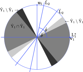
$$\hat{{\mathrm{Y}}}_{1} = {\mathrm{Y}}_{1,\hat{2}}\cap\{\mathbf{x}\in{\mathrm{B}}(\mathbf{0},1)\dvtx\hat{\theta}/2-\pi/2<\theta_{\mathbf{u}_{1},\mathbf{v}_{1}}(\mathbf{x})<\hat{\theta}/2\},$$ (56)

$$\tilde{{\mathrm{Y}}}_{1} = {\mathrm{Y}}_{1,\hat{2}}\cap\{\mathbf{x}\in{\mathrm{B}}(\mathbf{0},1)\dvtx\tilde{\theta}/2-\pi/2<\theta_{\mathbf{u}_{1},\mathbf{v}_{1}}(\mathbf{x})<\tilde{\theta}/2\}.$$ (57)

Figure 3 clarifies (56) and (57) in the special case where $d=1$ and $K=2$.

Combining (56) and (57) with the definition of $\mathbf{D}_{\mathrm{L},\mathbf{x},p}$ in (40), we obtain that

$$\quad\hat{{\mathrm{Y}}}_{1}\setminus\tilde{{\mathrm{Y}}}_{1}\subset\bigl{\{}\mathbf{x}\in{\mathrm{B}}(\mathbf{0},1)\dvtx\mathbf{v}_{1}^{T}\mathbf{x}\mathbf{x}^{T}\mathbf{u}_{1}\equiv\operatorname{dist}(\mathbf{x},\mathrm{L}^{*}_{1})^{(2-p)}\mathbf{v}_{1}^{T}\mathbf{D}_{\mathrm{L}^{*}_{1},\mathbf{x},p}\mathbf{u}_{1}>0\bigr{\}}$$ (58)

and

$$\quad\tilde{{\mathrm{Y}}}_{1}\setminus\hat{{\mathrm{Y}}}_{1}\subset\bigl{\{}\mathbf{x}\in{\mathrm{B}}(\mathbf{0},1)\dvtx\mathbf{v}_{1}^{T}\mathbf{x}\mathbf{x}^{T}\mathbf{u}_{1}\equiv\operatorname{dist}(\mathbf{x},\mathrm{L}^{*}_{1})^{(2-p)}\mathbf{v}_{1}^{T}\mathbf{D}_{\mathrm{L}^{*}_{1},\mathbf{x},p}\mathbf{u}_{1}<0\bigr{\}}.$$ (59)

It follows from Lemma 4.2 that $\mathcal{L}_{D}((\tilde{{\mathrm{Y}}}_{1}\setminus\hat{{\mathrm{Y}}}_{1})\cup(\hat{{\mathrm{Y}}}_{1}\setminus\tilde{{\mathrm{Y}}}_{1}))>0$ and, consequently, for any $r>0$, $\mathcal{L}_{D}({\mathrm{B}}(\mathbf{0},r)\cap((\tilde{{\mathrm{Y}}}_{1}\setminus\hat{{\mathrm{Y}}}_{1})\cup(\hat{{\mathrm{Y}}}_{1}\setminus\tilde{{\mathrm{Y}}}_{1})))>0$ (indeed, if $\mathbf{x}\in{\mathrm{Y}}_{1}$, then $c\cdot\mathbf{x}\in{\mathrm{Y}}_{1}$ for any $0<c<1/\|\mathbf{x}\|$; thus, the distribution in the latter inequality is just a scaling by $r^{D}$ of the distribution in the former one). Since there exists $r>0$ such that the restriction of $\mathcal{L}_{D}$ to ${\mathrm{B}}(\mathbf{0},r)$ is absolutely continuous with respect to $\mu_{0}$, we also have that $\mu_{0}({\mathrm{B}}(\mathbf{0},r)\cap((\tilde{{\mathrm{Y}}}_{1}\setminus\hat{{\mathrm{Y}}}_{1})\cup(\hat{{\mathrm{Y}}}_{1}\setminus\tilde{{\mathrm{Y}}}_{1})))>0$. However, this contradicts (55), (58) and (59), that is, it proves (4.4.1) and therefore the theorem in the current special case.

4.4.3 The case $d=D-1$

We note that the proof of the above case ($d=1$) can be adapted to the case where $d=D-1$. This is done by letting $\mathbf{v}_{1}$ be one of the two unit vectors spanning $\mathrm{L}^{*}_{1}\cap(\mathrm{L}^{*}_{1}\cap\mathrm{L}^{*}_{2})^{\perp}$ [note that $\dim(\mathrm{L}^{*}_{1})=D-1$ and $\dim(\mathrm{L}^{*}_{1}\cap\mathrm{L}^{*}_{2})=d-2$ so that $\dim(\mathrm{L}^{*}_{1}\cap(\mathrm{L}^{*}_{1}\cap\mathrm{L}^{*}_{2})^{\perp})=1$] and $\mathbf{u}_{1}$ be the unit vector of $(\mathrm{L}^{*}_{1}+\mathrm{L}^{*}_{2})\cap\mathrm{L}_{1}^{\perp}$ with a similar orientation as in the case where $d=1$.

4.5 Conclusion: The case where $d\neq 1$ and $d\neq D-1$

4.5.1 Reduction of (4.3.2) using additional condition on the Grassmannian

The following reduction is analogous to the one of Section 4.4.1. Denoting by $B(\mathbb{R}^{D},\mathbb{R}^{D})$ the space of linear operators from $\mathbb{R}^{D}$ to itself, we define

$$\Omega_{1} = \{(P_{1},P_{2})\in B(\mathbb{R}^{D},\mathbb{R}^{D})^{2}\dvtx\exists\mathrm{L}\in\mathrm{G}(D,d)\mbox{ not orthogonal to }\mathrm{L}^{*}_{1},$$

$$\hskip 23.5pt\mbox{s.t. }\dim(\mathrm{L}^{*}_{1}\ominus\mathrm{L})>1,P_{\mathrm{L}^{*}_{1}}^{T}P_{\mathrm{L}}P_{\mathrm{L}^{*}_{1}}=P_{1},P_{\mathrm{L}^{*}_{1}}^{\perp T}P_{\mathrm{L}}P^{\perp}_{\mathrm{L}^{*}_{1}}=P_{2}\}$$

and the distribution $\omega_{1}$ on $\Omega_{1}$ as follows: for any set $\mathrm{A}\subseteq\Omega_{1}$,

$$\omega_{1}(\mathrm{A})=\gamma_{D,d}\bigl{(}\mathrm{L}\in\mathrm{G}(D,d)\dvtx(P_{\mathrm{L}^{*}_{1}}^{T}P_{\mathrm{L}}P_{\mathrm{L}^{*}_{1}},P_{\mathrm{L}^{*}_{1}}^{\perp T}P_{\mathrm{L}}P^{\perp}_{\mathrm{L}^{*}_{1}})\in\mathrm{A}\bigr{)}.$$

Using this notation, we reduce (4.3.2) as follows:

$$\gamma_{D,d}\Bigl{(}\mathrm{L}^{*}_{2}\in\mathrm{G}(D,d)\dvtx\mathrm{L}^{*}_{1}\not\perp\mathrm{L}^{*}_{2},\operatorname{dim}(\mathrm{L}^{*}_{1}\cap\mathrm{L}^{*\perp}_{2})>1,$$

$$\hphantom{\gamma_{D,d}\Bigl{(}}\min_{1\leq i\neq j\leq K}\theta_{d^{*}}(\mathrm{L}^{*}_{i},\mathrm{L}^{*}_{j})>0,\mathop{\arg\min}_{2\leq i\leq K}\theta_{d^{*}}(\mathrm{L}^{*}_{1},\mathrm{L}^{*}_{i})=2,$$

(60)

$$\hphantom{\gamma_{D,d}\Bigl{(}}\mathbb{E}_{\mu_{0}}\bigl{(}I(\mathbf{x}\in{\mathrm{Y}}_{1})\mathbf{D}_{\mathrm{L}^{*}_{1},\mathbf{x},p}\bigr{)}=\mathbf{0}|$$

$$\hphantom{\gamma_{D,d}\Bigl{(}}\hskip 31.0pt(P_{\mathrm{L}^{*}_{1}}^{T}P_{\mathrm{L}^{*}_{2}}P_{\mathrm{L}^{*}_{1}},P_{\mathrm{L}^{*}_{1}}^{\perp T}P_{\mathrm{L}^{*}_{2}}P^{\perp}_{\mathrm{L}^{*}_{1}})=(P_{1},P_{2})\in\Omega_{1}\Bigr{)}=0.$$

Indeed,

$$\gamma_{D,d}\Bigl{(}\mathrm{L}^{*}_{2}\in\mathrm{G}(D,d)\dvtx\min_{1\leq i\neq j\leq K}\theta_{d^{*}}(\mathrm{L}^{*}_{i},\mathrm{L}^{*}_{j})>0,\mathop{\arg\min}_{2\leq i\leq K}\theta_{d^{*}}(\mathrm{L}^{*}_{1},\mathrm{L}^{*}_{i})=2,$$

$$\hskip 193.5pt\mathbb{E}_{\mu_{0}}\bigl{(}I(\mathbf{x}\in{\mathrm{Y}}_{1})\mathbf{D}_{\mathrm{L}^{*}_{1},\mathbf{x},p}\bigr{)}=\mathbf{0}\Bigr{)}$$

$$\qquad\leq\int_{\Omega_{1}}\gamma_{D,d}\bigl{(}\mathrm{L}^{*}_{2}\dvtx\mathrm{L}^{*}_{1}\mbox{ is not orthogonal to }\mathrm{L}^{*}_{2},$$

$$\qquad\hphantom{\leq\int_{\Omega_{1}}\gamma_{D,d}\bigl{(}}\dim(\mathrm{L}^{*}_{1}\ominus\mathrm{L}^{*}_{2})>1,\min_{1\leq i\neq j\leq K}\theta_{d^{*}}(\mathrm{L}^{*}_{i},\mathrm{L}^{*}_{j})>0,$$

$$\qquad\hphantom{\leq\int_{\Omega_{1}}\gamma_{D,d}\bigl{(}}\mathop{\arg\min}_{2\leq i\leq K}\theta_{d^{*}}(\mathrm{L}^{*}_{1},\mathrm{L}^{*}_{i})=2,$$

$$\qquad\hphantom{\leq\int_{\Omega_{1}}\gamma_{D,d}\bigl{(}}\mathbb{E}_{\mu_{0}}\bigl{(}I(\mathbf{x}\in{\mathrm{Y}}_{1})\mathbf{D}_{\mathrm{L}^{*}_{1},\mathbf{x},p}\bigr{)}=\mathbf{0}|$$

$$\qquad\hphantom{\leq\int_{\Omega_{1}}\gamma_{D,d}\bigl{(}}\hskip 7.0pt(P_{\mathrm{L}^{*}_{1}}^{T}P_{\mathrm{L}^{*}_{2}}P_{\mathrm{L}^{*}_{1}},P_{\mathrm{L}^{*}_{1}}^{\perp T}P_{\mathrm{L}^{*}_{2}}P^{\perp}_{\mathrm{L}^{*}_{1}})=(P_{1},P_{2})\in\Omega_{1}\bigr{)}\,{\mathrm{d}}(\omega_{1}(P_{1},P_{2}))$$

$$\qquad\quad{}+\gamma_{D,d}\bigl{(}\mathrm{L}^{*}_{2}\in\mathrm{G}(D,d)\dvtx\dim(\mathrm{L}^{*}_{1}\ominus\mathrm{L}^{*}_{2})\leq 1\mbox{, or }\mathrm{L}^{*}_{2}\perp\mathrm{L}^{*}_{1}\bigr{)}=0+0=0.\vspace*{-1pt}$$

4.5.2 Bulk of the proof

We prove (4.5.1) by using the following two lemmata, which are proved below (Sections 4.5.3 and 4.5.4).

Lemma 4.3

If $\dim(\mathrm{L}^{*}_{1}\ominus\mathrm{L}^{*}_{2})\geq 2$ and $\mathrm{L}^{*}_{1}$ is not orthogonal to $\mathrm{L}^{*}_{2}$, then the set

$$\mathrm{Z}=\{\mathrm{L}\in\mathrm{G}(D,d)\dvtx P_{\mathrm{L}^{*}_{1}}(P_{\mathrm{L}^{*}_{2}}-P_{\mathrm{L}})P_{\mathrm{L}^{*}_{1}}=0,P^{\perp}_{\mathrm{L}^{*}_{1}}(P_{{\mathrm{L}}^{*}_{2}}-P_{\mathrm{L}})P^{\perp}_{\mathrm{L}^{*}_{1}}=0\}\vspace*{-1pt}$$

is infinite.

Lemma 4.4

If $\tilde{\mathrm{L}}_{2},\hat{\mathrm{L}}_{2}\,{\in}\,\mathrm{G}(D,d)$ satisfy $\tilde{\mathrm{L}}_{2}\,{\neq}\,\hat{\mathrm{L}}_{2}$, $\theta_{d^{*}}(\hat{\mathrm{L}}_{2},\mathrm{L}^{*}_{1})\vee\theta_{d^{*}}(\mathrm{L}^{*}_{2},\mathrm{L}^{*}_{1})\leq\min_{3\leq i\leq K}\theta_{d^{*}}(\mathrm{L}^{*}_{i},\mathrm{L}^{*}_{1})$, $P_{\mathrm{L}^{*}_{1}}(P_{\hat{\mathrm{L}}_{2}}-P_{\tilde{\mathrm{L}}_{2}})P_{\mathrm{L}^{*}_{1}}=0$ and $P^{\perp}_{\mathrm{L}^{*}_{1}}(P_{\hat{\mathrm{L}}_{2}}-P_{\tilde{\mathrm{L}}_{2}})P^{\perp}_{\mathrm{L}^{*}_{1}}=0$, then either $\hat{\mathrm{L}}_{2}$ or $\tilde{\mathrm{L}}_{2}$ will not satisfy the condition in (4.5.1).

To conclude (4.5.1), we rewrite it as follows: $\gamma_{D,d}(A|B)=0$, where $A$ and $B$ are clear from the context. We note that Lemma 4.3 implies that there are infinitely many subspaces $\mathrm{L}^{*}_{2}$ in $B$. On the other hand, Lemma 4.4 implies that there is only one subspace $\mathrm{L}^{*}_{2}$ in $A$. These observations clearly prove (4.5.1). We remark that the idea of this proof is somewhat similar to that of the previous case where $d=1$ or $d=D-1$. In this case, Lemma 4.3 is analogous to the fact that there is a degree of freedom in choosing $\mathrm{L}_{2}^{*}$ in (4.4.1) [since we can choose any $\theta_{d^{*}}(\mathrm{L}_{1}^{*},\mathrm{L}_{2}^{*})<\min_{3\leq i\leq K}\theta_{d^{*}}(\mathrm{L}_{1}^{*},\mathrm{L}_{i}^{*})$]. Moreover, Lemma 4.4 is analogous to the fact that there were not two subspaces $\hat{\mathrm{L}}_{2}$ and $\tilde{\mathrm{L}}_{2}$ satisfying the underlying condition of (4.4.1).

4.5.3 Proof of Lemma 4.3

We denote $\tilde{\mathrm{L}}_{1}={\mathrm{L}^{*}_{1}}\ominus{(\mathrm{L}^{*}_{1}\cap\mathrm{L}^{*}_{2})}$ and $\tilde{\mathrm{L}}_{2}=\mathrm{L}^{*}_{2}\ominus(\mathrm{L}^{*}_{1}\cap\mathrm{L}^{*}_{2})$. The idea of the proof is to construct a one-to-one function $g\dvtx S^{D-1}\cap\tilde{\mathrm{L}}_{2}\rightarrow\mathrm{Z}$. Then, using this function and the fact that $\operatorname{dim}(\tilde{\mathrm{L}}_{2})=\operatorname{dim}(\mathrm{L}^{*}_{1})-\operatorname{dim}(\mathrm{L}^{*}_{2}\cap\mathrm{L}^{*}_{1})\geq 2$, we conclude that $\mathrm{Z}$, which contains $g(S^{D-1}\cap\tilde{\mathrm{L}}_{2})$, is infinite.

For any $\mathbf{u}_{0}\in S^{D-1}\cap\tilde{\mathrm{L}}_{2}$, we arbitrarily fix $\mathbf{v}_{0}=\mathbf{v}_{0}(\mathbf{u}_{0})$ as one of the two unit vectors spanning $\tilde{\mathrm{L}}_{1}\cap(\tilde{\mathrm{L}}_{2}\ominus\operatorname{Sp}(\mathbf{u}_{0}))^{\perp}$. The vector $\mathbf{v}_{0}$ exists since

$$\dim\bigl{(}\tilde{\mathrm{L}}_{1}\cap\bigl{(}\tilde{\mathrm{L}}_{2}\ominus\operatorname{Sp}(\mathbf{u}_{0})\bigr{)}^{\perp}\bigr{)} \geq \dim(\tilde{\mathrm{L}}_{1})+\dim\bigl{(}\bigl{(}\tilde{\mathrm{L}}_{2}\ominus\operatorname{Sp}(\mathbf{u}_{0})\bigr{)}^{\perp}\bigr{)}-D$$

$$= d+(D-d+1)-D=1.$$

We define the function $g$ as follows:

$$g(\mathbf{u}_{0})=\operatorname{Sp}\bigl{(}\mathbf{u}_{0}-2(\mathbf{v}_{0}^{T}\mathbf{u}_{0})\mathbf{v}_{0},\mathrm{L}^{*}_{2}\ominus\operatorname{Sp}(\mathbf{u}_{0})\bigr{)}.$$

We first claim that the image of $g$ is contained in $\mathrm{Z}$. Indeed, we note that

$$\quad P_{g(\mathbf{u}_{0})}-P_{\mathrm{L}^{*}_{2}} = \bigl{(}\mathbf{u}_{0}-2(\mathbf{v}_{0}^{T}\mathbf{u}_{0})\mathbf{v}_{0}\bigr{)}^{T}\bigl{(}\mathbf{u}_{0}-2(\mathbf{v}_{0}^{T}\mathbf{u}_{0})\mathbf{v}_{0}\bigr{)}-\mathbf{u}_{0}^{T}\mathbf{u}_{0}$$

$$= -2(\mathbf{v}_{0}^{T}\mathbf{u}_{0})\bigl{(}\mathbf{v}_{0}^{T}\bigl{(}\mathbf{u}_{0}-(\mathbf{v}_{0}^{T}\mathbf{u}_{0})\mathbf{v}_{0}\bigr{)}+\bigl{(}\mathbf{u}_{0}-(\mathbf{v}_{0}^{T}\mathbf{u}_{0})\mathbf{v}_{0}\bigr{)}^{T}\mathbf{v}_{0}\bigr{)}.$$

Combining (4.5.3) with the following two facts: $\mathbf{v}_{0}\in\mathrm{L}^{*}_{1}$ and $\mathbf{u}_{0}-(\mathbf{v}_{0}^{T}\mathbf{u}_{0})\mathbf{v}_{0}\in\mathrm{L}^{*\perp}_{1}$, we obtain that $g(\mathbf{u}_{0})\in\mathrm{Z}$.

At last, we prove that $g$ is one-to-one and thus conclude the proof. If, on the contrary, there exist $\mathbf{u}_{1}$, $\mathbf{u}_{2}\in S^{D-1}\cap\tilde{\mathrm{L}}_{2}$ such that $\mathbf{u}_{1}\neq\mathbf{u}_{2}$ and $g(\mathbf{u}_{1})=g(\mathbf{u}_{2})$, then $g(\mathbf{u}_{1})=\operatorname{Sp}(g(\mathbf{u}_{1}),g(\mathbf{u}_{2}))\supseteq(\mathrm{L}^{*}_{2}\ominus\operatorname{Sp}(\mathbf{u}_{1}))+(\mathrm{L}^{*}_{2}\ominus\operatorname{Sp}(\mathbf{u}_{2}))\supseteq\mathrm{L}^{*}_{2}$. Since $\dim(g(\mathbf{u}_{1}))=\dim(\mathrm{L}^{*}_{2})$, we conclude that $g(\mathbf{u}_{1})=\mathrm{L}^{*}_{2}$. On the other hand, we claim that for any $\mathbf{u}_{0}\in S^{D-1}\cap\tilde{\mathrm{L}}_{2}\dvtx g(\mathbf{u}_{0})\neq\mathrm{L}^{*}_{2}$ and thus obtain a contradiction. Indeed, since $\mathbf{u}_{0}\in\tilde{\mathrm{L}}_{2}$, $\mathbf{v}_{0}\in\tilde{\mathrm{L}}_{1}$ and $\mathrm{L}^{*}_{1}$ is not orthogonal to $\mathrm{L}^{*}_{2}$, we have that $\mathbf{v}_{0}^{T}\mathbf{u}_{0}\neq 0$ and, consequently, $\mathbf{u}_{0}-(\mathbf{v}_{0}^{T}\mathbf{u}_{0})\mathbf{v}_{0}\neq\mathbf{u}_{0}$. Applying the latter observation in (4.5.3), we obtain that $P_{g(\mathbf{u}_{0})}\neq P_{\mathrm{L}^{*}_{2}}$ and, consequently, $g(\mathbf{u}_{0})\neq\mathrm{L}^{*}_{2}$.

4.5.4 Proof of Lemma 4.4

We assume, on the contrary, that both $\hat{\mathrm{L}}_{2}$ and $\tilde{\mathrm{L}}_{2}$ satisfy the underlying condition of (4.3.2) and conclude a contradiction.

We arbitrarily fix here $\mathbf{x}\in\hat{{\mathrm{Y}}}_{1}\setminus\tilde{{\mathrm{Y}}}_{1}$ [using the notation of (41)]. We note that $\operatorname{dist}(\mathbf{x},\mathrm{L}^{*}_{1})<\operatorname{dist}(\mathbf{x},\hat{\mathrm{L}}_{2})$ and $\operatorname{dist}(\mathbf{x},\mathrm{L}^{*}_{1})<\arg\min_{3\leq i\leq K}\operatorname{dist}(\mathbf{x},\mathrm{L}^{*}_{i})$. Since $\mathbf{x}\notin\tilde{{\mathrm{Y}}}_{1}$, we have that $\operatorname{dist}(\mathbf{x},\mathrm{L}^{*}_{1})>\operatorname{dist}(\mathbf{x},\tilde{\mathrm{L}}_{2})$ and, thus,

$$\operatorname{dist}(\mathbf{x},\tilde{\mathrm{L}}_{2})<\operatorname{dist}(\mathbf{x},\mathrm{L}^{*}_{1})<\operatorname{dist}(\mathbf{x},\hat{\mathrm{L}}_{2}).$$ (62)

Consequently,

$$\mathbf{x}^{T}(P_{\hat{\mathrm{L}}_{2}}-P_{\tilde{\mathrm{L}}_{2}})\mathbf{x}=\operatorname{dist}(\mathbf{x},\tilde{\mathrm{L}}_{2})^{2}-\operatorname{dist}(\mathbf{x},\hat{\mathrm{L}}_{2})^{2}<0.$$ (63)

We partition $P_{\hat{\mathrm{L}}_{2}}-P_{\tilde{\mathrm{L}}_{2}}$ into four parts: $P_{\mathrm{L}^{*}_{1}}(P_{\hat{\mathrm{L}}_{2}}-P_{\tilde{\mathrm{L}}_{2}})P_{\mathrm{L}^{*}_{1}}$, $P^{\perp}_{\mathrm{L}^{*}_{1}}(P_{\hat{\mathrm{L}}_{2}}-P_{\tilde{\mathrm{L}}_{2}})P^{\perp}_{\mathrm{L}^{*}_{1}}$, $P_{\mathrm{L}^{*}_{1}}(P_{\hat{\mathrm{L}}_{2}}-P_{\tilde{\mathrm{L}}_{2}})P^{\perp}_{\mathrm{L}^{*}_{1}}$ and $P^{\perp}_{\mathrm{L}^{*}_{1}}(P_{\hat{\mathrm{L}}_{2}}-P_{\tilde{\mathrm{L}}_{2}})P_{\mathrm{L}^{*}_{1}}$. The first two are zero, and the last two are adjoint to each other; we thus only consider $P_{\mathrm{L}^{*}_{1}}(P_{\hat{\mathrm{L}}_{2}}-P_{\tilde{\mathrm{L}}_{2}})P^{\perp}_{\mathrm{L}^{*}_{1}}$. Let its SVD be

$$P_{\mathrm{L}^{*}_{1}}(P_{\hat{\mathrm{L}}_{2}}-P_{\tilde{\mathrm{L}}_{2}})P^{\perp}_{\mathrm{L}^{*}_{1}}=\mathbf{U}\bolds{\Sigma}\mathbf{V}=\sum_{i=1}^{d}\sigma_{i}\mathbf{u}_{i}\mathbf{v}_{i}^{T}.$$ (64)

We can express the SVD of $P_{\hat{\mathrm{L}}_{2}}-P_{\tilde{\mathrm{L}}_{2}}$ using (64) and the partition above as follows:

$$P_{\hat{\mathrm{L}}_{2}}-P_{\tilde{\mathrm{L}}_{2}}=\sum_{i=1}^{d}\sigma_{i}(\mathbf{u}_{i}\mathbf{v}_{i}^{T}+\mathbf{v}_{i}\mathbf{u}_{i}^{T}).$$ (65)

Combining (63) and (65), we obtain that

$$\sum_{i=1}^{n}\sigma_{i}\mathbf{u}^{T}_{i}\mathbf{x}\mathbf{x}^{T}\mathbf{v}_{i}=\mathbf{x}^{T}\Biggl{(}\sum_{i=1}^{n}\sigma_{i}(\mathbf{u}_{i}\mathbf{v}^{T}_{i}+\mathbf{v}_{i}\mathbf{u}^{T}_{i})\Biggr{)}\mathbf{x}/2<0.$$ (66)

We define a function $f\dvtx\mathbb{R}^{D\times D}\rightarrow\mathbb{R}$ such that for any $\mathbf{A}\in\mathbb{R}^{D\times D}\dvtx f(\mathbf{A})=\sum_{i=1}^{n}\sigma_{i}\mathbf{u}^{T}_{i}\mathbf{A}\mathbf{v}_{i}$. Using (66) and the fact that $\{\mathbf{u}_{i}\}_{i=1}^{d}\in\mathrm{L}^{*}_{1}$ and $\{\mathbf{v}_{i}\}_{i=1}^{d}\in\mathrm{L}^{*\perp}_{1}$, we deduce that

$$f(\mathbf{D}_{\mathrm{L}^{*}_{1},\mathbf{x},p}) = \operatorname{dist}(\mathbf{x},\mathrm{L}^{*}_{1})^{(p-2)}f(P_{\mathrm{L}^{*}_{1}}(\mathbf{x})P^{\perp}_{\mathrm{L}^{*}_{1}}(\mathbf{x})^{T})$$

$$= \operatorname{dist}(\mathbf{x},\mathrm{L}^{*}_{1})^{(p-2)}\sum_{i=1}^{n}\sigma_{i}\mathbf{u}^{T}_{i}P_{\mathrm{L}^{*}_{1}}(\mathbf{x})P^{\perp}_{\mathrm{L}^{*}_{1}}(\mathbf{x})^{T}\mathbf{v}_{i}$$

$$= \operatorname{dist}(\mathbf{x},\mathrm{L}^{*}_{1})^{(p-2)}\sum_{i=1}^{n}\sigma_{i}\mathbf{u}^{T}_{i}\mathbf{x}\mathbf{x}^{T}\mathbf{v}_{i}<0.$$

Similarly, for any point $\mathbf{x}\in\tilde{{\mathrm{Y}}}_{1}\setminus\hat{{\mathrm{Y}}}_{1}$,

$$f(\mathbf{D}_{\mathrm{L}^{*}_{1},\mathbf{x},p})>0.$$ (68)

Combining (4.4.2), (4.5.4), (68), Lemma 4.2 and the linearity of $f$, we conclude the following contradiction establishing the current lemma:

$$\quad 0 = f\bigl{(}\mathbb{E}_{\mu_{0}}\bigl{(}I(\mathbf{x}\in\tilde{{\mathrm{Y}}}_{1}\setminus\hat{{\mathrm{Y}}}_{1})\mathbf{D}_{\mathrm{L}^{*}_{1},\mathbf{x},p}\bigr{)}-\mathbb{E}_{\mu_{0}}\bigl{(}I(\mathbf{x}\in\hat{{\mathrm{Y}}}_{1}\setminus\tilde{{\mathrm{Y}}}_{1})\mathbf{D}_{\mathrm{L}^{*}_{1},\mathbf{x},p}\bigr{)}\bigr{)}$$

$$= f\bigl{(}\mathbb{E}_{\mu_{0}}\bigl{(}I(\mathbf{x}\in\tilde{{\mathrm{Y}}}_{1}\setminus\hat{{\mathrm{Y}}}_{1})\mathbf{D}_{\mathrm{L}^{*}_{1},\mathbf{x},p}\bigr{)}\bigr{)}-f\bigl{(}\mathbb{E}_{\mu_{0}}\bigl{(}I(\mathbf{x}\in\hat{{\mathrm{Y}}}_{1}\setminus\tilde{{\mathrm{Y}}}_{1})\mathbf{D}_{\mathrm{L}^{*}_{1},\mathbf{x},p}\bigr{)}\bigr{)}$$

$$> 0.\vspace*{-3pt}$$

4.5.5 Remark on the sizes of $\delta_{0}$ and $\kappa_{0}$

The constants $\delta_{0}$ and $\kappa_{0}$ depend on other parameters of the underlying weak HLM model, in particular, the underlying subspaces $\{\mathrm{L}^{*}_{i}\}_{i=1}^{K}$. For example, one can bound both $\kappa_{0}$ and $\delta_{0}$ from below by the following number:

$$\max_{1\leq i\leq K}\Bigl{(}\mathbb{E}_{\mu}\bigl{(}e_{l_{p}}(\mathbf{x},\mathrm{L}_{i}^{*})I(\mathbf{x}\in{\mathrm{Y}}_{i})\bigr{)}-\min_{\mathrm{L}\in\mathrm{G}(D,d)}\mathbb{E}_{\mu}\bigl{(}e_{l_{p}}(\mathbf{x},\mathrm{L})I(\mathbf{x}\in{\mathrm{Y}}_{i})\bigr{)}\Bigr{)}\big{/}(4p).$$

If $p\geq 2$, then a simpler lower bound on both $\kappa_{0}$ and $\delta_{0}$ is

$$\frac{\|{\max_{1\leq i\leq K}\mathbb{E}_{\mu}}(\mathbf{D}_{\mathrm{L}^{*}_{1},\mathbf{x},p}I(\mathbf{x}\in{\mathrm{Y}}_{i}))\|_{2}^{2}}{pdD2^{p+5}}.$$

5 Discussion

We studied the effectiveness of $l_{p}$ minimization for recovering (or nearly recovering) all underlying $K$ subspaces for i.i.d. samples from two different types of HLM distributions. In particular, we demonstrated a phase transition phenomenon around $p=1$.

We discuss here implications, extensions and limitations of this theory as well as some open directions.

5.1 Obstacles for convex recovery of multiple subspaces

There are some recent methods for robust single subspace recovery by convex optimization (see, e.g., wrightrobustpca09 ). Such methods minimize a real-valued convex function $h$ on a convex set $\mathbb{H}$ (e.g., set of matrices), which can be mapped on $\mathrm{G}(D,d)$. However, such a minimization cannot be done for multiple subspaces. Indeed, in that case one must minimize a multivariate function $h\dvtx\mathbb{H}^{K}\rightarrow\mathbb{R}$ for convex $\mathbb{H}$. Clearly, the function $h$ must be invariant to permutations of coordinates. Let $g$ be a mapping of $\mathbb{H}$ onto $\mathrm{G}(D,d)$. It follows from the assumption that the minimization of $h$ leads to the underlying subspaces $\{\mathrm{L}_{i}^{*}\}_{i=1}^{K}$ and the permutation-invariance of $h$ that the set of minimizers of $h$ coincides with all permutations of $\hat{\mathbf{x}}_{1},\hat{\mathbf{x}}_{2},\ldots,\hat{\mathbf{x}}_{K}$, where $\hat{\mathbf{x}}_{i}\in g^{-1}(\mathrm{L}_{i}^{*})$ for all $1\leq i\leq K$. Since $h$ is convex, $({\sum_{i=1}^{K}\hat{\mathbf{x}}_{i}}/{K},\ldots,{\sum_{i=1}^{K}\hat{\mathbf{x}}_{i}}/{K})$ is also a minimizer of $h$. Consequently, ${\sum_{i=1}^{K}\hat{\mathbf{x}}_{i}}/{K}\in g^{-1}(\mathrm{L}_{j}^{*})$ for all $1\leq j\leq K$, and, thus, $g({\sum_{i=1}^{K}\hat{\mathbf{x}}_{i}}/{K})=\mathrm{L}_{1}^{*}=\cdots=\mathrm{L}_{K}^{*}$, which is a contradiction.

Furthermore, a minimization on $\mathrm{G}(D,d)^{K}$ cannot even be geodesically convex. Indeed, the maximum of a geodesically convex function on a compact, geodesically convex set is attained on the boundary. However, $\mathrm{G}(D,d)^{K}$ is compact, geodesically convex and has no boundary, so any function defined on $\mathrm{G}(D,d)^{K}$ is not geodesically convex.

5.2 Implications for a single subspace recovery

In lprecoverypart111 , we discussed the recovery of a single subspace. Theorems 1.1 and 1.2 apply to this case when $K=1$. Unlike lprecoverypart111 which assumed that $\mu_{0}$ was spherically symmetric (while having possibly additional “outliers” along other subspaces, distributed according to $\{\mu_{i}\}_{i=2}^{K}$), here we have a very weak requirement from $\mu_{0}$ (which represents all outliers). However, here there is a strong restriction on the fraction of outliers, $\alpha_{0}$, whereas in lprecoverypart111 there was no requirement, except for $\alpha_{0}<1$.

5.3 Extending our theory to more general distributions

In Theorems 1.1 and 1.2, the strict spherical symmetry of $\{\mu_{i}\}_{i=1}^{K}$ (within $\{\mathrm{L}_{i}\}_{i=1}^{K}$, resp.) can be replaced by approximate spherical symmetry of $\{\mu_{i}\}_{i=1}^{K}$. That is, for each $1\leq i\leq K$ and $\mathrm{L}_{i}$ and $\mu_{i}$ as before, we form a new distribution $\mu_{i}^{\prime}$, with the same support as $\mu_{i}$ such that the derivative of $\mu_{i}^{\prime}$ w.r.t. $\mu_{i}$ is bounded away from $0$ and $\infty$. We then replace $\mu_{i}$ with $\mu_{i}^{\prime}$. This new setting will require replacing $\{\alpha_{i}\}_{i=1}^{K}$ in (6)–(8) by $\{\delta_{i}\,\alpha_{i}\}_{i=1}^{K}$, where $\delta_{i}\equiv\delta_{i}(\mu_{i}^{\prime},\mu_{i})$ for $1\leq i\leq K$ ($\delta_{i}$ is the lowest value of the derivative of $\mu_{i}^{\prime}$ w.r.t. $\mu_{i}$).

Furthermore, the boundedness of the support of the distributions $\{\mu_{i}\}_{i=0}^{K}$ can be weakened by assuming that these distributions are sub-Gaussian. Indeed, this will mainly require changing Hoeffding’s inequality with taoranmatbook , Proposition 2.1.9.

5.4 Distributions resulting in counterexamples for our theory

There are several typical cases with settings different than above, where the underlying subspaces cannot be recovered by minimizing the energy (1) for all $p>0$.

The first typical example is when there is an outlier with sufficiently large magnitude so that the minimizer of (1) contains a subspace passing through this outlier, which is different than any of the underlying subspaces. Our setting avoids such a counterexample by requiring (6). We briefly provide the idea as follows: an arbitrarily large outlier in our setting of supports within ${\mathrm{B}}(\mathbf{0},1)$ means, for example, that the outlier has magnitude one and the inliers are supported within ${\mathrm{B}}(\mathbf{0},\varepsilon)$, where $\varepsilon$ is arbitrarily small. Therefore, $\psi(\varepsilon)=1$, so that $\psi_{\mu_{1}}^{-1}({(1+(2K-1)\mu_{1}(\{\mathbf{0}\}))}/{2K})<\psi_{\mu_{1}}^{-1}(1)=\varepsilon$ and, consequently, $\tau_{0}\lessapprox\varepsilon^{p}$. In view of (6), we control the fraction of outliers as a function of $\varepsilon^{p}$. In particular, for a fixed sample size and sufficiently small $\varepsilon$, no outliers are allowed by this condition.

The second example is when the distribution of outliers lies on another subspace, $\mathrm{L}^{*}_{0}\in\mathrm{G}(D,d)$ and $\alpha_{0}>\min_{1\leq i\leq K}\alpha_{i}$, so that $\mathrm{L}^{*}_{0}$ is contained in the minimizer of (1). Our setting avoids this counterexample by assuming an upper bound on the percentage of outliers in terms of the minimal percentage of inliers [see (6)].

For the last example we assume for simplicity that $D=2$, $d=1$, $K=2$ and underlying uniform distributions (of outliers and along the two underlying lines) restricted to the unit disk. We further assume that the two lines have angles $\varepsilon$ and $-\varepsilon$ w.r.t. the $x$-axis. By choosing $\varepsilon$ sufficiently small the $x$-axis and $y$-axis provide a smaller value for the energy (1) than the underlying lines. We note that in this case (6) does not hold [due to the small size of $\operatorname{dist}_{\mathrm{G}}(\mathrm{L}^{*}_{i},\mathrm{L}^{*}_{j})$].

5.5 Another phase transition at $p=1$: Many local minima for $0<p<1$

Our previous work lprecoverypart111 , proof of Proposition 2.1, implies that if $0<p<1$ and there exist distinct subspaces $\{\mathrm{L}_{i}\}_{i=1}^{K}\subseteq\mathrm{G}(D,d)$ such that $\operatorname{Sp}({\mathcal{X}}\cap\mathrm{L}_{i})=\mathrm{L}_{i}$ for all $1\leq i\leq K$, then $\{\mathrm{L}_{i}\}_{i=1}^{K}$ is a local minimizer of the energy (1). We note that many subspaces satisfy this condition (in particular, w.o.p. $d$-subspaces spanned by randomly sampled $d$ vectors). Therefore, $l_{p}$ minimization for multiple subspaces with $0<p<1$ will often lead to plenty of local minima.

This wealth of local minima clearly does not occur when $p=1$ (or $p\geq 1$). It will be interesting, though difficult, to carefully analyze the number and depth of local minima for $p\geq 1$.

5.6 The case of affine subspaces

Our analysis was restricted to linear subspaces, though we believe that it can be extended to affine subspaces. Indeed, we can consider the affine Grassmannian Mat95 , which distinguishes between subspaces according to both their offsets with respect to the origin (i.e., distances to closest linear subspaces of the same dimension) and their orientations (based on principal angles of the shifted linear subspaces). By assuming only affine subspaces intersecting a fixed ball, we can have a compact space. We can also generalize (.10) (with a different function $\psi_{\mu_{1}}$) and the estimates on $\delta_{0}$ and $\kappa_{0}$ in Section 4.5.5 to the case of affine subspaces. We remark, though, that it is not obvious whether the metric on the affine Grassmannian is relevant for our applications, since it mixes two different quantities of different units (i.e., offset values and orientations) so that one can arbitrarily weigh their contributions. Also, the common strategy of using homogenous coordinates which transform $d$-dimensional affine subspaces in $\mathbb{R}^{D}$ to $(d+1)$-dimensional linear subspaces in $\mathbb{R}^{D+1}$ is not useful to us since it distorts the structure of both noise and outliers.

The minimization of the energy (1) over affine subspaces seems to result in more local minima than in the linear case, which can partially explain why numerical heuristics for minimizing (1) do not perform as well with affine subspaces as they do with linear ones. We are interested in further explanation of this phenomenon.

5.7 The case of mixed dimensions

It will be interesting to try to extend our analysis to linear subspaces of mixed dimensions $d_{1},\ldots,d_{K}$, known in advance. We believe that it is possible to extend Theorem 1.1 and its proof to this case. For this purpose, we suggest using the same distance for subspaces of the same dimension and defining the distance $\operatorname{dist}_{\mathrm{G}}(\mathrm{L}_{1},\mathrm{L}_{2})$ between linear subspaces $\mathrm{L}_{1}$ and $\mathrm{L}_{2}$ of different dimensions (with some abuse of notation) as follows: if $\dim(\mathrm{L}_{1})<\dim(\mathrm{L}_{2})$, then $\operatorname{dist}_{\mathrm{G}}(\mathrm{L}_{1},\mathrm{L}_{2})=\min_{\mathrm{L}\in\mathrm{L}_{2},\dim(\mathrm{L})=\dim(\mathrm{L}_{1})}\operatorname{dist}_{\mathrm{G}}(\mathrm{L}_{1},\mathrm{L})$.

5.8 Further performance guarantees for $l_{p}$-based HLM algorithms

We are interested in extending our theory to analyze heuristics (like the $K$-subspaces) which try to minimize the $l_{p}$ energy of (1) in practice.

5.9 Asymptotic rates of convergence and sample complexity

In Section 3.2 we demonstrated simple instances when noise is present and one cannot asymptotically recover the underlying subspaces by $l_{p}$ minimization for all $p>0$. One may still inquire about the existence of asymptotic limit different than the underlying subspaces and quantify the rate of convergence (depending on the mixture model parameters) to that limit. That is, assume that $\{\hat{\mathrm{L}}_{1},\hat{\mathrm{L}}_{2}\}$ is the minimizer of $\mathbb{E}_{\mu}(l_{p}(\mathbf{x},\mathrm{L}_{1},\mathrm{L}_{2}))$ and $\{\hat{\mathrm{L}}_{1}^{N},\hat{\mathrm{L}}_{2}^{N}\}$ is the minimizer of $\mathbb{E}_{\mu_{N}}(l_{p}(\mathbf{x},\mathrm{L}_{1},\mathrm{L}_{2}))$, where $\mu_{N}$ is an empirical distribution of i.i.d. sample of $N$ points from $\mu$. We first ask whether $\operatorname{dist}(\{\hat{\mathrm{L}}_{1},\hat{\mathrm{L}}_{2}\},\{\hat{\mathrm{L}}_{1}^{N},\hat{\mathrm{L}}_{2}^{N}\})\rightarrow 0$ as $N\rightarrow\infty$. If true, then we ask about the asymptotic rates of convergence. This will then allow a definition of a sample complexity for multiple subspaces as the number of samples required to achieve a prediction error within $\varepsilon$ of the exact recovery of the $K$ $d$-subspaces.

Appendix: Supplementary details

.10 Proof of Lemma 2.1

We will use the following inequality for any $1\leq j\leq K$, which is proved in lprecoverypart111 , Section A.1.1:

$$\mu_{1}\bigl{(}\mathbf{x}\in{\mathrm{B}}(\mathbf{0},1)\cap\mathrm{L}^{*}_{1}\dvtx\operatorname{dist}(\mathbf{x},\hat{\mathrm{L}}_{j})<\beta\operatorname{dist}_{\mathrm{G}}(\mathrm{L}^{*}_{1},\hat{\mathrm{L}}_{j})\bigr{)}$$

(70)

$$\qquad\leq\psi_{\mu_{1}}\biggl{(}\frac{\pi\sqrt{d}}{2}\beta\biggr{)}\qquad\forall\beta>0.$$

We denote $\beta_{1}\,{=}\,\frac{2}{\pi\sqrt{d}}\psi_{\mu_{1}}^{-1}(\frac{1+(2K-1)\mu_{1}(\{\mathbf{0}\})}{2K})$ (the existence of $\psi_{\mu_{1}}^{-1}(\frac{1+(2K-1)\mu_{1}(\{\mathbf{0}\})}{2K})$ follows the same proof as in lprecoverypart111 , Section A.1.1) and combine (.10) with the fact that $\operatorname{dist}_{\mathrm{G}}(\mathrm{L}^{*}_{1},\hat{\mathrm{L}}_{j})\geq\varepsilon$ for any $1\leq j\leq K$ to obtain that

$$\mu_{1}\bigl{(}\mathbf{x}\in{\mathrm{B}}(\mathbf{0},1)\cap\mathrm{L}^{*}_{1}\setminus\{\mathbf{0}\}\dvtx\operatorname{dist}(\mathbf{x},\hat{\mathrm{L}}_{1})<\beta_{1}\varepsilon\bigr{)}$$

$$\qquad=\mu_{1}\bigl{(}\mathbf{x}\in{\mathrm{B}}(\mathbf{0},1)\cap\mathrm{L}^{*}_{1}\setminus\{\mathbf{0}\}\dvtx\operatorname{dist}(\mathbf{x},\hat{\mathrm{L}}_{1})<\beta_{1}\operatorname{dist}_{\mathrm{G}}(\mathrm{L}^{*}_{1},\hat{\mathrm{L}}_{1})\bigr{)}$$

$$\qquad\leq\frac{1+(2K-1)\mu_{1}(\{\mathbf{0}\})}{2K}-\mu(\{\mathbf{0}\})$$

$$\qquad=\frac{1-\mu_{1}(\{\mathbf{0}\})}{2K}.$$

Consequently,

$$\mu_{1}\Biggl{(}\mathbf{x}\in{\mathrm{B}}(\mathbf{0},1)\cap\mathrm{L}^{*}_{1}\dvtx\operatorname{dist}\Biggl{(}\mathbf{x},\bigcup_{j=1}^{K}\hat{\mathrm{L}}_{1}\Biggr{)}\geq\beta_{1}\varepsilon\Biggr{)}$$

$$\qquad\geq 1-\mu(\{\mathbf{0}\})-\sum_{i=1}^{K}\mu_{1}\bigl{(}\mathbf{x}\in{\mathrm{B}}(\mathbf{0},1)\cap\mathrm{L}^{*}_{1}\setminus\{\mathbf{0}\}\dvtx\operatorname{dist}(\mathbf{x},\hat{\mathrm{L}}_{i})<\beta_{1}\varepsilon\bigr{)}$$

$$\qquad\geq\bigl{(}1-\mu_{1}(\{\mathbf{0}\})\bigr{)}/2,$$

and, thus, by Chebyshev’s inequality the lemma is concluded as follows:

$$\mathbb{E}_{{\mu}_{1}}(e_{l_{p}}(\mathbf{x},\hat{\mathrm{L}}_{1})) \geq \beta_{1}^{p}\varepsilon^{p}/2$$

$$= \frac{(1-\mu_{1}(\{\mathbf{0}\}))2^{p-1}\psi_{\mu_{1}}^{-1}(({1+(2K-1)\mu_{1}(\{\mathbf{0}\})})/({2K}))^{p}\varepsilon^{p}}{(\pi\sqrt{d})^{p}}$$

$$= \tau_{0}\varepsilon^{p}.$$

.11 Proof of Proposition 3.1

The proof is an immediate consequence of the following inequality, which uses an arbitrary ${\mathrm{L}}_{1}\in\mathrm{G}(D,d)$ and the notation ${\mathrm{Y}}^{\prime}_{i}={\mathrm{Y}}_{i}(\mathrm{L}^{\prime}_{1},\ldots,\mathrm{L}^{\prime}_{K})$, $1\leq i\leq K$:

$$0 \leq \mathbb{E}_{\nu}(e_{l_{p}}(\mathbf{x},{\mathrm{L}}_{1},{\mathrm{L}}^{\prime}_{2},\ldots,{\mathrm{L}}^{\prime}_{K}))-\mathbb{E}_{\nu}(e_{l_{p}}(\mathbf{x},{\mathrm{L}}^{\prime}_{1},\ldots,{\mathrm{L}}^{\prime}_{K}))$$

$$\leq \mathbb{E}_{\nu}\bigl{(}I(\mathbf{x}\in{\mathrm{Y}}^{\prime}_{1})e_{l_{p}}(\mathbf{x},{\mathrm{L}}_{1})\bigr{)}+\sum_{2\leq i\leq K}\mathbb{E}_{\nu}\bigl{(}I(\mathbf{x}\in{\mathrm{Y}}^{\prime}_{i})e_{l_{p}}(\mathbf{x},{\mathrm{L}}^{\prime}_{i})\bigr{)}$$

$${}-\sum_{1\leq i\leq K}\mathbb{E}_{\nu}\bigl{(}I(\mathbf{x}\in{\mathrm{Y}}^{\prime}_{i})e_{l_{p}}(\mathbf{x},{\mathrm{L}}^{\prime}_{i})\bigr{)}$$

$$= \mathbb{E}_{\nu}\bigl{(}I(\mathbf{x}\in{\mathrm{Y}}^{\prime}_{1})e_{l_{p}}(\mathbf{x},{\mathrm{L}}_{1})\bigr{)}-\mathbb{E}_{\nu}\bigl{(}I(\mathbf{x}\in{\mathrm{Y}}^{\prime}_{1})e_{l_{p}}(\mathbf{x},{\mathrm{L}}^{\prime}_{1})\bigr{)}.$$

.12 Proof of Lemma 4.2: Geometric sensitivity

We will first show that there exists $\mathbf{x}_{0}\in{\mathrm{B}}(\mathbf{0},1)$ such that

$$\operatorname{dist}(\mathbf{x}_{0},\mathrm{L}^{*}_{1})=\operatorname{dist}(\mathbf{x}_{0},\mathrm{L}^{*}_{2})<\min_{3\leq i\leq K}\operatorname{dist}(\mathbf{x}_{0},\mathrm{L}^{*}_{i}).$$ (71)

We verify (71) in two cases: $d^{*}=d$ and $d^{*}=D-d$. We will then prove that (71) implies (47). Throughout the proof we denote the principal vectors of $\mathrm{L}^{*}_{2}$ and $\mathrm{L}^{*}_{1}$ by $\{\hat{\mathbf{v}}_{i}\}_{i=1}^{d^{*}}$ and $\{\mathbf{v}_{i}\}_{i=1}^{{d^{*}}}$, respectively.

.12.1 Part I: Proof of (71) when $d^{*}=d$

We define

$$\mathbf{x}_{0}=(\hat{\mathbf{v}}_{d^{*}}+\mathbf{v}_{d^{*}})/{\|\hat{\mathbf{v}}_{d^{*}}+\mathbf{v}_{d^{*}}\|}$$

and arbitrarily fix $i_{0}>3$ and $\mathbf{v}_{0}\in\mathrm{L}^{*}_{i_{0}}$. We will show that

$$\operatorname{ang}(\mathbf{x}_{0},\mathbf{v}_{0})>\theta_{d^{*}}(\mathrm{L}^{*}_{2},\mathrm{L}^{*}_{1})/2$$ (72)

and consequently conclude (71) as follows:

$$\operatorname{dist}(\mathbf{x}_{0},\mathrm{L}^{*}_{i_{0}}) \geq \sin(\operatorname{ang}(\mathbf{x}_{0},\mathbf{v}_{0}))>\sin\bigl{(}\theta_{d^{*}}(\mathrm{L}^{*}_{2},\mathrm{L}^{*}_{1})/2\bigr{)}=\operatorname{dist}(\mathbf{x}_{0},\mathrm{L}^{*}_{1})$$

$$= \operatorname{dist}(\mathbf{x}_{0},\mathrm{L}^{*}_{2}).$$

We can easily verify a weaker version of (72) where the inequality is not necessarily strict. Indeed, using elementary geometric estimates and the fact that the intersections of the $d$-subspaces $\{\mathrm{L}^{*}_{i}\}_{i=1}^{K}$ are empty [which follows from (45)], we obtain that

$$\qquad\operatorname{ang}(\mathbf{x}_{0},\mathbf{v}_{0}) \,{\geq}\, \operatorname{ang}(\mathbf{v}_{d^{*}},\mathbf{v}_{0})\,{-}\,\operatorname{ang}(\mathbf{v}_{d^{*}},\mathbf{x}_{0})\,{\geq}\,\theta_{d^{*}}(\mathrm{L}^{*}_{i_{0}},\mathrm{L}^{*}_{1})\,{-}\,\theta_{d^{*}}(\mathrm{L}^{*}_{2},\mathrm{L}^{*}_{1})/2$$

$$\,{\geq}\, \theta_{d^{*}}(\mathrm{L}^{*}_{2},\mathrm{L}^{*}_{1})\,{-}\,\theta_{d^{*}}(\mathrm{L}^{*}_{2},\mathrm{L}^{*}_{1})/2\,{=}\,\theta_{d^{*}}(\mathrm{L}^{*}_{2},\mathrm{L}^{*}_{1})/2.$$

At last, we show that (.12.1) cannot be an equality. Indeed, if the first inequality in (.12.1) is an equality, then $\mathbf{v}_{0}$, $\mathbf{v}_{d^{*}}$ and $\mathbf{x}_{0}$ are on a geodesic line within the sphere $S^{D-1}$. Combining this with the assumption that all other inequalities in (.12.1) are equalities, we obtain that $\operatorname{ang}(\mathbf{x}_{0},\mathbf{v}_{0})=\theta_{d^{*}}(\mathrm{L}^{*}_{2},\mathrm{L}^{*}_{1})/2=\operatorname{ang}(\mathbf{x}_{0},\mathbf{v}_{d^{*}})=\operatorname{ang}(\mathbf{x}_{0},\hat{\mathbf{v}}_{d^{*}})$. This implies that either $\mathbf{v}_{0}=\hat{\mathbf{v}}_{d^{*}}$ or $\mathbf{v}_{0}=\mathbf{v}_{d^{*}}$, which contradicts (45).

.12.2 Part II: Proof of (71) when $d^{*}=D-d$

It follows from basic dimension equalities of subspaces and (45) that for all $2\leq i\leq K\dvtx\dim(\mathrm{L}^{*}_{1}\cup\mathrm{L}^{*}_{i})=D$ and $\dim(\mathrm{L}^{*}_{1}\cap\mathrm{L}^{*}_{i})=2d-D$. We denote by $K_{0}$ the integer in $\{0,\ldots,K\}$ such that for any $3\leq i\leq K_{0}\dvtx\mathrm{L}^{*}_{1}\cap\mathrm{L}^{*}_{i}=\mathrm{L}^{*}_{1}\cap\mathrm{L}^{*}_{2}$ and for any $i>K_{0}\dvtx\mathrm{L}^{*}_{1}\cap\mathrm{L}^{*}_{i}\neq\mathrm{L}^{*}_{1}\cap\mathrm{L}^{*}_{2}$ (the existence of $K_{0}$ may require reordering of the indices of the subspaces $\{\mathrm{L}^{*}_{i}\}_{i=3}^{K}$). In order to define $\mathbf{x}_{0}$ in the current case, we let $\mathbf{x}_{1}=(\hat{\mathbf{v}}_{d^{*}}+\mathbf{v}_{d^{*}})/{\|\hat{\mathbf{v}}_{d^{*}}+\mathbf{v}_{d^{*}}\|}$, $\mathbf{x}_{2}$ be an arbitrarily fixed unit vector in $\mathrm{L}^{*}_{1}\cap(\mathrm{L}^{*}_{2}\setminus\bigcup_{K_{0}<i\leq K}\mathrm{L}^{*}_{i})$, $\varepsilon_{0}=\operatorname{dist}(\mathbf{x}_{2},\bigcup_{K_{0}<i\leq K}\mathrm{L}^{*}_{i})$ and

$$\mathbf{x}_{0}=\mathbf{x}_{2}/2+\varepsilon_{0}\mathbf{x}_{1}/5.$$

We first claim that

$$\operatorname{dist}(\mathbf{x}_{0},\mathrm{L}^{*}_{1})=\operatorname{dist}(\mathbf{x}_{0},\mathrm{L}^{*}_{2})<\min_{3\leq j\leq K_{0}}\operatorname{dist}(\mathbf{x}_{0},\mathrm{L}^{*}_{j}).$$ (74)

Indeed, we can remove $\mathrm{L}^{*}_{1}\cap\mathrm{L}^{*}_{2}$ from the subspaces $\{\mathrm{L}^{*}_{i}\}_{i=1}^{K_{0}}$ and obtain subspaces of dimension $D-d$ intersecting each other at the origin. We can then rewrite (74) by replacing $\{\mathrm{L}^{*}_{i}\}_{i=1}^{K_{0}}$ with their reduced version and $\mathbf{x}_{0}$ with $\mathbf{x}_{1}$. The argument of Section .12.1 thus proves this equation.

We conclude (71) by combining (74) with the following observation:

$$\quad\operatorname{dist}(\mathbf{x}_{0},\mathrm{L}^{*}_{1}) = \varepsilon_{0}\operatorname{dist}(\mathbf{x}_{1},\mathrm{L}^{*}_{1})/5\leq\varepsilon_{0}/5<\operatorname{dist}\biggl{(}\mathbf{x}_{2}/2,\bigcup_{K_{0}<j\leq K}\mathrm{L}^{*}_{j}\biggr{)}-\varepsilon_{0}/5$$

$$\leq \operatorname{dist}\biggl{(}\mathbf{x}_{2}/2+\varepsilon_{0}\mathbf{x}_{1}/5,\bigcup_{K_{0}<j\leq K}\mathrm{L}^{*}_{j}\biggr{)}=\min_{K_{0}<i\leq K}\operatorname{dist}(\mathbf{x}_{0},\mathrm{L}^{*}_{i}).$$

.12.3 Part III: Deriving (47) from (71) in a simple case

We note that (71) implies that

$$\mathbf{x}_{0}\in\bigl{(}{\mathrm{Y}}_{1}\cup{\mathrm{Y}}_{2}\cup(\bar{{\mathrm{Y}}}_{1}\cap\bar{{\mathrm{Y}}}_{2})\bigr{)}\cap\bigl{(}\hat{{\mathrm{Y}}}_{1}\cup\hat{{\mathrm{Y}}}_{2}\cup(\bar{\hat{{\mathrm{Y}}}}_{1}\cap\bar{\hat{{\mathrm{Y}}}}_{2})\bigr{)}$$ (76)

and, consequently,

$${\mathrm{B}}(\mathbf{x}_{0},\varepsilon)\subset\bigl{(}{\mathrm{Y}}_{1}\cup{\mathrm{Y}}_{2}\cup(\bar{{\mathrm{Y}}}_{1}\cap\bar{{\mathrm{Y}}}_{2})\bigr{)}\cap\bigl{(}\hat{{\mathrm{Y}}}_{1}\cup\hat{{\mathrm{Y}}}_{2}\cup(\bar{\hat{{\mathrm{Y}}}}_{1}\cap\bar{\hat{{\mathrm{Y}}}}_{2})\bigr{)}.$$ (77)

We will deduce here (47) from (77) in the simpler case: $\bar{\hat{{\mathrm{Y}}}}_{1}\cap\bar{\hat{{\mathrm{Y}}}}_{2}\cap{\mathrm{B}}(\mathbf{x}_{0},\varepsilon)\neq\bar{{\mathrm{Y}}}_{1}\cap\bar{{\mathrm{Y}}}_{2}\cap{\mathrm{B}}(\mathbf{x}_{0},\varepsilon)$.

Using (77) and the fact that $\mathcal{L}_{D}(\bar{{\mathrm{Y}}}_{1}\cap\bar{{\mathrm{Y}}}_{2})=0$, we may choose $\mathbf{y}\in(\bar{\hat{{\mathrm{Y}}}}_{1}\cap\bar{\hat{{\mathrm{Y}}}}_{2}\cap{\mathrm{B}}(\mathbf{x}_{0},\varepsilon))\cap({{\mathrm{Y}}}_{1}\cup{{\mathrm{Y}}}_{2})$; WLOG we assume instead of the latter condition that $\mathbf{y}\in(\bar{\hat{{\mathrm{Y}}}}_{1}\cap\bar{\hat{{\mathrm{Y}}}}_{2}\cap{\mathrm{B}}(\mathbf{x}_{0},\varepsilon))\cap{{\mathrm{Y}}}_{1}$. By slightly perturbing $\mathbf{y}$ we can choose another point $\mathbf{y}_{0}$ such that $\mathbf{y}_{0}\in{\hat{{\mathrm{Y}}}}_{2}$ and $\mathbf{y}_{0}\in{{\mathrm{Y}}}_{1}\setminus\hat{{\mathrm{Y}}}_{1}$. It follows from the continuity of the distance function that there exists a small $\eta>0$ such that $(\hat{{\mathrm{Y}}}_{1}\setminus{\mathrm{Y}}_{1})\cup({{\mathrm{Y}}}_{1}\setminus\hat{{\mathrm{Y}}}_{1})\supseteq{{\mathrm{Y}}}_{1}\setminus\hat{{\mathrm{Y}}}_{1}\supset{\mathrm{B}}(\mathbf{y}_{0},\eta)$, which proves (47).

.12.4 Part IV: Deriving (47) from (71) in the complementary case

At last, we assume that $\bar{\hat{{\mathrm{Y}}}}_{1}\cap\bar{\hat{{\mathrm{Y}}}}_{2}\cap{\mathrm{B}}(\mathbf{x}_{0},\varepsilon)=\bar{{\mathrm{Y}}}_{1}\cap\bar{{\mathrm{Y}}}_{2}\cap{\mathrm{B}}(\mathbf{x}_{0},\varepsilon)$. We show here that it leads to the contradiction: $\hat{\mathrm{L}}_{2}=\mathrm{L}^{*}_{2}$.

We note that the sets of solutions in ${\mathrm{B}}(\mathbf{x}_{0},\varepsilon)$ of the equations $\mathbf{x}^{T}(P_{\mathrm{L}^{*}_{1}}-P_{\mathrm{L}^{*}_{2}})\mathbf{x}=0$ and $\mathbf{x}^{T}(P_{\mathrm{L}^{*}_{1}}-P_{\hat{\mathrm{L}}_{2}})\mathbf{x}=0$ are $\bar{\hat{{\mathrm{Y}}}}_{1}\cap\bar{\hat{{\mathrm{Y}}}}_{2}\cap{\mathrm{B}}(\mathbf{x}_{0},\varepsilon)$ and $\bar{{\mathrm{Y}}}_{1}\cap\bar{{\mathrm{Y}}}_{2}\cap{\mathrm{B}}(\mathbf{x}_{0},\varepsilon)$, respectively. In view of (77), these solution sets coincide. They are $(D-1)$-manifolds and, thus, their $(D-1)$-dimensional tangent spaces at $\mathbf{x}_{0}$, that is, $\mathbf{x}_{0}^{T}(P_{\mathrm{L}^{*}_{1}}-P_{\mathrm{L}^{*}_{2}})=\mathbf{0}$ and $\mathbf{x}_{0}^{T}(P_{\mathrm{L}^{*}_{1}}-P_{\hat{\mathrm{L}}_{2}})=\mathbf{0}$, also coincide. Consequently, we have that $\mathbf{x}_{0}^{T}(P_{\mathrm{L}^{*}_{1}}-P_{\mathrm{L}^{*}_{2}})=t_{0}\mathbf{x}_{0}^{T}(P_{\mathrm{L}^{*}_{1}}-P_{\hat{\mathrm{L}}_{2}})$ for some $t_{0}\neq 0$. Similarly, for any $\mathbf{x}_{1}\in\bar{\hat{{\mathrm{Y}}}}_{1}\cap\bar{\hat{{\mathrm{Y}}}}_{2}\cap{\mathrm{B}}(\mathbf{x}_{0},\varepsilon)$, we have $\mathbf{x}_{1}^{T}(P_{\mathrm{L}^{*}_{1}}-P_{\mathrm{L}^{*}_{2}})=t_{1}\mathbf{x}_{1}^{T}(P_{\mathrm{L}^{*}_{1}}-P_{\hat{\mathrm{L}}_{2}})$ for some $t_{1}\neq 0$. We note that $t_{1}=t_{0}$ by the following argument: $t_{1}\mathbf{x}_{1}^{T}(P_{\mathrm{L}^{*}_{1}}-P_{\hat{\mathrm{L}}_{2}})\mathbf{x}_{0}=\mathbf{x}_{1}^{T}(P_{\mathrm{L}^{*}_{1}}-P_{\mathrm{L}^{*}_{2}})\mathbf{x}_{0}=t_{0}\mathbf{x}_{1}^{T}(P_{\mathrm{L}^{*}_{1}}-P_{\hat{\mathrm{L}}_{2}})\mathbf{x}_{0}$. Therefore, there exists $t\neq 0$ such that for any $\mathbf{x}_{1}\in\bar{\hat{{\mathrm{Y}}}}_{1}\cap\bar{\hat{{\mathrm{Y}}}}_{2}\cap{\mathrm{B}}(\mathbf{x}_{0},\varepsilon)$,

$$\mathbf{x}_{1}^{T}(P_{\mathrm{L}^{*}_{1}}-P_{\mathrm{L}^{*}_{2}})=t\mathbf{x}_{1}^{T}(P_{\mathrm{L}^{*}_{1}}-P_{\hat{\mathrm{L}}_{2}}).$$ (78)

Since the tangent space of $\bar{\hat{{\mathrm{Y}}}}_{1}\cap\bar{\hat{{\mathrm{Y}}}}_{2}\cap{\mathrm{B}}(\mathbf{x}_{0},\varepsilon)$ [or, equivalently, $\mathbf{x}^{T}(P_{\mathrm{L}^{*}_{1}}-P_{\hat{\mathrm{L}}_{2}})\mathbf{x}=0$] at $\mathbf{x}_{0}$ has dimension $D-1$, the subspace $\mathrm{L}^{*}_{0}=\operatorname{Sp}(\bar{\hat{{\mathrm{Y}}}}_{1}\cap\bar{\hat{{\mathrm{Y}}}}_{2}\cap{\mathrm{B}}(\mathbf{x}_{0},\varepsilon))$ [i.e., the closure of all finite linear combinations of vectors in $\bar{\hat{{\mathrm{Y}}}}_{1}\cap\bar{\hat{{\mathrm{Y}}}}_{2}\cap{\mathrm{B}}(\mathbf{x}_{0},\varepsilon)$] has dimension at least $D-1$. In view of (78), $\mathrm{L}^{*}_{0}$ satisfies

$$P_{\mathrm{L}^{*}_{0}}(P_{\mathrm{L}^{*}_{1}}-P_{\mathrm{L}^{*}_{2}})=tP_{\mathrm{L}^{*}_{0}}(P_{\mathrm{L}^{*}_{1}}-P_{\hat{\mathrm{L}}_{2}}).$$ (79)

Due to the symmetry of $(P_{\mathrm{L}^{*}_{1}}-P_{\hat{\mathrm{L}}_{2}})$ and $(P_{\mathrm{L}^{*}_{1}}-P_{\mathrm{L}^{*}_{2}})$, we have the following equivalent formulation of (79):

$$(P_{\mathrm{L}^{*}_{1}}-P_{\mathrm{L}^{*}_{2}})P_{\mathrm{L}^{*}_{0}}=(P_{\mathrm{L}^{*}_{1}}-P_{\hat{\mathrm{L}}_{2}})P_{\mathrm{L}^{*}_{0}}.$$ (80)

Furthermore, using the fact that $(P_{\mathrm{L}^{*}_{1}}-P_{\hat{\mathrm{L}}_{2}})$ and $(P_{\mathrm{L}^{*}_{1}}-P_{\mathrm{L}^{*}_{2}})$ have trace $0$, we obtain that

$$\operatorname{tr}\bigl{(}P_{\mathrm{L}^{*\perp}_{1}}(P_{\mathrm{L}^{*}_{1}}-P_{\mathrm{L}^{*}_{2}})P_{\mathrm{L}^{*\perp}_{0}}\bigr{)} = -\operatorname{tr}\bigl{(}P_{\mathrm{L}^{*}_{0}}(P_{\mathrm{L}^{*}_{1}}-P_{\mathrm{L}^{*}_{2}})P_{\mathrm{L}^{*}_{0}}\bigr{)}$$

$$= -t\cdot\operatorname{tr}\bigl{(}P_{\mathrm{L}^{*}_{0}}(P_{\mathrm{L}^{*}_{1}}-P_{\hat{\mathrm{L}}_{2}})P_{\mathrm{L}^{*}_{0}}\bigr{)}$$

$$= t\cdot\operatorname{tr}\bigl{(}P_{\mathrm{L}^{*\perp}_{0}}(P_{\mathrm{L}^{*}_{1}}-P_{\hat{\mathrm{L}}_{2}})P_{\mathrm{L}^{*\perp}_{0}}\bigr{)}.$$

Since $P_{\mathrm{L}^{*\perp}_{0}}$ is at most one-dimensional, (.12.4) can be rewritten as

$$P_{\mathrm{L}^{*\perp}_{0}}(P_{\mathrm{L}^{*}_{1}}-P_{\mathrm{L}^{*}_{2}})P_{\mathrm{L}^{*\perp}_{0}}=t\cdot\bigl{(}P_{\mathrm{L}^{*\perp}_{0}}(P_{\mathrm{L}^{*}_{1}}-P_{\hat{\mathrm{L}}_{2}})P_{\mathrm{L}^{*\perp}_{0}}\bigr{)}.$$ (82)

Combining (79), (80) and (82), we obtain that $(P_{\mathrm{L}^{*}_{1}}-P_{\hat{\mathrm{L}}_{2}})=t(P_{\mathrm{L}^{*}_{1}}-P_{\mathrm{L}^{*}_{2}})$, equivalently,

$$P_{\hat{\mathrm{L}}_{2}}=(1-t)P_{\mathrm{L}^{*}_{1}}+tP_{\mathrm{L}^{*}_{2}}.$$ (83)

We conclude the desired contradiction in two different cases. Assume first that $t<1$ and let $\mathbf{v}_{0}$ be an arbitrary unit vector in $\mathrm{L}^{*}_{2}$. We note that $\mathbf{v}_{0}^{T}P_{\hat{\mathrm{L}}_{2}}\mathbf{v}_{0}=1$ as well as $(1-t)\mathbf{v}_{0}^{T}P_{\mathrm{L}^{*}_{1}}\mathbf{v}_{0}=1-t\mathbf{v}_{0}^{T}P_{\mathrm{L}^{*}_{2}}\mathbf{v}_{0}\geq 1-t$. Consequently, $\mathbf{v}_{0}^{T}P_{\mathrm{L}^{*}_{1}}\mathbf{v}_{0}=1$, that is, $\mathbf{v}_{0}\in\mathrm{L}^{*}_{1}$ and, thus, we obtain the following contradiction with (45): $\mathrm{L}^{*}_{1}=\hat{\mathrm{L}}_{2}$ [in view of (83), this is equivalent with $\hat{\mathrm{L}}_{2}=\mathrm{L}^{*}_{2}$]. Next, assume that $t\geq 1$ and, as before, $\mathbf{v}_{0}$ is an arbitrary unit vector in $\mathrm{L}^{*\perp}_{2}$. In this case, $\mathbf{v}_{0}^{T}P_{\hat{\mathrm{L}}_{2}}\mathbf{v}_{0}=(1-t)\mathbf{v}_{0}^{T}P_{\mathrm{L}^{*}_{1}}\mathbf{v}_{0}+t\mathbf{v}_{0}^{T}P_{\mathrm{L}^{*}_{2}}\mathbf{v}_{0}\leq 0+0=0$. Therefore, $\mathbf{v}_{0}\in\hat{\mathrm{L}}_{2}^{\perp}$ and we obtain the following contradiction with (45): $\mathrm{L}^{*}_{2}=\hat{\mathrm{L}}_{2}$. Equation (47) is thus proved.