La Budde’s Method for Computing Characteristic Polynomials

Abstract

La Budde’s method computes the characteristic polynomial of a real matrix $A$ in two stages: first it applies orthogonal similarity transformations to reduce $A$ to upper Hessenberg form $H$, and second it computes the characteristic polynomial of $H$ from characteristic polynomials of leading principal submatrices of $H$. If $A$ is symmetric, then $H$ is symmetric tridiagonal, and La Budde’s method simplifies to the Sturm sequence method. If $A$ is diagonal then La Budde’s method reduces to the Summation Algorithm, a Horner-like scheme used by the MATLAB function poly to compute characteristic polynomials from eigenvalues.

We present recursions to compute the individual coefficients of the characteristic polynomial in the second stage of La Budde’s method, and derive running error bounds for symmetric and nonsymmetric matrices. We also show that La Budde’s method can be more accurate than poly, especially for indefinite and nonsymmetric matrices $A$. Unlike poly, La Budde’s method is not affected by illconditioning of eigenvalues, requires only real arithmetic, and allows the computation of individual coefficients.

1 Introduction

We present a little known numerical method for computing characteristic polynomials of real matrices. The characteristic polynomial of a $n\times n$ real matrix $A$ is defined as

$$p(\lambda)\equiv\det(\lambda I-A)=\lambda^{n}+c_{1}\lambda^{n-1}+\cdots+c_{n-1}\lambda+c_{n},$$

where $I$ is the identity matrix, $c_{1}=-\mathop{\rm trace}(A)$ and $c_{n}=(-1)^{n}\det(A)$.

The method was first introduced in 1956 by Wallace Givens at the third High Speed Computer Conference at Louisiana State University [9]. According to Givens, the method was brought to his attention by his coder Donald La Budde [9, p 302]. Finding no earlier reference to this method, we credit its development to La Budde and thus name it “La Budde’s method”.

La Budde’s method consists of two stages: In the first stage it reduces $A$ to upper Hessenberg form $H$ with orthogonal similarity transformations, and in the second stage it computes the characteristic polynomial of $H$. The latter is done by computing characteristic polynomials of leading principal submatrices of successively larger order. Because $H$ and $A$ are similar, they have the same characteristic polynomials. If $A$ is symmetric, then $H$ is a symmetric tridiagonal matrix, and La Budde’s method simplifies to the Sturm sequence method [8]. If $A$ is diagonal then La Budde’s method reduces to the Summation Algorithm, a Horner-like scheme that is used to compute characteristic polynomials from eigenvalues [27]. The Summation Algorithm is the basis for MATLAB’s poly command, which computes the characteristic polynomial by applying the Summation Algorithm to eigenvalues computed with eig.

We present recursions to compute the individual coefficients of the characteristic polynomial in the second stage of La Budde’s method. La Budde’s method has a number of advantages over poly. First, a Householder reduction of $A$ to Hessenberg form $H$ in the first stage is numerically stable, and it does not change the condition numbers [19] of the coefficients $c_{k}$ with respect to changes in the matrix. In contrast to poly, La Budde’s method is not affected by potential illconditioning of eigenvalues. Second, La Budde’s method allows the computation of individual coefficients $c_{k}$ (in the process, $c_{1},\ldots,c_{k-1}$ are computed as well) and is substantially faster if $k\ll n$. This is important in the context of our quantum physics application, where only a small number of coefficients are required [19, §1], [21, 22].

Third, La Budde’s method is efficient, requiring only about $5n^{3}$ floating point operations and real arithmetic. This is in contrast to poly which requires complex arithmetic when a real matrix has complex eigenvalues. Most importantly, La Budde’s method can often be more accurate than poly, and can even compute coefficients of symmetric matrices to high relative accuracy. Unfortunately we have not been able to derive error bounds that are tight enough to predict this accuracy.

In this paper we assume that the matrices are real. Error bounds for complex matrices are derived in [26, §6].

Overview

After reviewing existing numerical methods for computing characteristic polynomials in §2, we introduce La Budde’s method in §3. Then we present recursions for the second stage of La Budde’s method and running error bounds, for symmetric matrices in §4 and for nonsymmetric matrices in §5. In §6 we present running error bounds for both stages of La Budde’s method. We end with numerical experiments in §7 that compare La Budde’s method to MATLAB’s poly function and demonstrate the accuracy of La Budde’s method.

2 Existing Numerical Methods

In the nineteenth century and in the first half of the twentieth century characteristic polynomials were often computed as a precursor to an eigenvalue computation. In the second half of the twentieth century, however, Wilkinson and others demonstrated that computing eigenvalues as roots of characteristic polynomials is numerically unstable [31, 32]. As a consequence, characteristic polynomials and methods for computing them fell out of favor with the numerical linear algebra community. We give a brief overview of these methods. They can be found in the books by Faddeeva [5], Gantmacher [6], and Householder [17].

2.1 Leverrier’s Method

The first practical method for computing characteristic polynomials was developed by Leverrier in $1840$. It is based on Newton’s identities [31, (7.19.2)]

$$c_{1}=-\mathop{\rm trace}(A),\qquad c_{k}=-\frac{1}{k}\mathop{\rm trace}\left(A^{k}+c_{1}A^{k-1}+\cdots+c_{k-1}A\right),\quad 2\leq k\leq n.$$

The Newton identities can be expressed recursively as

$$c_{k}=-\frac{1}{k}\mathop{\rm trace}(AB_{k-1}),\qquad\mathrm{where}\quad B_{1}\equiv A+c_{1}I,\quad B_{k}\equiv AB_{k-1}+c_{k}I.$$

Leverrier’s method and modifications of it have been rediscovered by Faddeev and Sominskiĭ, Frame, Souriau, and Wegner, see [18], and also Horst [15]. Although Leverrier’s method is expensive, with an operation count proportional to $n^{4}$, it continues to attract attention. It has been proposed for computing $A^{-1}$, sequentially [3] and in parallel [4]. Recent papers have focused on different derivations of the method [1, 16, 25], combinatorial aspects [23], properties of the adjoint [13], and expressions of $p(\lambda)$ in specific polynomial bases [2].

In addition to its large operation count, Leverrier’s method is also numerically unstable. Wilkinson remarks [31, §7.19]:

“We find that it is common for severe cancellation to take place when the $c_{i}$ are computed, as can be verified by estimating the orders of magnitudes of the various contributions to $c_{i}.$”

Wilkinson identified two factors that are responsible for the numerical instability of computing $c_{k}$: errors in the computation of the trace, and errors in the previously computed coefficients $c_{1},\ldots,c_{k-1}$.

Our numerical experiments on many test matrices corroborate Wilkinson’s observations. We found that Leverrier’s method gives inaccurate results even for coefficients that are well conditioned. For instance, consider the $n\times n$ matrix $A$ of all ones. Its characteristic polynomial is $p(\lambda)=\lambda^{n}-n\lambda^{n-1}$, so that $c_{2}=\cdots=c_{n}=0$. Since $A$ has only a single nonzero singular value $\sigma_{1}=n$, the coefficients $c_{k}$ are well conditioned (because $n-1$ singular values are zero, the first order condition numbers with respect to absolute changes in the matrix are zero [19, Corollary 3.9]). However for $n=40$, Leverrier’s method computes values for $c_{22}$ through $c_{40}$ in the range of $10^{18}$ to $10^{47}$.

The remaining methods described below have operation counts proportional to $n^{3}$.

2.2 Krylov’s Method and Variants

In 1931 Krylov presented a method that implicitly tries to reduce $A$ to a companion matrix, whose last column contains the coefficients of $p(\lambda)$. Explicitly, the method constructs a matrix $K$ from what we now call Krylov vectors: $v,Av,A^{2}v,\ldots$ where $v\neq 0$ is an arbitrary vector. Let $m\geq 1$ be the grade of the vector, that is the smallest index for which the vectors $v,Av,\ldots A^{m-1}v$ are linearly independent, but the inclusion of one more vector $A^{m}v$ makes the vectors linearly dependent. Then the linear system

$$Kx+A^{m}v=0,\qquad\mathrm{where}\quad K\equiv\begin{pmatrix}v&Av&\ldots&A^{m-1}v\end{pmatrix}$$

has the unique solution $x$. Krylov’s method solves this linear system $Kx=-A^{m}v$ for $x$. In the fortunate case when $m=n$ the solution $x$ contains the coefficients of $p(\lambda)$, and $x_{i}=-c_{n-i+1}$. If $m<n$ then $x$ contains only coefficients of a divisor of $p(\lambda)$.

The methods by Danilevskiĭ, Weber-Voetter, and Bryan can be viewed as particular implementations of Krylov’s method [17, §6], as can the method by Samuelson [28].

Although Krylov’s method is quite general, it has a number of shortcomings. First Krylov vectors tend to become linearly dependent, so that the linear system $Kx=-A^{m}v$ tends to be highly illconditioned. Second, we do not know in advance the grade $m$ of the initial vector $v$; therefore, we may end up only with a divisor of $p(\lambda)$. If $A$ is derogatory, i.e. some eigenvalues of $A$ have geometric multiplicity 2 or larger, then every starting vector $v$ has grade $m<n$, and Krylov’s method does not produce the characteristic polynomial of $A$. If $A$ is non derogatory, then it is similar to its companion matrix, and almost every starting vector should give the characteristic polynomial. Still it is possible to start with a vector $v$ of grade $m<n$, where Krylov’s method fails to produce $p(\lambda)$ for a non derogatory matrix $A$ [11, Example 4.2].

The problem with Krylov’s method, as well as the related methods by Danilevskiĭ, Weber-Voetter, Samuelson, Ryan and Horst is that they try to compute, either implicitly or explicitly, a similarity transformation to a companion matrix. However, such a transformation only exists if $A$ is nonderogatory, and it can be numerically stable only if $A$ is far from derogatory. It is therefore not clear that remedies like those proposed for Danilevskiĭ’s method in [12], [18, p 36], [29], [31, §7.55] would be fruitful.

The analogue of the companion form for derogatory matrices is the Frobenius normal form. This is a similarity transformation to block triangular form, where the diagonal blocks are companion matrices. Computing Frobenius normal forms is common in computer algebra and symbolic computations e.g. [7], but is numerically not viable because it requires information about Jordan structure and is thus an illposed problem. This is true also of Wiedemann’s algorithm [20, 30], which works with $u^{T}A^{i}b$, where $u$ is a vector, and can be considered a “scalar version” of Krylov’s method.

2.3 Hyman’s method

Hyman’s method computes the characteristic polynomial for Hessenberg matrices [31, §7.11]. The basic idea can be described as follows. Let $B$ be a $n\times n$ matrix, and partition

$$B=\bordermatrix{&n-1&1\cr 1&b_{1}^{T}&b_{12}\cr n-1&B_{2}&b_{2}}.$$

If $B_{2}$ is nonsingular then $\det(B)=(-1)^{n-1}\det(B_{2})(b_{12}-b_{1}^{T}B_{2}^{-1}b_{2})$. Specifically, if $B=\lambda I-H$ where $H$ is an unreduced upper Hessenberg matrix then $B_{2}$ is nonsingular upper triangular, so that $\det(B_{2})=(-1)^{n-1}h_{21}\cdots h_{n,n-1}$ is just the product of the subdiagonal elements. Thus

$$p(\lambda)=h_{21}\cdots h_{n,n-1}(b_{12}-b_{1}^{T}B_{2}^{-1}b_{2}).$$

The quantity $B_{2}^{-1}b_{2}$ can be computed as the solution of a triangular system. However $b_{1}$, $B_{2}$, and $b_{2}$ are functions of $\lambda$. To recover the coefficients of $\lambda^{i}$ requires the solution of $n$ upper triangular systems [24].

A structured backward error bound under certain conditions has been derived in [24], and iterative refinement is suggested for improving backward accuracy. However, it is not clear that this will help in general. The numerical stability of Hyman’s method depends on the condition number with respect to inversion of the triangular matrix $B_{2}$. Since the diagonal elements of $B_{2}$ are $h_{21},\ldots,h_{n,n-1}$, $B_{2}$ can be ill conditioned with respect to inversion if $H$ has small subdiagonal elements.

2.4 Computing Characteristic Polynomials from Eigenvalues

An obvious way to compute the coefficients of the characteristic polynomial is to compute the eigenvalues $\lambda_{i}$ and then multiply out $\prod_{i=1}^{n}{(\lambda-\lambda_{i})}$. The MATLAB function poly does this. It first computes the eigenvalues with eig and then uses a Horner-like scheme, the so-called Summation Algorithm, to determine the $c_{k}$ from the eigenvalues $\lambda_{j}$ as follows:

c = [1 zeros(1,n)]
for j = 1:n
      c(2:(j+1)) = c(2:(j+1)) - $\lambda_{j}$.*c(1:j)
end

The accuracy of poly is highly dependent on the accuracy with which the eigenvalues $\lambda_{j}$ are computed. In [27, §2.3] we present perturbation bounds for characteristic polynomials with regard to changes in the eigenvalues, and show that the errors in the eigenvalues are amplified by elementary symmetric functions in the absolute values of the eigenvalues. Since eigenvalues of non-normal (or nonsymmetric) matrices are much more sensitive than eigenvalues of normal matrices and are computed to much lower accuracy, poly in turn tends to compute characteristic polynomials of non-normal matrices to much lower accuracy. As a consequence, poly gives useful results only for the limited class of matrices with wellconditioned eigenvalues.

3 La Budde’s Method

La Budde’s method works in two stages. In the first stage it reduces a real matrix $A$ to upper Hessenberg form $H$ by orthogonal similarity transformations. In the second stage it determines the characteristic polynomial of $H$ by successively computing characteristic polynomials of leading principal submatrices of $H$. Because $H$ and $A$ are similar, they have the same characteristic polynomials. If $A$ is symmetric, then $H$ is a symmetric tridiagonal matrix, and La Budde’s method simplifies to the Sturm sequence method. The Sturm sequence method was used by Givens [8] to compute eigenvalues of a symmetric tridiagonal matrix $T$, and is the basis for the bisection method [10, §§8.5.1, 8.5.2].

Givens said about La Budde’s method [9, p 302]:

Since no division occurs in this second stage of the computation and the detailed examination of the first stage for the symmetric case […] was successful in guaranteeing its accuracy there, one may hope that the proposed method of getting the characteristic equation will often yield accurate results. It is, however, probable that cancellations of large numbers will sometimes occur in the floating point additions and will thus lead to excessive errors.

Wilkinson also preferred La Budde’s method to computing the Frobenius form. He states [31, §6.57]:

We have described the determination of the Frobenius form in terms of similarity transformations for the sake of consistency and in order to demonstrate its relation to Danilewski’s method. However, since we will usually use higher precision arithmetic in the reduction to Frobenius form than in the reduction to Hessenberg form, the reduced matrices arising in the derivation of the former cannot be overwritten in the registers occupied by the Hessenberg matrix.

It is more straightforward to think in terms of a direct derivation of the characteristic polynomial of $H$. This polynomial may be obtained by recurrence relations in which we determine successively the characteristic polynomials of each of the leading principal submatrices $H_{r}$ ($r=1,\ldots,n$) of $H$. […]

No special difficulties arise if some of the [subdiagonal entries of $H$] are small or even zero.

La Budde’s method has several attractive features. First, a Householder reduction of $A$ to Hessenberg form $H$ in the first stage is numerically stable [10, §7.4.3], [31, §6.6]. Since orthogonal transformations do not change the singular values, and the condition numbers of the coefficients $c_{k}$ to changes in the matrix are functions of singular values [19], the sensitivity of the $c_{k}$ does not change in the reduction from $A$ to $H$. In contrast to the eigenvalue based method in §2.4, La Budde’s method is not affected by the conditioning of the eigenvalues.

Second, La Budde’s method allows the computation of individual coefficients $c_{k}$ (in the process, $c_{1},\ldots,c_{k-1}$ are computed as well) and is substantially faster if $k\ll n$. This is important in the context of our quantum physics application, where only a small number of coefficients are required [19, §1], [21, 22].

Third, La Budde’s method is efficient. The Householder reduction to Hessenberg form requires $10n^{3}/3$ floating point operations [10, §7.4.3], while the second stage requires $n^{3}/6$ floating point operations [31, §6.57] (or $4n^{3}/3$ flops if $A$ is symmetric [10, §8.3.1]). If the matrix $A$ is real, then only real arithmetic is needed – in contrast to eigenvalue based methods which require complex arithmetic if a real matrix has complex eigenvalues.

4 Symmetric Matrices

In the first stage, La Budde’s method reduces a real symmetric matrix $A$ to tridiagonal form $T$ by orthogonal similarity transformations. The second stage, where it computes the coefficients of the characteristic polynomial of $T$, amounts to the Sturm sequence method [8]. We present recursions to compute individual coefficients in the second stage of La Budde’s method in §4.1, describe our assumptions for the floating point analysis in §4.2, and derive running error bounds in §4.3.

4.1 The Algorithm

We present an implementation of the second stage of La Budde’s method for symmetric matrices. Let

$$T=\begin{pmatrix}\alpha_{1}&\beta_{2}&&&\\ \beta_{2}&\alpha_{2}&\beta_{3}&&\\ &\ddots&\ddots&\ddots&\\ &&\ddots&\ddots&\beta_{n}\\ &&&\beta_{n}&\alpha_{n}\end{pmatrix}$$

be a $n\times n$ real symmetric tridiagonal matrix with characteristic polynomial $p(\lambda)\equiv\det(\lambda I-T)$. In the process of computing $p(\lambda)$, the Sturm sequence method computes characteristic polynomials $p_{i}(\lambda)\equiv\det(\lambda I-T_{i})$ of all leading principal submatrices $T_{i}$ of order $i$, where $p_{n}(\lambda)=p(\lambda)$. The recursion for computing $p(\lambda)$ is [8], [10, (8.5.2)]

$$p_{0}(\lambda) = 1,\quad p_{1}(\lambda)=\lambda-\alpha_{1}$$

$$p_{i}(\lambda) = (\lambda-\alpha_{i})p_{i-1}(\lambda)-\beta_{i}^{2}p_{i-2}(\lambda),\qquad 2\leq i\leq n.$$ (1)

In order to recover individual coefficients of $p(\lambda)$ from the recursion (4.1), we identify the polynomial coefficients

$$p(\lambda)=\lambda^{n}+c_{1}\lambda^{n-1}+\cdots+c_{n-1}\lambda+c_{n}$$

and

$$p_{i}{(\lambda)}=\lambda^{i}+c_{1}^{(i)}\lambda^{i-1}+\cdots+c_{i-1}^{(i)}\lambda+c_{i}^{(i)},\qquad 1\leq i\leq n,$$

where $c_{k}^{(n)}=c_{k}$. Equating like powers of $\lambda$ on both sides of (4.1) gives recursions for individual coefficients $c_{k}$, which are presented as Algorithm 1. In the process, $c_{1},\ldots,c_{k-1}$ are also computed.

Algorithm 1 La Budde’s method for symmetric tridiagonal matrices

0:  $n\times n$ real symmetric tridiagonal matrix $T$, index $k$

0:  Coefficient $c_{1},\ldots,c_{k}$ of $p(\lambda)$

  $c_{1}^{(1)}=-\alpha_{1}$

2:  $c_{1}^{(2)}=c_{1}^{(1)}-\alpha_{2}$, $c_{2}^{(2)}=\alpha_{1}\alpha_{2}-\beta_{2}^{2}$

  for $i=3:k$ do

4:           $c_{1}^{(i)}=c_{1}^{(i-1)}-\alpha_{i}$

           $c_{2}^{(i)}=c_{2}^{(i-1)}-\alpha_{i}c_{1}^{(i-1)}-\beta_{i}^{2}$

6:           for $j=3:i-1$ do

                    $c_{j}^{(i)}=c_{j}^{(i-1)}-\alpha_{i}c_{j-1}^{(i-1)}-\beta_{i}^{2}c_{j-2}^{(i-2)}$

8:           end for

           $c_{i}^{(i)}=-\alpha_{i}c_{i-1}^{(i-1)}-\beta_{i}^{2}c_{i-2}^{(i-2)}$

10:  end for

  for $i=k+1:n$ do

12:           $c_{1}^{(i)}=c_{1}^{(i-1)}-\alpha_{i}$

           if $k\geq 2$ then

14:                    $c_{2}^{(i)}=c_{2}^{(i-1)}-\alpha_{i}c_{1}^{(i-1)}-\beta_{i}^{2}$

                    for $j=3:k$ do

16:                             $c_{j}^{(i)}=c_{j}^{(i-1)}-\alpha_{i}c_{j-1}^{(i-1)}-\beta_{i}^{2}c_{j-2}^{(i-2)}$

                    end for

18:           end if

  end for

20:  {Now $c_{j}=c_{j}^{(n)}$, $1\leq j\leq k$}

If $T$ is a diagonal matrix then Algorithm 1 reduces to the Summation Algorithm [27, Algorithm 1] for computing characteristic polynomials from eigenvalues. The Summation Algorithm is the basis for MATLAB’s poly function, which applies it to eigenvalues computed by eig. The example in Figure 1 shows the coefficients computed by Algorithm 1 when $n=5$ and $k=3$.

$$\begin{array}[]{l||l|lr|lr}i&c_{1}^{(i)}&c_{2}^{(i)}&&c_{3}^{(i)}&\\ \hline\cr\hline\cr 1&c_{1}^{(1)}=-\alpha_{1}&&\\ 2&c_{1}^{(2)}=c_{1}^{(1)}-\alpha_{2}&c_{2}^{(2)}=&\alpha_{1}\alpha_{2}-\beta_{2}^{2}\\ 3&c_{1}^{(3)}=c_{1}^{(2)}-\alpha_{3}&c_{2}^{(3)}=&c_{2}^{(2)}-\alpha_{3}c_{1}^{(2)}-\beta_{3}^{2}&c_{3}^{(3)}=&-\alpha_{3}c_{2}^{(2)}-\beta_{3}^{2}c_{1}^{(1)}\\ 4&c_{1}^{(4)}=c_{1}^{(3)}-\alpha_{4}&c_{2}^{(4)}=&c_{2}^{(3)}-\alpha_{4}c_{1}^{(3)}-\beta_{4}^{2}&c_{3}^{(4)}=&c_{3}^{(3)}-\alpha_{4}c_{2}^{(3)}-\beta_{4}^{2}c_{1}^{(2)}\\ 5&c_{1}^{(5)}=c_{1}^{(4)}-\alpha_{5}&c_{2}^{(5)}=&c_{2}^{(4)}-\alpha_{5}c_{1}^{(4)}-\beta_{5}^{2}&c_{3}^{(5)}=&c_{3}^{(4)}-\alpha_{5}c_{2}^{(4)}-\beta_{5}^{2}c_{1}^{(3)}\end{array}$$

Fig. 1: Coefficients computed by Algorithm 1 for $n=5$ and $k=3$.

4.2 Assumptions for Running Error Bounds

We assume that all matrices are real. Error bounds for complex matrices are derived in [26, §6]. In addition, we make the following assumptions:

1. The matrix elements are normalized real floating point numbers.

2. The coefficients computed in floating point arithmetic are denoted by $\hat{c}_{k}^{(i)}$.

3. The output from the floating point computation of Algorithms 1 and 2 is $\mathop{\rm fl}[c_{k}]\equiv\hat{c}_{k}^{(n)}$. In particular, $\mathop{\rm fl}[c_{1}]\equiv c_{1}=-\alpha_{1}$.

4. The error in the computed coefficients is $e_{k}^{(i)}$ so that $e_{1}^{(1)}=0$ and

   $$\hat{c}_{k}^{(i)}=c_{k}^{(i)}+e_{k}^{(i)},\qquad 2\leq i\leq n,\quad 1\leq k\leq n.$$ (2)

5. The operations do not cause underflow or overflow.

6. The symbol $u$ denotes the unit roundoff, and $nu<1$.

7. Standard error model for real floating point arithmetic [14, §2.2]:

   If $\mathop{\rm op}\in\{+,-,\times,/\}$, and $x$ and $y$ are real normalized floating point numbers so that $x\mathop{\rm op}y$ does not underflow or overflow, then

   $$\mathop{\rm fl}[x\mathop{\rm op}y]=(x\mathop{\rm op}y)(1+\delta)\qquad\mathrm{where}\qquad|\delta|\>\leq u,$$ (3)

   and

   $$\mathop{\rm fl}[x\mathop{\rm op}y]=\frac{x\mathop{\rm op}y}{1+\epsilon}\qquad\mathrm{where}\qquad|\epsilon|\leq u.$$ (4)

The following relations are required for the error bounds.

Lemma 1 (Lemma 3.1 and Lemma 3.3 in [14]).

Let $\delta_{i}$ and $\rho_{i}$ be real numbers, $1\leq i\leq n$, with $|\delta_{i}|\leq u$ and $\rho_{i}=\pm 1$. If $nu<1$ then

1. $\prod_{i=1}^{n}(1+\delta_{i})^{\rho_{i}}=1+\theta_{n}$, where

   $$|\theta_{n}|\leq\gamma_{n}\equiv\frac{nu}{1-nu}.$$

2. $(1+\theta_{j})(1+\theta_{k})=1+\theta_{j+k}$

4.3 Running Error Bounds

We derive running error bounds for Algorithm 1, first for $\hat{c}_{1}$, then for $\hat{c}_{2}$, and at last for the remaining coefficients $\hat{c}_{j}$, $3\leq j\leq k$.

The bounds below apply to lines 2, 4, and 14 of Algorithm 1.

Theorem 2 (Error bounds for $\hat{c}_{1}^{(i)}$).

If the assumptions in §4.2 hold and

$$\hat{c}_{1}^{(i)}=\mathop{\rm fl}\left[\hat{c}_{1}^{(i-1)}-\alpha_{i}\right],\qquad 2\leq i\leq n,$$

then

$$|e_{1}^{(i)}|\leq|e_{1}^{(i-1)}|+u\>|\hat{c}_{1}^{(i)}|,\qquad 2\leq i\leq n.$$

Proof.

The model (4) implies $(1+\epsilon^{(i)})\hat{c}_{1}^{(i)}=\hat{c}_{1}^{(i-1)}-\alpha_{i}$ where $|\epsilon^{(i)}|\leq u$. Writing the computed coefficients $\hat{c}_{1}^{(i)}$ and $\hat{c}_{1}^{(i-1)}$ in terms of their errors (2) and then simplifying gives

$$e_{1}^{(i)}=e_{1}^{(i-1)}-\epsilon^{(i)}\hat{c}_{1}^{(i)}.$$

Hence $|e_{1}^{(i)}|\leq|e_{1}^{(i-1)}|+u\>|\hat{c}_{1}^{(i)}|$. ∎

The bounds below apply to lines 2, 6, and 16 of Algorithm 1.

Theorem 3 (Error bounds for $\hat{c}_{2}^{(i)}$).

If the assumptions in §4.2 hold, and

$$\hat{c}_{2}^{(2)} = \mathop{\rm fl}\biggl{[}\mathop{\rm fl}\left[\alpha_{1}\alpha_{2}\right]-\mathop{\rm fl}\left[\beta_{2}^{2}\right]\biggr{]}$$

$$\hat{c}_{2}^{(i)} = \mathop{\rm fl}\biggl{[}\mathop{\rm fl}\left[\hat{c}_{2}^{(i-1)}-\mathop{\rm fl}\left[\alpha_{i}\hat{c}_{1}^{(i-1)}\right]\right]-\mathop{\rm fl}\left[\beta_{i}^{2}\right]\biggr{]},\qquad 3\leq i\leq n,$$

then

$$|e_{2}^{(2)}| \leq u\>\left(|\alpha_{2}\alpha_{1}|+|\beta_{2}^{2}|+|\hat{c}_{2}^{(2)}|\right)$$

$$|e_{2}^{(i)}| \leq |e_{2}^{(i-1)}|+|\alpha_{i}e_{1}^{(i-1)}|+u\>\left(|\hat{c}_{2}^{(i-1)}|+|\beta_{i}^{2}|+|\hat{c}_{2}^{(i)}|\right)+\gamma_{2}\>|\alpha_{i}\hat{c}_{1}^{(i-1)}|.$$

Proof.

The model (3) implies for the multiplications

$$\hat{c}_{2}^{(2)}=\mathop{\rm fl}\biggl{[}\alpha_{2}\alpha_{1}(1+\delta)-\beta_{2}^{2}(1+\eta)\biggr{]},\qquad\mathrm{where}\quad|\delta|,|\eta|\leq u.$$

Applying the model (4) to the subtraction gives

$$(1+\epsilon)\hat{c}_{2}^{(2)}=\alpha_{2}\alpha_{1}(1+\delta)-\beta_{2}^{2}(1+\eta),\qquad|\epsilon|\leq u.$$

Now express $\hat{c}_{2}^{(2)}$ in terms of the errors $e_{2}^{(2)}$ from (2) and simplify.

For $3\leq i\leq n$, applying model (3) to the multiplications and the first subtraction gives $\hat{c}_{2}^{(i)}=\mathop{\rm fl}\left[g_{1}^{(i)}-g_{2}^{(i)}\right]$, where

$$g_{1}^{(i)}\equiv\hat{c}_{2}^{(i-1)}(1+\delta^{(i)})-\alpha_{i}\hat{c}_{1}^{(i-1)}(1+\theta_{2}^{(i)}),\qquad g_{2}^{(i)}=\beta_{i}^{2}(1+\eta^{(i)}),$$

$|\delta^{(i)}|$, $|\eta^{(i)}|\leq u$ and $|\theta_{2}^{(i)}|\leq\gamma_{2}$. Applying the model (4) to the remaining subtraction gives

$$(1+\epsilon^{(i)})\hat{c}_{2}^{(i)}=\hat{c}_{2}^{(i-1)}(1+\delta^{(i)})-\alpha_{i}\hat{c}_{1}^{(i-1)}(1+\theta_{2}^{(i)})-\beta_{i}^{2}(1+\eta^{(i)}),$$

where $|\epsilon^{(i)}|\leq u$. Now express $\hat{c}_{2}^{(i-1)}$ and $\hat{c}_{1}^{(i-1)}$ in terms of their errors (2) to get

$$e_{2}^{(i)}=e_{2}^{(i-1)}+\delta^{(i)}\hat{c}_{2}^{(i-1)}-\alpha_{i}e_{1}^{(i-1)}-\theta_{2}^{(i)}\alpha_{i}\hat{c}_{1}^{(i-1)}-\beta_{i}^{2}\eta^{(i)}-\epsilon^{(i)}\hat{c}_{2}^{(i)},$$

and apply the triangle inequality. ∎

The bounds below apply to lines 8, 10, and 18 of Algorithm 1.

Theorem 4 (Error bounds for $\hat{c}_{j}^{(i)}$, $3\leq j\leq k$).

If the assumptions in §4.2 hold, and

$$\hat{c}_{i}^{(i)} = -\mathop{\rm fl}\biggl{[}\mathop{\rm fl}\left[\alpha_{i}\hat{c}_{i-1}^{(i-1)}\right]+\mathop{\rm fl}\left[\beta_{i}^{2}\hat{c}_{i-2}^{(i-2)}\right]\biggr{]},\qquad 3\leq i\leq k,$$

$$\hat{c}_{j}^{(i)} = \mathop{\rm fl}\biggl{[}\mathop{\rm fl}\left[\hat{c}_{j}^{(i-1)}-\mathop{\rm fl}\left[\alpha_{i}\hat{c}_{j-1}^{(i-1)}\right]\right]-\mathop{\rm fl}\left[\beta_{i}^{2}\hat{c}_{j-2}^{(i-2)}\right]\biggr{]},\qquad 3\leq j\leq k,\quad j+1\leq i\leq n,$$

then

$$|e_{i}^{(i)}| \leq |\alpha_{i}e_{i-1}^{(i-1)}|+|\beta_{i}^{2}e_{i-2}^{(i-2)}|+u\>\left(|\alpha_{i}\hat{c}_{i-1}^{(i-1)}|+|\hat{c}_{i}^{(i)}|\right)+\gamma_{2}\>|\beta_{i}^{2}\>\hat{c}_{i-2}^{(i-2)}|$$

$$|e_{j}^{(i)}| \leq |e_{j}^{(i-1)}|+|\alpha_{i}e_{j-1}^{(i-1)}|+|\beta_{i}^{2}e_{j-2}^{(i-2)}|$$

$$+u\>\left(|\hat{c}_{j}^{(i-1)}|+|\hat{c}_{j}^{(i)}|\right)+\gamma_{2}\>\left(|\alpha_{i}\hat{c}_{j-1}^{(i-1)}|+|\beta_{i}^{2}\>\hat{c}_{j-2}^{(i-2)}|\right).$$

Proof.

The model (3) implies for the three multiplications that

$$\hat{c}_{i}^{(i)}=-\mathop{\rm fl}\biggl{[}\alpha_{i}\hat{c}_{i-1}^{(i-1)}(1+\delta)+\beta_{i}^{2}\hat{c}_{i-2}^{(i-2)}(1+\theta_{2})\biggr{]},$$

where $|\delta|\leq u$ and $|\theta_{2}|\leq\gamma_{2}$. Applying model (4) to the remaining addition gives

$$(1+\epsilon)\hat{c}_{i}^{(i)}=-\alpha_{i}\hat{c}_{i-1}^{(i-1)}(1+\delta)-\beta_{i}^{2}\hat{c}_{i-2}^{(i-2)}(1+\theta_{2}),\qquad|\epsilon|\leq u.$$

As in the previous proofs, write $\hat{c}_{i}^{(i)}$, $\hat{c}_{i-1}^{(i-1)}$ and $\hat{c}_{i-2}^{(i-2)}$ in terms of their errors (2),

$$e_{i}^{(i)}=-\alpha_{i}e_{i-1}^{(i-1)}-\beta_{i}^{2}e_{i-2}^{(i-2)}-\theta_{2}\beta_{i}^{2}\hat{c}_{i-2}^{(i-2)}-\delta\alpha_{i}\hat{c}_{i-1}^{(i-1)}-\epsilon\hat{c}_{i}^{(i)}.$$

and apply the triangle inequality.

For $k+1\leq i\leq n$, applying (4) to the two multiplications and the first subtraction gives $c_{j}^{(i)}=\mathop{\rm fl}\left[g_{1}^{(i)}-g_{2}^{(i)}\right]$ where

$$g_{1}^{(i)}\equiv\hat{c}_{j}^{(i-1)}(1+\delta^{(i)})-\alpha_{i}\hat{c}_{j-1}^{(i-1)}(1+\theta_{2}^{(i)}),\qquad g_{2}^{(i)}\equiv\beta_{i}^{2}\hat{c}_{k-2}^{(i-2)}(1+\hat{\theta}^{(i)}_{2}),$$

$|\delta^{(i)}|\leq u$ and $|\theta_{2}^{(i)}|$, $|\hat{\theta}^{(i)}_{2}|\leq\gamma_{2}$. Applying model (4) to the remaining subtraction gives

$$(1+\epsilon^{(i)})\hat{c}_{j}^{(i)}=\hat{c}_{j}^{(i-1)}(1+\delta^{(i)})-\alpha_{i}\hat{c}_{j-1}^{(i-1)}(1+\theta_{2}^{(i)})-\beta_{i}^{2}\hat{c}_{j-2}^{(i-2)}(1+\hat{\theta}^{(i)}_{2}),$$

where $|\epsilon^{(i)}|\leq u$. Write the computed coefficients in terms of their errors (2),

$$e_{j}^{(i)} = e_{j}^{(i-1)}+\delta^{(i)}\hat{c}_{j}^{(i-1)}-\theta_{2}^{(i)}\alpha_{i}\hat{c}_{j-1}^{(i-1)}-\alpha_{i}e_{j-1}^{(i-1)}-\beta_{i}^{2}e_{j-2}^{(i-2)}-\hat{\theta}^{(i)}_{2}\beta_{i}^{2}\hat{c}_{j-2}^{(i-2)}-\epsilon^{(i)}\hat{c}_{j}^{(i)},$$

and apply the triangle inequality. ∎

We state the bounds when the leading $k$ coefficients of $p(\lambda)$ are computed by Algorithm 1 in floating point arithmetic.

Corollary 5 (Error Bounds for $\mathop{\rm fl}(c_{j})$, $1\leq j\leq k$).

If the assumptions in §4.2 hold, then

$$|\mathop{\rm fl}[c_{j}]-c_{j}|\leq\phi_{j},\qquad 1\leq j\leq k,$$

where $\mathop{\rm fl}[c_{j}]\equiv\hat{c}_{j}^{(n)}$ and $\phi_{j}\equiv|e_{j}^{(n)}|$ are given in Theorems 2, 3 and 4.

5 Nonsymmetric Matrices

In the first stage, La Budde’s method [9] reduces a real square matrix to upper Hessenberg form $H$. In the second stage it computes the coefficients of the characteristic polynomial of $H$. We present recursions to compute individual coefficients in the second stage of La Budde’s method in §5.1, and derive running error bounds in §5.2.

5.1 The Algorithm

We present an implementation of the second stage of La Budde’s method for nonsymmetric matrices. Let

$$H=\begin{pmatrix}\alpha_{1}&h_{12}&\ldots&\ldots&h_{1n}\\ \beta_{2}&\alpha_{2}&h_{23}&&\vdots\\ &\ddots&\ddots&\ddots&\vdots\\ &&\ddots&\ddots&h_{n-1,n}\\ &&&\beta_{n}&\alpha_{n}\end{pmatrix}$$

be a real $n\times n$ upper Hessenberg matrix with diagonal elements $\alpha_{i}$, subdiagonal elements $\beta_{i}$, and characteristic polynomial $p(\lambda)\equiv\det(\lambda I-H)$.

La Budde’s method computes the characteristic polynomial of an upper Hessenberg matrix $H$ by successively computing characteristic polynomials of leading principal submatrices $H_{i}$ of order $i$ [9]. Denote the characteristic polynomial of $H_{i}$ by $p_{i}(\lambda)=\det(\lambda I-H_{i})$, $1\leq i\leq n$, where $p(\lambda)=p_{n}(\lambda)$. The recursion for computing $p(\lambda)$ is [31, (6.57.1)]

$$p_{0}(\lambda) = 1,\quad p_{1}(\lambda)=\lambda-\alpha_{1}$$

$$p_{i}(\lambda) = (\lambda-\alpha_{i})p_{i-1}(\lambda)-\sum_{m=1}^{i-1}{h_{i-m,i}\>\beta_{i}\cdots\beta_{i-m+1}\>p_{i-m-1}(\lambda)},$$ (5)

where $2\leq i\leq n$. The recursion for $p_{i}(\lambda)$ is obtained by developing the determinant of $\lambda I-H_{i}$ along the last row of $H_{i}$. Each term in the sum contains an element in the last column of $H_{i}$ and a product of subdiagonal elements.

As in the symmetric case, we let

$$p(\lambda)=\lambda^{n}+c_{1}\lambda^{n-1}+\cdots+c_{n-1}\lambda+c_{n}$$

and

$$p_{i}{(\lambda)}=\lambda^{i}+c_{1}^{(i)}\lambda^{i-1}+\cdots+c_{i-1}^{(i)}\lambda+c_{i}^{(i)},\qquad 1\leq i\leq n,$$

where $c_{k}^{(n)}=c_{k}$. Equating like powers of $\lambda$ in (5.1) gives recursions for individual coefficients $c_{k}$, which are presented as Algorithm 2. In the process, $c_{1},\ldots,c_{k-1}$ are also computed.

Algorithm 2 La Budde’s method for upper Hessenberg matrices

0:  $n\times n$ real upper Hessenberg matrix $H$, index $k$

0:  Coefficient $c_{k}$ of $p(\lambda)$

1:  $c_{1}^{(1)}=-\alpha_{1}$

2:  $c_{1}^{(2)}=c_{1}^{(1)}-\alpha_{2}$, $c_{2}^{(2)}=\alpha_{1}\alpha_{2}-h_{12}\beta_{2}$

3:  for $i=3:k$ do

4:     $c_{1}^{(i)}=c_{1}^{(i-1)}-\alpha_{i}$

5:     for $j=2:i-1$ do

6:        $c_{j}^{(i)}=c_{j}^{(i-1)}-\alpha_{i}c_{j-1}^{(i-1)}-\sum_{m=1}^{j-2}{h_{i-m,i}\>\beta_{i}\cdots\beta_{i-m+1}\>c_{j-m-1}^{(i-m-1)}}-h_{i-j+1,i}\>\beta_{i}\cdots\beta_{i-j+2}$

7:     end for

8:     $c_{i}^{(i)}=-\alpha_{i}c_{i-1}^{(i-1)}-\sum_{m=1}^{i-2}{h_{i-m,i}\>\beta_{i}\cdots\beta_{i-m+1}\>c_{i-m-1}^{(i-m-1)}}-h_{1i}\>\beta_{i}\cdots\beta_{2}$

9:  end for

10:  for $i=k+1:n$ do

11:     $c_{1}^{(i)}=c_{1}^{(i-1)}-\alpha_{i}$

12:     if $k\geq 2$ then

13:        for $j=2:k$ do

14:           $c_{j}^{(i)}=c_{j}^{(i-1)}-\alpha_{i}c_{j-1}^{(i-1)}-\sum_{m=1}^{j-2}{h_{i-m,i}\>\beta_{i}\cdots\beta_{i-m+1}\>c_{j-m-1}^{(i-m-1)}}-h_{i-j+1,i}\>\beta_{i}\cdots\beta_{i-j+2}$

15:        end for

16:     end if

17:  end for

18:  {Now $c_{j}=c_{j}^{(n)}$, $1\leq j\leq k$}

For the special case when $H$ is symmetric and tridiagonal, Algorithm 2 reduces to Algorithm 1. Figure 2 shows an example of the recursions for $n=5$ and $k=3$.

$$\begin{array}[]{l||l|lr|lr}i&c_{1}^{(i)}&c_{2}^{(i)}&&c_{3}^{(i)}&\\ \hline\cr\hline\cr 1&c_{1}^{(1)}=-\alpha_{1}&&\\ 2&c_{1}^{(2)}=c_{1}^{(1)}-\alpha_{2}&c_{2}^{(2)}=&\alpha_{1}\alpha_{2}-h_{12}\beta_{2}\\ 3&c_{1}^{(3)}=c_{1}^{(2)}-\alpha_{3}&c_{2}^{(3)}=&c_{2}^{(2)}-\alpha_{3}c_{1}^{(2)}-h_{23}\beta_{3}&c_{3}^{(3)}=&-\alpha_{3}c_{2}^{(2)}-h_{23}\beta_{3}c_{1}^{(1)}-h_{13}\beta_{3}\beta_{2}\\ 4&c_{1}^{(4)}=c_{1}^{(3)}-\alpha_{4}&c_{2}^{(4)}=&c_{2}^{(3)}-\alpha_{4}c_{1}^{(3)}-h_{34}\beta_{4}&c_{3}^{(4)}=&c_{3}^{(3)}-\alpha_{4}c_{2}^{(3)}-h_{34}\beta_{4}c_{1}^{(2)}-h_{24}\beta_{4}\beta_{3}\\ 5&c_{1}^{(5)}=c_{1}^{(4)}-\alpha_{5}&c_{2}^{(5)}=&c_{2}^{(4)}-\alpha_{5}c_{1}^{(4)}-h_{45}\beta_{5}&c_{3}^{(5)}=&c_{3}^{(4)}-\alpha_{5}c_{2}^{(4)}-h_{45}\beta_{5}c_{1}^{(3)}-h_{35}\beta_{5}\beta_{4}\end{array}$$

Fig. 2: Coefficients Computed by Algorithm 2 when $n=5$ and $k=3$.

Algorithm 2 computes the characteristic polynomial of companion matrices exactly. To see this, consider the $n\times n$ companion matrix of the form

$$\begin{pmatrix}0&&&-c_{n}\\ 1&\ddots&&\vdots\\ &\ddots&0&-c_{2}\\ &&1&-c_{1}\end{pmatrix}.$$

Algorithm 2 computes $c_{j}^{(i)}=0$ for $1\leq j\leq n$ and $1\leq i\leq n-1$, so that $c_{j}^{(n)}=c_{j}$. Since only trivial arithmetic operations are performed, Algorithm 2 computes the characteristic polynomial exactly.

5.2 Running Error Bounds

We present running error bounds for the coefficients of $p(\lambda)$ of a real Hessenberg matrix $H$.

The bounds below apply to lines 2, 4, and 11 of Algorithm 2.

Theorem 6 (Error bounds for $\hat{c}_{1}^{(i)}$).

If the assumptions in §4.2 hold and

$$\hat{c}_{1}^{(i)}=\mathop{\rm fl}\left[\hat{c}_{1}^{(i-1)}-\alpha_{i}\right],\qquad 2\leq i\leq n,$$

then

$$|e_{1}^{(i)}|\leq|e_{1}^{(i-1)}|+u\>|\hat{c}_{1}^{(i)}|,\qquad 2\leq i\leq n.$$

Proof.

The proof is the same as that of Theorem 2. ∎

The following bounds apply to line 2 of Algorithm 2, as well as lines 6 and 14 for the case $j=2$.

Theorem 7 (Error bounds for $\hat{c}_{2}^{(i)}$).

If the assumptions in §4.2 hold, and

$$\hat{c}_{2}^{(2)} = \mathop{\rm fl}\biggl{[}\mathop{\rm fl}\left[\alpha_{1}\alpha_{2}\right]-\mathop{\rm fl}\left[h_{12}\>\beta_{2}\right]\biggr{]}$$

$$\hat{c}_{2}^{(i)} = \mathop{\rm fl}\biggl{[}\mathop{\rm fl}\left[\hat{c}_{2}^{(i-1)}-\mathop{\rm fl}\left[\alpha_{i}\hat{c}_{1}^{(i-1)}\right]\right]-\mathop{\rm fl}\left[h_{i-1,i}\>\beta_{i}\right]\biggr{]},\qquad 3\leq i\leq n,$$

then

$$|e_{2}^{(2)}| \leq u\>\left(|\alpha_{2}\alpha_{1}|+|h_{12}\beta_{2}|+|\hat{c}_{2}^{(2)}|\right)$$

$$|e_{2}^{(i)}| \leq |e_{2}^{(i-1)}|+|\alpha_{i}e_{1}^{(i-1)}|+u\>\left(|\hat{c}_{2}^{(i-1)}|+|h_{i-1,i}\>\beta_{i}|+|\hat{c}_{2}^{(i)}|\right)+\gamma_{2}\>|\alpha_{i}\hat{c}_{1}^{(i-1)}|.$$

Proof.

The proof is the same as that of Theorem 3. ∎

The bounds below apply to lines 6, 8, and 14 of Algorithm 2.

Theorem 8 (Error bounds for $\hat{c}_{j}^{(i)}$, $3\leq j\leq k$).

If the assumptions in §4.2 hold,

$$\hat{c}_{i}^{(i)}=-\mathop{\rm fl}\left[\mathop{\rm fl}\left[\alpha_{i}\hat{c}_{i-1}^{(i-1)}\right]+\mathop{\rm fl}\left[\sum_{m=1}^{i-2}{h_{i-m,i}\>\beta_{i}\cdots\beta_{i-m+1}\>\hat{c}_{i-m-1}^{(i-m-1)}}+h_{1i}\>\beta_{i}\cdots\beta_{2}\right]\right],$$

$3\leq i\leq k$, and

$$\hat{c}_{j}^{(i)} = \mathop{\rm fl}\left[\mathop{\rm fl}\left[\hat{c}_{j}^{(i-1)}-\mathop{\rm fl}\left[\alpha_{i}\hat{c}_{j-1}^{(i-1)}\right]\right]\right.$$

$$\qquad\left.-\mathop{\rm fl}\left[\sum_{m=1}^{j-2}{h_{i-m,i}\>\beta_{i}\cdots\beta_{i-m+1}\>\hat{c}_{i-m-1}^{(i-m-1)}}-h_{i-j+1}\>\beta_{i}\cdots\beta_{i-j+2}\right]\right],$$

$3\leq j\leq k$, $j+1\leq i\leq n$, then

$$|e_{i}^{(i)}| \leq |\alpha_{i}e_{i-1}^{(i-1)}|+\sum_{m=1}^{i-2}{|h_{i-m,i}\>\beta_{i}\cdots\beta_{i-m+1}\>e_{i-m-1}^{(i-m-1)}|}$$

$$+\gamma_{i+1}\>\sum_{m=2}^{i-2}{|h_{i-m,i}\>\beta_{i}\cdots\beta_{i-m+1}\>\hat{c}_{i-m-1}^{(i-m-1)}|}$$

$$+\gamma_{i}\>\left(|h_{i-1,i}\>\beta_{i}\>\hat{c}_{i-2}^{(i-2)}|+|h_{1i}\>\beta_{i}\cdots\beta_{2}|\right)+u\>\left(|\hat{c}_{i}^{(i)}|+|\alpha_{i}\hat{c}_{i-1}^{(i-1)}|\right)$$

and

$$|e_{j}^{(i)}| \leq |e_{j}^{(i-1)}|+|\alpha_{i}e_{j-1}^{(i-1)}|+\sum_{m=1}^{j-2}{|h_{i-m,i}\>\beta_{i}\cdots\beta_{i-m+1}\>e_{j-m-1}^{(i-m-1)}|}$$

$$+\gamma_{j+1}\>\left(\sum_{m=2}^{j-2}{|h_{i-m,i}\>\beta_{i}\cdots\beta_{i-m+1}\>\hat{c}_{j-m-1}^{(i-m-1)}|}\right)$$

$$+\gamma_{j}\>\left(|h_{i-1,i}\>\beta_{i}\>\hat{c}_{j-2}^{(i-2)}|+|h_{i-j+1,i}\>\beta_{i}\cdots\beta_{i-j+2}|\right)$$

$$+u\>\left(|\hat{c}_{j}^{(i)}|+|\hat{c}_{j}^{(i-1)}|\right)+\gamma_{2}\>|\alpha_{i}\hat{c}_{j-1}^{(i-1)}|.$$

Proof.

The big sum in $\hat{c}_{i}^{(i)}$ contains $i-2$ products, where each product consists of $m+2$ numbers. For the $m+1$ multiplications in such a product, the model (3) and Lemma 1 imply

$$g_{m}\equiv\mathop{\rm fl}\left[h_{i-m,i}\>\beta_{i}\cdots\beta_{i-m+1}\>\hat{c}_{i-m-1}^{(i-m-1)}\right]=h_{i-m,i}\>\beta_{i}\cdots\beta_{i-m+1}\>\hat{c}_{i-m-1}^{(i-m-1)}(1+\theta_{m+1}),$$

where $|\theta_{m+1}|\leq\gamma_{m+1}$ and $1\leq m\leq i-2$. The term $h_{1i}\>\beta_{i}\cdots\beta_{2}$ is a product of $i$ numbers, so that

$$g_{i-1}\equiv\mathop{\rm fl}\left[h_{1i}\>\beta_{i}\cdots\beta_{2}\right]=h_{1i}\>\beta_{i}\cdots\beta_{2}(1+\theta_{i-1}),$$

where $|\theta_{i-1}|\leq\gamma_{i-1}$. Adding the $i-1$ products $g_{m}$ from left to right, so that

$$g\equiv\mathop{\rm fl}\left[\ldots\mathop{\rm fl}\left[\mathop{\rm fl}\left[g_{1}+g_{2}\right]+g_{3}\right]\cdots+g_{i-1}\right],$$

gives, again with (3), the relation

$$g=h_{i-1,i}\>\beta_{i}\>\hat{c}_{i-2}^{(i-2)}(1+\theta_{i})+\sum_{m=2}^{i-2}{h_{i-m,i}\>\beta_{i}\cdots\beta_{i-m+1}\>\hat{c}_{i-m-1}^{(i-m-1)}}\left(1+\theta_{i+1}^{(m)}\right)$$

$$\qquad+h_{1i}\>\beta_{i}\cdots\beta_{2}\>\left(1+\hat{\theta}_{i}\right),$$

where $|\theta_{i+1}^{(m)}|\leq\gamma_{i+1}$ and $|\theta_{i}|,|\hat{\theta}_{i}|\leq\gamma_{i}$. For the very first term in $\hat{c}_{i}^{(i)}$ we get $\mathop{\rm fl}\left[\alpha_{i}\hat{c}_{i-1}^{(i-1)}\right]=\alpha_{i}\hat{c}_{i-1}^{(i-1)}(1+\delta)$, where $|\delta|\leq u$. Adding this term to $g$ and using model (4) yields

$$-(1+\epsilon)\hat{c}_{i}^{(i)} = \alpha_{i}\hat{c}_{i-1}^{(i-1)}(1+\delta)+h_{i-1,i}\>\beta_{i}\>\hat{c}_{i-2}^{(i-2)}(1+\theta_{i})+h_{1i}\>\beta_{i}\cdots\beta_{2}\>(1+\hat{\theta}_{i})$$

$$+\sum_{m=2}^{i-2}{h_{i-m,i}\beta_{i}\cdots\beta_{i-m+1}\>\hat{c}_{i-m-1}^{(i-m-1)}\left(1+\theta_{i+1}^{(m)}\right)},$$

where $|\epsilon|\leq u$. Write the computed coefficients in terms of their errors (2)

$$-e_{i}^{(i)} = \alpha_{i}e_{i-1}^{(i-1)}+\sum_{m=1}^{i-2}{h_{i-m,k}\>\beta_{i}\cdots\beta_{i-m+1}\>e_{i-m-1}^{(i-m-1)}}+\alpha_{i}\hat{c}_{i-1}^{(i-1)}\>\delta$$

$$+h_{i-1,i}\>\beta_{i}\>\hat{c}_{i-2}^{(i-2)}\theta_{i}+\sum_{m=2}^{i-2}{h_{i-m,i}\>\beta_{i}\cdots\beta_{i-m+1}\>\hat{c}_{i-m-1}^{(i-m-1)}\>\theta_{i+1}^{(m)}}$$

$$+h_{1i}\>\beta_{i}\cdots\beta_{2}\>\hat{\theta}_{i}+\epsilon\>\hat{c}_{i}^{(i)},$$

and then apply the triangle inequality.

For $j+1\leq i$, $\hat{c}_{j}^{(i)}$ contains the additional term $\hat{c}_{j}^{(i-1)}$, which is involved in the first subtraction. Model (3) implies

$$\mathop{\rm fl}\left[\hat{c}_{j}^{(i-1)}-\mathop{\rm fl}\left[\alpha_{i}\hat{c}_{j-1}^{(i-1)}\right]\right]=\hat{c}_{j}^{(i-1)}\>\left(1+\delta^{(i)}\right)-\alpha_{i}\hat{c}_{j-1}^{(i-1)}\left(1+\theta_{2}^{(i)}\right),$$

where $|\delta^{(i)}|\leq u$ and $|\theta_{2}^{(i)}|\leq\gamma_{2}$. From this we subtract $g$ which is computed as in the case $j=i$. ∎

Finally we can state bounds when the leading $k$ coefficients of $p(\lambda)$ are computed by Algorithm 2 in floating point arithmetic.

Corollary 9 (Error Bounds for $\mathop{\rm fl}(c_{j})$, $1\leq j\leq k$).

If the assumptions in §4.2 hold, then

$$|\mathop{\rm fl}[c_{j}]-c_{j}|\leq\rho_{j},\qquad 1\leq j\leq k,$$

where $\mathop{\rm fl}[c_{j}]\equiv\hat{c}_{j}^{(n)}$ and $\rho_{j}\equiv|e_{j}^{(n)}|$ are given in Theorems 6, 7 and 8.

Potential instability of La Budde’s method

The running error bounds reflect the potential instability of La Budde’s method. The coefficient $c_{j}^{(i)}$ is computed from the preceding coefficients $c_{j}^{(i-1)},\ldots,c_{j}^{(i-j+1)}$. La Budde’s method can produce inaccurate results for $c_{j}^{(i)}$, if the magnitudes of preceding coefficients are very large compared to $c_{j}^{(i)}$ so that catastrophic cancellation occurs in the computation of $c_{j}^{(i)}$. This means the error in the computed coefficient $\hat{c}_{j}$ can be large if the preceding coefficients in the characteristic polynomials of the leading principal submatrices are larger than $\hat{c}_{j}$.

It may be that the instability of La Budde’s method is related to the illconditioning of the coefficients. Unfortunately we were not able to show this connection.

6 Overall Error Bounds

We present first order error bounds for both stages of La Budde’s method. The bounds take into the account the error from the reduction to Hessenberg (or tridiagonal) form in the first stage, as well as the roundoff error from the computation of the characteristic polynomial of the Hessenberg (or tridiagonal) matrix in the second stage. We derive bounds for symmetric matrices in §6.1, and for nonsymmetric matrices in §6.2.

6.1 Symmetric Matrices

This bound combines the errors from the reduction of a symmetric matrix $A$ to tridiagonal form $T$ with the roundoff error from Algorithm 1.

Let $\tilde{T}=T+E$ be the tridiagonal matrix computed in floating point arithmetic by applying Householder similarity transformations to the symmetric matrix $A$. From [10, §8.3.1.] follows that for some small constant $\nu_{1}>0$ one can bound the error in the Frobenius norm by

$$\|E\|_{F}\leq\>\nu_{1}n^{2}\|A\|_{F}\>u.$$ (6)

The backward error $E$ can be viewed as a matrix perturbation. This means we need to incorporate the sensitivity of the coefficients $c_{j}$ to changes $E$ in the matrix. The condition numbers that quantify this sensitivity can be expressed in terms of elementary symmetric functions of the singular values [19]. Let $\sigma_{1}\geq\ldots\geq\sigma_{n}$ be the singular values of $A$, and denote by

$$s_{0}\equiv 1,\qquad s_{j}\equiv\sum_{1\leq i_{1}<\cdots<i_{j}\leq n}{\sigma_{i_{1}}\cdots\sigma_{i_{j}}},\qquad 1\leq j\leq n,$$

the $j$th elementary symmetric function in all $n$ singular values.

Theorem 10 (Symmetric Matrices).

If the assumptions in §4.2 hold, $A$ is real symmetric with $\|A\|_{F}<1/(\nu_{1}n^{2}u)$ for the constant $\nu_{1}$ in (6), $\tilde{c}_{j}$ are the coefficients of the characteristic polynomial of $\tilde{T}$, then

$$|\mathop{\rm fl}[\tilde{c}_{j}]-c_{j}|\leq(n-j+1)\>s_{j-1}\>\nu_{1}n^{2}\|A\|_{F}\>u+\phi_{j}+\mathcal{O}\left(u^{2}\right),\qquad 1\leq j\leq k,$$

where $\phi_{j}$ are the running error bounds from Corollary 5.

Proof.

The triangle inequality implies

$$|\mathop{\rm fl}[\tilde{c}_{j}]-c_{j}|\leq|\mathop{\rm fl}[\tilde{c}_{j}]-\tilde{c}_{j}|+|\tilde{c}_{j}-c_{j}|.$$

Applying Corollary 9 to the first term gives $|\mathop{\rm fl}[\tilde{c}_{j}]-\tilde{c}_{j}|\leq\phi_{j}$.

Now we bound the second term $|\tilde{c}_{j}-c_{j}|$, and use the fact that $A$ and $T$ have the same singular values. If $\|E\|_{2}<1$ then the absolute first order perturbation bound [19, Remark 3.6] applied to $T$ and $T+E$ gives

$$|\tilde{c}_{j}-c_{j}|\leq(n-j+1)s_{j-1}\>\|E\|_{2}\>u+\mathcal{O}\left(\|E\|_{2}^{2}\right),\qquad 1\leq j\leq k.$$

From $(\ref{e_sym})$ follows $\|E\|_{2}\leq\|E\|_{F}\leq\nu_{1}n^{2}\|A\|_{F}\>u$. Hence we need $\|A\|_{F}<1/(\nu_{1}n^{2}u)$ to apply the above perturbation bound. ∎

Theorem 10 suggests two sources for the error in the computed coefficients $\mathop{\rm fl}[\tilde{c}_{j}]$: the sensitivity of $c_{j}$ to perturbations in the matrix, and the roundoff error $\rho_{j}$ introduced by Algorithm 1. The sensitivity of $c_{j}$ to perturbations in the matrix is represented by the first order condition number $(n-j+1)s_{j-1}$, which amplifies the error $\nu_{1}n^{2}\|A\|_{F}\>u$ from the reduction to tridiagonal form.

6.2 Nonsymmetric Matrices

This bound combines the errors from the reduction of a nonsymmetric matrix $A$ to upper Hessenberg form $H$ with the roundoff error from Algorithm 2.

Let $\tilde{H}=H+E$ be the upper Hessenberg matrix computed in floating point arithmetic by applying Householder similarity transformations to $A$. From [10, §7.4.3] follows that for some small constant $\nu_{2}>0$

$$\|E\|_{F}\leq\>\nu_{2}n^{2}\|A\|_{F}\>u.$$ (7)

The polynomial coefficients of nonsymmetric matrices are more sensitive to changes in the matrix than those of symmetric matrices. The sensitivity is a function of only the largest singular values, rather than all singular values [19]. We define

$$s_{0}^{(1)}=1,\qquad s_{j-1}^{(j)}\equiv\sum_{1\leq i_{1}<\cdots<i_{j-1}\leq j}{\sigma_{i_{1}}\cdots\sigma_{i_{j-1}}}\leq j\sigma_{1}\cdots\sigma_{j-1},\qquad 1\leq j\leq n,$$

which is the $(j-1)$st elementary symmetric function in only the $j$ largest singular values.

Theorem 11 (Nonsymmetric Matrices).

If the assumptions in §4.2 hold, $\|A\|_{F}<1/(\nu_{2}n^{2}u)$ for the constant $\nu_{2}$ in (7), and $\tilde{c}_{j}$ are the coefficients of the characteristic polynomial of $\tilde{H}$, then

$$\left|\mathop{\rm fl}[\tilde{c}_{j}]-c_{j}\right|\leq{n\choose j}s_{j-1}^{(j)}\>\nu_{2}n^{2}\|A\|_{F}\>u+\rho_{j}+\mathcal{O}\left(u^{2}\right),\qquad 1\leq j\leq k,$$

where $\rho_{j}$ are the running error bounds from Corollary 9.

Proof.

The proof is similar to that of Theorem 10. The triangle inequality implies

$$|\mathop{\rm fl}[\tilde{c}_{j}]-c_{j}|\leq|\mathop{\rm fl}[\tilde{c}_{j}]-\tilde{c}_{j}|+|\tilde{c}_{j}-c_{j}|.$$

Applying Corollary 9 to the first term gives $|\mathop{\rm fl}[\tilde{c}_{j}]-\tilde{c}_{j}|\leq\rho_{j}$.

Now we bound the second term $|\tilde{c}_{j}-c_{j}|$, and use the fact that $A$ and $H$ have the same singular values. If $\|E\|_{2}<1$ then the absolute first order perturbation bound [19, Remark 3.4] applied to $H$ and $H+E$ gives

$$|\tilde{c}_{j}-c_{j}|\leq{n\choose j}s_{j-1}^{(j)}\|E\|_{2}\>u+\mathcal{O}\left(\|E\|_{2}^{2}\right),\qquad 1\leq j\leq k.$$

From $(\ref{e_nonsym})$ follows $\|E\|_{2}\leq\|E\|_{F}\leq\nu_{2}n^{2}\|A\|_{F}\>u$. Hence we need $\|A\|_{F}<1/(\nu_{2}n^{2}u)$ to apply the above perturbation bound. ∎

As in the symmetric case, there are two sources for the error in the computed coefficients $\mathop{\rm fl}[\tilde{c}_{j}]$: the sensitivity of $c_{j}$ to perturbations in the matrix, and the roundoff error $\rho_{j}$ introduced by Algorithm 2. The sensitivity of $c_{j}$ to perturbations in the matrix is represented by the first order condition number ${n\choose j}s_{j-1}^{(j)}$, which amplifies the error $\nu_{2}n^{2}\|A\|_{F}\>u$ from the reduction to Hessenberg form.

7 Numerical Experiments

We compare the accuracy of Algorithms 1 and 2 to MATLAB’s poly function, and demonstrate the performance of the running error bounds from Corollaries 5 and 9. The experiments illustrate that Algorithms 1 and 2 tend to be more accurate than poly, and sometimes substantially so, especially when the matrices are indefinite or nonsymmetric.

We do not present plots for the overall error bounds in Theorems 10 and 11, because they turned out to be much more pessimistic than expected. We conjecture that the errors from the reduction to Hessenberg form have a particular structure that is not captured by the condition numbers.

The coefficients computed with Algorithms 1 and 2 are denoted by $c_{k}^{alg1}$ and $c_{k}^{alg2}$, respectively, while the coefficients computed by poly are denoted by $c_{k}^{poly}$. Furthermore, we distinguish the characteristic polynomials of different matrices by using $c_{k}(X)$ for the $k$th coefficient of the characteristic polynomial of the matrix $X$.

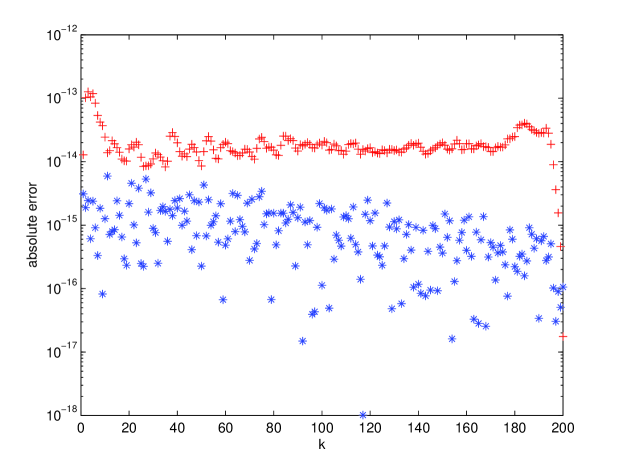
Fig. 3: Forsythe Matrix. Lower (blue) curve: Absolute errors $|c_{k}^{alg2}(F)-c_{k}(F)|$ of the coefficients computed by Algorithm 2. Upper (red) curve: Running error bounds $\rho_{k}$ from Corollary 9.

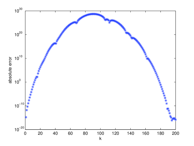
Fig. 4: Forsythe Matrix. Coefficients $c_{k}^{poly}(F)$ computed by poly. The exact coefficients are $c_{k}=0$, $1\leq k\leq 199$.

7.1 The Forsythe Matrix

This example illustrates that Algorithm 2 can compute the coefficients of a highly nonsymmetric matrix more accurately than poly, and that the running error bounds from Corollary 9 approximate the roundoff error from Algorithm 2 well.

We choose a $n\times n$ Forsythe matrix, which is a perturbed Jordan block of the form

$$F_{2}=\begin{pmatrix}0&1&&&\\ &\ddots&\ddots&&\\ &&0&1&\\ \nu&&&0&\end{pmatrix},\qquad\mathrm{where}\quad\nu=10^{-10},$$ (8)

with characteristic polynomial $p(\lambda)=\lambda^{n}-\nu$. Then we perform an orthogonal similarity transformation $F_{1}=QF_{2}Q^{T}$, where $Q$ is an orthogonal matrix obtained from the QR decomposition of a random matrix. The orthogonal similarity transformation to upper Hessenberg form $F$ is produced by $F=$ hess$(F_{1})$.

We applied Algorithm 2 to a matrix $F$ of order $n=200$. Figure 3 shows that Algorithm 2 produces absolute errors of about $10^{-15}$, and that the running error bounds from Corollary 9 approximate the roundoff error from Algorithm 2 well. In contrast, the absolute errors produced by poly are huge, as Figure 4 shows.

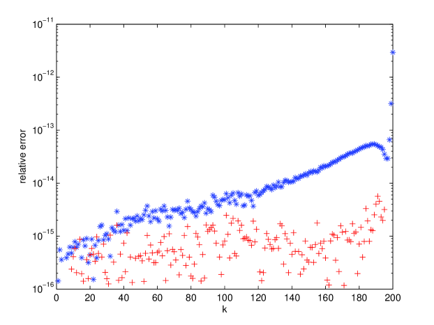
Fig. 5: Hansen’s Matrix. Upper (blue) curve: Relative errors $|c_{k}^{poly}(H)-c_{k}(H)|/|c_{k}(H)|$ of coefficients computed by poly. Lower (red) curve: Relative errors $|c_{k}^{alg1}(H)-c_{k}(H)|/|c_{k}(H)|$ of coefficients computed by Algorithm 1.

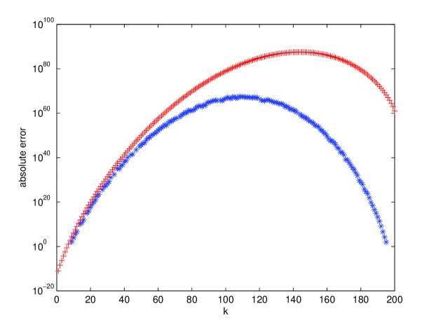
Fig. 6: Hansen’s Matrix. Lower (blue) curve: Absolute errors $|c_{k}^{alg1}(H)-c_{k}|$ in the coefficients computed by Algorithm 1. Upper (red) curve: Running error bounds $\phi_{k}$ from Corollary 5.

7.2 Hansen’s Matrix

This example illustrates that Algorithm 1 can compute the characteristic polynomial of a symmetric positive definite matrix to machine precision.

Hansen’s matrix [12, p 107] is a rank one perturbation of a $n\times n$ symmetric tridiagonal Toeplitz matrix,

$$H=\begin{pmatrix}1&-1&&\\ -1&2&\ddots&\\ &\ddots&\ddots&-1\\ &&-1&2\end{pmatrix}.$$

Hansen’s matrix is positive definite, and the coefficients of its characteristic polynomial are

$$c_{n-k+1}(H)=(-1)^{n-k+1}{n+k-1\choose n-k+1},\qquad 1\leq k\leq n.$$

Figure 5 illustrates for $n=200$ that the Algorithm 1 computes the coefficients to machine precision, and that later coefficients have higher relative accuracy than those computed by poly. With regard to absolute errors, Figure 6 indicates that the running error bounds $\phi_{j}$ from Corollary 5 reflect the trend of the errors, but the bounds become more and more pessimistic for larger $k$.

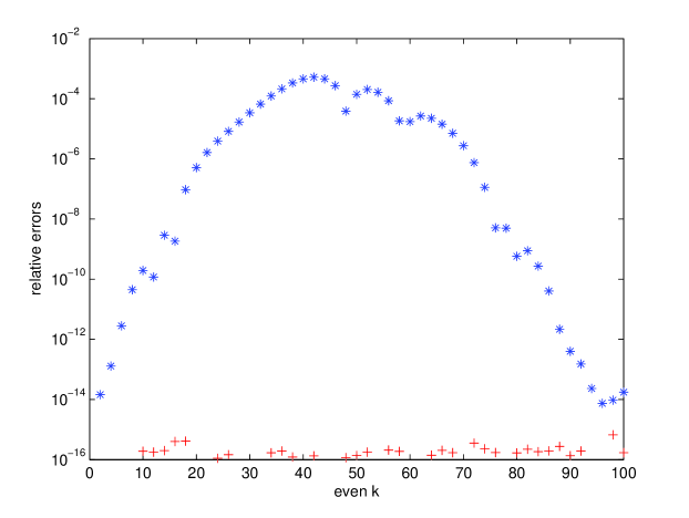
Fig. 7: Symmetric Indefinite Tridiagonal Toeplitz Matrix. Upper (blue) curve: Relative errors $|c_{k}^{poly}(T)-c_{k}(T)|/|c_{k}(T)|$ in the coefficients computed by poly for even $k$. Lower (red) curve: Relative errors $|c_{k}^{alg1}(T)-c_{k}(T)|/|c_{k}(T)|$ in the coefficients computed by Algorithm 1 for even $k$.

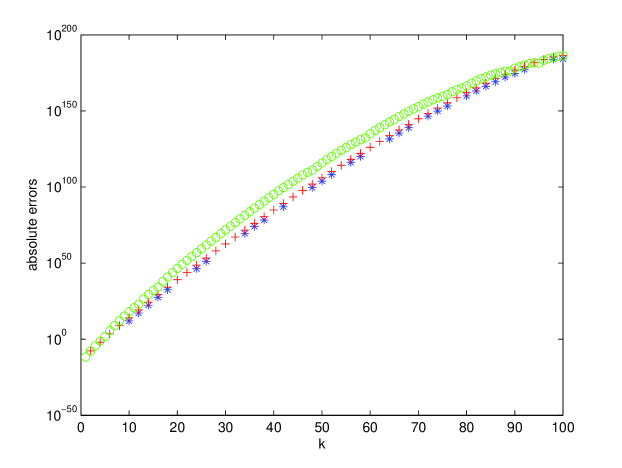
Fig. 8: Symmetric Indefinite Tridiagonal Toeplitz Matrix. Lower (blue) curve: Absolute errors $|c_{k}^{alg1}(T)-c_{k}(T)|$ in the coefficients computed by Algorithm 1. Middle (red) curve: Running error bounds $\phi_{j}$ from Corollary 5. Upper (green) curve: Absolute errors $|c_{k}^{poly}(T)-c_{k}(T)|$ in the coefficients computed by poly.

7.3 Symmetric Indefinite Toeplitz Matrix

This example illustrates that Algorithm 1 can compute the characteristic polynomial of a symmetric indefinite matrix to high relative accuracy, and that the running error bounds in Corollary 5 capture the absolute error well.

The matrix is a $n\times n$ symmetric indefinite tridiagonal Toeplitz matrix

$$T=\begin{pmatrix}0&100&&\\ 100&\ddots&\ddots&&\\ &\ddots&0&100\\ &&100&0\end{pmatrix},$$

where the coefficients with index are zero, i.e. $c_{2j-1}(T)=0$ for $j\geq 1$.

For $n=100$ we obtained the exact coefficients $c_{k}(T)$ with sym2poly(poly(sym(T))) from MATLAB’s symbolic toolbox. Algorithm 1 computes the coefficients with odd index exactly, i.e. $c_{2j-1}^{(i)}(T)=0$ for $j\geq 1$ and $1\leq i\leq n$. In contrast, as Figure 8 shows, the coefficients computed by poly can have magnitudes as large $10^{185}$.

Figure 7 illustrates that Algorithm 1 computes the coefficients $c_{2j}(T)$ with even index to machine precision, while the coefficients computed with poly have relative errors that are many magnitudes larger. Figure 8 also shows that the running error bounds approximate the true absolute error very well. What is not visible in Figure 8, but what one can show from Theorems 2 and 3 is that $\phi_{2j-1}=0$. Hence the running error bounds recognize that $c_{2j-1}$ are computed exactly.

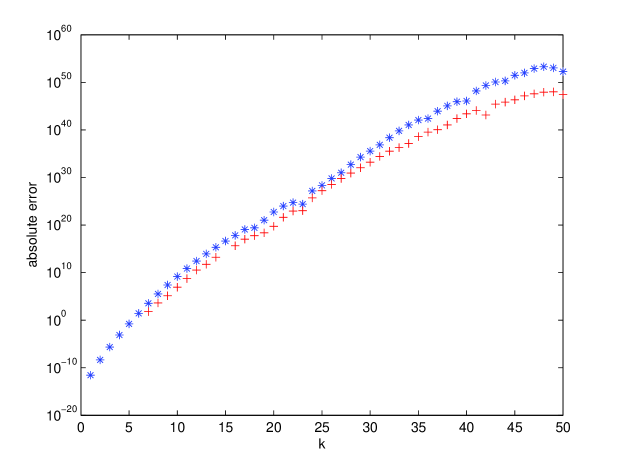
Fig. 9: Frank Matrix. Upper (blue) curve: Absolute errors $|c_{k}^{poly}(U)-c_{k}(U)|$ in the coefficients computed by poly. Lower (red) curve: Absolute errors $|c_{k}^{alg2}(U)-c_{k}(U)|$ in the coefficients computed by Algorithm 2.

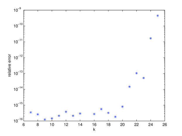
Fig. 10: Frank Matrix. Relative errors $|c_{k}^{alg2}(U)-c_{k}(U)|/|c_{k}(U)|$ in the first 25 coefficients computed by Algorithm 2.

7.4 Frank Matrix

This example shows that Algorithm 2 is at least as accurate, if not more accurate than poly for matrices with ill conditioned polynomial coefficients.

The Frank matrix $U$ is an upper Hessenberg matrix with determinant 1 from MATLAB’s gallery command of test matrices. The coefficients of the characteristic polynomial appear in pairs, in the sense that $c_{k}(U)=c_{n-k}(U)$. For a Frank matrix of order $n=50$, we used MATLAB’s toolbox to determine the exact coefficients $c_{k}(U)$ with the command sym2poly(poly(sym(U))). Figure 9 illustrates that Algorithm 2 computes the coefficients at least as accurately as poly. In fact, as seen in Figure 10, Algorithm 2 computes the first 20 coefficients to high relative accuracy.

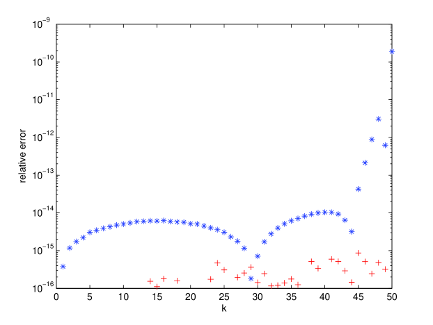
Fig. 11: Transposed Chow Matrix. Upper (blue) curve: Relative errors $|c_{k}^{poly}(C^{T})-c_{k}(C^{T})|/|c_{k}(C^{T})|$ in the coefficients computed by poly. Lower (red) curve: Relative errors $|c_{k}^{alg2}(C^{T})-c_{k}(C^{T})|/|c_{k}(C^{T})|$ in the coefficients computed by Algorithm 2.

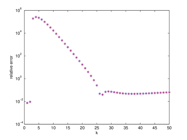
Fig. 12: Chow Matrix. Blue curve: Relative errors $|c_{k}^{poly}(C)-c_{k}(C)|/|c_{k}(C)|$ in the coefficients computed by poly. Red curve: Relative errors $|c_{k}^{alg2}(C)-c_{k}(C)|/|c_{k}(C)|$ in the coefficients computed by Algorithm 2. The two curves are virtually indistinguishable.

7.5 Chow Matrix

This example illustrates that the errors in the reduction to Hessenberg form can be amplified substantially when the coefficients of the characteristic polynomial are illconditioned.

The Chow matrix is a matrix that is Toeplitz as well as lower Hessenberg from MATLAB’s gallery command of test matrices. Our version of the transposed Chow matrix is an upper Hessenberg matrix with powers of 2 in the leading row and trailing column,

$$C^{T}=\begin{pmatrix}3&4&\ldots&2^{n}\\ 1&\ddots&\ddots&\vdots\\ &\ddots&3&4\\ &&1&3\end{pmatrix}.$$

As before, we computed the exact coefficients with MATLAB’s symbolic toolbox. Figure 11 illustrates that Algorithm 2 computes all coefficients $c_{k}(C^{T})$ to high relative accuracy for $n=50$. In contrast, the relative accuracy of the coefficients computed by poly deteriorates markedly as $k$ becomes larger.

However, if we compute instead the characteristic polynomial of $C$, then a preliminary reduction to upper Hessenberg form is necessary. Figure 12 illustrates that the computed coefficients have hardly any relative accuracy to speak of, and only the trailing coefficients have about 1 significant digit. The loss of accuracy occurs because the errors in the reduction to Hessenberg form are amplified by the condition numbers of the coefficients, as the absolute bound in Theorem 11 suggests. Unfortunately, in this case, the condition numbers in Theorem 11 are too pessimistic to predict the absolute error of Algorithm 2.

Acknowledgements

We thank Dean Lee for helpful discussions.

References

[1]S. Barnett, Leverrier’s algorithm: A new proof and extensions, SIAM
J. Matrix Anal. Appl., 10 (1989), pp. 551–556.
[2], Leverrier’s
algorithm for orthogonal bases, Linear Algebra Appl., 236 (1996),
pp. 245–263.
[3]M. D. Bingham, A new method for obtaining the inverse matrix, J.
Amer. Statist. Assoc., 36 (1941), pp. 530–534.
[4]L. Csanky, Fast parallel matrix inversion, SIAM J. Comput., 5
(1976), pp. 618–623.
[5]V. N. Faddeeva, Computational Methods of Linear Algebra, Dover, New
York, 1959.
[6]F. R. Gantmacher, The Theory of Matrices, vol. I, AMS Chelsea
Publishing, Providence, Rhode Island, 1998.
[7]M. Giesbrecht, Nearly optimal algorithms for canonical matrix
forms, SIAM J. Comput., 24 (1995), pp. 948–969.
[8]W. B. Givens, Numerical computation of the characteristic values of
a real symmetric matrix, tech. rep., Oak Ridge National Labortary, 1953.
[9], The characteristic
value-vector problem, J. Assoc. Comput. Mach., 4 (1957),
pp. 298–307.
[10]G. H. Golub and C. F. Van Loan, Matrix Computations, The Johns
Hopkins University Press, Baltimore, third ed., 1996.
[11]S. J. Hammarling, Latent Roots and Latent Vectors, The University
of Toronto Press, 1970.
[12]E. R. Hansen, On the Danilewski method, J. Assoc. Comput. Mach.,
10 (1963), pp. 102–109.
[13]G. Helmberg, P. Wagner, and G. Veltkamp, On Faddeev-Leverrier’s
method for the computation of the characteristic polynomial of a matrix and
of eigenvectors, Linear Algebra Appl., 185 (1993), pp. 219–233.
[14]N. J. Higham, Accuracy and Stability of Numerical Algorithms, SIAM,
Philadelphia, second ed., 2002.
[15]P. Horst, A method for determining the coefficients of the
characteristic equation, Ann. Math. Statistics, 6 (1935), pp. 83–84.
[16]S.-H. Hou, A simple proof of the Leverrier-Faddeev characteristic
polynomial algorithm, SIAM Rev., 40 (1998), pp. 706–709.
[17]A. S. Householder, The Theory of Matrices in Numerical Analysis,
Dover, New York, 1964.
[18]A. S. Householder and F. L. Bauer, On certain methods for expanding
the characteristic polynomial, Numer. Math., 1 (1959), pp. 29–37.
[19]I. Ipsen and R. Rehman, Perturbation bounds for determinants and
characteristic polynomials, SIAM J. Matrix Anal. Appl., 30 (2008),
pp. 762–776.
[20]E. Kaltofen and B. D. Saunders, On Wiedemann’s method of solving
linear systems, in Proc. Ninth Internat. Symp. Applied Algebra, Algebraic
Algor., Error-Correcting Codes, vol. 539 of Lect. Notes Comput. Sci.,
Springer, Berlin, 1991, pp. 29–38.
[21]D. Lee, Private communication.
[22]D. Lee and T. Schaefer, Neutron matter on the lattice with pionless
effective field theory, Phys. Rev. C, 2 (2005), p. 024006.
[23]M. Lewin, On the coefficients of the characteristic polynomial of a
matrix, Discrete Math., 125 (1994), pp. 255–262.
[24]P. Misra, E. Quintana, and P. Van Dooren, Numerically stable
computation of characteristic polynomials, in Proc. American Control
Conference, vol. 6, IEEE, 1995, pp. 4025–4029.
[25]C. Papaconstantinou, Construction of the characteristic polynomial
of a matrix, IEEE Trans. Automatic Control., 19 (1974), pp. 149–151.
[26]R. Rehman, Numerical Computation of the Characteristic Polynomial of
a Complex Matrix, PhD thesis, Department of Mathematics, North Carolina
State University, 2010.
[27]R. Rehman and I. Ipsen, Computing characteristic polynomials from
eigenvalues, SIAM J. Matrix Anal. Appl.
In revision.
[28]P. A. Samuelson, A method of determining explicitly the coefficients
of the characteristic equation, Ann. Math. Statistics, 13 (1942),
pp. 424–429.
[29]J. Wang and C.-T. Chen, On the computation of the characteristic
polynomial of a matrix, IEEE Trans. Automatic Control., 27 (1982),
pp. 449–451.
[30]D. H. Wiedemann, Solving sparse linear equations over finite
fields, IEEE Trans. Inf. Theory, IT-32 (1986), pp. 54–62.
[31]J. Wilkinson, The Algebraic Eigenvalue Problem, Oxford University
Press, 1965.
[32]J. H. Wilkinson, The perfidious polynomial, in Studies in Numerical
Analysis, G. H. Golub, ed., vol. 24 of MAA Stud. Math., Math. Assoc. America,
Washington, DC, 1984, pp. 1–28.