Finite amplitude method for the quasi-particle-random-phase approximation

Abstract

We present the finite amplitude method (FAM), originally proposed in Ref. fam , for superfluid systems. A Hartree-Fock-Bogoliubov code may be transformed into a code of the quasi-particle-random-phase approximation (QRPA) with simple modifications. This technique has advantages over the conventional QRPA calculations, such as coding feasibility and computational cost. We perform the fully self-consistent linear-response calculation for a spherical neutron-rich nucleus ¹⁷⁴Sn, modifying the HFBRAD code, to demonstrate the accuracy, feasibility, and usefulness of the FAM.

I Introduction

Elementary modes of excitation in nuclei provide valuable information about the nuclear structure. The random-phase approximation (RPA) based on energy density functionals (EDF) is a leading theory applicable both to low-lying excited states and giant resonances RS ; Bender . Although the fully self-consistent treatment of the residual (induced) interactions for the realistic energy functionals is becoming more and more prevalent Imagawa ; Paar ; Nakatsukasa ; Terasaki1 ; Fracasso ; Sil ; Terasaki2 ; Artega ; Peru ; Losa ; Terasaki-def , the RPA calculations for deformed nuclei are still computationally demanding. At present, the quasi-particle random-phase approximation (QRPA) for deformed superfluid nuclei are limited only to axially deformed cases Artega ; Peru ; Yoshi1 ; Losa ; Terasaki-def ; Yoshi2 , except for Ref. Ebata with an approximate treatment of the pairing interaction.

Recently, there has been a renewed interest in the solution of the RPA problem fam ; Inakura ; DobaArnoldi . In Ref. fam , the finite amplitude method (FAM) was proposed as a feasible method for a solution of the RPA equation. The FAM allows to calculate all the induced fields as a finite difference, employing a computational program of the static mean-field Hamiltonian. Recently, the FAM has been applied to the electric dipole excitations in nuclei using the Skyrme energy functionals Inakura . There has been also a calculation making use the iterative Arnoldi algorithm for a solution of the RPA equation DobaArnoldi . These newly developed technologies in conjunction with fast solving algorithms for linear systems open the possibility to explore systematically the nuclear excitations over the entire nuclear chart.

So far, these new techniques fam ; Inakura ; DobaArnoldi have been developed for solutions of the RPA without the pairing correlations. It is well known, however, that almost all but magic nuclei display superfluid features. Therefore, a further improvement is highly desirable to make these methods applicable to the QRPA equations including correlations in the particle-particle and hole-hole channels. The purpose of the present paper is to generalize the FAM to superfluid systems, which enables us to perform a QRPA calculation utilizing a static Hartree-Fock-Bogoliubov (HFB) code with minor modifications. Our final goal would be the construction of a fast computer program for the fully self-consistent and triaxially deformed QRPA. This paper is a first step toward the goal, to present the basic equations of the FAM for the QRPA and show the first result for spherical nuclei. We use the spherically symmetric HFB code called HFBRAD BennaDoba to be converted into the QRPA code.

This paper is organized as follows: In Sec. II, the QRPA equation is derived as the small-amplitude limit of the time-dependent HFB (TDHFB) equations. In Sec. III, we obtain the FAM formulae for the calculation of the induced fields. In Sec. IV, we summarize all the relevant formulae for practical application of the FAM. In Sec. V, we apply the FAM to the HFBRAD and compare the result with that of another self-consistent calculation. Sec. VI is devoted to the conclusions.

II Small amplitude limit of the TDHFB

In this section, we recapitulate the basic formulation of the TDHFB and its small-amplitude limit. In general, we will follow the notation in Ref. RS unless otherwise specified. We also use $\hbar=1$ in the following equations.

We start from the energy functional $\mathcal{E}[\rho,\kappa,\kappa^{*}]$ which is a functional of the density matrix and pairing tensor.

$$\begin{split}\rho_{kl}=\langle\Phi|c^{\dagger}_{l}c_{k}|\Phi\rangle,~{}~{}~{}\kappa_{kl}=\langle\Phi|c_{l}c_{k}|\Phi\rangle,\end{split}$$ (1)

where $|\Phi\rangle$ is the HFB state. The single-particle Hamiltonian $h$ and the pairing potential $\Delta$ are obtained with a variation of the energy functional with respect to $\rho$ and $\kappa^{*}$, respectively.

$$\begin{split}h_{kl}[\rho,\kappa,\kappa^{*}]=\frac{\partial\mathcal{E}}{\partial\rho_{lk}},~{}~{}~{}\Delta_{kl}[\rho,\kappa,\kappa^{*}]=\frac{\partial\mathcal{E}}{\partial\kappa^{*}_{kl}}.\end{split}$$ (2)

The Bogoliubov quasi-particles, $(a_{\mu},a_{\mu}^{\dagger})$, have a linear connection to the bare particles, $(c_{k},c_{k}^{\dagger})$; $a_{\mu}^{\dagger}=\sum_{k}(U_{k\mu}c_{k}^{\dagger}+V_{k\mu}c_{k})$. Here, the index $k$ indicates the adopted basis such as the harmonic oscillator states or the coordinate space. The quasi-particles $a_{\mu}$ are chosen so as to diagonalize the HFB Hamiltonian RS .

$$H_{0}=\frac{1}{2}\begin{pmatrix}c^{\dagger}&c\end{pmatrix}\begin{pmatrix}h-\lambda&\Delta\\ -\Delta^{*}&-(h^{*}-\lambda)\end{pmatrix}\begin{pmatrix}c\\ c^{\dagger}\end{pmatrix}=\sum_{\mu}E_{\mu}a_{\mu}^{\dagger}a_{\mu}.$$ (3)

Here, the normal ordering is assumed.

In a similar manner, the time-dependent quasi-particles $a_{\mu}^{\dagger}(t)$ are characterized by the time-dependent wave functions $(U(t),V(t))$ by $a_{\mu}^{\dagger}(t)=\sum_{k}\{U_{k\mu}(t)c_{k}^{\dagger}+V_{k\mu}(t)c_{k}\}$. The time evolution of the quasi-particles under a one-body external perturbation $F(t)$ are determined by the following TDHFB equation.

$$i\frac{\partial a_{\mu}(t)}{\partial t}=[H(t)+F(t),a_{\mu}(t)],$$ (4)

where the TDHFB Hamiltonian is given by

$$H(t) = \sum_{kl}\left\{h_{kl}(t)-\lambda\delta_{kl}\right\}c_{k}^{\dagger}c_{l}$$ (5)

$$+\sum_{k>l}\left\{\Delta_{kl}(t)c_{k}^{\dagger}c_{l}^{\dagger}+\Delta_{kl}^{*}(t)c_{l}c_{k}\right\}$$

$$= \frac{1}{2}\begin{pmatrix}c^{\dagger}&c\end{pmatrix}\begin{pmatrix}h(t)-\lambda&\Delta(t)\\ \Delta^{\dagger}(t)&-(h^{*}(t)-\lambda)\end{pmatrix}\begin{pmatrix}c\\ c^{\dagger}\end{pmatrix}$$

Here and hereafter, the constant shift is neglected, since it does not play any role in the TDHFB equation (4). $h(t)$ and $\Delta(t)$ become time-dependent, since they depend on the densities, $\rho(t)=V^{*}(t)V^{T}(t)$ and $\kappa(t)=V^{*}(t)U^{T}(t)=-U(t)V^{\dagger}(t)$, which are time-dependent. Note that the static quasi-particles correspond to a quasi-static solution of Eq. (4), $a_{\mu}(t)=a_{\mu}e^{iE_{\mu}t}$, with $F(t)=0$.

Let us assume that the nucleus is under a weak external field of a given frequency $\omega$.

$$F(t) = \eta\left\{F(\omega)e^{-i\omega t}+F^{\dagger}(\omega)e^{i\omega t}\right\},$$ (6)

$$F(\omega) = \frac{1}{2}\sum_{\mu\nu}\left\{F_{\mu\nu}^{20}(\omega)A_{\mu\nu}^{\dagger}+F_{\mu\nu}^{02}(\omega)A_{\mu\nu}\right\}$$ (7)

$$+\sum_{\mu\nu}F_{\mu\nu}^{11}(\omega)B_{\mu\nu},$$

where $A_{\mu\nu}^{\dagger}\equiv a_{\mu}^{\dagger}a_{\nu}^{\dagger}$ and $B_{\mu\nu}\equiv a_{\mu}^{\dagger}a_{\nu}$. A small real parameter $\eta$ is introduced for the linearization. In the small-amplitude limit, the second term ($B$-part) in Eq. (7) can be omitted, because it doesn’t contribute in the linear approximation. The Bogoliubov transformation of the external fields ($F_{\mu\nu}^{20}(\omega)$ and $F_{\mu\nu}^{02}(\omega)$) is given in Appendix A.2.

The external perturbation $F(t)$ induces a density oscillation around the ground state with the same frequency $\omega$. The density oscillation, then, produces the induced fields in the single-particle Hamiltonian, $h(t)=h_{0}+\delta h(t)$ and in the pair potential, $\Delta(t)=\Delta+\delta\Delta(t)$. Thus, the Hamiltonian, Eq. (5), is decomposed into the static and oscillating parts; $H(t)=H_{0}+\delta H(t)$.

$$\delta H(t) = \eta\left\{\delta H(\omega)e^{-i\omega t}+\delta H^{\dagger}(\omega)e^{i\omega t}\right\},$$ (8)

$$\delta H(\omega) = \frac{1}{2}\sum_{\mu\nu}\left\{\delta H_{\mu\nu}^{20}(\omega)A_{\mu\nu}^{\dagger}+\delta H_{\mu\nu}^{02}(\omega)A_{\mu\nu}\right\}.$$ (9)

Here, the $B$-part is again neglected in Eq. (9). See Appendix A.1 for the derivation of $\delta H(\omega)$. Explicit expressions for $\delta H_{\mu\nu}^{20}(\omega)$ and $\delta H_{\mu\nu}^{02}(\omega)$ are found in Eqs. (50) and (51), respectively.

The time-dependent quasi-particle operators are decomposed in a similar manner:

$$a_{\mu}(t)=\{a_{\mu}+\delta a_{\mu}(t)\}e^{iE_{\mu}t},$$ (10)

where $\delta a_{\mu}(t)$ can be expanded in the quasi-particle creation operators:

$$\delta a_{\mu}(t)=\eta\sum_{\nu}a^{\dagger}_{\nu}\left(\frac{}{}X_{\nu\mu}(\omega)e^{-i\omega t}+Y_{\nu\mu}^{*}(\omega)e^{i\omega t}\right)\ .$$ (11)

It should be noted that $\delta a_{\mu}$ can be expanded only in terms of the creation operators, because the annihilation operators in the right-hand side of Eq. (11) simply represent the transformation among themselves, $a_{\mu}(t)=\sum_{\nu}C_{\mu\nu}(t)a_{\nu}$, and do not affect $\rho$ and $\kappa$. The amplitudes, $X$ and $Y$, must be anti-symmetric to satisfy the fermionic commutation relation, $\{a_{\mu}(t),a_{\nu}(t)\}=0$. Keeping only linear terms in $\eta$, Eq. (4) becomes

$$i\frac{\partial\delta a_{\mu}(t)}{\partial t}=E_{\mu}\delta a_{\mu}(t)+[H_{0},\delta a_{\mu}(t)]+[\delta H(t)+F(t),a_{\mu}].$$ (12)

Substituting Eqs. (6)-(11) into Eq. (12), we obtain the linear-response equations:

$$\left\{\begin{array}[]{cc}\displaystyle\left(E_{\mu}+E_{\nu}-\omega\right)X_{\mu\nu}(\omega)+\delta H^{20}_{\mu\nu}(\omega)&=F^{20}_{\mu\nu}(\omega)\\ \displaystyle\left(E_{\mu}+E_{\nu}+\omega\right)Y_{\mu\nu}(\omega)+\delta H^{02}_{\mu\nu}(\omega)&=F^{02}_{\mu\nu}(\omega)\end{array}\right..$$ (13)

In Eq. (13), setting the frequency complex, $\omega\rightarrow\omega+i\gamma/2$, we can introduce a smearing with a width $\gamma$.

Expanding $\delta H^{20}(\omega)$ and $\delta H^{02}(\omega)$ in terms of the forward and backward amplitudes, $X$ and $Y$, we obtain a familiar expression of the equation RS :

$$\left[\!\left(\begin{array}[]{cc}A&B\\ B^{*}&A^{*}\end{array}\right)-\omega\left(\begin{array}[]{cc}I\!\!I&~{}~{}0\\ 0&-I\!\!I\end{array}\right)\right]\left(\begin{array}[]{c}X(\omega)\\ Y(\omega)\end{array}\right)\!=\!\left(\!\begin{array}[]{c}F^{20}(\omega)\\ F^{02}(\omega)\end{array}\!\right).$$ (14)

This matrix formulation requires us to calculate the QRPA matrix elements, $A_{\mu\nu,\mu^{\prime}\nu^{\prime}}$ and $B_{\mu\nu,\mu^{\prime}\nu^{\prime}}$. This is a tedious task and their dimension, which is equal to the number of two-quasi-particle excitations, becomes huge especially for deformed nuclei. Instead, in the FAM fam , we keep the form of Eq. (13) and calculate the induced fields $\delta H^{20}(\omega)$ and $\delta H^{02}(\omega)$ using the numerical differentiation. We explain this trick in the next section.

III Finite amplitude method for the induced fields

The expressions for $\delta H^{20}$ and $\delta H^{02}$ in Eq. (13) are given in Eqs. (50) and (51), respectively. Thus, we need to calculate $\delta h(\omega)$ and $\delta\Delta^{(\pm)}(\omega)$ for given $X$ and $Y$. We perform this calculation following the spirit of the FAM fam .

From Eqs. (10) and (11), we obtain the time-dependent quasi-particle wave functions:

$$\begin{pmatrix}U_{\mu}(t)\\ V_{\mu}(t)\end{pmatrix}=\begin{pmatrix}\mathcal{U}_{\mu}(t)\\ \mathcal{V}_{\mu}(t)\end{pmatrix}e^{iE_{\mu}t},$$ (15)

where

$$\mathcal{U}_{k\mu}(t) = \left\{U+\eta\left(V^{*}X^{*}e^{i\omega t}+V^{*}Ye^{-i\omega t}\right)\right\}_{k\mu},\ \$$ (16)

$$\mathcal{V}_{k\mu}(t) = \left\{V+\eta\left(U^{*}X^{*}e^{i\omega t}+U^{*}Ye^{-i\omega t}\right)\right\}_{k\mu}.\ \$$ (17)

First, let us discuss how to obtain $\delta h(\omega)$. The time-dependent single-particle Hamiltonian $h(t)$ depends on the densities which are determined by the wave functions $(U(t),V(t))$. Therefore, $h(t)$ can be regarded as a functional of wave functions as

$$h\left[U^{*}(t),V^{*}(t);U(t),V(t)\right]=h\left[\mathcal{U}^{*}(t),\mathcal{V}^{*}(t);\mathcal{U}(t),\mathcal{V}(t)\right].$$ (18)

Here, it should be noted that the phase factors, $e^{iE_{\mu}t}$ in Eq. (15), do not play a role. This is because $h$ is a functional of densities, $\rho$, $\kappa$, and $\kappa^{*}$, which are given by products of one of $(U,V)$ and one of the complex conjugate $(U^{*},V^{*})$, such as $\rho=V^{*}V^{T}$ and $\kappa=V^{*}U^{T}$. Therefore, the time-dependent phases in Eq. (15) are always canceled, thus can be omitted.

Now, we take the small-amplitude limit, keeping only the linear order in $\eta$.

$$h(t) = h\left[\mathcal{U}^{*}(t),\mathcal{V}^{*}(t);\mathcal{U}(t),\mathcal{V}(t)\right]$$ (19)

$$= h\left[U^{*},V^{*};U,V\right]+\eta\left\{\delta h(\omega)e^{-i\omega t}+\mbox{h.c.}\right\}.$$

Here, $\delta h(\omega)$ can be obtained using Eqs. (16) and (17), expanding up to the first order in $\eta$ and collecting terms proportional to $e^{-i\omega t}$, as

$$\delta h(\omega) = \frac{\partial h}{\partial U^{*}}\cdot VX+\frac{\partial h}{\partial V^{*}}\cdot UX$$ (20)

$$+\frac{\partial h}{\partial U}\cdot V^{*}Y+\frac{\partial h}{\partial V}\cdot U^{*}Y.$$

The calculation of the derivatives, such as $\partial h_{kl}/\partial U^{*}_{k^{\prime}\mu}$, is a tedious task and requires a large memory capacity for their storage in the computation. In the FAM, we avoid this explicit expansion, instead write the same quantity as follows:

$$\delta h(\omega)=\frac{h\left[\bar{U}_{\eta}^{*},\bar{V}_{\eta}^{*};U_{\eta},V_{\eta}\right]-h\left[U^{*},V^{*};U,V\right]}{\eta}+\mathcal{O}(\eta^{2}),$$ (21)

where $\bar{U}_{\eta}^{*}$, $\bar{V}_{\eta}^{*}$, $U_{\eta}$, and $V_{\eta}$ are given by

$$\begin{split}\bar{U}_{\eta}^{*}&\equiv U^{*}+\eta VX,\quad\bar{V}_{\eta}^{*}\equiv V^{*}+\eta UX,\\ U_{\eta}&\equiv U+\eta V^{*}Y,\quad V_{\eta}\equiv V+\eta U^{*}Y.\end{split}$$ (22)

This is the FAM formula for the calculation of $\delta h(\omega)$. All we need in the computer program is a subroutine to calculate the single-particle Hamiltonian as a function of the wave functions, $h[\bar{U}^{*},\bar{V}^{*};U,V]$.

For the pair potential, basically, the same arguments lead to the FAM formulae for $\delta\Delta^{(\pm)}$. The time-dependent pair potential $\Delta(t)$ can be written as

$$\Delta(t) = \Delta\left[\mathcal{U}^{*}(t),\mathcal{V}^{*}(t);\mathcal{U}(t),\mathcal{V}(t)\right]$$ (23)

$$= \Delta\left[U^{*},V^{*};U,V\right]$$

$$+\eta\left\{\delta\Delta^{(+)}(\omega)e^{-i\omega t}+\delta\Delta^{(-)}(\omega)e^{i\omega t}\right\}.$$

Here, $\delta\Delta^{(+)}$ and $\delta\Delta^{(-)}$ are independent, since $\Delta(t)$ is non-Hermitian in general. $\delta\Delta^{(+)}$ can be written in the same form as Eq. (21).

$$\delta\Delta^{(+)}(\omega) = \frac{\Delta\left[\bar{U}_{\eta}^{*},\bar{V}_{\eta}^{*};U_{\eta},V_{\eta}\right]-\Delta\left[U^{*},V^{*};U,V\right]}{\eta}$$ (24)

$$+\mathcal{O}(\eta^{2}),$$

where $\bar{U}_{\eta}^{*}$, $\bar{V}_{\eta}^{*}$, $U_{\eta}$, and $V_{\eta}$ are given by Eq. (22).

The expression for $\delta\Delta^{(-)}$ is also obtained from Eq. (23), collecting terms proportional to $e^{i\omega t}$. It is given by the same expression as Eq. (24),

$$\delta\Delta^{(-)}(\omega) = \frac{\Delta\left[\bar{U}_{\eta}^{*},\bar{V}_{\eta}^{*};U_{\eta},V_{\eta}\right]-\Delta\left[U^{*},V^{*};U,V\right]}{\eta}$$ (25)

$$+\mathcal{O}(\eta^{2}).$$

However, $(\bar{U}_{\eta}^{*},\bar{V}_{\eta}^{*};U_{\eta},V_{\eta})$ here are different from Eq. (22) and given by

$$\begin{split}\bar{U}_{\eta}^{*}&\equiv U^{*}+\eta VY^{*},\quad\bar{V}_{\eta}^{*}\equiv V^{*}+\eta UY^{*},\\ U_{\eta}&\equiv U+\eta V^{*}X^{*},\quad V_{\eta}\equiv V+\eta U^{*}X^{*}.\end{split}$$ (26)

The essential trick of the FAM is to calculate the induced fields, $\delta h(\omega)$ and $\delta\Delta^{(\pm)}$, according to Eqs. (21), (24), and (25) with a small but finite parameter $\eta$. Of course, the $\eta^{2}$ and higher-order terms bring some numerical errors, but they are negligible. Therefore, for given $X$ and $Y$, we are able to calculate these induced fields, by using the static HFB code with some minor modifications. $\delta H^{20}(\omega)$ and $\delta H^{02}(\omega)$ of Eq. (13) in the quasi-particle basis can be calculated with Eqs. (50) and (51), respectively. Then, we may solve the QRPA linear-response equation (13) to obtain the self-consistent amplitudes, $X$ and $Y$, utilizing an iterative algorithm (See Sec. IV).

III.1 Induced fields in terms of densities

Although the basic formulae of the FAM has been provided in Sec. III, we may need to modify them in the practical implementation of the FAM. For instance, some HFB codes, such as HFBRAD, contain subroutines to calculate mean fields as functions of densities, not of wave functions. In this subsection, we rewrite Eqs. (21), (24), and (25) in terms of densities.

The density $\delta\rho(t)$ is written up to linear order in $\eta$ as

$$\begin{split}\rho(t)&=V^{*}(t)V^{T}(t)\\ &=\rho_{0}+\eta\left(\delta\rho(\omega)e^{-i\omega t}+\mbox{h.c.}\right),\end{split}$$ (27)

where

$$\delta\rho(\omega)=UXV^{T}+V^{*}Y^{T}U^{\dagger}.$$ (28)

This can be written in the FAM form:

$$\delta\rho(\omega) = \frac{\rho_{\eta}-\rho_{0}}{\eta}+\mathcal{O}(\eta^{2})$$ (29)

$$= \frac{\bar{V}_{\eta}^{*}V_{\eta}^{T}-V^{*}V^{T}}{\eta}+\mathcal{O}(\eta^{2}),$$

where $\bar{V}_{\eta}^{*}$ and $V_{\eta}$ are given in Eq. (22).

The pair tensor $\kappa(t)$, which is non-Hermitian, can be expressed in a similar manner.

$$\begin{split}\kappa(t)&=V^{*}(t)U^{T}(t)\\ &=\kappa_{0}+\eta\left(\delta\kappa^{(+)}e^{-i\omega t}+\delta\kappa^{(-)}e^{i\omega t}\right).\end{split}$$ (30)

Here, $\kappa^{(\pm)}$ can be given in the explicit form as

$$\delta\kappa^{(+)}(\omega) =UXU^{T}+V^{*}Y^{T}V^{\dagger},$$ (31)

$$\delta\kappa^{(-)}(\omega) =V^{*}X^{\dagger}V^{\dagger}+UY^{*}U^{T},$$ (32)

and in the FAM form as

$$\delta\kappa^{(\pm)}(\omega) = \frac{\kappa_{\eta}^{(\pm)}-\kappa_{0}}{\eta}+\mathcal{O}(\eta^{2})$$ (33)

$$= \frac{\bar{V}_{\eta}^{*}U_{\eta}^{T}-V^{*}U^{T}}{\eta}+\mathcal{O}(\eta^{2}),$$

where $\bar{V}_{\eta}^{*}$ and $U_{\eta}$ are given in Eq. (22) for $\kappa_{\eta}^{(+)}$ while they are given by Eq. (26) for $\kappa_{\eta}^{(-)}$.

Now, let us present how to obtain the induced fields in terms of the densities. In general, $h(t)$ and $\Delta(t)$ may depend on $\rho$, $\kappa$, and $\kappa^{*}$.

$$h(t)=h\left[\rho(t),\kappa(t),\kappa^{*}(t)\right],\quad\Delta(t)=\Delta\left[\rho(t),\kappa(t),\kappa^{*}(t)\right].$$ (34)

In order to obtain the induced fields, all we need to do is to replace $\rho$ by $\rho_{\eta}$ defined in Eqs. (29), and $\kappa$ by $\kappa_{\eta}^{(\pm)}$ in Eq. (33), as follows:

$$\delta h(\omega) = \frac{h\left[\rho_{\eta},\kappa_{\eta}^{(+)},\kappa_{\eta}^{(-)*}\right]-h\left[\rho,\kappa,\kappa^{*}\right]}{\eta},$$ (35)

$$\delta\Delta^{(+)}(\omega) = \frac{\Delta\left[\rho_{\eta},\kappa_{\eta}^{(+)},\kappa_{\eta}^{(-)*}\right]-\Delta\left[\rho,\kappa,\kappa^{*}\right]}{\eta},$$ (36)

$$\delta\Delta^{(-)}(\omega) = \frac{\Delta\left[\rho_{\eta},\kappa_{\eta}^{(-)},\kappa_{\eta}^{(+)*}\right]-\Delta\left[\rho,\kappa,\kappa^{*}\right]}{\eta},$$ (37)

where the terms of the second and higher orders in $\eta$ are neglected.

IV Summary of The Finite Amplitude Method

Here we provide a summary of the FAM for the QRPA linear-response calculation for a prompt application. Later, we discuss applications of the FAM to the Skyrme functionals, however, the FAM formulated in this and previous sections is applicable to any kind of energy density functional (mean-field) models.

IV.1 Numerical procedure

The aim is to solve the linear-response equation (13) for a given external field $F$. In order to obtain the forward and backward amplitudes, $X$ and $Y$, we resort to an iterative algorithm. Namely, we start from the initial guess for $(X,Y)=(X^{(0)},Y^{(0)})\equiv\vec{x}^{(0)}$, and calculate $\delta h(\omega)$ and $\delta\Delta^{(\pm)}(\omega)$ according to the formulae, (21), (24), and (25). Then, they are converted into $\delta H^{20}(\omega)$ and $\delta H^{02}(\omega)$, using Eqs. (50) and (51), respectively. In this way, we can evaluate the left and right hand sides of Eq. (13) for a given $(X,Y)$.

Since Eq. (13) is equivalent to Eq. (14), it is a linear algebraic equation for the vector $\vec{x}\equiv(X,Y)$, in the form of $A\vec{x}=\vec{b}$. Many different algorithms are available for the solution of linear systems. In this paper, we resort to a procedure based on Krylov spaces called generalized conjugate residual (GCR) method Saad . Within these kinds of methods, a succession of approximate solutions ($\vec{x}^{(0)},\vec{x}^{(1)},\vec{x}^{(2)},\cdots$) converging to the exact one is obtained by the iteration. The GCR algorithm consists in a series of steps each containing the operation of the matrix $A$ on a given vector, and sums and scalar products of two vectors. For the given $\vec{x}=(X,Y)$, $A\vec{x}$ is equal to the left hand side of Eq. (13). Therefore, the quantity $A\vec{x}$ can be calculated without the explicit knowledge of the QRPA matrix itself.

Here, we summarize the formulae. The linear response equation is given by $A\vec{x}=\vec{b}$, where

$$\vec{x}\equiv\begin{pmatrix}X_{\mu\nu}\\ Y_{\mu\nu}\end{pmatrix},\quad\vec{b}\equiv\begin{pmatrix}F_{\mu\nu}^{20}\\ F_{\mu\nu}^{02}\end{pmatrix},$$

and

$$A\vec{x}=\begin{pmatrix}\left(E_{\mu}+E_{\nu}-\omega\right)X_{\mu\nu}(\omega)+\delta H^{20}_{\mu\nu}(\omega)\\ \left(E_{\mu}+E_{\nu}+\omega\right)Y_{\mu\nu}(\omega)+\delta H^{02}_{\mu\nu}(\omega)\end{pmatrix},$$

where

$$\delta H^{20}_{\mu\nu}(\omega) = U^{\dagger}\delta hV^{*}-V^{\dagger}\delta\Delta^{(-)*}V^{*}$$

$$+ U^{\dagger}\delta\Delta^{(+)}U^{*}-V^{\dagger}\delta h^{T}U^{*},$$

$$\delta H^{02}_{\mu\nu}(\omega) = -V^{T}\delta hU+U^{T}\delta\Delta^{(-)*}U$$

$$- V^{T}\delta\Delta^{(+)}V+U^{T}\delta h^{T}V.$$

Denoting $h$ and $\Delta$ collectively as $\mathcal{H}\equiv(h,\Delta)$, the induced fields $\delta\mathcal{H}$ are calculated by the FAM formulae,

$$\delta\mathcal{H}=\frac{\mathcal{H}\left[\bar{U}_{\eta}^{*},\bar{V}_{\eta}^{*};U_{\eta},V_{\eta}\right]-\mathcal{H}\left[U^{*},V^{*};U,V\right]}{\eta},\\$$ (38)

where $(\bar{U}_{\eta}^{*},\bar{V}_{\eta}^{*};U_{\eta},V_{\eta})$ are given by

$$\bar{U}_{\eta}^{*} \equiv U^{*}+\eta VY^{*},\quad\bar{V}_{\eta}^{*}\equiv V^{*}+\eta UY^{*},$$

$$U_{\eta} \equiv U+\eta V^{*}X^{*},\quad V_{\eta}\equiv V+\eta U^{*}X^{*}.$$

for the calculation of $\delta h(\omega)$ and $\delta\Delta^{(+)}$. For $\delta\Delta^{(-)}$, they are

$$\bar{U}_{\eta}^{*} \equiv U^{*}+\eta VX,\quad\bar{V}_{\eta}^{*}\equiv V^{*}+\eta UX,$$

$$U_{\eta} \equiv U+\eta V^{*}Y,\quad V_{\eta}\equiv V+\eta U^{*}Y.$$

The final result does not depend on the parameter $\eta$, as far as it is in a reasonable range. The choice of $\eta$ is discussed in Sec. V.

IV.2 Calculation of the strength function

Using the solution $(X,Y)$, we can calculate the strength function following the same procedure as Ref. fam .

$$\frac{dB(\omega;F)}{d\omega}\equiv\sum_{n>0}|\langle n|F|0\rangle|^{2}\delta(\omega-E_{n})=-\frac{1}{\pi}\mbox{Im}S(F;\omega).$$ (39)

Here, $S(F;\omega)$ is obtained from the solution $(X,Y)$. For the operator in the form of Eq. (52), we may calculate $S(F;\omega)$ as

$$S(F;\omega)=\mbox{tr}\left\{f^{\dagger}\delta\rho(\omega)\right\},$$ (40)

For the operator in the form of Eq. (55), we have

$$S(F;\omega)=\mbox{tr}\left\{g^{\dagger}\delta\kappa^{(+)}(\omega)+g^{{}^{\prime}\dagger}\delta\kappa^{(-)*}(\omega)\right\}.$$ (41)

For both cases, in the two-quasi-particle basis, Eqs. (40) and (41) can be written in the unified expression.

$$S(F,\omega)=\frac{1}{2}\sum_{\mu\nu}\left\{F_{\mu\nu}^{20*}X_{\mu\nu}(\omega)+F_{\mu\nu}^{02*}Y_{\mu\nu}(\omega)\right\},$$ (42)

where $F^{20}$ and $F^{02}$ are given by Eqs. (53) and (54) for the former case, and by Eqs. (56) and (57) for the latter.

V Application of the FAM to the HFBRAD

In order to assess the validity of the FAM, we install the FAM in the HFBRAD code BennaDoba . It has to be noted that the formalism of the HFBRAD is slightly different from the one used in this paper which follows the notations in Ref. RS . In particular, the wave functions $(\varphi_{1\mu},\varphi_{2\mu})$, the pairing tensor $\tilde{\rho}$, and the pair potential $\tilde{h}$ are defined in a different manner; $\varphi_{1\mu}(k)=U_{k\mu}$, $\varphi_{2\mu}(k)=V_{\bar{k}\mu}$, $\tilde{\rho}_{kl}=\kappa_{k\bar{l}}$, and $\tilde{h}_{kl}=\Delta_{k\bar{l}}$, where $\bar{k}$ is the time-reversal state of $k$. A detailed discussion on the difference among the two notations can be found in Ref. Doba1 .

The HFBRAD BennaDoba is a well known code which solves the HFB in the radial coordinate space assuming the spherical symmetry. It has been designed to provide fast and reliable solutions for the ground state of spherical even-even nuclei. For these nuclei, the time-odd densities are identically zero and thus they have not been implemented in the code. In order to render the QRPA fully self-consistent, we have to add the time-odd terms in the calculation of the induced fields. This task can be simplified for a case of the presence of spherical and space-inversion symmetry, such as in the case of monopole excitations. For this case, the only time-odd terms with non-zero contribution are those due to the current density DobaSimOdd , moreover the only non-vanishing component of the current density is radial.

We calculate the strength function of the isoscalar monopole for a neutron-rich nucleus, ¹⁷⁴Sn. To check the self-consistency by looking at the spurious component, we also calculate the strength of the nucleon number operator. Both operators are given by the form of Eq. (52) with $f_{kl}=\langle k|r^{2}|l\rangle$ for the isoscalar monopole operator and $f_{kl}=\delta_{kl}$ for the number operator.

In order to obtain the strength function, first, we have to solve the HFB equations to construct the ground-state wave functions $(U,V)$. It is accomplished by using the HFBRAD code. The parameters of the present calculation are adjusted to the values used by Terasaki and co-workers in Ref. Terasaki1 ; The box size is $R_{box}=20$ fm, the quasi-particle energy cutoff is $E_{\rm qp}^{\rm c}=200$ MeV, the maximum angular momenta of the quasi-particle states are $j_{\rm max}^{n}=21/2$ for neutrons, and $j_{\rm max}^{p}=15/2$ for protons. We use the Skyrme functional with the SkM* parameter set SkM* in the ph-channel and a delta interaction of the volume type with the strength $V_{0}=-77.5$ MeV fm³ for the pp- and hh-channels.

The next step is solving the linear-response equation for a given external field of the frequency $\omega$. At first, we build the induced fields, $\delta h(\omega)$ and $\delta\Delta^{(\pm)}(\omega)$, starting from a guess choice of the QRPA amplitudes $(X^{(0)},Y^{(0)})$, according to Eq. (38). In the present calculation, we choose either $X^{(0)}=Y^{(0)}=0$ or the values of $X$ and $Y$ at the previous energy $\omega$ calculated. We resort to the iterative algorithm of the GCR method to solve the equation (13). We include all the two-quasi-particle states $(\mu\nu)$ within the HFB model space defined above ($E_{\mu(\nu)}\leq 200$ MeV). The two-quasi-particle space amounts to 12,632 states for $J^{\pi}=0^{+}$. Note that this number becomes much larger if we treat deformed systems. We set the accuracy of the convergence to be $\epsilon<10^{-5}$, where $\epsilon\equiv\|A\vec{x}-\vec{b}\|^{2}/\|\vec{b}\|^{2}$. The number of iterations needed depends on $\omega$; at low energies, about 50-60 iterations are enough to reach the convergence, while, close to the central peak at 12 MeV, more than 300 iterations are needed.

174 Sn, $0^{+}$
	$\omega=4$ MeV		$\omega=12$ MeV		$\omega=20$ MeV
$\eta$	$\epsilon$	$N_{\rm iter}$	$\epsilon$	$N_{\rm iter}$	$\epsilon$	$N_{\rm iter}$
$10^{-2}$	0.44	1000	1.63 $\cdot 10^{-1}$	1000	$8.84\cdot 10^{-3}$	1000
$10^{-4}$	$6.10\cdot 10^{-5}$	1000	1.76 $\cdot 10^{-5}$	1000	$<10^{-5}$	469
$10^{-5}$	$<10^{-5}$	161	$<10^{-5}$	439	$<10^{-5}$	469
$10^{-8}$	$<10^{-5}$	161	$<10^{-5}$	439	$<10^{-5}$	469
$10^{-9}$	$<10^{-5}$	161	$<10^{-5}$	439	$<10^{-5}$	469
$10^{-10}$	$<10^{-5}$	161	1.19 $\cdot 10^{-5}$	1000	$1.46\cdot 10^{-5}$	1000

Table 1: Convergence properties of the calculation. The obtained accuracy $\epsilon=\|A\vec{x}-\vec{b}\|^{2}/\|\vec{b}\|^{2}$ and the number of GCR iteration $N_{\rm iter}$ to reach $\epsilon<10^{-5}$ are shown for different values of $\eta$. The initial vector is chosen as $\vec{x}^{(0)}=(X^{(0)},Y^{(0)})=(0,0)$ and the maximum number of iterations is set at $N_{\rm iter}=1,000$.

We studied the convergence quality of the solutions as a function of the parameter $\eta$ used for the numerical derivative. This is shown in Table 1. If $\eta$ is too big ($\eta\geq 10^{-4}$) the derivative of the FAM becomes inaccurate and the linearity of the procedure is partially broken. The residue $\|A\vec{x}-\vec{b}\|$ reaches a plateau where increasing the number of iterations cannot improve it anymore. For $10^{-5}\leq\eta\leq 10^{-9}$, the calculations converge well and the resulting strength function is stable. If $\eta$ becomes smaller than $~{}10^{-10}$, the numerical precision limits are reached and the GCR procedure can no longer obtain the required precision. Therefore, we may conclude that the parameter $\eta$ in the range of $10^{-5}\leq\eta\leq 10^{-9}$ is appropriate to obtain the induced fields accurately. Although the constant value $\eta=10^{-8}$ is adopted in this paper, we may use a more sophisticated choice, such as the $\omega$-dependent $\eta$ values fam ; Inakura ,

We report the strength function of the isoscalar monopole mode. To smear the strengths at discrete eigenenergies, we add an imaginary term to the energy: $\omega\rightarrow\omega+i\gamma/2$, where $\gamma=1.0$ MeV. This procedure is almost equivalent to smearing the strength function with a Lorentzian function with a width equal to $\gamma$. The calculated energy-weighted strengths are summed up to $300$ MeV and we found that they exhaust 99.6 % of the theoretical sum-rule value given by $\frac{2}{m}A\langle r^{2}\rangle$.

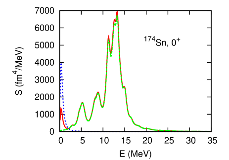
Figure 1: (Color online) Calculated transition strength of the isoscalar monopole $0^{+}$ excitations in ¹⁷⁴Sn (solid red curve), compared with the result in Terasaki1 with the cutoff (iii) (green dashed curve). The transition strength associated to the number operator, magnified by a factor of 10,000, in units of MeV^-1 is shown by the blue dotted curve. See text for details.

In Fig. 1, we compare our results (solid red curve) with the one in Ref. Terasaki1 (dashed green curve). The self-consistent result obtained by Terasaki et al. Terasaki1 also employs the HFB solutions calculated with the HFBRAD. However, in Ref. Terasaki1 , the QRPA matrix is calculated in the canonical-basis representation and an additional truncation of the two-quasi-particle space is introduced for the construction of the QRPA matrix . In contrast, we introduce no additional truncation for our FAM calculation. We compare our results with the one of the cutoff (iii) in Ref. Terasaki1 which takes into account the highest number of states for the construction of the QRPA matrix; all the proton quasi-particles up to 200 MeV and the neutron canonical levels with occupancy $v^{2}>10^{-16}$.

In the first two peaks at $E\sim 5$ and $8.5$ MeV, the two curves are almost perfectly overlapping. The peaks between 11 MeV and 18 MeV occur at the same energy for the two calculations while their height is slightly different. The bump close to zero energy resulting in our calculations has to be attributed to the presence of a spurious mode. To check the position of the spurious mode related to the pairing rotation of the neutrons, we included in Fig. 1 the transition strength associated to the number operator, by the blue dashed line. The spurious mode is well localized close to zero energy.

The present result demonstrates the accuracy and usefulness of the FAM for the superfluid systems. Even if the two codes include some differences in the truncation of the two-quasi-particle space, the similarity of the results is very satisfying

VI Conclusions

The finite amplitude method for the QRPA has been presented. The basic idea is identical to the original FAM fam , that we resort to a numerical differentiation to calculate the induced fields and then solve the linear-response equation with an iterative algorithm such as the GCR. With the FAM, a HFB code with simple modifications can be turned into a QRPA code. Especially, it is very easy to construct the QRPA code which has the same symmetry of the parent HFB one whose subroutines are used to perform the numerical derivative. All the terms present in the TDHFB calculation, including the time-odd mean fields, should be taken into account to construct fully self-consistent codes. This requires us some effort to update the original HFB code. Still, the necessary task for coding the FAM is much less than that for the explicit calculation of the QRPA matrix elements for realistic energy functionals. In addition, it does not require a large memory capacity, since we do not construct the QRPA matrix. We have built a fully self-consistent QRPA code using the HFBRAD BennaDoba . The iterative algorithm, for which we adopted the GCR method in this paper, may be replaced by a better algorithm in future. The resulting strength functions of the isoscalar $0^{+}$ mode of ¹⁷⁴Sn show high similarity with the fully self-consistent calculations in Ref. Terasaki1 . Thus, this paper showed the first application of the FAM for superfluid systems and demonstrated the usefulness of the FAM for the construction of the QRPA code by modifying existing HFB codes.

Appendix A Bogoliubov transformation of one-body fields

A.1 Induced fields $\delta H$

The TDHFB Hamiltonian is given by Eq. (5). We consider the small-amplitude limit, $H(t)=H_{0}+\delta H(t)$, where $H_{0}$ is the HFB Hamiltonian of Eq. (3) and

$$\delta H(t)=\frac{1}{2}\begin{pmatrix}c^{\dagger}&c\end{pmatrix}\begin{pmatrix}\delta h(t)&\delta\Delta(t)\\ -\delta\Delta^{*}(t)&-\delta h^{*}(t)\end{pmatrix}\begin{pmatrix}c\\ c^{\dagger}\end{pmatrix}.$$ (43)

Here, $\delta h(t)$ and $\delta\Delta(t)$ are oscillating as

$$\delta h(t) = \eta\left(\delta h(\omega)e^{-i\omega t}+\delta h^{\dagger}(\omega)e^{i\omega t}\right),$$ (44)

$$\delta\Delta(t) = \eta\left(\delta\Delta^{(+)}(\omega)e^{-i\omega t}+\delta\Delta^{(-)}(\omega)e^{i\omega t}\right).$$ (45)

Note that $\delta\Delta^{(\pm)}(\omega)$ are anti-symmetric but $\delta h(\omega)$ is not necessarily Hermitian. The induced Hamiltonian, Eq. (43), is now expressed in the form of Eq. (8) with $\delta H(\omega)$ given by

$$\delta H(\omega)=\frac{1}{2}\begin{pmatrix}c^{\dagger}&c\end{pmatrix}\begin{pmatrix}\delta h&\delta\Delta^{(+)}\\ -\delta\Delta^{(-)*}&-\delta h^{T}\end{pmatrix}\begin{pmatrix}c\\ c^{\dagger}\end{pmatrix}.$$ (46)

Hereafter, $\delta h(\omega)$ and $\delta\Delta^{(\pm)}(\omega)$ are denoted by $\delta h$ and $\delta\Delta^{(\pm)}$, for simplicity.

Since the Bogoliubov transformation can be written in terms of the unitary matrix $\mathcal{W}$ RS as follows:

$$\begin{pmatrix}a\\ a^{\dagger}\end{pmatrix}=\begin{pmatrix}U^{\dagger}&V^{\dagger}\\ V^{T}&U^{T}\end{pmatrix}\begin{pmatrix}c\\ c^{\dagger}\end{pmatrix}\equiv\mathcal{W^{\dagger}}\begin{pmatrix}c\\ c^{\dagger}\end{pmatrix},$$ (47)

we may rewrite Eq. (46) in the quasi-particle basis:

$$\delta H(\omega)=\frac{1}{2}\begin{pmatrix}a^{\dagger}&a\end{pmatrix}\mathcal{W}^{\dagger}\begin{pmatrix}\delta h&\delta\Delta^{(+)}\\ -\delta\Delta^{(-)*}&-\delta h^{T}\end{pmatrix}\mathcal{W}\begin{pmatrix}a\\ a^{\dagger}\end{pmatrix}.$$ (48)

This transformation should provide $\delta H^{20}$ and $\delta H^{02}$ in Eq. (9).

$$\begin{pmatrix}\delta H^{11}&\delta H^{20}\\ -\delta H^{02}&-(\delta H^{11})^{T}\end{pmatrix}=\mathcal{W}^{\dagger}\begin{pmatrix}\delta h&\delta\Delta^{(+)}\\ -\delta\Delta^{(-)*}&-\delta h^{T}\end{pmatrix}\mathcal{W}.$$ (49)

We write here their explicit expression:

$$\delta H^{20}_{\mu\nu}(\omega) = \left(U^{\dagger}\delta hV^{*}-V^{\dagger}\delta\Delta^{(-)*}V^{*}\right.$$ (50)

$$\quad\left.+U^{\dagger}\delta\Delta^{(+)}U^{*}-V^{\dagger}\delta h^{T}U^{*}\right)_{\mu\nu},$$

$$\delta H^{02}_{\mu\nu}(\omega) = \left(-V^{T}\delta hU+U^{T}\delta\Delta^{(-)*}U\right.$$ (51)

$$\quad\left.-V^{T}\delta\Delta^{(+)}V+U^{T}\delta h^{T}V\right)_{\mu\nu}.$$

A.2 External field $F$

The one-body field in general can be written in a form of Eq. (7) in terms of the quasi-particle operators, neglecting a constant. Suppose that $F(\omega)$ in Eq. (6) has a form

$$F=\sum_{kl}f_{kl}c_{k}^{\dagger}c_{l}=\frac{1}{2}\begin{pmatrix}c^{\dagger}&c\end{pmatrix}\begin{pmatrix}f&0\\ 0&-f^{T}\end{pmatrix}\begin{pmatrix}c\\ c^{\dagger}\end{pmatrix},$$ (52)

where the difference of a constant shift is neglected. Here, the matrix $f_{kl}$ is a general complex matrix, since $F(\omega)$ is non-Hermitian in general. The Bogoliubov transformation as in Eq. (49), then, leads to $F^{20}$ and $F^{02}$ in Eq. (7),

$$F^{20}_{\mu\nu} = \left(U^{\dagger}fV^{*}-V^{\dagger}f^{T}U^{*}\right)_{\mu\nu},$$ (53)

$$F^{02}_{\mu\nu} = \left(U^{T}f^{T}V-V^{T}fU\right)_{\mu\nu}.$$ (54)

In case that $F(\omega)$ has a form of pairing-type

$$F=\frac{1}{2}\sum_{kl}\left(g_{kl}c_{k}^{\dagger}c_{l}^{\dagger}+g^{\prime}_{kl}c_{l}c_{k}\right),$$ (55)

the same calculation provides $F^{20}$ and $F^{02}$ by

$$F^{20}_{\mu\nu} = \left(U^{\dagger}gU^{*}-V^{\dagger}g^{\prime}V^{*}\right)_{\mu\nu},$$ (56)

$$F^{02}_{\mu\nu} = \left(U^{T}g^{\prime}U-V^{T}gV\right)_{\mu\nu}.$$ (57)

References

• (1) P. Ring and P. Schuck: The Nuclear Many Body problem, Springer-Verlag, Berlin (1980).
• (2) M.Bender, P-H. Heneen, P-G. Reinhard, Rev. Mod. Phys. 75, 121 (2003).
• (3) H. Imagawa and Y. Hashimoto, Phys. Rev C 67, 037302 (2003).
• (4) N. Paar, P. Ring, T. Nikšić, and D. Vretenar, Phys. Rev C 67, 034312 (2003).
• (5) T. Nakatsukasa and K. Yabana, Phys. Rev C 71, 024301 (2005).
• (6) J.Terasaki, J. Engel, M. Bender, J. Dobaczewski, Phys. Rev C 71, 034310 (2005).
• (7) S.Fracasso and G. Colò, Phys. Rev C 72, 064310 (2005).
• (8) T. Sil, S. Shlomo, B.K. Agrawal, and P.-G. Reinhard, Phys. Rev C 73, 034316 (2006).
• (9) J.Terasaki and J. Engel, Phys. Rev C 74, 044301 (2006).
• (10) D. P. Artega and P. Ring, Phys. Rev C 77, 034317 (2008).
• (11) S. Péru and H. Goutte, Phys. Rev C 77, 044313 (2008).
• (12) C. Losa, A. Pastore, T. Døssing, E. Vigezzi, R.A. Broglia, Phys. Rev. C 81, 064307 (2010).
• (13) J. Terasaki, J. Engel, Phys. Rev. C 82, 034326 (2010).
• (14) K. Yoshida and N. V. Giai, Phys. Rev. C 78, 064316 (2008).
• (15) K. Yoshida and T. Nakatsukasa, Phys. Rev. C 83, 021304(R) (2011).
• (16) S. Ebata, T. Nakatsukasa, T. Inakura, K. Yoshida, Y. Hashimoto, and K. Yabana, Phys. Rev. C 82, 034306 (2010).
• (17) T. Nakatsukasa, T. Inakura and K. Yabana, Phys. Rev. C 76 024318 (2007).
• (18) T. Inakura, T. Nakatsukasa and K. Yabana, Phys. Rev. C 80 044301 (2009).
• (19) J. Toivanen, B. G. Carlsson, J. Dobaczewski, K. Mizuyama, R.R. Rodríguez-Guzmán, P. Toivanen, P. Veselý, Phys. Rev. C 81, 034312 (2010).
• (20) K. Bennaceur and J. Dobaczewski, Comput. Phys. Comm. 168, 96 (2005).
• (21) Y. Saad: Iterative methods for sparse linear systems, 2nd ed. SIAM, Philadelphia, 2003.
• (22) S.G. Rohozinsky, J. Dobaczewski, W. Nazarevic, Phys. Rev. C 81, 014313 (2010).
• (23) J. Bartel, P. Quentin, M. Brack, C. Guet, and H.B. Håkansson, Nucl. Phys. A386, 79 (1982).
• (24) E. Perlinska, S.G. Rohozinsky, J. Dobaczewski, W. Nazarevic, Phys. Rev. C 69, 014316 (2004).
• (25) J. Dobaczewski, H. Flocard and J. Treiner, Nucl. Phys A422, 103 (1984).