Effect of hydrogen adsorption on the quasiparticle spectra of graphene

Abstract

We use the non-interacting tight-binding model to study the effect of isolated hydrogen adsorbates on the quasiparticle spectra of single-layer graphene. Using the Green’s function approach, we obtain analytic expressions for the local density of states and the spectral function of hydrogen-doped graphene, which are also numerically evaluated and plotted. Our results are relevant for the interpretation of scanning tunneling microscopy and angle-resolved photoemission spectroscopy data of functionalized graphene.

The adsorption of hydrogen on graphene is of fundamental as well as applied significance. Current interest in hydrogenated graphene is due to the possibility of opening a band gap in the semimetallic graphene, which is essential for applications in electronics. This has recently prompted several research groups to experiment with hydrogenated graphene and to study its electronic and transport properties. Elias et al. (2009); Bostwick et al. (2009); Balog et al. (2010); Haberer et al. (2010) Calculations based on density-functional theory (DFT) gave the motivation to search for hydrogenated derivatives of graphene, since they showed that graphane, i.e., the fully hydrogenated compound, is both a stable 2D hydrocarbon and a band insulator. Sofo et al. (2007) Earlier DFT calculations had studied the effect of hydrogen adsorption on the electronic structure of graphene, using a $4\times 4$ regular arrangement, i.e., an H:C ratio of 1:32, and found a band gap opening and the appearance of a spin-polarized dispersionless midgap band. Duplock et al. (2004)

In this work, we analyze the effect of a single hydrogen impurity on the electronic structure of graphene. As we show below, the analysis can be extended also to calculate some properties of randomly distributed H adsorbates at a low-density coverage. A hydrogen atom adsorbed on graphene forms a covalent bond atop a carbon atom, and changes the orbital state of the host atom from $sp^{2}$ to $sp^{3}$. This is expected to have a characteristic effect on the local density of states (LDOS), and to produce Friedel oscillations in the surrounding charge density. These properties can be mapped out by scanning tunneling microscopy (STM) and, indeed, hydrogen monomers and dimers on graphene have been imaged by this technique. Hornekær et al. (2006); Guisinger et al. (2009) As the graphene sample is exposed to a hydrogen plasma, we initially expect the adsorption of a low concentration of randomly distributed H atoms, and in later stages more complicated and perhaps regular adsorption arrangements. We can enumerate several changes that can be expected in the initial stages of adsorption to occur in the quasiparticle spectra. First, due to scattering from the H impurities there is an effect of line broadening in the momentum-resolved spectral function. Second, H adsorption breaks the sublattice symmetry which can lead to a band gap opening at the Dirac point. Third, since hydrogen impurity on graphene acts as a resonant scatterer, a midgap resonance appears in the density of states. Pereira et al. (2006) The spectral function is accessible by angle-resolved photoemission spectroscopy (ARPES), and the above changes have already been obeserved in experiments on hydrogenated graphene. Bostwick et al. (2009); Balog et al. (2010); Haberer et al. (2010)

Theoretical studies of the electronic and transport properties of hydrogenated graphene have been based on a tight-binding model which describes the $\pi$ bands of graphene and an additional orbital for the H adsorbate. Robinson et al. (2008); Wehling et al. (2010); Yuan et al. (2010) The purpose of this Brief Report is to calculate the local density of states and the spectral function of sparsely hydrogenated graphene within the framework of this tight-binding model. As in earlier theoretical studies of the effect of impurities on the spectral properties of graphene, a Green’s function analysis can be used to obtain the desired quantities. Bena and Kivelson (2005); *bena2008; Pereira et al. (2006, 2008); Skrypnyk and Loktev (2006); *skrypnyk2007; Wehling et al. (2007); Feher et al. (2009); Bácsi and Virosztek (2010); Skrypnyk and Loktev (2011) However, in contrast with most previous works which have considered substitional impurities, we deal with adsorbate impurities.

We begin our derivation by defining the non-interacting tight-binding model that describes the $\pi$ bands of graphene with an additional adsorbed hydrogen atom as Robinson et al. (2008); Yuan et al. (2010)

$$\mathcal{H}=\mathcal{H}_{0}+\mathcal{H}_{1}+\mathcal{H}_{2},$$ (1)

where $\mathcal{H}_{0}$ describes pure graphene,

$$\mathcal{H}_{0}=-t\sum_{\langle{i,j}\rangle}c_{i}^{\dagger}c_{j},$$ (2)

$\mathcal{H}_{1}$ describes an isolated hydrogen atom,

$$\mathcal{H}_{1}=\varepsilon_{d}d^{\dagger}d,$$ (3)

and $\mathcal{H}_{2}$ describes the hybridization between graphene and hydrogen adsorbed on an arbitrary host site specified by index $l$,

$$\mathcal{H}_{2}=V(c^{\dagger}_{l}d+d^{\dagger}c_{l}).$$ (4)

Interactions involving spin have not been included in this model, and the spin degree of freedom has been omitted for simplicity. The energy parameters which have been obtained from fits to first-principles band structure calculations are given by $t=2.6$ eV, $V=-2t$ and $\varepsilon_{d}=-t/16$. Wehling et al. (2010)

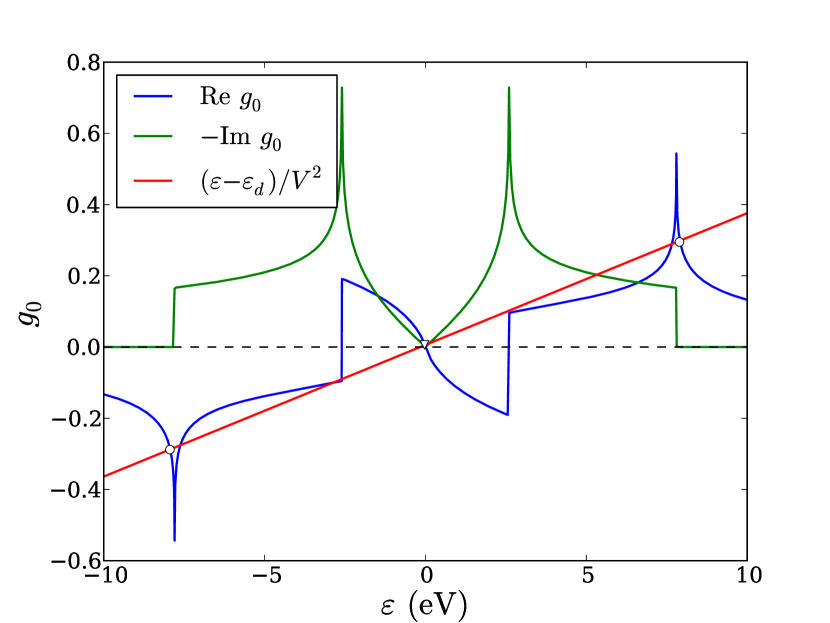
Figure 1: (Color online) Graphical solution of $\varepsilon-\varepsilon_{d}-V^{2}\,\mathrm{Re}\,g_{0}(\varepsilon)=0$ showing the positions of the resonance just to the left of Dirac point, and two localized states just below and above energy bands, respectively.

The local density of states at a given site $m$ is given by

$$\rho(m;\varepsilon)=-\frac{1}{\pi}\mathrm{Im}\,G(m,m;\varepsilon),$$ (5)

where $G(m,m;\varepsilon)$ is a matrix element of the Green’s function $\mathcal{G}(\varepsilon)=(\varepsilon-\mathcal{H}+i0^{+})^{-1}$, while the total DOS of the system is given by

$$\rho(\varepsilon)=-\frac{1}{\pi}\mathrm{Im}\,\mathrm{Tr}\,\mathcal{G}(\varepsilon).$$ (6)

Therefore, we must calculate the Green’s function corresponding to Eq. (1). The crucial step is to consider the graphene or the hydrogen atom as a separate entity, and incorporate the presence of the other system in its Hamiltonian in terms of a self-energy.

The self-energy in a device, is generally given by $\mathcal{V}{g_{R}}\mathcal{V}^{\dagger}$ where $\mathcal{V}$ is the coupling Hamiltonian and $g_{R}$ is the subset of the Green’s function of the reservoir which makes the interface with the device. Datta (2005) Thus instead of Eq. (3), we can describe a hydgrogen atom in contact with graphene by

$$\tilde{\mathcal{H}}_{1}=\left[\varepsilon_{d}+V^{2}g_{0}(\varepsilon)\right]d^{\dagger}d,$$ (7)

where the additional term is the self-energy induced by graphene and $g_{0}(\varepsilon)$ is the diagonal matrix element of the Green’s function of graphene which describes the host site. On the other hand, for graphene in contact with hydrogen, the Hamiltonian becomes Robinson et al. (2008)

$$\tilde{\mathcal{H}}_{0}=-t\sum_{\langle{i,j}\rangle}c_{i}^{\dagger}c_{j}+\frac{V^{2}}{\varepsilon-\varepsilon_{d}}c_{l}^{\dagger}c_{l},$$ (8)

where the additional term is the self-energy induced by hydrogen at the host site, which has the general form if we note that $1/(\varepsilon-\varepsilon_{d})$ is the Green’s function of an isolated hydrogen. We can now calculate the LDOS from the Green’s functions corresponding to Eqs. (7) and (8), respectively. From Eq. (7) it follows that the LDOS at the hydrogen site is given by

$$\rho_{\mathrm{H}}(\varepsilon)=-\frac{1}{\pi}\mathrm{Im}\,\frac{1}{\varepsilon-\varepsilon_{d}-V^{2}g_{0}(\varepsilon)}.$$ (9)

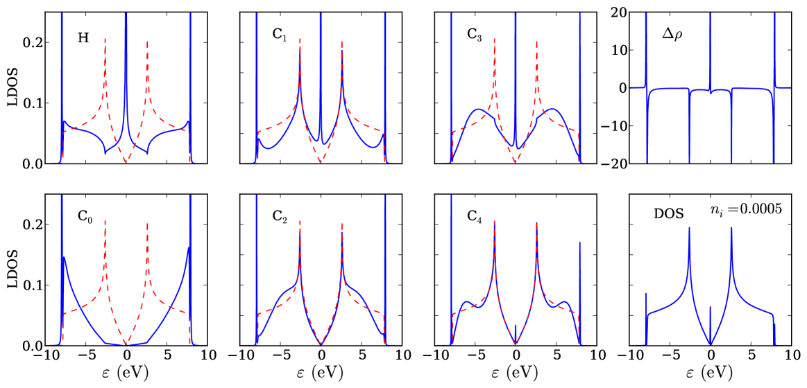
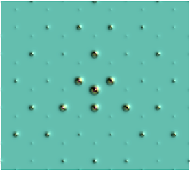
Figure 2: (Color online) Local density of states of graphene with a single hydrogen adsorbate. (Left panel) The subplots show LDOS at the H site, the host site, C₀, and its four nearest neighbors, denoted by C₁–C₄, as well as the change in total DOS of graphene, and the DOS per carbon atom for 0.05% hydrogen coverage. (Right panel) LDOS at the H site (at center) and nearby graphene sites of a rectangular sample of $6\times 6$ unit cells, for an energy near the resonance $\approx-0.03$ eV.

Equation (8) is now similar to the Hamiltonian of a substitutional impurity, with an energy-dependent on-site parameter, so the corresponding Green’s function can be obtained exactly from Economou (2006)

$$\tilde{\mathcal{G}}_{0}=\mathcal{G}_{0}+\mathcal{G}_{0}\mathcal{T}\mathcal{G}_{0},$$ (10)

where the $t$-matrix is given by Robinson et al. (2008)

$$\mathcal{T}=\frac{V^{2}}{\varepsilon-\varepsilon_{d}-V^{2}g_{0}(\varepsilon)}\,c^{\dagger}_{l}{c}_{l}.$$ (11)

We can find the positions of the resonances and localized states by setting the denominators in Eqs. (9) and (11) equal to zero,

$$\varepsilon-\varepsilon_{d}-V^{2}\,\mathrm{Re}\,g_{0}(\varepsilon)=0.$$ (12)

A graphical solution of Eq. (12) is shown in Fig. 1. The position of a solution just to the left of the Dirac point implies a sharp resonance since $\mathrm{Im}\,g_{0}$, which measures the width of the resonance, is vanishingly small. It is to be noted that the strong hybridization between H and C, parameterized as $V$, is responsible for the resonance being much closer to the Dirac point than the on-site energy, $\varepsilon_{d}$. The other solutions of Eq. (12) correspond to two localized states with energies just below and above the band limits, respectively. It is interesting to compare this picture with the case of a vacancy which is also a resonant scatterer. For a vacancy, the equation to solve would change to $1/U=\mathrm{Re}\,g_{0}(\varepsilon)$ where $U$ would now be a large positive constant representing the on-site energy of a vacancy. There will again be a resonance state near the neutrality point, but only one localized state outside the bands at a large positive energy. (cf. Ref. Pereira et al., 2008)

From Eq. (10), it is easy to show that the LDOS at a given site of graphene is given by

$$\rho(m;\varepsilon)=-\frac{1}{\pi}\mathrm{Im}\,\frac{(\varepsilon-\varepsilon_{d})g_{0}+V^{2}(g_{ml}g_{lm}-g_{0}^{2})}{\varepsilon-\varepsilon_{d}-V^{2}g_{0}},$$ (13)

where $g_{ml}\equiv\langle m|\mathcal{G}_{0}|l\rangle$, and for the honeycomb lattice we can use $g_{ml}=g_{lm}$. In particular, for the host site $m=l$, and with $g_{ll}=g_{0}$, we find

$$\rho(l;\varepsilon)=-\frac{1}{\pi}\mathrm{Im}\,\frac{(\varepsilon-\varepsilon_{d})g_{0}}{\varepsilon-\varepsilon_{d}-V^{2}g_{0}}.$$ (14)

When the site $m$ is very far from the host site $l$, $g_{ml}\rightarrow 0$, and $\rho(m;\varepsilon)\rightarrow(-1/\pi)\mathrm{Im}g_{0}(\varepsilon)=\rho_{0}(\varepsilon)$, i.e., it approaches the LDOS of pure graphene.

Evaluation of the LDOS at any lattice site by Eqs. (13) and (14) requires numerical values of the lattice Green’s functions $g_{0}$ and $g_{lm}$, which can be conveniently calculated by the expressions given by Horiguchi in terms of elliptic functions. Horiguchi (1972) In Fig. 2, we have plotted the LDOS at the host site and its four nearest neighbors, which show that the resonance is small on the sites of the sublattice of the host, and large on the other sublattice, which seems to be a common property that is shared by vacancies also. Wehling et al. (2007) Figure 2 shows that at sites farther from the impurity the LDOS approaches that of pure graphene in an oscillatory fashion.

From Eq. (10) it follows that the change in the total DOS of graphene is given by

$$\Delta\rho=\frac{1}{\pi}\mathrm{Im}\left(\frac{dg_{0}}{d\varepsilon}\frac{V^{2}}{\varepsilon-\varepsilon_{d}-V^{2}g_{0}}\right).$$ (15)

To calculate the DOS corresponding to Eq. (1), since we need a finite number of impurities to make the effect finite, we assume to have $N$ carbon atoms in the graphene, and $N_{i}\lll{N}$ well isolated hydrogen adsorbates. We can then write the DOS per carbon site as

$$\rho(\varepsilon)=\rho_{0}(\varepsilon)+n_{i}[\Delta\rho(\varepsilon)+\rho_{\mathrm{H}}(\varepsilon)],$$ (16)

where $\rho_{0}$ is the DOS of pure graphene, and $n_{i}=N_{i}/N$ is the ratio of hydrogen to carbon atoms. A plot of $\rho_{H}$ is shown in Fig. 2 where the expected resonance features can be observed. We have also plotted the change in the total DOS, $\Delta\rho$, and the DOS for graphene with a tiny amount of 0.05% of hydrogen. We note that the total DOS is in agreement with those obtained by numerical calculations. Yuan et al. (2010) It must be remarked that the values of $\Delta\rho$ can become negative while the total DOS must always remain positive. The explanation why this is not unphysical is that the measurable quantity, which is the total DOS, remains positive, because it is of $\mathcal{O}(N)$ while the change in it due to the presence of a single H adsorbate is of $\mathcal{O}(1)$. Also shown in Fig. 2 is the LDOS at the sites of a rectangular sample of $6\times 6$ unit cells of graphene, at an energy near the resonance. This result shows the threefold symmetry and fluctuations of LDOS, and can be related to STM images.

It is easy to extend the above results to find the effect of a low density of H adsorbates on the spectral function, given by

$$A(\mathbf{k},\varepsilon)=\frac{-2\,\mathrm{Im}\,\Sigma(\mathbf{k},\varepsilon)}{[\varepsilon-\varepsilon_{\mathbf{k}}-\mathrm{Re}\,\Sigma(\mathbf{k},\varepsilon)]^{2}+[\mathrm{Im}\,\Sigma(\mathbf{k},\varepsilon)]^{2}},$$ (17)

where $\Sigma(\mathbf{k},\varepsilon)$ is the self-energy due to the presence of hydrogen impurities and $\varepsilon_{\mathbf{k}}$ is the energy dispersion of graphene,

$$\varepsilon_{\mathbf{k}}=\pm t\left[{3+2\left(\cos k_{x}a+2\cos\frac{k_{x}a}{2}\cos\frac{k_{y}a\sqrt{3}}{2}\right)}\right]^{1/2},$$ (18)

where $a=2.46$ Å is graphene lattice constant. For low concentrations of H adsorbates, the average $t$-matrix approximation (ATA) applies and, noting that here we have no explicit $\mathbf{k}$ dependence, we can write

$$\Sigma(\varepsilon)=\frac{n_{i}V^{2}}{\varepsilon-\varepsilon_{d}-V^{2}g_{0}(\varepsilon)}.$$ (19)

The energy and momentum widths of the spectral function at a given energy near the Dirac point can be approximated as $\Delta\varepsilon_{\mathbf{k}}\equiv{\hbar}/\tau_{\mathbf{k}}=-2\,\mathrm{Im}\,\Sigma(\varepsilon_{\mathbf{k}})$, and $\hbar\Delta{k}=-(2/v_{F})\,\mathrm{Im}\,\Sigma(\varepsilon_{\mathbf{k}})$, respectively, where $\tau_{\mathbf{k}}$ is the scattering time and $v_{F}$ is the Fermi velocity. Energy and momentum widths, which are proportional to $n_{i}$ at low concentrations according to Eq. (19), can be deduced from ARPES energy distribution curves (EDC) and momentum distribution curves (MDC), respectively, and can be used to estimate the density of randomly distributed H adsorbates using these results. In Fig. 3, we plot the spectral function for pure graphene and for graphene with a relatively large 2% impurity concentration to make the effects large enough to be more clearly visible. Our plots compare well with the experimental results of Ref. Haberer et al., 2010. We can observe the effect of spectral broadening and the fingerprints of the localized state below the band boundary at $-7.8$ eV. Less trivial are the changes observed around the Dirac point, i.e., the zero energy at $K$ point, where both sublattice symmetry breaking and the presence of the midgap resonance can play a role. Even within the simplest approximation that we have used to relate the many-impurity to the single-impurity scattering, we see a quasi band-gap opening and the appearance of new quasilocalized states within the gap near zero energy. Pereira et al. (2006); Skrypnyk and Loktev (2011)

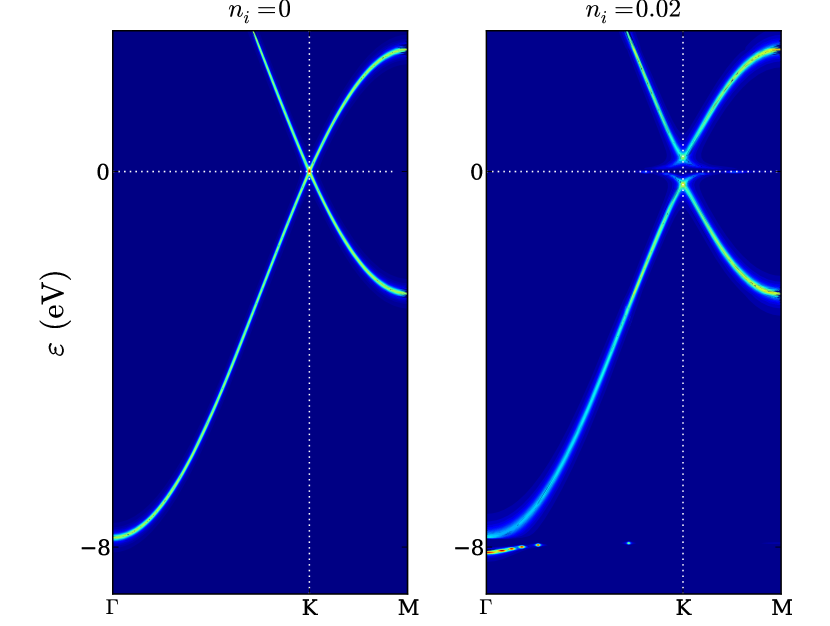
Figure 3: (Color online) Spectral function of graphene along the $\Gamma$KM path of its Brillouin zone. (Left panel) Clean graphene. (Right panel) Graphene with 2% hydrogen adsorption. General line broadening, appearance of a localized state just below the band, and changes similar to a gap opening near zero energy are the noteworthy features.

In conclusion, we presented analytic expressions for the LDOS of graphene with a single hydrogen atom adsorbate, as well as for the spectral function of graphene with a low density of randomly distributed hydrogen adsorbates. Our plots of the spectral function explain the features of quasi band gap and the spectral line broadening observed in angle-resolved photoemission spectra of hydrogenated graphene. Our expressions can be used to estimate the concentration of hydrogen adsorbates from measured spectral linewidths.

We had stimulating discussions with S. A. Jafari. M. F. thanks H. Rafii-Tabar for kind support. A. G. and D. H. acknowledge the DFG Grant No. GR 3708/1-1. A. G. acknowledges an APART fellowship from the Austrian Academy of Sciences.

References

- Elias et al. (2009) D. C. Elias, R. R. Nair, T. M. G. Mohiuddin, S. V. Morozov, P. Blake, M. P. Halsall, A. C. Ferrari, D. W. Boukhvalov, M. I. Katsnelson, A. K. Geim, and K. S. Novoselov, Science 323, 610 (2009).
- Bostwick et al. (2009) A. Bostwick, J. L. McChesney, K. V. Emtsev, T. Seyller, K. Horn, S. D. Kevan, and E. Rotenberg, Phys. Rev. Lett. 103, 056404 (2009).
- Balog et al. (2010) R. Balog, B. Jørgensen, L. Nilsson, M. Andersen, E. Rienks, M. Bianchi, M. Fanetti, E. Lægsgaard, A. Baraldi, S. Lizzit, Z. Slijivancanin, F. Besenbacher, B. Hammer, T. G. Pedersen, P. Hofmann, and L. Hornekær, Nat. Mater. 9, 315 (2010).
- Haberer et al. (2010) D. Haberer, D. V. Vyalikh, S. Taioli, B. Dora, M. Farjam, J. Fink, D. Marchenko, T. Pichler, K. Ziegler, S. Simonucci, M. S. Dresselhaus, M. Knupfer, B. Büchner, and A. Grüneis, Nano Lett. 10, 3360 (2010).
- Sofo et al. (2007) J. O. Sofo, A. S. Chaudhari, and G. D. Barber, Phys. Rev. B 75, 153401 (2007).
- Duplock et al. (2004) E. J. Duplock, M. Scheffler, and P. J. D. Lindan, Phys. Rev. Lett. 92, 225502 (2004).
- Hornekær et al. (2006) L. Hornekær, Ž. Šljivančanin, W. Xu, R. Otero, E. Rauls, I. Stensgaard, E. Lægsgaard, B. Hammer, and F. Besenbacher, Phys. Rev. Lett. 96, 156104 (2006).
- Guisinger et al. (2009) N. P. Guisinger, G. M. Rutter, J. N. Crain, P. N. First, and J. A. Stroscio, Nano Lett. 9, 1462 (2009).
- Pereira et al. (2006) V. M. Pereira, F. Guinea, J. M. B. Lopes dos Santos, N. M. R. Peres, and A. H. Castro Neto, Phys. Rev. Lett. 96, 036801 (2006).
- Robinson et al. (2008) J. P. Robinson, H. Schomerus, L. Oroszlány, and V. I. Fal’ko, Phys. Rev. Lett. 101, 196803 (2008).
- Wehling et al. (2010) T. O. Wehling, S. Yuan, A. I. Lichtenstein, A. K. Geim, and M. I. Katsnelson, Phys. Rev. Lett. 105, 056802 (2010).
- Yuan et al. (2010) S. Yuan, H. De Raedt, and M. I. Katsnelson, Phys. Rev. B 82, 115448 (2010).
- Bena and Kivelson (2005) C. Bena and S. A. Kivelson, Phys. Rev. B 72, 125432 (2005).
- Bena (2008) C. Bena, Phys. Rev. Lett. 100, 076601 (2008).
- Pereira et al. (2008) V. M. Pereira, J. M. B. Lopes dos Santos, and A. H. Castro Neto, Phys. Rev. B 77, 115109 (2008).
- Skrypnyk and Loktev (2006) Y. V. Skrypnyk and V. M. Loktev, Phys. Rev. B 73, 241402(R) (2006).
- Skrypnyk and Loktev (2007) Y. V. Skrypnyk and V. M. Loktev, Phys. Rev. B 75, 245401 (2007).
- Wehling et al. (2007) T. O. Wehling, A. V. Balatsky, M. I. Katsnelson, A. I. Lichtenstein, K. Scharnberg, and R. Wiesendanger, Phys. Rev. B 75, 125425 (2007).
- Feher et al. (2009) A. Feher, I. A. Gospodarev, V. I. Grishaev, K. V. Kravchenko, E. V. Manzheliĭ, E. S. Syrkin, and S. B. Feodos’ev, Low Temp. Phys. 35, 679 (2009).
- Bácsi and Virosztek (2010) Á. Bácsi and A. Virosztek, Phys. Rev. B 82, 193405 (2010).
- Skrypnyk and Loktev (2011) Y. V. Skrypnyk and V. M. Loktev, Phys. Rev. B 83, 085421 (2011).
- Datta (2005) S. Datta, Quantum Transport: Atom to Transistor (Cambridge University Press, Cambridge, 2005).
- Economou (2006) E. N. Economou, Green’s Functions in Quantum Physics, 3rd ed. (Springer-Verlag, Berlin, 2006).
- Horiguchi (1972) T. Horiguchi, J. Math. Phys. 13, 1411 (1972).