Soft-In Soft-Out DFE and Bi-directional DFE

Abstract

We design a soft-in soft-out (SISO) decision feedback equalizer (DFE) that performs better than its linear counterpart in turbo equalizer (TE) setting. Unlike previously developed SISO-DFEs, the present DFE scheme relies on extrinsic information formulation that directly takes into account the error propagation effect. With this new approach, both error rate simulation and the extrinsic information transfer (EXIT) chart analysis indicate that the proposed SISO-DFE is superior to the well-known SISO linear equalizer (LE). This result is in contrast with the general understanding today that the error propagation effect of the DFE degrades the overall TE performance below that of the TE based on a LE. We also describe a new extrinsic information combining strategy involving the outputs of two DFEs running in opposite directions, that explores error correlation between the two sets of DFE outputs. When this method is combined with the new DFE extrinsic information formulation, the resulting “bidirectional” turbo-DFE achieves excellent performance-complexity tradeoffs compared to the TE based on the BCJR algorithm or on the LE. Unlike turbo LE or turbo DFE, the turbo BiDFE’s performance does not degrade significantly as the feedforward and feedback filter taps are constrained to be time-invariant.

I Introduction

Intersymbol interference (ISI) arises as the transmitted symbols overlaps with one another in high speed digital communication. Powerful modern equalization methods are based on the turbo equalization principle established in [1], wherein a soft-in soft-out (SISO) equalizer (or detector) and a SISO error-correction decoder exchange soft information in an iterative fashion until reliable decisions are generated. It has been shown in [1] that even for some heavy ISI channels the detrimental effect of ISI disappears with this approach.

The detector or the equalizer portion of a turbo equalizer (TE) system often investigated is based on the well-known Bahl-Cocke-Jelinek-Raviv (BCJR) algorithm [2]. This algorithm exactly computes the a posteriori probability (APP) of the transmitted signal symbols considering the channel response and the a priori information of the transmitted symbols and, as such, can be viewed as an optimum SISO equalizer. However, the computational complexity of this algorithm grows exponentially as a function of the channel length and the symbol alphabet set size.

The high computational complexity of the BCJR-based equalizer has motivated considerable research on numerous suboptimal but low complexity equalization schemes. A notable development along this direction is the well-known SISO linear equalizer (LE) of [3]. Another possibility, which was also evaluated in [3], is the SISO decision feedback equalizer (DFE). In the classical, non-turbo setting (i.e., no iterative exchange of soft information between the equalizer and the decoder), it has long been known that the DFE almost always outperforms the LE, despite the fact that the DFE typically suffers from error propagation. This is because when ISI is severe with the channel response showing nulls or deep valleys within the Nyquist band, the LE is subject to large noise enhancement. The work of [3], however, shows that when hard decisions are fed through the feedback filter (to reduce complexity), SISO-DFE performs considerably worse than SISO-LE, presumably due to error propagation.

In classical DFE setting, many techniques have been investigated to mitigate error propagation [4], [5], [6]. Recently, it has been shown [7], [8], [9] that conducting both normal and time-reversed equalization of the received data sequence with two DFEs running in opposite directions and combining two DFE outputs is very effective in reducing error propagation and improving bit error rate (BER) performance. This “bi-directional” DFE (called BiDFE) algorithm takes advantage of the different decision error and noise distributions at the outputs of the forward and time-reversed DFEs [7], [8].

The contribution of this paper is two-fold. One is that this paper readdresses the DFE design issue in the turbo equalizer environment and shows that just as in classical non-turbo setting, the DFE outperforms the LE, if extrinsic information is reformulated in a way that combats error propagation more effectively. The second contribution is a specific DFE extrinsic information combining strategy applied to a BiDFE that suppresses statistical correlation between the outputs of two opposite direction DFEs. We show that the resulting turbo BiDFE performance approaches the performance of the BCJR-based turbo equalizer in a fairly severe ISI environment, easily outperforming the turbo equalizer based on the SISO-LE of [3]. Remarkably, the performance of a time-invariant version of the BiDFE, a lower-complexity method that does not require tap-weight updating as a function of time, also consistently is better than the SISO-LE scheme of [3] based on a time-varying linear filter. There also exist feedback equalization techniques that utilize soft decisions to reduce error propagation [6], [9], [10], [11] but we focus on hard-decision feedback in this paper, as the feedback finite-impulse-response filter complexity is greatly reduced when feedback decisions are constrained to take hard values.

The remainder of the paper is organized as follows. In Section II, a brief statement of the problem is given. In Section III, we give a quick review of the SISO equalizer design method established in [3] and then provide a new formulation of the extrinsic information of DFE taking into account the error propagation effect. We also provide the mean-squared-error analysis of the infinite-length BiDFE in Section IV. The iterative BiDFE algorithm is introduced with the extrinsic information combiner of the normal forward and time-reversed DFE outputs in Section V. In Section VI, numerical results and analysis are given. Finally, we draw conclusions in Section VII.

II System Model

We assume that the receiver knows the discrete-time baseband channel response accurately. While the methods discussed are general, our presentation will be based on binary symbols with $P_{x}\triangleq\mathrm{E}(x_{n}^{2})=1$, $x_{n}\in\{\pm 1\}$, as well as real-valued ISI channel coefficients and noise samples. Although $x_{n}$ typically represents a coded bit sequence, our analysis will assume that it is equiprobable and independent and identically distributed (i.i.d.). Given the transmitted bit sequence $\{x_{k}\}$, the channel output at time $n$ is

$$r_{n} = \sum_{k=0}^{L_{h}-1}{h_{k}x_{n-k}}+w_{n}$$ (1)

where $w_{n}$ is additive white Gaussian noise (AWGN) with variance $N_{0}$ and $\{h_{k}\}$ is the channel impulse response with length $L_{h}$.

In turbo equalization, the equalizer computes the a posteriori log-likelihood ratio (LLR) of $x_{n}$,

$$L(x_{n})\triangleq\ln\dfrac{\mathrm{Pr}(x_{n}=+1\mid\mathbf{r}_{n})}{\mathrm{Pr}(x_{n}=-1\mid\mathbf{r}_{n})}$$

where $\mathbf{r}_{n}$ is the received sample block utilized for LLR estimation for $x_{n}$. Note that this computation requires the knowledge of the a priori probabilities of all input bits affecting $\mathbf{r}_{n}$. Since these a priori probabilities are not available, they are all set to 1/2 initially and then, as the turbo iteration ensues, to the estimated probability values based on the extrinsic information generated and passed back by the outer decoder.

The equalizer then generates its own extrinsic information by subtracting the effect of the probability estimate passed down for the current bit. Write this estimated a priori LLR passed down from the decoder as

$$L_{a}(x_{n})\triangleq\ln\dfrac{\mathrm{Pr}(x_{n}=+1)}{\mathrm{Pr}(x_{n}=-1)}$$

with an understanding that the probabilities in the expression are in reality just estimates.

Then, the equalizer’s extrinsic LLR for $x_{n}$ to be passed to the error-correction code decoder is given by

$$L_{e}(x_{n})\triangleq L(x_{n})-L_{a}(x_{n}).$$

This equation suggests first computing $L(x_{n})$ based on the a priori probabilities of all input bits including $x_{n}$ and then simply subtracting $L_{a}(x_{n})$ to generate the extrinsic LLR $L_{e}(x_{n})$. An alternative way of generating $L_{e}(x_{n})$ is to set $L_{a}(x_{n})=0$ while computing $L(x_{n})$, i.e., suppress the effect of $L_{a}(x_{n})$ in the calculation of $L(x_{n})$:

$$L_{e}(x_{n})=L(x_{n})|_{L_{a}(x_{n})=0}.$$

The techniques discussed in this paper actually use the second method.

III Derivation of Modified Iterative DFE Algorithm

In this section we first briefly review the results of [3] related to the SISO-DFE to provide necessary background while establishing notation. We then show a new way of computing extrinsic information so as to suppress error propagation and improve performance.

III-A Review of Existing Extrinsic LLR Mapping

The work of [3] has established an effective strategy of utilizing the a priori information estimates from the outer decoder in calculating the equalizer tap coefficients. The gist of the approach in [3] is a clever tweaking of the classical minimum-mean-squared-error (MMSE) estimation principle where the “mean” of the input symbols are constructed using the available a priori information estimates and utilized in the linear estimator weight computation. Both the LE and the DFE can be designed in this way, but we shall focus on the DFE here. Based on the above principle and suppressing the effect of the a priori probability estimate on the current bit $x_{n}$ (i.e., $\mathrm{E}(x_{n})=0$) in an effort to extract the extrinsic information, the MMSE feedforward filter taps (a total of $L_{c}+1$) and the feedback filter taps (a total of $L_{d}=L_{h}-1$) at time $n$ are derived respectively as:

$$\mathbf{c}_{n} \triangleq \left[{c_{\{n,0\}},c_{\{n,+1\}},\ldots,c_{\{n,L_{c}\}}}\right]^{T}$$ (2)

$$= \left\{{\mathbf{H}\mathbf{\Sigma}_{n}\mathbf{H}^{T}+(1-z_{n})\mathbf{s}\mathbf{s}^{T}+N_{0}\mathbf{I}}\right\}^{-1}\mathbf{s}$$

$$\mathbf{d}_{n} \triangleq \left[{d_{\{n,-L_{d}\}},d_{\{n,-L_{d}+1\}},\ldots,d_{\{n,-1\}}}\right]^{T}$$ (3)

$$= \mathbf{M}\mathbf{H}^{T}\mathbf{c}_{n}$$

where $\mathbf{H}$ is a channel convolution matrix defined as

$$\mathbf{H}\triangleq\left[{\begin{array}[]{*{20}c}{h_{L_{h}-1}}&{h_{L_{h}-2}}&\cdots&{h_{0}}&0&\cdots&{}\hfil&0\\ 0&{h_{L_{h}-1}}&{h_{L_{h}-2}}&\cdots&{h_{0}}&0&\cdots&0\\ {}\hfil&\ddots&{}\hfil&\ddots&{}\hfil&\ddots&{}\hfil&{}\hfil\\ 0&0&\cdots&0&{h_{L_{h}-1}}&{h_{L_{h}-2}}&\cdots&{h_{0}}\\ \end{array}}\right]$$

and the matrix $\mathbf{\Sigma}_{n}$ depends on $\mathrm{E}(x_{i})$, $i=n,n+1,...,n+L_{c}$, computed from the decoder output as $\mathrm{E}(x_{i})=\tanh(L_{a}(x_{i})/2)$. Specifically, $\mathbf{\Sigma}_{n}\triangleq{\mathrm{Diag}}(\mathbf{0}_{1\times L_{d}},z_{n},z_{n+1},\ldots,z_{n+L_{c}})$ with $z_{i}\triangleq 1-[\mathrm{E}(x_{i})]^{2}$. Adding the term $(1-z_{n})\mathbf{s}\mathbf{s}^{T}$ in (2) has the same effect of suppressing $\mathrm{E}(x_{n})$ to zero in $\mathbf{H}\mathbf{\Sigma}_{n}\mathbf{H}^{T}$. The remaining vector and matrix are defined as ${\mathbf{s}}\triangleq{\mathbf{H}}[\mathbf{0}_{1\times L_{d}},1,\mathbf{0}_{1\times L_{c}}]^{T}$ and $\mathbf{M}\triangleq[\mathbf{I}_{L_{d}\times L_{d}},\mathbf{0}_{L_{d}\times(L_{c}+1)}]$.

The equalizer output is obtained as

$$y_{n} = \mathbf{c}_{n}^{T}\cdot\left(\mathbf{r}_{n}-\mathbf{H}\bar{\mathbf{x}}_{n}+\mathrm{E}(x_{n})\mathbf{s}\right)$$ (4)

where the received vector is defined as $\mathbf{r}_{n}\triangleq\left[{r_{n},r_{n+1},\ldots,r_{n+L_{c}}}\right]^{T}$ and the composite vector of the causal symbol decisions and the anticausal symbols’ mean as $\bar{\mathbf{x}}_{n}\triangleq\left[\hat{x}_{n-L_{d}},\ldots,\hat{x}_{n-1},\mathrm{E}(x_{n}),\ldots,\mathrm{E}(x_{n+L_{c}})\right]^{T}$ where $\hat{x}_{i}$ is the available decision for $x_{i}$ based on the a posteriori LLR of $x_{i}$, i.e., if $L(x_{i})=L_{a}(x_{i})+L_{e}(x_{i})\geq 0$, then, $\hat{x}_{i}=+1$; otherwise, $\hat{x}_{i}=-1$. The addition of the $\mathrm{E}(x_{n})\mathbf{s}$ term is also to suppress the effect of $\mathrm{E}(x_{n})$ in $\mathbf{H}\bar{\mathbf{x}}_{n}$.

Define the anticausal symbol sequence $\mathbf{x}_{n}\triangleq\left[{x_{n},x_{n+1},\ldots,x_{n+L_{c}}}\right]^{T}$, the causal symbol sequence $\mathbf{x}^{c}_{n}\triangleq\left[{x_{n-L_{d}},x_{n-L_{d}+1},\ldots,x_{n-1}}\right]^{T}$, and the available decision sequence $\mathbf{\hat{x}}^{c}_{n}\triangleq\left[{\hat{x}_{n-L_{d}},\hat{x}_{n-L_{d}+1},\ldots,\hat{x}_{n-1}}\right]^{T}$. Also define the noise sequence as $\mathbf{w}_{n}\triangleq\left[{w_{n},w_{n+1},\ldots,w_{n+L_{c}}}\right]^{T}$. Then, the combined filter output $y_{n}$ can be rewritten as

$$y_{n} = (\mathbf{c}^{T}_{n}\mathbf{H}_{1})\cdot\big{(}\mathbf{x}_{n}-\mathrm{E}\{\mathbf{\dot{x}}_{n}\}\big{)}+\mathbf{d}_{n}^{T}(\mathbf{x}^{c}_{n}-\mathbf{\hat{x}}^{c}_{n})+\mathbf{c}^{T}_{n}\mathbf{w}_{n}$$ (5)

$$= p_{\{n,0\}}x_{n}+\sum\limits_{k=1}^{L_{d}}d_{\{n,-k\}}\big{(}{x_{n-k}-\hat{x}_{n-k}}\big{)}+\sum\limits_{k=1}^{L_{c}}{p_{\{n,k\}}\big{(}{x_{n+k}-\mathrm{E}(x_{n+k})}\big{)}}+\sum\limits_{k=0}^{L_{c}}c_{\{n,k\}}w_{n+k}$$

$$= p_{\{n,0\}}x_{n}+i_{n}+v_{n}$$

where $\mathrm{E}\{\mathbf{\dot{x}}_{n}\}\triangleq\left[{0,\mathrm{E}(x_{n+1}),\mathrm{E}(x_{n+2}),\ldots,\mathrm{E}(x_{n+L_{c}})}\right]^{T}$ and $\mathbf{H}_{1}$ is the $(L_{c}+1)\times(L_{c}+1)$ submatrix of $\mathbf{H}$ formed by the entire rows of the columns from the $(L_{d}+1)$th to the last. Moreover, $\mathbf{p}_{n}\triangleq\left[{p_{\{n,0\}},p_{\{n,1\}},\ldots,p_{\{n,L_{c}\}}}\right]=\mathbf{c}_{n}^{T}\mathbf{H}_{1}$ and $p_{\{n,0\}}=\mathbf{c}^{T}_{n}\mathbf{s}$. The error propagation caused by the mismatched hard decision feedback is denoted as $i_{n}$, i.e., $i_{n}\triangleq\sum_{k=1}^{L_{d}}d_{\{n,-k\}}\big{(}{x_{n-k}-\hat{x}_{n-k}}\big{)}$ and $v_{n}$ is the sum of noise and the remaining ISI terms caused by the neighboring symbols: $v_{n}\triangleq\sum_{k=1}^{L_{c}}{p_{\{n,k\}}\big{(}{x_{n+k}-\mathrm{E}(x_{n+k})}\big{)}}+\sum_{k=0}^{L_{c}}c_{\{n,k\}}w_{n+k}$. The variance of $v_{n}$ is

$$\mathrm{Var}(v_{n}) \triangleq \mathbf{c}_{n}^{T}\mathrm{Cov}\{\mathbf{r}_{n}\mathbf{r}_{n}^{T}\mid x_{n}=x\}\mathbf{c}_{n}$$ (6)

$$= \mathbf{c}_{n}^{T}\mathbf{s}(1-\mathbf{s}^{T}\mathbf{c}_{n}).$$

Assuming that the feedback decisions are all correct, i.e., $i_{n}=0$, and $v_{n}$ is AWGN, the extrinsic LLR is naturally given by

$$L_{e}(x_{n}) \triangleq \ln\dfrac{\mathrm{Pr}(x_{n}=+1\mid y_{n})}{\mathrm{Pr}(x_{n}=-1\mid y_{n})}\Bigg{|}_{L_{a}(x_{n})=0}$$ (7)

$$= \ln\dfrac{\mathrm{Pr}(y_{n}\mid x_{n}=+1)\mathrm{Pr}(x_{n}=+1)}{\mathrm{Pr}(y_{n}\mid x_{n}=-1)\mathrm{Pr}(x_{n}=-1)}\Bigg{|}_{L_{a}(x_{n})=0}$$

$$= \ln\dfrac{\mathrm{Pr}(y_{n}\mid x_{n}=+1)}{\mathrm{Pr}(y_{n}\mid x_{n}=-1)}$$

$$= -\dfrac{\left|y_{n}-p_{\{n,0\}}\right|^{2}}{2\mathrm{Var}(v_{n})}+\dfrac{\left|y_{n}+p_{\{n,0\}}\right|^{2}}{2\mathrm{Var}(v_{n})}$$

$$= \dfrac{2p_{\{n,0\}}y_{n}}{\mathrm{Var}(v_{n})}.$$

Notice that in generating $y_{n}$, $L_{a}(x_{n})$ was already suppressed to zero.

A glossary of frequently used symbols is given below. Time-varying quantities are augmented with time index $n$ as the subscript.

$\mathbf{c}_{n}$	DFE feedforward filter coefficients of length $L_{c}+1$	$x_{n}$	transmitted symbol
$\mathbf{d}_{n}$	DFE feedback filter coefficients of length $L_{d}$	$w_{n}$	channel noise
$\mathbf{H}$	channel convolution matrix	$P_{x}$	average power of $x_{n}$
$\mathbf{M}$	$[\mathbf{I}_{L_{d}\times L_{d}},\mathbf{0}_{L_{d}\times(L_{c}+1)}]$	$N_{0}$	variance of $w_{n}$
$\mathbf{s}$	$\mathbf{H}[\mathbf{0}_{1\times L_{d}},1,\mathbf{0}_{1\times L_{c}}]^{T}$	$\{h_{k}\}$	ISI channel response of length $L_{h}$
$\mathbf{p}_{n}$	$\mathbf{c}_{n}^{T}\mathbf{H}_{1}$ where $\mathbf{H}_{1}$ is a submatrix of $\mathbf{H}$	$r_{n}$	received channel output
$\mathbf{r}_{n}$	received sample vector	$y_{n}$	equalized observation
$\bar{\mathbf{x}}_{n}$	vector of causal decisions and anticausal’s mean	$i_{n}$	error due to mismatched past decisions
$\mathbf{w}_{n}$	noise sample vector	$v_{n}$	noise plus error due to pre-cursor ISI
$\mathbf{x}_{n}$	transmitted anticausal symbol vector	$p_{\{n,0\}}$	weight on $x_{n}$ in $y_{n}$
$\mathbf{x}^{c}_{n}$	transmitted causal symbol vector	$L_{a}(x_{n})$	a priori LLR of $x_{n}$
$\mathbf{\hat{x}}^{c}_{n}$	estimated causal symbol vector	$L(x_{n})$	a posteriori LLR of $x_{n}$
$\mathbf{y}^{c}_{n}$	equalized causal sample vector	$L_{e}(x_{n})$	extrinsic LLR of $x_{n}$
$\mathbf{e}^{c}_{\{n,j\}}$	possible causal error sequence	$z_{n}$	variance of $x_{n}$
$\mathbf{\Sigma}_{n}$	covariance matrix of transmitted anticausal symbols	$\acute{z}_{n}$	variance of $x_{n}$ estimated via a posteriori LLR
$\mathbf{\acute{\Sigma}^{c}}_{n}$	covariance matrix of estimated causal symbols	$\rho_{n}$	noise correlation coefficient between two DFEs

III-B New Formulation of Extrinsic Information

While the MAP estimation of $i_{n}$ is equal to zero, we observe that the chance of $i_{n}\neq 0$ is relatively high for severe ISI channels. Our strategy is to estimate $i_{n}$ and utilize the statistical parameters associated with this estimate in the formulation of the extrinsic information. Since $i_{n}$ is to be estimated on the basis of the observation $\mathbf{y}^{c}_{n}\triangleq[y_{n-L_{d}},y_{n-L_{d}+1},\ldots,y_{n-1}]^{T}$, the mean and variance of $i_{n}$ can be evaluated by the a posteriori probabilities of the causal symbols. Write

$$\mathrm{E}(i_{n}) \triangleq \mathrm{E}\left\{\mathbf{d}^{T}_{n}(\mathbf{x}^{c}_{n}-\mathbf{\hat{x}}^{c}_{n})\mid\mathbf{y}^{c}_{n}\right\}$$ (8)

$$= \mathbf{d}_{n}^{T}\left(\tanh(L(\mathbf{x}^{c}_{n})/2)-\mathbf{\hat{x}}^{c}_{n}\right)$$

$$\mathrm{Var}(i_{n}) \triangleq \mathrm{Var}\left\{\mathbf{d}^{T}_{n}(\mathbf{x}^{c}_{n}-\mathbf{\hat{x}}^{c}_{n})\mid\mathbf{y}^{c}_{n}\right\}$$ (9)

$$= \mathbf{d}^{T}_{n}\mathbf{\acute{\Sigma}}^{c}_{n}\mathbf{d}_{n}$$

where $L(\mathbf{x}^{c}_{n})=[L(x_{n-L_{d}}),L(x_{n-L_{d}+1}),\ldots,L(x_{n-1})]^{T}$, $\mathbf{\acute{\Sigma}}^{c}_{n}\triangleq\mathrm{Diag}\left(\acute{z}_{n-L_{d}},\acute{z}_{n-L_{d}+1},\ldots,\acute{z}_{n-1}\right)$, and $\acute{z}_{n}=1-\tanh(L(x_{n})/2)^{2}$.

Now, let us consider the possible causal error sequence $\mathbf{e}^{c}_{\{n,j\}}\triangleq\mathbf{x}^{c}_{\{n,j\}}-\mathbf{\hat{x}}^{c}_{n}$ for $j=1,2,\ldots,2^{L_{d}}$, with index $j$ pointing to a particular binary pattern of $\mathbf{x}^{c}_{n}$. Then, we can compute the extrinsic information for the given causal error sequence $\mathbf{e}^{c}_{\{n,j\}}$:

$$L_{e}(x_{n}|\mathbf{e}^{c}_{\{n,j\}}) \triangleq \ln\dfrac{\mathrm{Pr}(y_{n}\mid x_{n}=+1,\mathbf{e}^{c}_{\{n,j\}})}{\mathrm{Pr}(y_{n}\mid x_{n}=-1,\mathbf{e}^{c}_{\{n,j\}})}$$ (10)

$$= \dfrac{2p_{\{n,0\}}(y_{n}-\mathbf{d}_{n}^{T}\mathbf{e}^{c}_{\{n,j\}})}{\mathrm{Var}(v_{n})}.$$

To compute the extrinsic information of $x_{n}$ taking into account the probabilities of possible error sequences, we write

$$\mathrm{Pr}(y_{n}\mid x_{n}=+1) = \sum_{j=1}^{2^{L_{d}}}\mathrm{Pr}(y_{n}\mid x_{n}=+1,\mathbf{e}^{c}_{\{n,j\}})\mathrm{Pr}(\mathbf{e}^{c}_{\{n,j\}})$$ (11)

$$= \sum_{j=1}^{2^{L_{d}}}\dfrac{\exp\left(L_{e}(x_{n}|\mathbf{e}^{c}_{\{n,j\}})\right)\mathrm{Pr}(\mathbf{e}^{c}_{\{n,j\}})}{1+\exp\left(L_{e}(x_{n}|\mathbf{e}^{c}_{\{n,j\}})\right)}$$

$$\mathrm{Pr}(y_{n}\mid x_{n}=-1) = \sum_{j=1}^{2^{L_{d}}}\mathrm{Pr}(y_{n}\mid x_{n}=-1,\mathbf{e}^{c}_{\{n,j\}})\mathrm{Pr}(\mathbf{e}^{c}_{\{n,j\}})$$ (12)

$$= \sum_{j=1}^{2^{L_{d}}}\dfrac{\mathrm{Pr}(\mathbf{e}^{c}_{\{n,j\}})}{1+\exp\left(L_{e}(x_{n}|\mathbf{e}^{c}_{\{n,j\}})\right)}.$$

Accordingly, the extrinsic information of $x_{n}$ considering the distribution of $i_{n}$ is given as

$$L_{e}(x_{n}) = \ln\left\{\sum\limits_{j=1}^{2^{L_{d}}}\dfrac{\exp\left(L_{e}(x_{n}|\mathbf{e}^{c}_{\{n,j\}})\right)\mathrm{Pr}(\mathbf{e}^{c}_{\{n,j\}})}{1+\exp\left(L_{e}(x_{n}|\mathbf{e}^{c}_{\{n,j\}})\right)}\right\}-\ln\left\{\sum\limits_{j=1}^{2^{L_{d}}}\dfrac{\mathrm{Pr}(\mathbf{e}^{c}_{\{n,j\}})}{1+\exp\left(L_{e}(x_{n}|\mathbf{e}^{c}_{\{n,j\}})\right)}\right\}.$$ (13)

In principle, the extrinsic information of (13) can be evaluated using (10) and approximating $\mathrm{Pr}(\mathbf{e}^{c}_{\{n,j\}})$ or $\mathrm{Pr}(\mathbf{e}^{c}_{\{n,j\}}|\mathbf{y}_{n}^{c})$ by $\prod_{k=1}^{L_{d}}\mathrm{Pr}(e_{\{n-k,j\}}|y_{n-k})$, which can be computed based on the a posteriori LLRs of $\mathbf{x}^{c}_{n}$.

However, since the computational complexity of (13) increases exponentially according to the length of feedback filter, $L_{d}$, we seek a more practical modification. A possible solution is to apply the Bayes’ rule only for the two mutually exclusive cases of $i_{n}=0$ and $i_{n}\neq 0$. Then,

$$\mathrm{Pr}(y_{n}\mid x_{n}=+1) = \dfrac{\exp\left(L_{e}(x_{n}|i_{n}=0)\right)\mathrm{Pr}(i_{n}=0)}{1+\exp\left(L_{e}(x_{n}|i_{n}=0)\right)}+\dfrac{\exp\left(L_{e}(x_{n}|i_{n}\neq 0)\right)\mathrm{Pr}(i_{n}\neq 0)}{1+\exp\left(L_{e}(x_{n}|i_{n}\neq 0)\right)}$$ (14)

$$\mathrm{Pr}(y_{n}\mid x_{n}=-1) = \dfrac{\mathrm{Pr}(i_{n}=0)}{1+\exp\left(L_{e}(x_{n}|i_{n}=0)\right)}+\dfrac{\mathrm{Pr}(i_{n}\neq 0)}{1+\exp\left(L_{e}(x_{n}|i_{n}\neq 0)\right)}.$$ (15)

The extrinsic information of $x_{n}$ for each case of $i_{n}$ can be estimated as

$$L_{e}(x_{n}|i_{n}=0) = \dfrac{2p_{\{n,0\}}y_{n}}{\mathrm{Var}(v_{n})}$$ (16)

$$L_{e}(x_{n}|i_{n}\neq 0) = \ln\left\{\sum\limits_{j=1,\mathbf{e}^{c}_{\{n,j\}}\neq\mathbf{0}}^{2^{L_{d}}}\dfrac{\exp\left(L_{e}(x_{n}|\mathbf{e}^{c}_{\{n,j\}})\right)\mathrm{Pr}(\mathbf{e}^{c}_{\{n,j\}})}{\left\{1+\exp\left(L_{e}(x_{n}|\mathbf{e}^{c}_{\{n,j\}})\right)\right\}\mathrm{Pr}(i_{n}\neq 0)}\right\}$$

$$-\ln\left\{\sum\limits_{j=1,\mathbf{e}^{c}_{\{n,j\}}\neq\mathbf{0}}^{2^{L_{d}}}\dfrac{\mathrm{Pr}(\mathbf{e}^{c}_{\{n,j\}})}{\left\{1+\exp\left(L_{e}(x_{n}|\mathbf{e}^{c}_{\{n,j\}})\right)\right\}\mathrm{Pr}(i_{n}\neq 0)}\right\}$$

$$\simeq \ln\left\{\sum\limits_{j=1,\mathbf{e}^{c}_{\{n,j\}}\neq\mathbf{0}}^{2^{L_{d}}}\left(\dfrac{1}{2}+\dfrac{L_{e}(x_{n}|\mathbf{e}^{c}_{\{n,j\}})}{4}\right)\dfrac{\mathrm{Pr}(\mathbf{e}^{c}_{\{n,j\}})}{\mathrm{Pr}(i_{n}\neq 0)}\right\}$$

$$-\ln\left\{\sum\limits_{j=1,\mathbf{e}^{c}_{\{n,j\}}\neq\mathbf{0}}^{2^{L_{d}}}\left(\dfrac{1}{2}-\dfrac{L_{e}(x_{n}|\mathbf{e}^{c}_{\{n,j\}})}{4}\right)\dfrac{\mathrm{Pr}(\mathbf{e}^{c}_{\{n,j\}})}{\mathrm{Pr}(i_{n}\neq 0)}\right\}$$

$$= \ln\left\{\mathop{\mathrm{missing}}{E}\limits_{i_{n}}\left(\dfrac{1}{2}+\dfrac{2p_{\{n,0\}}\left(y_{n}-i_{n}\right)}{4\mathrm{Var}(v_{n})}\Bigg{|}i_{n}\neq 0\right)\right\}-\ln\left\{\mathop{\mathrm{missing}}{E}\limits_{i_{n}}\left(\dfrac{1}{2}-\dfrac{2p_{\{n,0\}}\left(y_{n}-i_{n}\right)}{4\mathrm{Var}(v_{n})}\Bigg{|}i_{n}\neq 0\right)\right\}$$

$$= \ln\left\{1+\dfrac{p_{\{n,0\}}\left(y_{n}-\mathrm{E}(i_{n}|i_{n}\neq 0)\right)}{\mathrm{Var}(v_{n})}\right\}-\ln\left\{1-\dfrac{p_{\{n,0\}}\left(y_{n}-\mathrm{E}(i_{n}|i_{n}\neq 0)\right)}{\mathrm{Var}(v_{n})}\right\}$$

$$\simeq \left\{{\begin{array}[]{*{20}c}{2\varphi_{n}/(1-\varphi_{n})\textrm{ if $\varphi_{n}<0$ }}\\ {2\varphi_{n}/(1+\varphi_{n})\textrm{ otherwise}}\\ \end{array}}\right.$$ (20)

$$= \dfrac{2\varphi_{n}}{1+|\varphi_{n}|}$$ (21)

where $\varphi_{n}\triangleq{p_{\{n,0\}}\left(y_{n}-\mathrm{E}(i_{n}|i_{n}\neq 0)\right)}/{\mathrm{Var}(v_{n})}$, $\mathrm{E}(i_{n}|i_{n}\neq 0)=\mathrm{E}(i_{n})/\mathrm{Pr}(i_{n}\neq 0)$, $\mathrm{Pr}(i_{n}=0)=\prod_{k=1}^{L_{d}}\exp(|L(x_{n-k})|)/(1+\exp(|L(x_{n-k})|))$, and $\mathrm{Pr}(i_{n}\neq 0)=1-\mathrm{Pr}(i_{n}=0)$. The approximation of (III-B) is from the first order Taylor expansion at zero, i.e, $e^{x}/(1+e^{x})\simeq 0.5+0.25x$ and $1/(1+e^{x})\simeq 0.5-0.25x$. Furthermore, we also use $\ln\left\{1+\varphi_{n}\right\}-\ln\left\{1-\varphi_{n}\right\}=\ln\left\{1+2\varphi_{n}/(1-\varphi_{n})\right\}=-\ln\left\{1-2\varphi_{n}/(1+\varphi_{n})\right\}$ and $\ln(1+x)\simeq x$ in (20). In other words, $\ln\left\{1+2\varphi_{n}/(1-\varphi_{n})\right\}\simeq 2\varphi_{n}/(1-\varphi_{n})$ is used for $\varphi_{n}<0$ while $-\ln\left\{1-2\varphi_{n}/(1+\varphi_{n})\right\}\simeq 2\varphi_{n}/(1+\varphi_{n})$ is used for $\varphi_{n}\geq 0$.

Finally, the extrinsic information of $x_{n}$ is given as

$$L_{e}(x_{n}) = \ln\left\{\dfrac{\exp\left(L_{e}(x_{n}|i_{n}=0)\right)\mathrm{Pr}(i_{n}=0)}{1+\exp\left(L_{e}(x_{n}|i_{n}=0)\right)}+\dfrac{\exp\left(L_{e}(x_{n}|i_{n}\neq 0)\right)\mathrm{Pr}(i_{n}\neq 0)}{1+\exp\left(L_{e}(x_{n}|i_{n}\neq 0)\right)}\right\}$$ (22)

$$-\ln\left\{\dfrac{\mathrm{Pr}(i_{n}=0)}{1+\exp\left(L_{e}(x_{n}|i_{n}=0)\right)}+\dfrac{\mathrm{Pr}(i_{n}\neq 0)}{1+\exp\left(L_{e}(x_{n}|i_{n}\neq 0)\right)}\right\}.$$

While this gets passed to the outer decoder as equalizer’s extrinsic information, hard decisions that propagate down the feedback filter are generated by slicing $L_{e}(x_{n})+L_{a}(x_{n})$ where $L_{a}(x_{n})$ is the extrinsic information from the decoder.

III-C Time-Invariant Filters

As also discussed in [3], the filter tap values derived above are time-varying and creates significant implementation challenges. A low-complexity variation would be to simply assume the classical (non-turbo) DFE forward and feedback filter tap solutions as in

$$\mathbf{c} \triangleq \left[{c_{0},c_{+1},\ldots,c_{L_{c}}}\right]^{T}$$ (23)

$$= \left({\mathbf{H}\mathbf{\Sigma}\mathbf{H}^{T}+N_{0}\mathbf{I}}\right)^{-1}\mathbf{s}$$

$$\mathbf{d} \triangleq \left[{d_{-L_{d}},d_{-L_{d}+1},\ldots,d_{-1}}\right]^{T}$$ (24)

$$= \mathbf{M}\mathbf{H}^{T}\mathbf{c},$$

where ${\mathbf{\Sigma}}\triangleq{\rm{Diag}}(\mathbf{0}_{1\times L_{d}},\mathbf{1}_{1\times(L_{c}+1)})$, but let the effect of decoder feedback come into play through the subtraction of $\mathbf{H}\bar{\mathbf{x}}_{n}-\mathrm{E}(x_{n})\mathbf{s}$ from the channel observation vector (see (4)) and the enhanced a posteriori LLR computation: $L_{e}(x_{n})+L_{a}(x_{n})$ where $L_{a}(x_{n})$ represents the decoder feedback.

By an obvious modification of (5), the equalized signal is obtained as

$$y_{n} = p_{0}x_{n}+i_{n}+v_{n}$$ (25)

where $p_{0}=\mathbf{c}^{T}\mathbf{s}$, $i_{n}=\sum_{k=1}^{L_{d}}d_{-k}\big{(}{x_{n-k}-\hat{x}_{n-k}}\big{)}$, $v_{n}=\sum_{k=1}^{L_{c}}p_{k}({x_{n+k}-\mathrm{E}(x_{n+k})})+\sum_{k=0}^{L_{c}}c_{k}w_{n+k}$, and $\mathbf{p}\triangleq\left[{p_{0},p_{1},\ldots,p_{L_{c}}}\right]=\mathbf{c}^{T}\mathbf{H}_{1}$. The mean and variance of $i_{n}$ and the noise variance of $v_{n}$ with the time-invariant filters are also given by

$$\mathrm{E}(i_{n}) = \mathbf{d}^{T}\left(\tanh(L(\mathbf{x}^{c}_{n})/2)-\mathbf{\hat{x}}^{c}_{n}\right)$$ (26)

$$\mathrm{Var}(i_{n}) = \mathbf{d}^{T}\mathbf{\acute{\Sigma}}^{c}_{n}\mathbf{d}$$ (27)

$$\mathrm{Var}(v_{n}) = \mathbf{c}^{T}\left(\mathbf{H}\mathbf{\Sigma}_{n}\mathbf{H}^{T}-z_{n}\mathbf{s}\mathbf{s}^{T}+N_{0}\mathbf{I}\right)\mathbf{c}.$$ (28)

IV SNR Advantage of BiDFE

The idea of BiDFE is already motivated in [7], [8] by the fact that DFE can be performed on the reversed received sequence using the time-reversed channel response. Here we derive the SNR figure-of-merit for BiDFE assuming ideal feedback in both ways and allowing infinitely long filter lengths. We then compare the result with those of the usual, single-sided DFE as well as the matched filter detector (i.e., ideal detector under zero-ISI condition). As will be seen, the ideal BiDFE SNR is significantly better than the ideal DFE SNR especially at high channel SNRs, further motivating a turbo BiDFE scheme.

IV-A Unbiased MMSE-DFE

It is well known that the $D$-transforms of the feedforward and feedback MMSE-DFE filter coefficients are, respectively [12]:

$$c(D) = \dfrac{P_{x}}{P_{0}g^{*}(D^{-*})},\qquad d(D)=g(D)$$ (29)

where $P_{0}$ is such that $\log P_{0}=\frac{1}{2\pi}\int_{-\pi}^{\pi}\log R_{ss}(e^{-j\theta})d\theta$ and $g^{*}(D^{-*})$ is obtained from spectral factorization: $R_{ss}(D)=P_{x}R_{hh}(D)+N_{0}=P_{0}g(D)g^{*}(D^{-*})$ where $R_{hh}(D)=h(D)h^{*}(D^{-*})$ and $h(D)$ is the $D$-transform of the channel impulse response.

The unbiased equalized outputs of the normal MMSE-DFE in the forward direction, $Y_{f}(D)$, are given by

$$Y_{f}(D) = x(D)+\dfrac{P_{0}}{P_{0}-N_{0}}e^{\prime}_{f}(D)$$ (30)

where

$$e^{\prime}_{f}(D) \triangleq \dfrac{N_{0}}{P_{0}}\left(1-\dfrac{1}{g^{*}(D^{-*})}\right)x(D)+\dfrac{P_{x}w^{\prime}(D)}{P_{0}g^{*}(D^{-*})}$$ (31)

with $w^{\prime}(D)$ denoting a complex-valued Gaussian noise sequence with autocorrelation function $R_{w^{\prime}w^{\prime}}(D)=N_{0}R_{hh}(D)$. Then, the mean-squared-error (MSE) and SNR of the unbiased normal MMSE-DFE are given by

$$\mathrm{MSE}_{UDFE} = \left(\dfrac{P_{0}}{P_{0}-N_{0}}\right)^{2}\mathrm{E}(|e^{\prime}_{f,n}|^{2})=\dfrac{P_{x}N_{0}}{P_{0}-N_{0}}$$ (32)

$$\mathrm{SNR}_{UDFE} \triangleq \dfrac{P_{x}}{\mathrm{MSE}_{UDFE}}=\dfrac{P_{0}-N_{0}}{N_{0}}.$$ (33)

IV-B Unbiased Time-Reversed MMSE-DFE

Now, let us assume that the transmitted data sequence $x_{n}$ is of a finite length so that the MMSE-DFE can be performed on the time-reversed received signals using the time-reverse of the original channel impulse response [13]. Denoting the time-reversed ISI channel coefficients as $\tilde{h}_{n}=h^{*}_{L_{h}-1-n}$, its D-transform is given as $\tilde{h}(D)=D^{L_{h}-1}h^{*}(D^{-*})$. Therefore, the $D$-transform of the autocorrelation function of the time-reversed channel is given by $R_{\tilde{h}\tilde{h}}(D)=\tilde{h}(D)\tilde{h}^{*}(D^{-*})=R_{hh}(D)$. Accordingly, the feedforward and feedback filters of the time-reversed MMSE-DFE, denoted by $\tilde{c}(D)$ and $\tilde{d}(D)-1$ respectively, are identical to the normal MMSE-DFE filters, i.e.,

$$\tilde{c}(D) = c(D)=\dfrac{P_{x}}{P_{0}g^{*}(D^{-*})},\qquad\tilde{d}(D)=d(D)=g(D).$$ (34)

The unbiased output of the time-reversed MMSE-DFE can be expressed similarly to the case of the normal, forward MMSE-DFE except that the unbiased output sequence right after the time-reversed MMSE-DFE should also be time-reversed, in order to get the unbiased equalized output $Y_{b}(D)$ matched to the input sequence $x(D)$. Therefore,

$$Y_{b}(D) = x(D)+\dfrac{P_{0}}{P_{0}-N_{0}}e^{\prime}_{b}(D)$$ (35)

where

$$e^{\prime}_{b}(D) \triangleq \dfrac{N_{0}}{P_{0}}\left(1-\dfrac{1}{g(D)}\right)x(D)+\dfrac{P_{x}}{P_{0}}\left(\dfrac{w^{\prime}(D)}{g(D)}\right).$$ (36)

Then, the MSE and SNR of the unbiased time-reversed MMSE-DFE are given by

$$\mathrm{MSE}_{URDFE} = \left(\dfrac{P_{0}}{P_{0}-N_{0}}\right)^{2}\mathrm{E}(|e^{\prime}_{b,n}|^{2})=\dfrac{P_{x}N_{0}}{P_{0}-N_{0}}$$ (37)

$$\mathrm{SNR}_{URDFE} \triangleq \dfrac{P_{x}}{\mathrm{MSE}_{URDFE}}=\dfrac{P_{0}-N_{0}}{N_{0}}.$$ (38)

IV-C Unbiased BiDFE

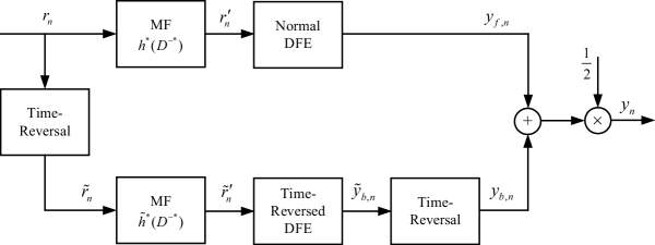
Figure 1: Bidirectional Decision Feedback Equalizer: Infinite Length.

The structure of the BiDFE is shown in Fig. 1. If we assume that the feedback sequence is correct, the outputs of two unbiased DFEs are:

$$Y_{f,n} = X_{n}+V_{f,n}$$ (39)

$$Y_{b,n} = X_{n}+V_{b,n}$$ (40)

where $V_{f,n}$ and $V_{b,n}$ have D-transforms $V_{f}(D)$ and $V_{b}(D)$ as given by (from (30), (31), (35), and (36))

$$V_{f}(D) = \dfrac{N_{0}}{P_{0}-N_{0}}\left(1-\dfrac{1}{g^{*}(D^{-*})}\right)x(D)+\dfrac{P_{x}}{P_{0}-N_{0}}\left(\dfrac{w^{\prime}(D)}{g^{*}(D^{-*})}\right)$$ (41)

$$V_{b}(D) = \dfrac{N_{0}}{P_{0}-N_{0}}\left(1-\dfrac{1}{g(D)}\right)x(D)+\dfrac{P_{x}}{P_{0}-N_{0}}\left(\dfrac{w^{\prime}(D)}{g(D)}\right).$$ (42)

Assuming stationary random processes, we drop time index $n$ for notational simplicity and write: $Y_{f}=X+V_{f}$ and $Y_{b}=X+V_{b}$. From (32) and (37), the variance of $V_{f}$ and $V_{b}$ are also given as:

$$\mathrm{Var}(V_{f})=\mathrm{Var}(V_{b})=\dfrac{P_{x}N_{0}}{P_{0}-N_{0}}.$$

The variables $V_{f}$ and $V_{b}$ are correlated with the correlation coefficient given by

$$\rho \triangleq \dfrac{\mathrm{E}(V_{f}V^{*}_{b})}{\sqrt{\mathrm{Var}(V_{f})\mathrm{Var}(V_{b})}}$$

$$= \dfrac{P_{0}-N_{0}}{P_{x}N_{0}}\mathrm{E}\left[V_{f}(D)V^{*}_{b}(D^{-*})\right]_{0}$$

$$= \dfrac{P_{x}}{N_{0}(P_{0}-N_{0})}\mathrm{E}\left[\left(\dfrac{1}{g^{*}(D^{-*})}\right)^{2}w^{\prime}(D)w^{\prime*}(D^{-*})\right]_{0}$$

$$= \dfrac{P_{0}^{2}}{P_{x}N_{0}(P_{0}-N_{0})}\left[\left\{c(D)\right\}^{2}R_{w^{\prime}w^{\prime}}(D)\right]_{0}$$

$$= \dfrac{P_{0}^{2}}{P_{x}(P_{0}-N_{0})}\left[\left\{c(D)\right\}^{2}R_{hh}(D)\right]_{0}$$ (44)

where $\left[z(D)\right]_{0}=z_{0}$ with $z(D)=\sum_{k}z_{k}D^{k}$. The equality in (IV-C) holds due to the assumption that $X_{n}$ is an i.i.d random variable and the self-interference term is removed from the expression $1-1/g^{*}(D^{-*})$.

Since $\mathrm{Var}(V_{f})=\mathrm{Var}(V_{b})$, the linear MMSE combiner of [7], [14] becomes $Y=\frac{1}{2}\left(Y_{f}+Y_{b}\right)$. Naturally, the MSE and SNR of the unbiased BiDFE are given as

$$\mathrm{MSE}_{UBiDFE} = \dfrac{(1+\mathrm{Re}[\rho])}{2}\mathrm{MSE}_{UDFE}=\dfrac{(1+\mathrm{Re}[\rho])P_{x}N_{0}}{2(P_{0}-N_{0})}$$ (45)

$$\mathrm{SNR}_{UBiDFE} \triangleq \dfrac{P_{x}}{\mathrm{MSE}_{UBiDFE}}=\dfrac{2}{(1+\mathrm{Re}[\rho])}\mathrm{SNR}_{UDFE}=\dfrac{2(P_{0}-N_{0})}{(1+\mathrm{Re}[\rho])N_{0}}$$ (46)

where $\mathrm{Re}[\rho]$ denotes the real part of $\rho$.

Note that the infinite-length normal/time-reversed MMSE-DFE and BiDFE analyzed here do not exploit the a priori information of $X_{n}$. In other words, the feedforward and feedback filters of DFE are derived by assuming $\mathrm{E}(X_{n})=0$ for all $n$, meaning that the calculated SNR performance would reflect the non-turbo ideal-decision BiDFE performance with time-invariant filter taps of Section III-C.

V Derivation of Iterative BiDFE Algorithm

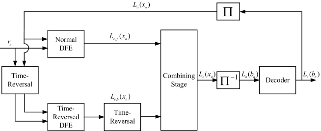
Figure 2: Iterative Equalization Scheme based on BiDFE.

We now discuss an iterative BiDFE algorithm. Iterative equalization schemes based on BiDFE are shown in Fig. 2. Basically, the channel equalizer is a SISO equalizer which employs the normal forward DFE, the time-reversed DFE and an LLR combining block. The received data sequence is equalized in both directions by the two DFEs, and the extrinsic information from two DFEs are combined and passed to the error correction code decoder. We show that a proper combining of the two sets of extrinsic information can suppress error propagation and noise further and generate more reliable extrinsic information for the outer decoder.

V-A Combining Extrinsic Information

Similarly to the finite-length time-varying feedforward and feedback filter of the normal DFE at time index $n$, which are previously defined as $\mathbf{c}_{n}$ in (2) and $\mathbf{d}_{n}$ in (3), we also define the finite-length time-varying feedforward and feedback filter of the time-reversed DFE at time index $n$ as $\mathbf{\tilde{c}}_{n}$ and $\mathbf{\tilde{d}}_{n}$ with the same lengths as $\mathbf{c}_{n}$ and $\mathbf{d}_{n}$ respectively. Note that $\mathbf{\tilde{c}}_{n}$ and $\mathbf{\tilde{d}}_{n}$ are defined in a similar way as (2) and (3) except that the channel convolution matrix $\mathbf{\tilde{H}}$ for the time-reversed channel is given as

$$\mathbf{\tilde{H}}\triangleq\left[{\begin{array}[]{*{20}c}{h_{0}}&{h_{1}}&\cdots&{h_{L_{h}-1}}&0&\cdots&{}\hfil&0\\ 0&{h_{0}}&{h_{1}}&\cdots&{h_{L_{h}-1}}&0&\cdots&0\\ {}\hfil&\ddots&{}\hfil&\ddots&{}\hfil&\ddots&{}\hfil&{}\hfil\\ 0&0&\cdots&0&{h_{0}}&{h_{1}}&\cdots&{h_{L_{h}-1}}\\ \end{array}}\right].$$

The unbiased equalizer output [12] corresponding to the transmitted coded symbol from the the normal (forward) and the time-reversed (backward) DFE can be represented respectively as

$$Y_{f,n} = X_{n}+I_{f,n}+V_{f,n}$$ (47)

$$Y_{b,n} = X_{n}+I_{b,n}+V_{b,n}$$ (48)

where $X_{n}\triangleq x_{n}$, $V_{f,n}\triangleq{v_{f,n}}/{p_{\{n,0\}}}$ and $I_{f,n}\triangleq{i_{f,n}}/{p_{\{n,0\}}}$. Also, $V_{b,n}\triangleq{v_{b,n}}/{\tilde{p}_{\{n,0\}}}$ and $I_{b,n}\triangleq{i_{b,n}}/{\tilde{p}_{\{n,0\}}}$ where $v_{b,n}$ and $i_{b,n}$ are defined similarly to the normal DFE and $\tilde{p}_{\{n,0\}}=\mathbf{\tilde{c}}_{n}^{T}\mathbf{\tilde{s}}$ where ${\mathbf{\tilde{s}}}\triangleq{\mathbf{\tilde{H}}}[\mathbf{0}_{1\times L_{d}},1,\mathbf{0}_{1\times L_{c}}]^{T}$. For notational simplicity, we further drop time index $n$ with an understanding that processing remains identical as $n$ progresses: $Y_{f}=X+I_{f}+V_{f}$ and $Y_{b}=X+I_{b}+V_{b}$.

Now, we discuss the problem of how to combine the extrinsic information from two DFEs. Initially, let us consider two unbiased equalizer outputs, which are corrupted by AWGN, corresponding to the transmitted coded symbol $X$:

$$Y_{f} = X+U_{f}$$

$$Y_{b} = X+U_{b}$$

where the noise $U_{f}$ and $U_{b}$ are assumed to be zero mean Gaussian random variables which are independent of the coded data $X$ but correlated with each other with correlation coefficient $\rho$.

In order to combine the extrinsic information, it is beneficial to whiten the noise $U_{f}$ and $U_{b}$ before combining. The noise correlation matrix $\mathbf{R}$ is defined as

$$\mathbf{R} \triangleq \left[{\begin{array}[]{*{20}c}{\mathrm{Var}(U_{f})}&{\mathrm{E}(U_{f}U_{b})}\\ {\mathrm{E}(U_{f}U_{b})}&{\mathrm{Var}(U_{b})}\\ \end{array}}\right]=\left[{\begin{array}[]{*{20}c}{N_{f}}&{\rho\sqrt{N_{f}N_{b}}}\\ {\rho\sqrt{N_{f}N_{b}}}&{N_{b}}\\ \end{array}}\right]$$ (53)

where $N_{f}\triangleq\mathrm{Var}(U_{f})$ and $N_{b}\triangleq\mathrm{Var}(U_{b})$. Then, the eigenvalues of the noise correlation matrix, $\lambda_{1}$ and $\lambda_{2}$, with their corresponding normalized eigenvectors $\mathbf{g}_{1}$ and $\mathbf{g}_{2}$ are given by

$$\lambda_{1}=\dfrac{(N_{f}+N_{b})+\sqrt{(N_{f}-N_{b})^{2}+4\rho^{2}N_{f}N_{b}}}{2}$$

$$\lambda_{2}=\dfrac{(N_{f}+N_{b})-\sqrt{(N_{f}-N_{b})^{2}+4\rho^{2}N_{f}N_{b}}}{2}$$

$$\mathbf{g}_{1}=\dfrac{1}{\sqrt{g_{11}^{2}+g_{21}^{2}}}\left[{\begin{array}[]{*{20}c}{g_{11}}\\ {g_{21}}\\ \end{array}}\right],\>\mathbf{g}_{2}=\dfrac{1}{\sqrt{g_{12}^{2}+g_{22}^{2}}}\left[{\begin{array}[]{*{20}c}{g_{12}}\\ {g_{22}}\\ \end{array}}\right]$$ (58)

where $g_{11}=\frac{1}{2}\Big{[}(N_{f}-N_{b})+\sqrt{(N_{f}-N_{b})^{2}+4\rho^{2}N_{f}N_{b}}\Big{]}$, $g_{12}=\frac{1}{2}\Big{[}(N_{f}-N_{b})-\sqrt{(N_{f}-N_{b})^{2}+4\rho^{2}N_{f}N_{b}}\Big{]}$, and $g_{21}=g_{22}=\rho\sqrt{N_{f}N_{b}}$. It is easy to see that the noise correlation matrix $\mathbf{R}$ is non-singular unless $\rho=\pm 1$. If $\mathbf{R}$ is non-singular, $\mathbf{R}$ can be expanded as $\mathbf{R}=\mathbf{G}\mathbf{\Lambda}\mathbf{G}^{-1}$ where $\mathbf{G}\triangleq\left[\mathbf{g}_{1}\>\mathbf{g}_{2}\right]$ and $\mathbf{\Lambda}\triangleq\mathrm{Diag}(\lambda_{1},\lambda_{2})$. Since $\mathbf{G}$ is a unitary matrix, the noise whitening matrix is $\mathbf{A}\triangleq\left[\mathbf{a}_{1}\>\mathbf{a}_{2}\right]=\mathbf{G}^{-1}=\mathbf{G}^{T}$ where $\mathbf{a}_{1}\triangleq\left[a_{11}\>a_{21}\right]^{T}$ and $\mathbf{a}_{2}\triangleq\left[a_{12}\>a_{22}\right]^{T}$. So, given the equalized output vector $\mathbf{Y}\triangleq[Y_{f},Y_{b}]^{T}$, the whitened vector is $\mathbf{Y}^{\prime}\triangleq[Y^{\prime}_{f},Y^{\prime}_{b}]^{T}=\mathbf{A}\mathbf{Y}$ with the new noise correlation matrix $\mathbf{R}^{\prime}=\mathbf{A}\mathbf{R}\mathbf{A}^{T}=\mathbf{\Lambda}$. Finally, the extrinsic information of $X$ can be expressed as

$$L_{e}(X) = \ln\dfrac{\mathrm{Pr}(Y_{f},Y_{b}\mid X=+1)}{\mathrm{Pr}(Y_{f},Y_{b}\mid X=-1)}$$ (59)

$$= \ln\dfrac{\mathrm{Pr}(Y^{\prime}_{f},Y^{\prime}_{b}\mid X=+1)}{\mathrm{Pr}(Y^{\prime}_{f},Y^{\prime}_{b}\mid X=-1)}$$

$$= \ln\dfrac{\mathrm{Pr}(Y^{\prime}_{f}\mid X=+1)}{\mathrm{Pr}(Y^{\prime}_{f}\mid X=-1)}+\ln\dfrac{\mathrm{Pr}(Y^{\prime}_{b}\mid X=+1)}{\mathrm{Pr}(Y^{\prime}_{b}\mid X=-1)}$$

$$= \dfrac{2(a_{11}+a_{12})Y^{\prime}_{f}}{\lambda_{1}}+\dfrac{2(a_{21}+a_{22})Y^{\prime}_{b}}{\lambda_{2}}$$

$$= \dfrac{2\left(N_{b}-\rho\sqrt{N_{f}N_{b}}\right)Y_{f}}{\left(1-\rho^{2}\right)N_{f}N_{b}}+\dfrac{2\left(N_{f}-\rho\sqrt{N_{f}N_{b}}\right)Y_{b}}{\left(1-\rho^{2}\right)N_{f}N_{b}}$$

$$= \dfrac{\left(N_{b}-\rho\sqrt{N_{f}N_{b}}\right)}{\left(1-\rho^{2}\right)N_{b}}L_{e,f}(X)+\dfrac{\left(N_{f}-\rho\sqrt{N_{f}N_{b}}\right)}{\left(1-\rho^{2}\right)N_{f}}L_{e,b}(X).$$

For the singular noise correlation matrix $\mathbf{R}$ (i.e., $\rho=+1$), $N_{f}=N_{b}=N$ and $Y_{f}=Y_{b}=Y$ so that $L_{e,f}(X)=L_{e,b}(X)$. Consequently, the extrinsic information of $X$ becomes $L_{e}(X)=2Y/N=(L_{e,f}(X)+L_{e,b}(X))/2$. Note that the mean combiner of [9], $L_{e}(X)=(L_{e,f}(X)+L_{e,b}(X))/2$, can be considered as the proposed combiner with $\rho=+1$. If $\rho=-1$, $U_{f}=-U_{b}$ and we can cancel out the noise perfectly by averaging the outputs: $(Y_{f}+Y_{b})/2$. The extrinsic information of $X$ in this case is $L_{e}(X)=+\infty$ when $(Y_{f}+Y_{b})/2\geq 0$ while $L_{e}(X)=-\infty$ when $(Y_{f}+Y_{b})/2<0$.

V-B Reducing the Combiner Sensitivity to the Estimation Error

Let us consider the effect of errors in estimating $\rho$ on extrinsic information. Write $\hat{\rho}=\rho+\varepsilon$ where $\varepsilon$ is the estimation error. Then, the sensitivity of the combiner in (59) to the estimation error can be defined as

$$\mathrm{S}(\rho) \triangleq \left|\dfrac{\partial L_{e}(X)}{\partial\rho}\right|$$

$$= \bigg{|}\dfrac{\left(2\rho N_{b}-(1+\rho^{2})\sqrt{N_{f}N_{b}}\right)}{\left(1-\rho^{2}\right)^{2}N_{b}}L_{e,f}(X)+\dfrac{\left(2\rho N_{f}-(1+\rho^{2})\sqrt{N_{f}N_{b}}\right)}{\left(1-\rho^{2}\right)^{2}N_{f}}L_{e,b}(X)\bigg{|}$$

which approaches infinity as $\rho\rightarrow\pm 1$. This means that the combiner of (59) is unfortunately very sensitive to the correlation estimator error, as the magnitude of the correlation becomes large.

The sensitivity of the combiner can be reduced if we assume that the variance of $U_{f}$ and $U_{b}$ are the same, i.e., $N=N_{f}=N_{b}=(N_{f}+N_{b})/2$. This assumption is reasonable when the same feedforward and feedback filter length is used in both DFEs. Then, from (59), the combined extrinsic information of $X$ for non-singular $\mathbf{R}$ is simply given as

$$L_{e}(X)=\dfrac{1}{(1+\rho)}\Big{(}L_{e,f}(X)+L_{e,b}(X)\Big{)}$$ (60)

with the sensitivity to the correlation estimation error

$$\mathrm{S}(\rho)=\left|\dfrac{1}{(1+\rho)^{2}}\Big{(}L_{e,f}(X)+L_{e,b}(X)\Big{)}\right|.$$

Although the sensitivity of this combiner to the estimation error also goes to infinity as $\rho\rightarrow-1$, it shows more robustness as $\rho\rightarrow+1$ since $\lim_{\rho\rightarrow+1}\mathrm{S}(\rho)=\left|(L_{e,f}(X)+L_{e,b}(X))/4\right|$.

V-C Application to the BiDFE Algorithm

In this paper, although the composite noise $I_{f,n}+V_{f,n}$ and $I_{b,n}+V_{b,n}$ are not Gaussian, we exploit the combiner of (60) in order to produce the combined extrinsic information to be passed to the convolutional decoder. The noise correlation coefficient between $I_{f,n}+V_{f,n}$ and $I_{b,n}+V_{b,n}$ is naturally defined as

$$\rho_{n} \triangleq \dfrac{\mathrm{E}\left\{\left(I_{f,n}-\mathrm{E}(I_{f,n})+V_{f,n}\right)\left(I_{b,n}-\mathrm{E}(I_{b,n})+V_{b,n}\right)\right\}}{\sqrt{\left(\mathrm{Var}(I_{f,n})+\mathrm{Var}(V_{f,n})\right)\left(\mathrm{Var}(I_{b,n})+\mathrm{Var}(V_{b,n})\right)}}.$$ (61)

Unfortunately, it is difficult to compute the correlation coefficient analytically in the presence of decision feedback errors. However, assuming that the noise is stationary, we have $\rho_{n}=\rho$ and the correlation coefficient can be estimated through time-averaging:

$$\hat{\rho} = \dfrac{\sum\left\{(Y_{f,n}-\hat{X}_{f,n}-\mathrm{E}(I_{f,n}))(Y_{b,n}-\hat{X}_{b,n}-\mathrm{E}(I_{b,n}))\right\}}{\sqrt{\sum(Y_{f,n}-\hat{X}_{f,n}-\mathrm{E}(I_{f,n}))^{2}}\sqrt{\sum(Y_{b,n}-\hat{X}_{b,n}-\mathrm{E}(I_{b,n}))^{2}}}$$ (62)

where the summations are over some reasonably large finite window. Note that the hard decisions for the transmitted symbols in normal and time-reversed DFEs might be different; in estimating the correlation coefficient, we only consider those noise samples for which $\hat{X}_{f,n}$ and $\hat{X}_{b,n}$ are identical.

Let us summarize our LLR combining method: 1) The extrinsic information $L_{e,f}(X_{n})$ and $L_{e,b}(X_{n})$ for $n=1,2,\ldots,L$ are acquired according to (22) in the normal and time-reversed MMSE-DFE settings. 2) Estimate the noise correlation coefficient, $\hat{\rho}$, between $I_{f,n}+V_{f,n}$ and $I_{b,n}+V_{b,n}$ by (62). 3) Generate the combined extrinsic information $L_{e}(X_{n})$ according to (60) with $\rho_{n}=\hat{\rho}$.

V-D Correlation Analysis under Ideal Feedback

We provide correlation analysis in the following. The analysis will allow validation of (62) in different scenarios. The observation of how the simulated correlation coefficient (62) converges to the analytically computed one under the assumptions of ideal feedback and perfect a priori information will also provide useful insights into the iterative behaviour of the proposed turbo BiDFE.

First of all, the noise variance of $V_{f,n}$ and $V_{b,n}$ from the time-varying filters are:

$$\mathrm{Var}(V_{f,n}) = (1-\mathbf{s}^{T}\mathbf{c}_{n})/\mathbf{c}_{n}^{T}\mathbf{s}$$

$$\mathrm{Var}(V_{b,n}) = (1-\mathbf{\tilde{s}}^{T}\mathbf{\tilde{c}}_{n})/\mathbf{\tilde{c}}_{n}^{T}\mathbf{\tilde{s}}.$$

When we assume ideal decision feedback, $\mathrm{Pr}(I_{f}=0)=\mathrm{Pr}(I_{b}=0)=1$ so that $I_{f,n}=I_{b,n}=0$, the noise correlation coefficient $\rho_{n}$ between $V_{f,n}$ and $V_{b,n}$ becomes

$$\rho_{n} \triangleq \dfrac{\mathrm{E}(V_{f,n}V_{b,n})}{\sqrt{\mathrm{Var}(V_{f,n})\mathrm{Var}(V_{b,n})}}$$

$$= \dfrac{\mathrm{E}\left[\left\{\dfrac{1}{p_{\{n,0\}}}\sum\limits_{j=0}^{L_{c}}c_{\{n,j\}}w_{n+j}\right\}\left\{\dfrac{1}{\tilde{p}_{\{n,0\}}}\sum\limits_{k=0}^{L_{c}}\tilde{c}_{\{n,k\}}w_{n-k+L_{h}-1}\right\}\right]}{\sqrt{(1-\mathbf{s}^{T}\mathbf{c}_{n})/\mathbf{c}_{n}^{T}\mathbf{s}}\sqrt{(1-\mathbf{\tilde{s}}^{T}\mathbf{\tilde{c}}_{n})/\mathbf{\tilde{c}}_{n}^{T}\mathbf{\tilde{s}}}}$$

$$= \dfrac{\sum\limits_{j=0}^{L_{c}}\sum\limits_{k=0}^{L_{c}}c_{\{n,j\}}\tilde{c}_{\{n,k\}}\mathrm{E}\left[w_{n+j}w_{n-k+L_{h}-1}\right]}{\sqrt{\mathbf{c}_{n}^{T}\mathbf{s}(1-\mathbf{s}^{T}\mathbf{c}_{n})}\sqrt{\mathbf{\tilde{c}}_{n}^{T}\mathbf{\tilde{s}}(1-\mathbf{\tilde{s}}^{T}\mathbf{\tilde{c}}_{n})}}$$

$$= N_{0}\left(\dfrac{\sum\limits_{j=0}^{L_{c}}\sum\limits_{k=0}^{L_{c}}c_{\{n,j\}}\tilde{c}_{\{n,k\}}\delta(j+k+1-L_{h})}{\sqrt{\mathbf{c}_{n}^{T}\mathbf{s}(1-\mathbf{s}^{T}\mathbf{c}_{n})}\sqrt{\mathbf{\tilde{c}}_{n}^{T}\mathbf{\tilde{s}}(1-\mathbf{\tilde{s}}^{T}\mathbf{\tilde{c}}_{n})}}\right)$$ (64)

where $\delta(t)$ is defined as: if $t=0$, $\delta(t)=1$; otherwise, $\delta(t)=0$. The equality in (V-D) holds because $X_{n}$ is an i.i.d random variable.

If the time-invariant filters are used instead of the time-varying filters, the variances of $V_{f,n}$ and $V_{b,n}$ become

$$\mathrm{Var}(V_{f,n}) = \mathbf{c}^{T}\left(\mathbf{H}\mathbf{\Sigma}_{n}\mathbf{H}^{T}-z_{n}\mathbf{s}\mathbf{s}^{T}+{N_{0}\mathbf{I}}\right)\mathbf{c}/\left(\mathbf{c}^{T}\mathbf{s}\right)^{2}$$

$$\mathrm{Var}(V_{b,n}) = \mathbf{\tilde{c}}^{T}\left(\mathbf{\tilde{H}}\mathbf{\tilde{\Sigma}}_{n}\mathbf{\tilde{H}}^{T}-z_{n}\mathbf{\tilde{s}}\mathbf{\tilde{s}}^{T}+{N_{0}\mathbf{I}}\right)\mathbf{\tilde{c}}/\left(\mathbf{\tilde{c}}^{T}\mathbf{\tilde{s}}\right)^{2}.$$

Then, the noise correlation coefficient can be also obtained as

$$\rho_{n} = N_{0}\left(\dfrac{\sum\limits_{j=0}^{L_{c}}\sum\limits_{k=0}^{L_{c}}c_{j}\tilde{c}_{k}\delta(j+k+1-L_{h})}{\sqrt{\mathbf{c}^{T}\left(\mathbf{H}\mathbf{\Sigma}_{n}\mathbf{H}^{T}-z_{n}\mathbf{s}\mathbf{s}^{T}+{N_{0}\mathbf{I}}\right)\mathbf{c}}\sqrt{\mathbf{\tilde{c}}^{T}(\mathbf{\tilde{H}}\mathbf{\tilde{\Sigma}}_{n}\mathbf{\tilde{H}}^{T}-z_{n}\mathbf{\tilde{s}}\mathbf{\tilde{s}}^{T}+{N_{0}\mathbf{I}})\mathbf{\tilde{c}}}}\right).$$ (65)

Now, let us consider some special cases.

V-D1 No A Priori Information

When no a priori information is available, i.e., $\mathrm{E}(X_{n})=0$ for all $n$, the feedforward and feedback filters are the same as the time-invariant filters and the noise variances are stationary:

$$\mathrm{Var}(V_{f,n}) = \mathrm{Var}(V_{f})=(1-\mathbf{s}^{T}\mathbf{c})/\mathbf{c}^{T}\mathbf{s}$$

$$\mathrm{Var}(V_{b,n}) = \mathrm{Var}(V_{b})=(1-\mathbf{\tilde{s}}^{T}\mathbf{\tilde{c}})/\mathbf{\tilde{c}}^{T}\mathbf{\tilde{s}}.$$

Therefore, the noise correlation coefficient is given by

$$\rho_{n} = \rho=N_{0}\left(\dfrac{\sum\limits_{j=0}^{L_{c}}\sum\limits_{k=0}^{L_{c}}c_{j}\tilde{c}_{k}\delta(j+k+1-L_{h})}{\sqrt{\mathbf{c}^{T}\mathbf{s}(1-\mathbf{s}^{T}\mathbf{c})}\sqrt{\mathbf{\tilde{c}}^{T}\mathbf{\tilde{s}}(1-\mathbf{\tilde{s}}^{T}\mathbf{\tilde{c}})}}\right).$$ (66)

We observed that the noise correlation coefficient of the infinite-length BiDFE in (44) is almost identical to that of the finite-length BiDFE in (66) when $L_{c}$ is chosen to be long enough.

V-D2 Time-varying Filters with Perfect A Priori Information

When several iterations are performed at high SNRs in turbo equalization, the perfect a priori information could be available, i.e., $\mathrm{E}(X_{n})=X_{n}$ for all $n$. When $\mathrm{E}(X_{n})=X_{n}$ for all $n$, the feedforward filters $\mathbf{c}_{n}$ and $\mathbf{\tilde{c}}_{n}$ of two DFEs become the normalized matched filters corresponding to the forward and reverse channel impulse responses:

$$\mathbf{c}_{n} = A\left[h_{0},h_{1},\ldots,h_{L_{h}-1},\mathbf{0}_{1\times L_{c}-L_{h}+1}\right]^{T}$$

$$\mathbf{\tilde{c}}_{n} = A\left[h_{L_{h}-1},h_{L_{h}-2},\ldots,h_{0},\mathbf{0}_{1\times L_{c}-L_{h}+1}\right]^{T}$$

where $A$ is a real-valued constant depending on SNR, i.e., $A\triangleq 1/(N_{0}+\sum_{k=0}^{L_{h}-1}|h_{k}|^{2})$. Moreover, since the first terms of $V_{f,n}$ and $V_{b,n}$ disappear, the noise variances are simply:

$$\mathrm{Var}(V_{f,n}) = \mathrm{Var}(V_{f})=N_{0}\mathbf{c}_{n}^{T}\mathbf{c}_{n}/(\mathbf{c}_{n}^{T}\mathbf{s})^{2}=\dfrac{N_{0}A^{2}}{(\mathbf{c}_{n}^{T}\mathbf{s})^{2}}\sum_{k=0}^{L_{h}-1}|h_{k}|^{2}$$

$$\mathrm{Var}(V_{b,n}) = \mathrm{Var}(V_{b})=N_{0}\mathbf{\tilde{c}}_{n}^{T}\mathbf{\tilde{c}}_{n}/(\mathbf{\tilde{c}}_{n}^{T}\mathbf{\tilde{s}})^{2}=\dfrac{N_{0}A^{2}}{(\mathbf{\tilde{c}}_{n}^{T}\mathbf{\tilde{s}})^{2}}\sum_{k=0}^{L_{h}-1}|h_{k}|^{2}.$$

Accordingly, the noise correlation coefficient is

$$\rho_{n}=\rho=1.$$ (67)

Note that the noise correlation coefficient $\rho$ with perfect a priori information converges to 1 regardless of the SNR value. As will be shown shortly, the measured correlation coefficient using simulated turbo BiDFE outputs indeed approaches 1, as turbo iteration progresses. This indicates that both assumptions - ideal decision feedback and perfect a priori information - are reasonable.

V-D3 Time-invariant Filters with Perfect A Priori Information

When the time-invariant filters are used with perfect a priori information, the time-invariant DFEs yield the noise variances as

$$\mathrm{Var}(V_{f,n}) = \mathrm{Var}(V_{f})=N_{0}\mathbf{c}^{T}\mathbf{c}/(\mathbf{c}^{T}\mathbf{s})^{2}$$

$$\mathrm{Var}(V_{b,n}) = \mathrm{Var}(V_{b})=N_{0}\mathbf{\tilde{c}}^{T}\mathbf{\tilde{c}}/(\mathbf{\tilde{c}}^{T}\mathbf{\tilde{s}})^{2}.$$

The noise correlation coefficient is also simply given by

$$\rho_{n}=\rho=\dfrac{\sum\limits_{j=0}^{L_{c}}\sum\limits_{k=0}^{L_{c}}c_{j}\tilde{c}_{k}\delta(j+k+1-L_{h})}{\sqrt{\mathbf{c}^{T}\mathbf{c}}\sqrt{\mathbf{\tilde{c}}^{T}\mathbf{\tilde{c}}}}.$$ (68)

As will be discussed in the next section, in the simulation of turbo BiDFE with time-invariant taps it is observed that the BiDFE output correlation does indeed converge to (68), indicating again that the assumptions of error-free decisions and perfect a priori information are reasonable.

VI Simulation Results

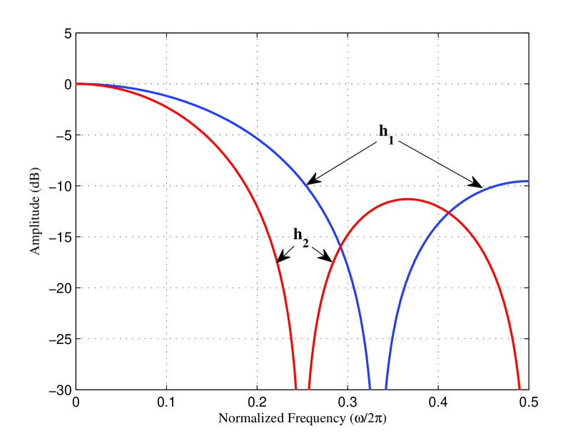
Figure 3: Frequency Magnitude Response of the ISI Channels: $\mathbf{h_{1}}=(1/\sqrt{19})[1\quad 2\quad 3\quad 2\quad 1]^{T}$, $\mathbf{h_{2}}=(1/\sqrt{44})[1\quad 2\quad 3\quad 4\quad 3\quad 2\quad 1]^{T}$.

In this section, simulation results of several iterative equalization schemes are presented. The transmitted symbols are encoded with a recursive rate-$1/2$ convolutional code encoder with parity generator $(1+D^{2})/(1+D+D^{2})$ with $2^{11}$ message bits and are modulated by binary phase-shift keying (BPSK) so that $x_{n}\in\{\pm 1\}$. We also assume that the noise is AWGN, and the noise variance and the channel information are perfectly known to the receiver. The ISI channels with impulse responses $\mathbf{h_{1}}=(1/\sqrt{19})[1\quad 2\quad 3\quad 2\quad 1]^{T}$ and $\mathbf{h_{2}}=(1/\sqrt{44})[1\quad 2\quad 3\quad 4\quad 3\quad 2\quad 1]^{T}$ investigated in [3] and [10] are used for evaluating the performance of the iterative equalizers. These channels are considered very severe ISI channels as the channel spectra possess nulls over the Nyquist band, as shown in Fig. 3. Finally, the decoder is implemented using the BCJR algorithm. Only the SISO equalizer changes from one scheme to another. The MMSE-DFE with 17 feedforward taps and 4 feedback taps is used for both the normal and the time-reversed DFEs on $\mathbf{h_{1}}$ while MMSE-DFE with 21 feedforward taps and 6 feedback taps is used on $\mathbf{h_{2}}$. Finally, the linear MMSE equalizer uses 21 taps for $\mathbf{h_{1}}$ and 27 taps for $\mathbf{h_{2}}$.

Six different equalizer types are simulated in this work. The notation “TV-” denotes equalizers with time-varying filters while “TIV-” indicates those with time-invariant filters. For instance, “TV-LE” in the legend indicates the linear MMSE equalizer with a time-varying filter. The “Proposed DFE” uses the proposed LLR mapping of (22) while “DFE” uses the conventional LLR mapping (as used in [3]) The “Proposed BiDFE” is the iterative BiDFE algorithm which is described in Section V. In other words, “Proposed BiDFE” uses the the proposed LLR generation for both normal and time-reversed DFEs along with the proposed extrinsic information combiner of (60) in conjunction with the noise correlation coefficient of (62). The “BiDFE (mean combiner)” is the iterative BiDFE algorithm with the conventional LLR mapping and the mean combiner, $L_{e}(X)=(L_{e,f}(X)+L_{e,b}(X))/2$ (of [9]), simulated for performance comparison purposes. Finally, “MAP” is the optimal equalizer implemented via the BCJR algorithm.

A thorough comparison is given in [3] on the required complexity levels of the SISO-LE, SISO-DFE and the MAP equalizers. The exact level of implementation complexity is hard to assess as it depends highly on specific VLSI architecture details. Roughly speaking, however, it is safe to say that the number of multiplications and additions increases as an exponential function of the channel memory length for the MAP equalizer whereas the number of the same operations is a quadratic function of both the channel memory length and the filter length for the TV-LE and the TV-DFE, as shown in [3]. The number of operations, on the other hand, increases only linearly for the TIV-LE and the TIV-DFE [3]. The BiDFE equalizers, including the proposed BiDFE methods, require roughly twice as many operations as the DFE counterparts, due to the presence of the time-reversed filter components. Most notably, while the complexity of the proposed BiDFE with time-invariant filters is considerably lower than that of the MAP equalizer as well as the TV-LE, the performance is significantly better than the TV-LE.

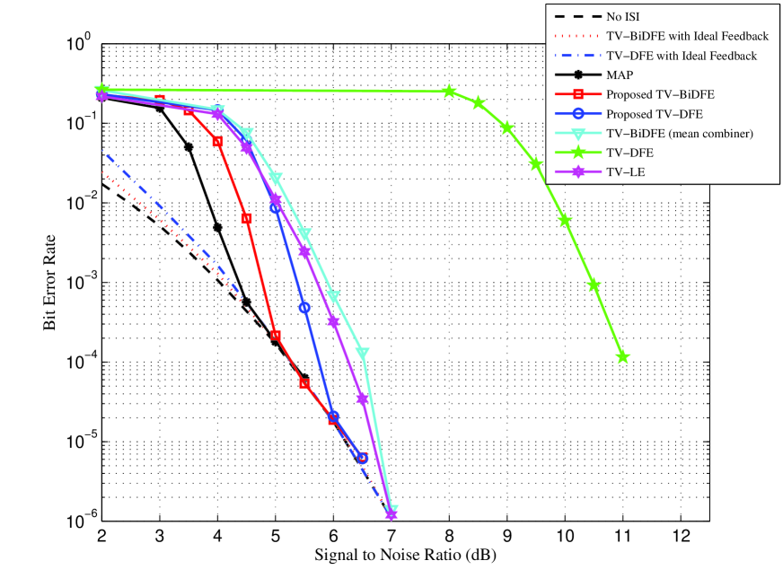
Figure 4: BER Curve on the Channel $\mathbf{h_{1}}$ after 20 Iterations with Time-varying Filters.

Fig. 4 shows the performance of several turbo equalizers with time-varying filters after 20 iterations. TV-DFE with the conventional LLR mapping shows poor performance but once the proposed LLR generations are used (“Proposed TV-DFE”), the DFE performance becomes clearly better than the TV-LE method of [3], except at very high SNRs where all schemes other than the conventional DFE perform comparably. The “Proposed TV-BiDFE” is considerably better than the TV-BiDFE based on the mean combiner, approaching the performance of the MAP scheme.

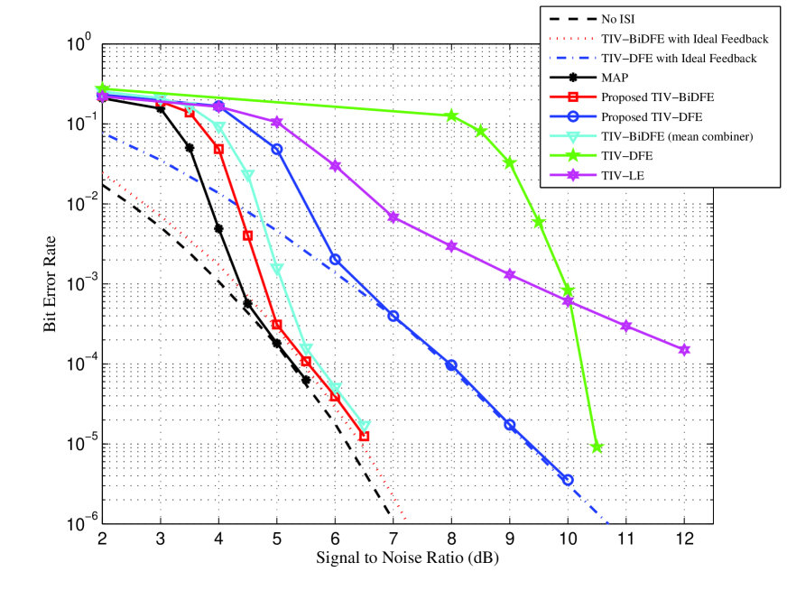
Figure 5: BER Curve on the Channel $\mathbf{h_{1}}$ after 20 iterations with Time-invariant Filters.

Fig. 5 shows the BER performance of time-invariant-filter-based turbo equalizers. As the figure indicates, the “Proposed TIV-DFE” also shows superior performance to the “TIV-DFE”. The performance of “Proposed TIV-BiDFE” is very close to the performance of the MAP equalizer while requiring low computational complexity based on the use of time-invariant filters. Also notice that both “Proposed TIV-DFE” and “Proposed TIV-BiDFE” achieve decision-error-free performance at low BERs, indicating the error propagation effect has been nearly eliminated using the proposed LLR generation method. It is noteworthy that the proposed BiDFE algorithm still provides near-optimal performance even with the time-invariant filter taps. While the TIV-BiDFE based on the existing mean combiner appears to perform almost as well, the EXIT chart analysis to be discussed below indicate that with a smaller number of turbo iterations, its performance is distinctly inferior to the proposed TIV-BiDFE based on the new combining method.

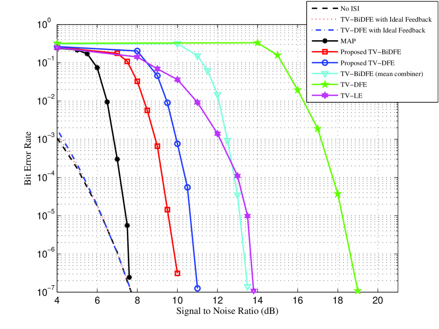
Figure 6: BER Curve on the Channel $\mathbf{h_{2}}$ after 20 Iterations with Time-varying Filters.

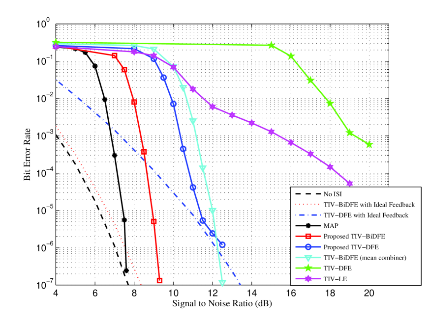
Figure 7: BER Curve on the Channel $\mathbf{h_{2}}$ after 20 iterations with Time-invariant Filters.

Figs. 6 and 7 show a similar set of simulation results now applied to the more severe ISI channel $\mathbf{h_{2}}$. While all DFE-based schemes lag clearly behind the BCJR-based scheme at the error rates simulated, the proposed BiDFE scheme in both the time-varying and time-invariant filter cases outperform the LE scheme by a significant margin. In fact, in this severe channel the BER curve of the LE scheme, even with time-varying filters, appears to diverge considerably from the ideal no-ISI curve. Overall, the proposed BiDFE based on time-invariant filter taps offer excellent performance-complexity trade-off.

The noise correlation in one block of coded data bits is described in Fig. 8, at different iteration numbers at a 6 dB SNR on $\mathbf{h_{1}}$. The correlation coefficient of “Proposed TV-BiDFE” goes to 1 as the number of iterations increases because the a priori information from the decoder becomes reliable, and the time-varying filters in the normal and the time-reversed DFEs produce essentially the same equalized output sequences. This phenomenon of Fig. 8 validates (67). On the other hand, the correlation coefficient of “Proposed TIV-BiDFE” actually decreases as the number of iterations increases, and the noise correlation coefficient converges to that of “TIV-BiDFE with Ideal Feedback” or the correlation coefficient of (68). This is because the decision feedback errors disappear and the perfect a priori information is available from decoder. Note that the filter coefficients in both DFEs do not change with the a priori information.

In general, it is quite difficult to analyse the iterative equalization and decoding schemes. We rely on the oft-used extrinsic information transfer (EXIT) chart of [15] to develop insights into the convergence behaviour of the turbo equalizers. The EXIT chart is a diagram demonstrating the mutual information (MI) transfer characteristics of the two constituent modules which exchange soft information. In the EXIT charts, the behavior of the channel equalizer is described with its input and output on the horizontal and vertical axis, respectively, while the behavior of the decoder is described in opposite way. The pair of EXIT chart curves typically defines a path for the MI trajectory to move up during iterative processing of soft information. The number of stairs that a given MI trajectory takes to reach the highest value indicates the necessary number of iterations toward convergence.

Figs. 9 and 11 show the EXIT chart corresponding to time-varying-filter-based equalizers for $\mathbf{h_{1}}$ at a 6 dB SNR and $\mathbf{h_{2}}$ at a 10 dB SNR while Figs. 10 and 12 show the similar EXIT charts for time-invariant-filter-based schemes. Although not shown here to avoid excessive cluttering, the trajectories of “TV-DFE” and “TIV-DFE” move up for the first couple of iterations, but then quickly fizzle out due to the inadequate extrinsic LLR generations that cannot handle error propagation. However, the trajectories of “Proposed TV-DFE” and “Proposed TIV-DFE” keep moving up as the number of iterations increases, clearly indicating the advantage and effectiveness of the proposed LLR generation method. However, the trajectory of “Proposed TIV-DFE” at 6 dB or 10 dB does not reach the maximum possible value since the filters do not fully exploit the a priori information from the decoder. The trajectories of the “Proposed TV-BiDFE” and “Proposed TIV-BiDFE” indicate that these schemes move from 0 bit of mutual information to 1 bit with a less number of iteration runs than “Proposed TV-DFE”, “Proposed TIV-DFE”, “TV-LE”, or “TIV-LE”.

We notice, however, that the proposed BiDFE scheme requires more iterations in achieving the full performance, relative to the MAP equalizer (whose trajectory is not shown to avoid cluttering). Nevertheless, the proposed BiDFE method offers a reasonable tradeoff among complexity, performance, and latency.

Finally, Fig. 13 shows the SNR comparison at the output of the unbiased DFE and BiDFE assuming ideal feedback on the channel $\mathbf{h_{1}}$ when the a priori information is not available. As the figure shows, the output SNR of BiDFE is considerably higher than the output SNR of DFE but with a certain gap to the matched filter bound (MFB).

VII Conclusion

In this paper, we proposed new SISO DFE and BiDFE structures well-suited to turbo equalization. The proposed LLR generation designed to reduce error propagation indeed provides decision-error-free performance in the DFE in turbo equalizer setting. When further employing an LLR combining method that estimates the correlation between the forward and backward DFE outputs and whitens them, the resulting performance is remarkably good given the simple structure of the BiDFE, relative to that of the BCJR equalizer. The proposed LLR generation and combining methods remain effective even when a time-invariance constraint is imposed on the feedforward and feedback filters of the DFEs. Overall, the proposed BiDFE method based on time-invariant filter taps provides the excellent performance-complexity tradeoff for severe ISI channels where the linear SISO equalizer fails to operate adequately.

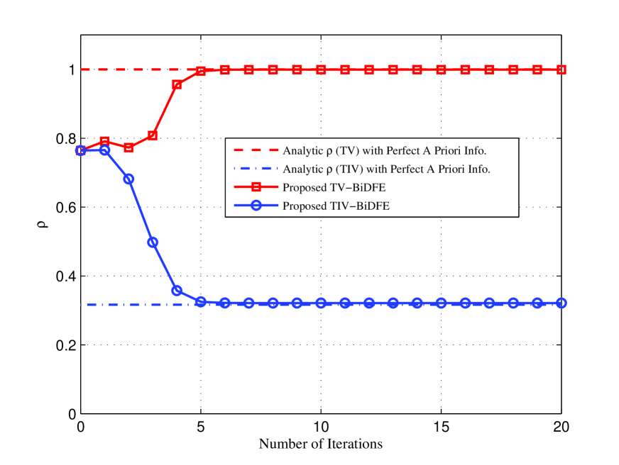
Figure 8: Noise Correlation of “Proposed BiDFE” on the Channel $\mathbf{h_{1}}$.

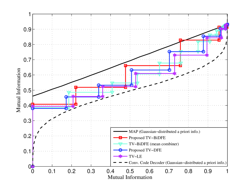
Figure 9: EXIT Chart on the Channel $\mathbf{h_{1}}$ at a 6 dB with Time-varying Filters.

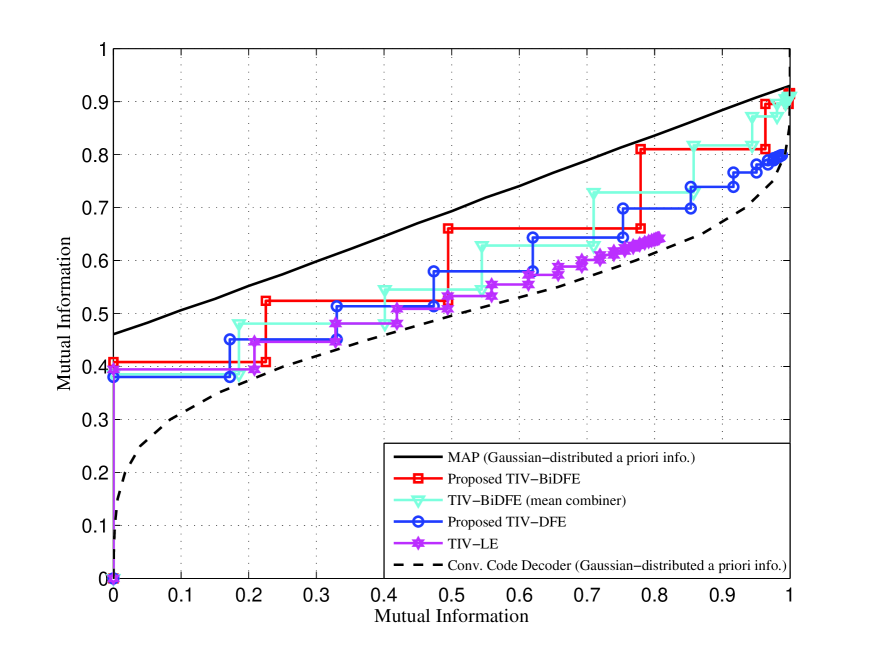
Figure 10: EXIT Chart on the Channel $\mathbf{h_{1}}$ at a 6 dB with Time-invariant Filters.

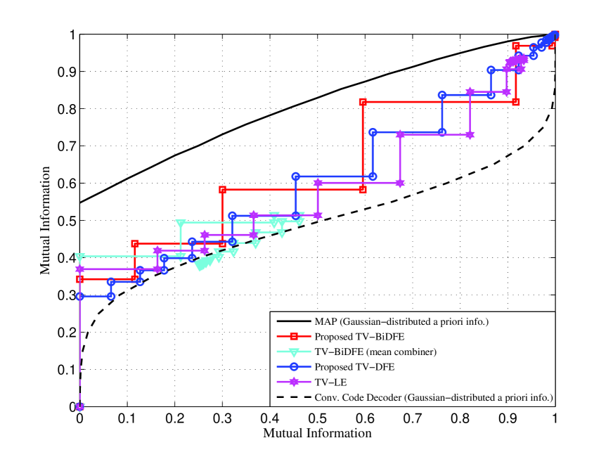
Figure 11: EXIT Chart on the Channel $\mathbf{h_{2}}$ at a 10 dB with Time-varying Filters.

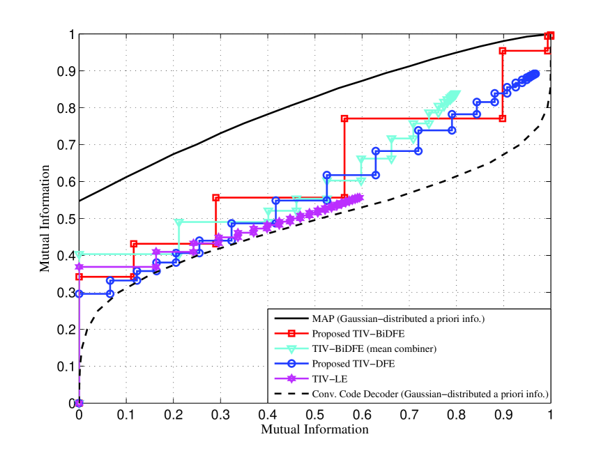
Figure 12: EXIT Chart on the Channel $\mathbf{h_{2}}$ at a 10 dB with Time-invariant Filters.

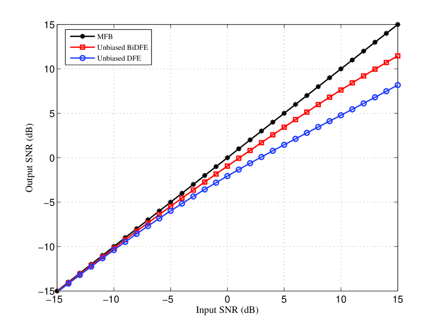
Figure 13: SNR plot on the Channel $\mathbf{h_{1}}$.

References

- [1] C. Douillard, M. Jezequel, C. Berrou, A. Picart, P. Didier, and A. Glavieux, “Iterative correction of intersymbol interference: Turbo equalization,” European Trans. Telecommun., vol. 6, no. 5, pp. 507-511, Sep.-Oct. 1995.
- [2] L. Bahl, J. Cocke, F. Jelinek, and J. Raviv, “Optimal Decoding of Linear Codes for Minimizing Symbol Error Rate,” IEEE Trans. Information Theory, vol. IT-20, pp. 284-287, Mar. 1974.
- [3] M. Tüchler, R. Kötter, and A. Singer, “Turbo equalization: principles and new results,” IEEE Trans. Signal Processing, vol. 50, no. 5, pp. 754-767, May 2002.
- [4] A. Fertner, “Improvement of bit-error-rate in decision feedback equalizer by preventing decision-error propagation,” IEEE Trans. Signal Processing, vol. 46, no. 7, pp. 1872-1877, Jul. 1998.
- [5] S. Ariyavisitakul and Y. Li, “Joint coding and decision feedback equalization for broadband wireless channels,” IEEE Trans. Selected Areas in Communications, vol. 16, no. 9, pp. 1670-1678, Dec. 1998.
- [6] R. R. Lopes and J. R. Barry, “The Soft-Feedback Equalization for Turbo Equalization of Highly Dispersive Channels,” IEEE Trans. Communications, vol. 54, no. 5, pp. 783-788, May 2006.
- [7] J. Balakrishnan and C. R. Johnson, Jr., “Bidirectional Decision Feedback Equalizer: Infinite Length Results,” In Proc. Asilomar Conf. on Signals, Systems, and Computers, Pacific Grove, CA, Nov. 2001, pp. 1450-1454.
- [8] J. Nelson, A. Singer, U. Madhow, and C. McGahey, “BAD: bidirectional arbitrated decision-feedback equalization,” IEEE Trans. Communications, vol. 53, no. 2, pp. 214-218, Feb. 2005.
- [9] J. Jiang, C. He, E. M. Kurtas, and K. R. Narayanan, “Performance of soft feedback equalization over magnetic recording channels,” In Proc. Intermag, San Diego, CA, May 2006, pp. 795.
- [10] J. Moon and F. R. Rad, “Turbo Equalization via Constrained-Delay APP Estimation With Decision Feedback,” IEEE Trans. Communications, vol. 53, no. 12, pp. 2102-2113, Dec. 2005.
- [11] F. R. Rad and J. Moon, “Turbo Equalization Utilizing Soft Decision Feedback,” IEEE Trans. Magnetics, vol. 41, no. 10, pp. 2998-3000, Oct. 2005.
- [12] J. Cioffi, G. Dudevior, M. Eyuboglu, and G. Forney, “MMSE decision-feedback equalizers and coding - Part I and II,” IEEE Trans. Communications, vol. 43, no. 10, pp. 2582-2604, Oct. 1995.
- [13] S. Ariyavisitakul, “A Decision Feedback Equalizer with Time-Reversal Structure,” IEEE Journal on Selected Areas in Communications, vol. 10, no. 3, pp. 599-613, Apr. 1992.
- [14] J. Balakrishnan and C. R. Johnson, Jr., “Time-Reversal Diversity in Decision Feedback Equalization,” In Proc. of Allerton Conf. on Comm. Control and Computing, Monticello, IL, Oct. 2000.
- [15] S. ten Brink, “Convergence Behavior of Iteratively Decoded Parallel Concatenated Codes,” IEEE Trans. Communications, vol. 49, no. 10, pp. 1727-1737, Oct. 2001.