Wang-Landau study of the 3D Ising model with bond disorder

Abstract

We implement a two-stage approach of the Wang-Landau algorithm to investigate the critical properties of the 3D Ising model with quenched bond randomness. In particular, we consider the case where disorder couples to the nearest-neighbor ferromagnetic interaction, in terms of a bimodal distribution of strong versus weak bonds. Our simulations are carried out for large ensembles of disorder realizations and lattices with linear sizes $L$ in the range $L=8-64$. We apply well-established finite-size scaling techniques and concepts from the scaling theory of disordered systems to describe the nature of the phase transition of the disordered model, departing gradually from the fixed point of the pure system. Our analysis (based on the determination of the critical exponents) shows that the 3D random-bond Ising model belongs to the same universality class with the site- and bond-dilution models, providing a single universality class for the 3D Ising model with these three types of quenched uncorrelated disorder.

1 Introduction

Understanding the role of impurities on the nature of phase transitions is of great importance, both from experimental and theoretical point of view young . First-order phase transitions are known to be significantly softened under the presence of quenched randomness aizenman-89 ; aizenman-89b ; hui-89 ; hui-89b ; chen-92 ; cardy-97 ; chatelain-98 , whereas continuous transitions may have their exponents altered under random fields or random bonds harris-74 ; chayes-86 . There are some very useful phenomenological arguments and some, perturbative in nature, theoretical results, pertaining to the occurrence and nature of phase transitions under the presence of quenched randomness hui-89 ; hui-89b ; dotsenko-95 ; jacobsen-98 . Historically, the most celebrated criterion is that suggested by Harris harris-74 . This criterion relates directly the persistence, under random bonds, of the non random behavior to the specific heat exponent $\alpha_{p}$ of the pure system. According to this criterion, if $\alpha_{p}>0$, then disorder will be relevant, i.e., under the effect of the disorder, the system will reach a new critical behavior. Otherwise, if $\alpha_{p}<0$, disorder is irrelevant and the critical behavior will not change. Pure systems with a zero specific heat exponent ($\alpha_{p}=0$) are marginal cases of the Harris criterion and their study, upon the introduction of disorder, has been of particular interest MK-99 . The paradigmatic model of the marginal case is, of course, the general random 2D Ising model, which has been extensively debated gordillo-09 .

Respectively, the 3D Ising model with quenched randomness - which is a clear case in terms of the Harris criterion having a positive specific heat exponent in its pure version - has also been extensively studied using Monte Carlo (MC) simulations landau-80 ; chow-86 ; heuer-90a ; heuer-90b ; heuer-93 ; hennecke-93 ; ball-98 ; wiseman-98 ; calabrese-03 ; hasenbusch-07 ; berche-04 and field theoretical renormalization group approaches folk-00 ; pakhnin-00 ; pelissetto-00 . Especially, the diluted model can be treated in the low-dilution regime by analytical perturbative renormalization group methods newman-82 ; jug-83 ; mayer-89 , where a new fixed point independent of the dilution has been found, yet for the strong dilution regime only MC results remain valid. Although the first numerical studies of the model suggested a continuous variation of the critical exponents along the critical line, it soon became clear that the concentration-dependent critical exponents found in MC simulations are the effective ones characterizing the approach to the asymptotic regime heuer-90a ; heuer-90b ; heuer-93 . Note, here, that a crucial problem of the new critical exponents obtained in these studies is that the ratios $\beta/\nu$ and $\gamma/\nu$ occurring in finite-size scaling (FSS) analysis are almost identical for the disordered and pure models. In fact, for the pure 3D Ising model, accurate values are guida-98 : $\nu=0.6304(13)$, $\beta/\nu=0.517(3)$, $\gamma/\nu=1.966(3)$, and $\alpha=0.1103(1)$. Respectively, for the site- and bond-diluted models, the most accurate sets of asymptotic exponents ($\nu$, $\beta/\nu$, and $\gamma/\nu$) have been given by the numerical works of Ballesteros et al. ball-98 and Berche et al. berche-04 are: ($0.6837(53)$, $0.519(3)$, $1.963(5)$) and ($0.68(2)$, $0.515(5)$, $1.97(2)$).

The above estimates of critical exponents provided evidence that the 3D Ising model with quenched uncorrelated disorder belongs to a single universality class, distinct from that of the pure model, as also indicated by the Harris criterion, independent of the considered disorder distribution. Yet, in a very recent paper Murtazaev and Babaev babaev-09 using MC simulations and FSS methods on the site-diluted model, the above view was contradicted and these authors suggested that the model has two regimes of critical behavior universality, depending on the nonmagnetic impurity concentration. Motivated by the above contradictions and the great theoretical interest of the existence of universality classes in disordered models, it seems favorable to investigate the 3D Ising model with bond disorder in order to compare all these three kinds of disorder (site-, bond-dilution, and bond disorder) and to verify whether these lead to the same set of new critical exponents, as would be, in principle, expected by universality arguments berche-04 . To this end,the first approach has been recorded in a recent brief report by the present authors fytas-10 , who studied the random-bond model for a single value of the disorder strength, obtaining values for the critical exponents in very good agreement with the most accurate estimates for the bond- and site-diluted models. Here, we extend the analysis of reference fytas-10 , including more values of the disorder strength and several aspects of the FSS behavior of the model, thus presenting a complete picture of the disorder-induced phase transition of the 3D random-bond Ising model. The main outcome of our work is that, indeed, the 3D Ising model with quenched, uncorrelated bond disorder belongs to the same universality class as the site- and bond-diluted models, defining in this way a complete universality class in disordered spin models.

The rest of the paper is organized as follows: In Section 2 we define the model by implementing the bond-disorder distribution and describe the basic elements of our two-stage numerical approach. In Section 3 we present a detailed FSS analysis of the obtained numerical data, estimate critical exponents with high accuracy, and discuss the disorder-induced second-order phase transition of the model under the general prism of universality. This contribution closes with Section 4, where a brief summary of our conclusions and an outlook for further studies are given.

2 Model and simulation method

We start this Section with the definition of the model. In the following we consider the 3D bond-disorder Ising model, whose Hamiltonian with uncorrelated quenched random interactions reads

$$H=-\sum_{\langle ij\rangle}J_{ij}S_{i}S_{j},$$ (1)

where the spin variables $S_{i}$ take on the values $-1,+1$, $\langle ij\rangle$ indicates summation over all nearest-neighbor pairs of sites, and the ferromagnetic interactions $J_{ij}>0$ follow a bimodal distribution of the form

$$P(J_{ij})=\frac{1}{2}~{}[\delta(J_{ij}-J_{1})+\delta(J_{ij}-J_{2})].$$ (2)

In equation (2) we set $J_{1}+J_{2}=2$, $J_{1}>J_{2}$, and $r=J_{2}/J_{1}$ reflects the strength of the bond randomness. Additionally, in the following, we fix as usual $2k_{B}/(J_{1}+J_{2})=1$, to set the temperature scale ($k_{B}=1$ also for simplicity). The values of the disorder strength $r$ considered throughout this paper are the following: $r=0.75/1.25$, $0.5/1.5$, and $0.25/1.75$.

Resorting to large scale MC simulations is often necessary, especially for the study of the critical behavior of disordered systems. It is also well known that for such complex systems traditional methods become inefficient and thus in the last few years several sophisticated algorithms, some of them are based on entropic iterative schemes, have been proven to be very effective newman-99 . In the last few years we have used an entropic sampling implementation of the Wang-Landau (WL) algorithm wang-01a ; wang-01b to study some simple malakis-04a ; malakis-04b , but also some more complex systems malakis-06 ; fytas-08a ; fytas-08b ; malakis-09 ; fytas-10b . One basic ingredient of this implementation is a suitable restriction of the energy subspace for the implementation of the WL algorithm. This was originally termed as the critical minimum energy subspace restriction malakis-04a ; malakis-04b and it can be carried out in many alternative ways, the simplest being that of observing the finite-size behavior of the tails of the energy probability density function of the system malakis-04b .

Complications that may arise in complex systems, i.e., random systems or systems showing a first-order phase transition, can be easily accounted for by various simple modifications that take into account possible oscillations in the energy probability density function and expected sample-to-sample fluctuations of individual realizations. Recently, details of various sophisticated routes for the identification of the appropriate energy subspace $(E_{1},E_{2})$ for the entropic sampling of each realization have been presented in references fytas-08a ; fytas-08b . To estimate the appropriate subspace from a chosen pseudocritical temperature one should be careful to account for the shift behavior of other important pseudocritical temperatures and extend the subspace appropriately from both low- and high-energy sides (as also discussed in reference fytas-08a ) in order to achieve an accurate estimation of all finite-size anomalies. Of course, taking the union of the corresponding subspaces, ensures accuracy for the temperature region of all studied pseudocritical temperatures.

The up to date version of our implementation uses a combination of several stages of the WL process. First, we carry out a starting (or preliminary) multi-range (multi-R) stage, in a very wide energy subspace. This preliminary stage is performed up to a certain level of the WL random walk. The WL refinement is $G(E)\rightarrow f\cdot G(E)$, where $G(E)$ is the density of states (DOS) and we follow the usual modification factor adjustment $f_{j+1}=\sqrt{f_{j}}$ and $f_{1}=e$ malakis-04a ; malakis-04b . The preliminary stage may consist of the levels : $j=1,\ldots,j=18$ and to improve accuracy the process may be repeated several times. However, in repeating the preliminary process and in order to be efficient, we use only the levels $j=13,\ldots,18$ after the first attempt, using as starting DOS the one obtained in the first random walk at the level $j=12$. From our experience, this practice is almost equivalent to simulating the same number of independent WL random walks. Also in our recent studies we have found out that is much more efficient and accurate to loosen up the originally applied very strict flatness criteria malakis-04a . Thus, a variable flatness process starting at the first levels with a very loose flatness criteria and assuming at the level $j=18$ the original strict flatness criteria is nowadays used. After the above described preliminary multi-R stage, in the wide energy subspace, one can proceed in a safe identification of the appropriate energy subspace using one or more alternatives outlined in reference malakis-04b .

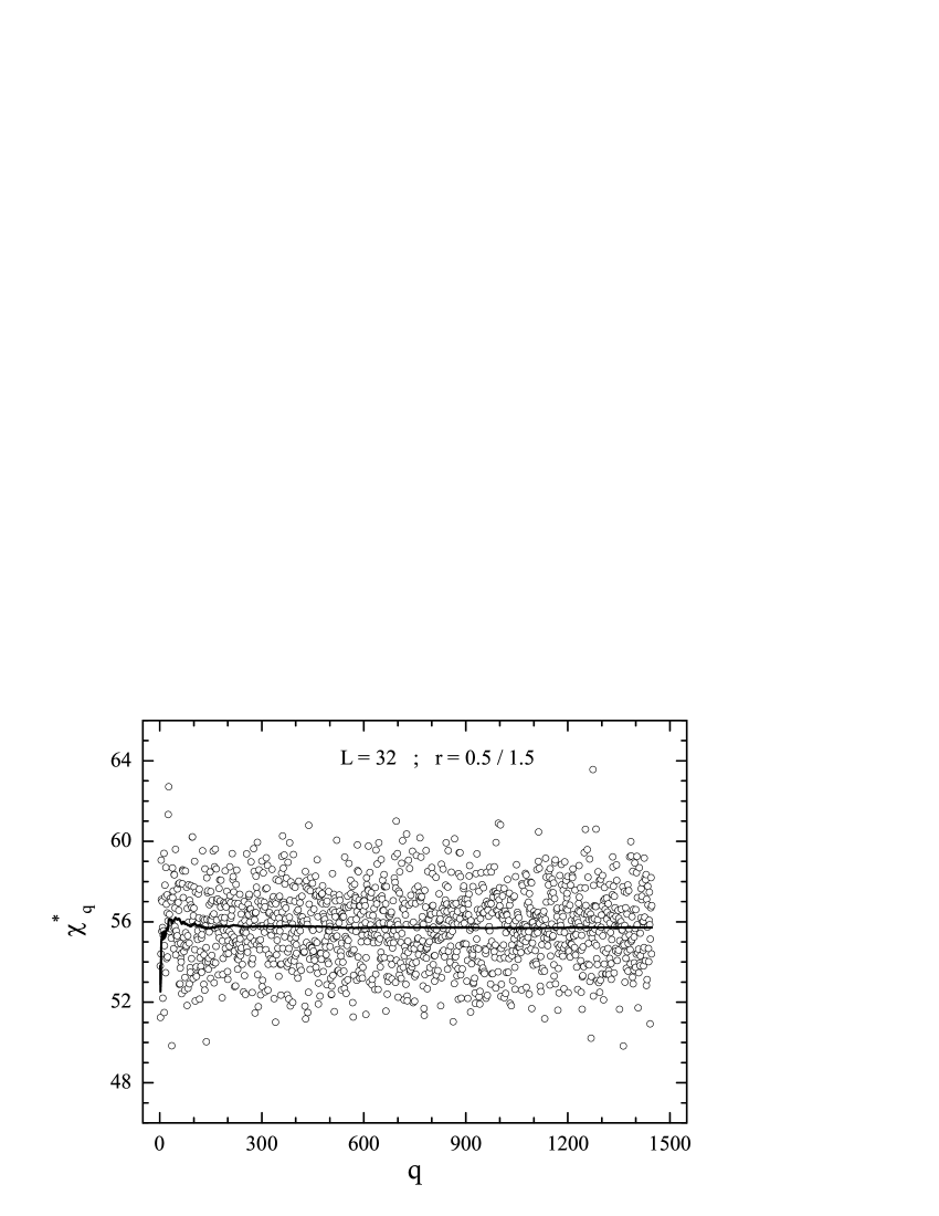
Figure 1: Disorder distribution of the susceptibility maxima of a lattice with linear size $L=32$ for disorder strength $r=0.5/1.5$. The running average over the samples is shown by the thick solid line.

The process continues in two further stages (two-stage process), using now mainly high iteration levels, where the modification factor is very close to unity and there is not any significant violation of the detailed balance condition during the WL process. These two stages are suitable for the accumulation of histogram data (for instance, energy-magnetization histograms), which can be used for an accurate entropic calculation of non-thermal thermodynamic parameters, such as the order parameter and its susceptibility malakis-04b . In the first (high-level) stage, we follow again a repeated several times (typically $\sim 5-10$) multi-R WL approach, carried out now only in the restricted energy subspace. The WL levels may be now chosen as $j=18,19,20$ and as an appropriate starting DOS for the corresponding starting level the average DOS of the preliminary stage at the starting level may be used. Finally, the second (high-level) stage is applied in the refinement WL levels $j=j_{i},\ldots,j_{i}+3$ (typically $j_{i}=21$), where we usually test both an one-range (one-R) or a multi-R approach with large energy intervals. In the case of the one-R approach we have found very convenient and more accurate to follow the Belardinelli-Pereyra belardinelli-07 adjustment of the WL modification factor according to the rule $\ln f\sim t^{-1}$. Finally, it should be also noted that by applying in our scheme a separate accumulation of histogram data in the starting multi-R stage (in the wide energy subspace) offers the opportunity to inspect the behavior of all basic thermodynamic functions in an also wide temperature range and not only in the neighborhood of the finite-size anomalies.

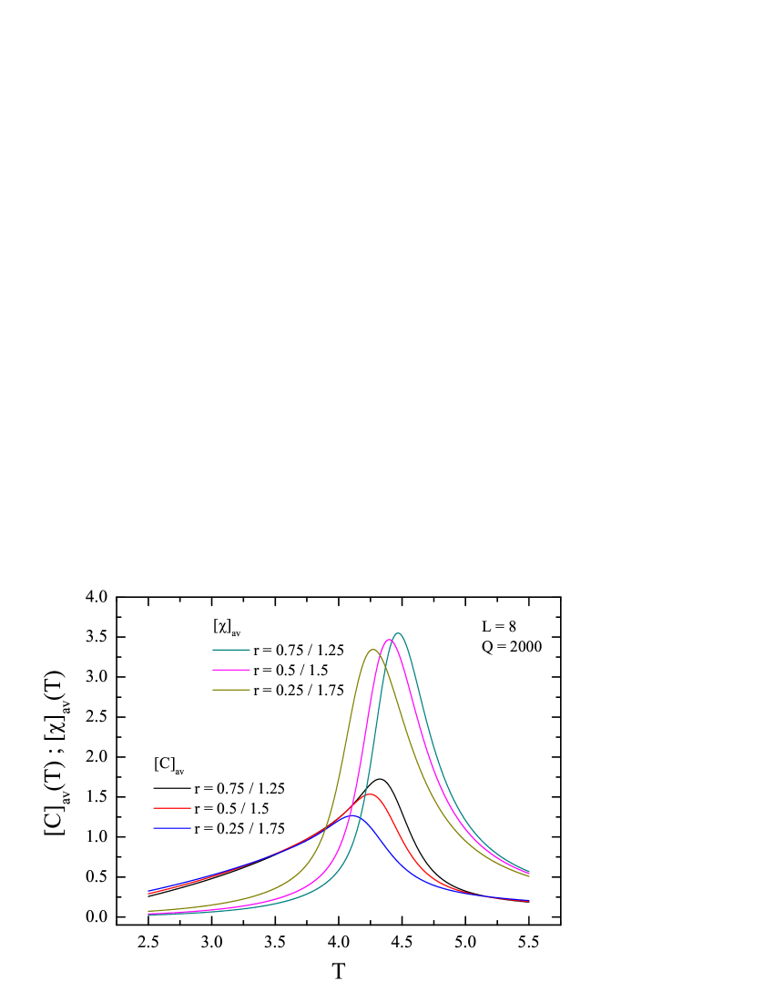
Figure 2: (Color online) Disorder-averaged specific heat $[C]_{av}$ (lower curves) and magnetic susceptibility $[\chi]_{av}$ (upper curves) as a function of the temperature $T$ for a lattice with linear size $L=8$. The ensemble of random realizations is $Q=2000$ for all cases of the disorder strength shown here. Notice the expected shift of the pseudocritical temperatures to the left with increasing the disorder strength ($r\rightarrow 0$).

Using this scheme we performed extensive simulations for several lattice sizes in the range $L=8-64$, over large ensembles $\{1,\cdots,q,\cdots,Q\}$ of random realizations ($Q=1000-3000$). It is well known that, extensive disorder averaging is necessary for the study of random systems, where usually broad distributions are expected leading to a strong violation of self-averaging wiseman-98 ; aharony-96 . A measure from the scaling theory of disordered systems, whose limiting behavior is directly related to the issue of self-averaging wiseman-98 ; aharony-96 may be defined with the help of the relative variance of the sample-to-sample fluctuations of any relevant singular extensive thermodynamic property $Z$ as follows: $R_{Z}=([Z^{2}]_{av}-[Z]^{2}_{av})/[Z]^{2}_{av}$. Figure 1 presents evidence that the above number of random realizations is sufficient in order to obtain the true average behavior and not a typical one. In particular, we plot in this figure (for a lattice size $L=32$ and disorder strength $r=0.5/1.5$) the disorder distribution of the susceptibility maxima $\chi_{q}^{\ast}$ (where the subscript $q$ denotes the random realization) and the corresponding running average, i.e., a series of averages of different subsets of the full data set - each of which is the average of the corresponding subset of a larger set of data points, over the samples for the simulated ensemble of $Q=1447$ disorder realizations. A first striking observation from this figure is the existence of very large variance of the values of $\chi_{q}^{\ast}$, indicating the violation of self-averaging for this quantity wiseman-98 ; aharony-96 . This figure illustrates that the simulated number of random realizations is sufficient in order to probe correctly the average behavior of the system, since already for $Q\approx 300$ the average value of $\chi^{\ast}_{q}$ is stable.

Closely related to the above issue of self-averaging in disordered systems is the manner of averaging over the disorder bernardet-00 . This non-trivial process may be performed in two distinct ways when identifying the finite-size anomalies, such as the peaks of the magnetic susceptibility. The first way corresponds to the average over disorder realizations ($[\ldots]_{av}$) and then taking the maxima ($[\ldots]^{\ast}_{av}$), or taking the maxima in each individual realization first, and then taking the average ($[\ldots^{\ast}]_{av}$). In the present paper we present our FSS analysis using mainly the first approach of averaging, although we should note that also the second gave comparable results. As an example, we show in Figure 2 the curves of the specific heat and magnetic susceptibility for a lattice with linear size $L=8$ averaged over $Q=2000$ random realizations. One may retrieve the location of the pseudocritical point by taking the maximum of these curves. Commenting on the statistical errors of our WL scheme, we found that the statistical errors of our scheme on the observed average behavior were of small magnitude (of the order of the symbol sizes) and thus are neglected in the figures. On the other hand, for the case $[\ldots^{\ast}]_{av}$ the error bars shown reflect the sample-to-sample fluctuations.

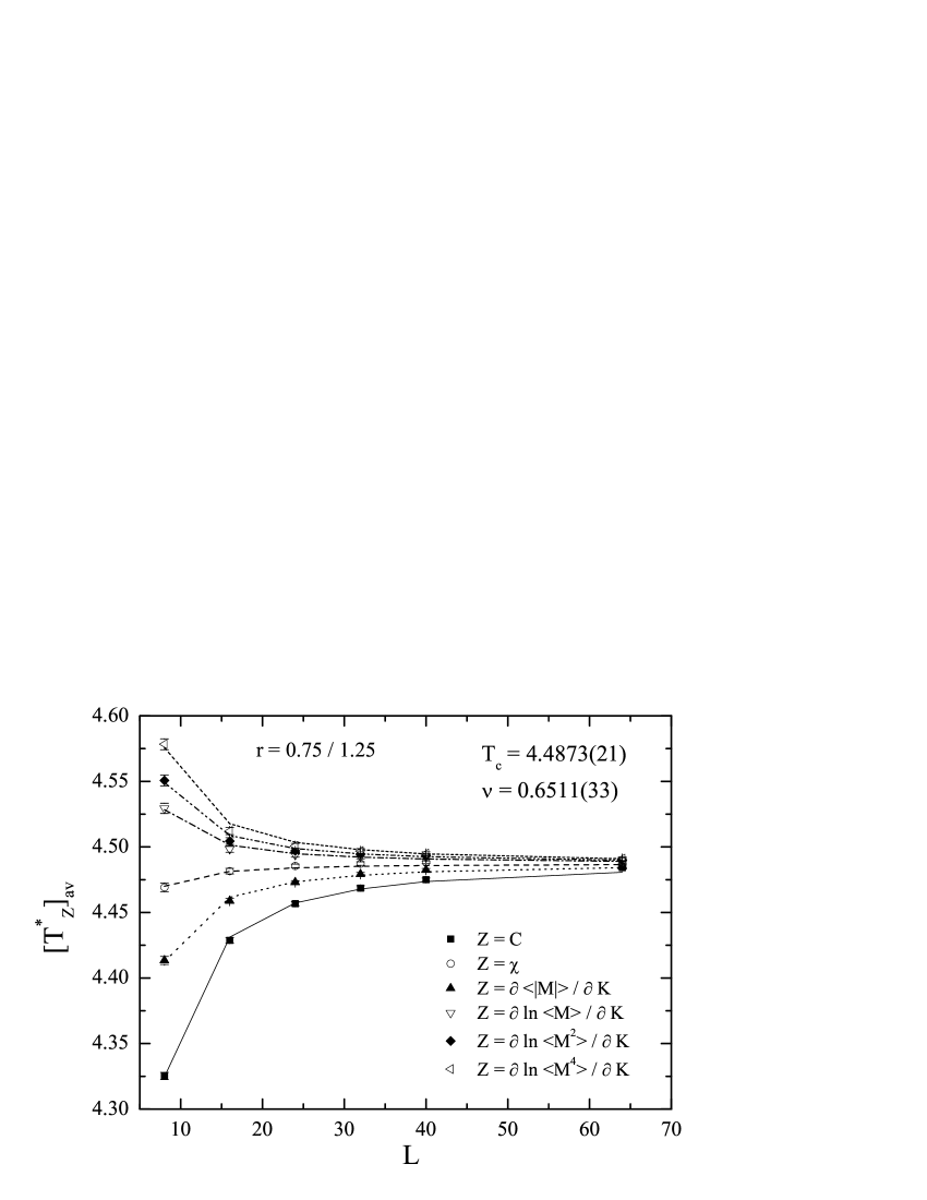
Figure 3: Shift behavior of several pseudocritical temperatures defined in the text for $r=0.75/1.25$. The error bars reflect the sample-to-sample fluctuations.

3 Numerical results and discussion

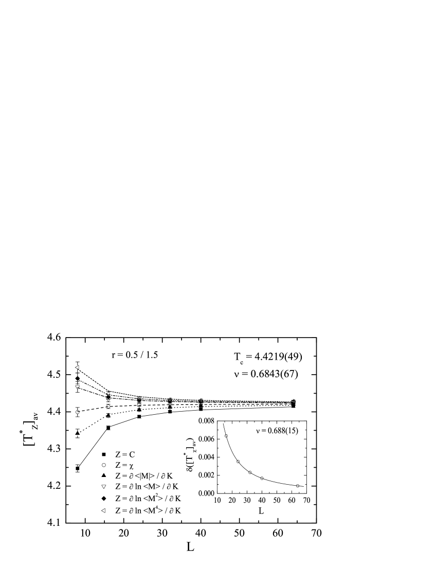
Figure 4: Same as Figure 3, but for $r=0.5/1.5$. The inset shows the FSS of the sample-to-sample fluctuations of the pseudocritical temperature of the magnetic susceptibility.

We present in this Section our numerical results and FSS analysis for the 3D random-bond Ising model. In Figures 3 - 5 we illustrate in the main panels the shift behavior of several pseudocritical temperatures, i.e., we take the average over the pseudocritical temperatures of the individual samples. In all cases the error bars reflect the sample-to-sample fluctuations. The considered pseudocritical temperatures correspond to the peaks of the following six quantities: specific heat $C$, magnetic susceptibility $\chi$, derivative of the absolute order parameter with respect to inverse temperature $K=1/T$ ferrenberg-91

$$\partial\langle|M|\rangle/\partial K=\langle|M|H\rangle-\langle|M|\rangle\langle H\rangle$$ (3)

and logarithmic derivatives of the first ($n=1$), second ($n=2$), and fourth ($n=4$) powers of the order parameter with respect to inverse temperature ferrenberg-91

$$\partial\ln\langle M^{n}\rangle/\partial K=\langle M^{n}H\rangle/\langle M^{n}\rangle-\langle H\rangle.$$ (4)

Fitting our data for the whole lattice range to the expected power-law behavior

$$[T^{\ast}_{Z}]_{av}=T_{c}+bL^{-1/\nu},$$ (5)

where $Z$ stands for the different thermodynamic quantities mentioned above, we estimate the critical temperatures as a function of the disorder strength and the respective critical exponents of the correlation length. In particular, for the case of very weak disorder (case $r=0.75/1.25$ shown in Figure 3) we estimate a value $T_{c}=4.4873(21)$ for the critical temperature and $\nu=0.6511(33)$ for the respective critical exponent. Although this value of $\nu$ is larger than the corresponding value of the pure system, it is still far away from the expected value of the random system (as obtained in references ball-98 ; berche-04 ; fytas-10 and Figures 4 and 5). This is due to finite-size effects that dominate in the regime of very weak randomness, hindering the approach of the system to the asymptotic limit. On the other hand, the simultaneous fittings of the form (5) shown in the main panels of Figures 4 and 5 for stronger values of the disorder strength $r$ reveal estimates for the correlation length exponent $\nu$ around the value $0.6849(50)$, in excellent agreement with the values $0.6837(53)$ and $0.68(2)$ given by Ballesteros et al. ball-98 and Berche et al. berche-04 for the site- and bond-diluted models. Additionally, the estimated values for the critical temperatures, in all Figures 3, 4, and 5, follow the usual reduction trend with increasing disorder strength ($r\rightarrow 0$), as already shown in Figure 2 of Section 2.

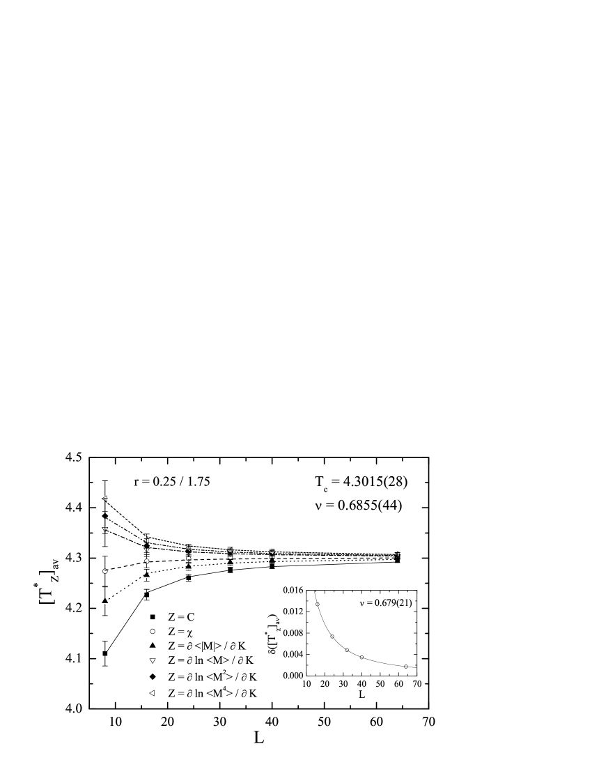
Figure 5: Same as Figure 4 but for the case $r=0.25/1.75$.

Using the above sample-to-sample fluctuations of the pseudocritical temperatures and the theory of FSS in disordered systems as introduced by Aharony and Harris aharony-96 and Wiseman and Domany wiseman-98 , one may further examine the nature of the fixed point controlling the critical behavior of the disordered system. According to the theoretical predictions aharony-96 ; wiseman-98 , the pseudocritical temperatures $T_{Z}^{\ast}$ of the disordered system are distributed with a width $\delta[T_{Z}^{\ast}]_{av}$, that scales, in the case of a new random fixed point, with the system size as

$$\delta([T_{Z}^{\ast}]_{av})\sim L^{-1/\nu}.$$ (6)

In the insets of Figures 4 and 5 we plot these sample-to-sample fluctuations of the pseudocritical temperature of the magnetic susceptibility. The solid lines show, in both cases, a very good power-law fitting giving the values $0.688(15)$ and $0.679(21)$ for the exponent $\nu$, which is also in very good agreement with the values denoted above and obtained via the classical shift behavior and the accurate estimates in the literature ball-98 ; berche-04 .

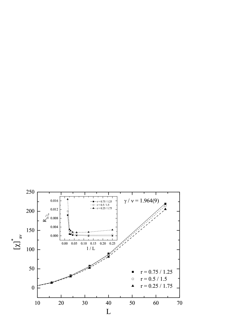
Figure 6: FSS of the maxima of the disorder-averaged magnetic susceptibility for all the three values of the disorder strength considered. The solid, dotted, and dashed lines show a simultaneous fitting attempt of the form $[\chi]_{av}^{\ast}\sim L^{\gamma/\nu}$ for the range $L=16-64$. The inset shows the corresponding limiting behavior of the ratio $R_{[\chi^{\ast}]_{av}}$ as defined in the text.

We move now to investigate the magnetic properties of the model. In Figure 6 we provide estimates for the magnetic exponent ratio $\gamma/\nu$ of the 3D random-bond Ising model, by presenting the FSS behavior of the maxima of the disorder-averaged magnetic susceptibility $[\chi]_{av}^{\ast}$ for all the values of the disorder strength considered. The solid, dotted, and dashed lines show a simultaneous fitting of the form

$$[\chi]_{av}^{\ast}\sim L^{\gamma/\nu},$$ (7)

using the $L=16-64$ lattice-range spectrum, providing an estimate $1.964(9)$ for the exponent ratio $\gamma/\nu$. We remind the reader that the respective fitting attempts of the numerical data for each case separately gave the estimates $\gamma/\nu=1.962(4)$, $1.967(3)$, and $1.969(4)$, for $r=0.75/1.25$, $0.5/1.5$, and $0.25/1.75$, respectively. All these sets of values are in excellent agreement with the accurate estimates $1.963(5)$ of reference ball-98 and $1.97(2)$ of reference berche-04 for the ratio $\gamma/\nu$ of the site- and bond-diluted models, respectively. In the corresponding inset of Figure 6 we try to further quantify the behavior of the sample-to-sample fluctuations of the model by plotting the noise to signal ratio $R_{Z}$ - already introduced in Section 2 - as a function of the inverse lattice size, for $Z=[\chi^{\ast}]_{av}$. Clearly, for the present model the limiting value of $R_{[\chi^{\ast}]_{av}}$ is nonzero, indicating, as expected also for marginal disordered systems wiseman-98 , a strong violation of self-averaging of the magnetic properties of the 3D Ising model with bond disorder, a property that intensifies with increasing disorder strength ($r\rightarrow 0$). We should comment here that analogous behavior of the ratio $R_{[\chi^{\ast}]_{av}}$ has been observed also in several other 3D and 2D random models, some of them being the bond- berche-04 and site-diluted ball-98 versions of the present 3D Ising model and the random-bond versions of the square Blume-Capel malakis-09 and triangular Ising fytas-10b model. As a final remark, we stress that the asymptotic behavior of these $R$-ratios is expected, from theoretical renormalization-group arguments, to follow specific power law functions and reach limiting values independent of the value of the disorder strength aharony-96 . However, such an analysis is by far much more demanding, in terms of numerical data, as it has already been discussed by Berche et al. berche-04 , and, in any case, goes beyond the scope of the present work.

Respectively, in Figure 7 we plot the disorder-averaged magnetization at the estimated critical temperatures of the disordered model, as a function of the lattice size $L$. The solid, dotted, and dashed lines show a simultaneous fitting following the well-known relation

$$[M]_{av}(T=T_{c})\sim L^{-\beta/\nu},$$ (8)

giving an estimate of the order of $0.517(5)$ for the exponent ratio $\beta/\nu$. Let us note here that, as in the case of the magnetic susceptibility in Figure 6, the respective separate fitting attempts of the numerical data gave comparable to the $0.517$ estimates in the regime $0.511-0.522$. Additional estimates for this exponent ratio can be obtained from the FSS of the derivative of the absolute order parameter with respect to inverse temperature $\partial\langle|M|\rangle/\partial K$. Thus, in the corresponding inset of Figure 7 we plot the data for $\partial\langle|M|\rangle/\partial K$ averaged over disorder as a function of $L$, in a double logarithmic scale. Their maxima are expected to scale with the system size as ferrenberg-91

$$(\partial\langle|M|\rangle/\partial K)^{\ast}\sim L^{(1-\beta)/\nu}.$$ (9)

As in the main panel, the three lines shown in the inset correspond to linear fittings for the three values of the disorder strength, verifying the estimates of the main panel of the figure for $\beta/\nu$, being also in very good agreement with accurate estimates $0.519(3)$ ball-98 and $0.515(5)$ berche-04 for the site- and bond-diluted models, respectively.

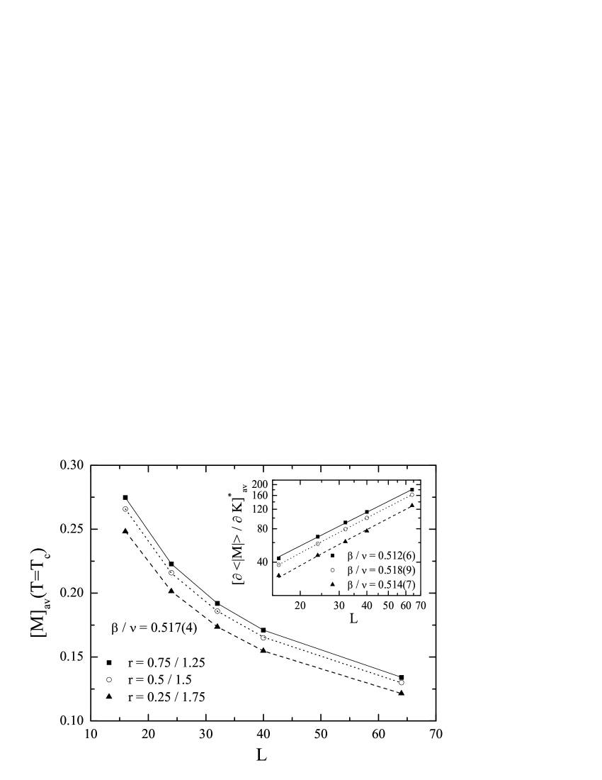
Figure 7: FSS of the disorder-averaged order parameter at the estimated critical temperatures $T_{c}(r)$ for $r=0.75/1.25$, $0.5/1.5$, and $0.25/1.75$. The inset illustrates the FSS of the maxima of the disorder-averaged inverse-temperature derivative of the absolute order parameter. In both main panel and inset, lattices with linear sizes $L=16-64$ have been used in the fittings.

Overall, the estimates for the critical exponent $\nu$ of the correlation length and the magnetic exponent ratios $\gamma/\nu$ and $\beta/\nu$ given in this Section, and summarized in Table 1, are in excellent agreement with accurate estimates in the literature for the respective site- ball-98 and bond-diluted models berche-04 , reinforcing the scenario of a single distinctive universality class in the 3D Ising model with quenched uncorrelated disorder, indicating the presence of a new random fixed point.

4 Summary and outlook

In summary, we reported in the present paper the effects induced by the presence of quenched bond randomness on the critical behavior of the 3D Ising spin model embedded in the simple cubic lattice, by implementing an efficient two-stage entropic simulation scheme based on the Wang-Landau algorithm. Our numerical approach enabled us to simulate large ensembles of disorder realizations of the model for very large lattice sizes (up to $N=64^{3}$) and several disorder strengths, and thus, obtain, via finite-size scaling techniques, accurate estimates of all the critical exponents describing the phase transition of the model. Particular interest was paid to the sample-to-sample fluctuations of the pseudocritical temperatures of the model and their scaling behavior that was used as a successful alternative approach to criticality.

The main conclusion of this study can be synopsized as follows: the critical behavior of the 3D Ising model with quenched uncorrelated disorder is controlled by a new random fixed point, independently of the way randomness is implemented in the system. It should be acknowledged at this point that, Ballesteros et al. ball-98 and Berche et al. berche-04 were the first scientific groups that strongly supported the above view for the present model. However, we believe that the results brought forward in this paper, combined with the existing ones for the site- and bond-diluted models, complete the picture, at least for this specific case of the 3D disordered Ising model, contributing further to the understanding of the concept of universality in disordered spin models.

Table 1: Summary of critical exponents for the pure and disordered 3D Ising model. The values of references guida-98 , ball-98 , and berche-04 have been used for the pure, site-, and bond-diluted versions of the model.

Disorder Distribution	$\nu$	$\gamma/\nu$	$\beta/\nu$
None (Pure model)	0.6304(13)	1.966(3)	0.517(3)
Site dilution	0.6837(53)	1.963(5)	0.519(3)
Bond dilution	0.68(2)	1.97(2)	0.515(5)
Bond randomness	0.685(7)	1.964(9)	0.517(4)

Closing, we stress here that it would be interesting to study further the universality aspects of even more complicated spin models, in terms of different disorder distributions and couplings. One interesting case would be to consider field-disorder coupling to the local order parameter, and one prominent candidate for this case is the 3D random-field Ising model vink-10 ; sourlas-99 . Of course for this type of model one may be particularly careful, since in this case there exist the well-known hyperscaling violation and new scaling concepts should be taken under serious account vink-10 ; sourlas-99 ; fytas-11 . Several attempts towards this direction of understanding universality in random systems are currently under consideration on both numerical and theoretical grounds.

References

- (1) Spin glasses and random fields, edited by A.P. Young (World Scientific, Singapore, 1998)
- (2) M. Aizenman, J. Wehr, Phys. Rev. Lett. 62, 2503 (1989)
- (3) M. Aizenman, J. Wehr, Phys. Rev. Lett. 64, 1311(E) (1990)
- (4) K. Hui, A.N. Berker, Phys. Rev. Lett. 62, 2507 (1989)
- (5) K. Hui, A.N. Berker, Phys. Rev. Lett. 63, 2433(E) (1989)
- (6) S. Chen, A.M. Ferrenberg, D.P. Landau, Phys. Rev. Lett. 69, 1213 (1992)
- (7) J. Cardy, J.L. Jacobsen, Phys. Rev. Lett. 79, 4063 (1997)
- (8) C. Chatelain, B. Berche, Phys. Rev. Lett. 80, 1670 (1998)
- (9) A.B. Harris, J. Phys. C 7, 1671 (1974)
- (10) J.T. Chayes, L. Chayes, D.S. Fisher, T. Spencer, Phys. Rev. Lett. 57, 2999 (1986)
- (11) V. Dotsenko, M. Picco, P. Pujol, Nucl. Phys. B 455, 701 (1995)
- (12) J.L. Jacobsen, J. Cardy, Nucl. Phys. B 515, 701 (1998)
- (13) G. Mazzeo, R. Kühn, Phys. Rev. E 60, 3823 (1999)
- (14) A. Gordillo-Guerrero, R. Kenna, J.J. Ruiz Lorenzo, AIP Conf. Proc. 1198, 42 (2009)
- (15) D.P. Landau, Phys. Rev. B 22, 2450 (1980)
- (16) D. Chowdhury, D. Stauffer, J. Stat. Phys. 44, 203 (1986)
- (17) H.-O. Heuer, Europhys. Lett. 12, 551 (1990)
- (18) H.-O. Heuer, Phys. Rev. B 42, 6476 (1990)
- (19) H.-O. Heuer, J. Phys. A 26, L333 (1993)
- (20) M. Hennecke, Phys. Rev. B 48, 6271 (1993)
- (21) H.G. Ballesteros, L. A. Fernández, V. Martín-Mayor, A. Muñoz Sudupe, G. Parisi, J. J. Ruiz-Lorenzo, Phys. Rev. B 58, 2740 (1998)
- (22) S. Wiseman, E. Domany, Phys. Rev. Lett. 81, 22 (1998)
- (23) P. Calabrese, V. Martín-Mayor, A. Pelissetto, E. Vicari, Phys. Rev. E 68, 036136 (2003)
- (24) M. Hasenbusch, F. Parisen Toldin, A. Pelissetto, E. Vicari, J. Stat. Mech.: Theory Exp. 2007, P02016
- (25) P.E. Berche, C. Chatelain, B. Berche, W. Janke, Eur. Phys. J. B 38, 463 (2004)
- (26) R. Folk, Y. Holovatch, T. Yavors kii, Phys. Rev. B 61, 15114 (2000)
- (27) D.V. Pakhnin, A.I. Sokolov, Phys. Rev. B 61, 15130 (2000)
- (28) A. Pelissetto, E. Vicari, Phys. Rev. B 62, 6393 (2000)
- (29) K.E. Newman, E.K. Riedel, Phys. Rev. B 25, 264 (1982)
- (30) G. Jug, Phys. Rev. B 27, 609 (1983)
- (31) I.O. Mayer, J. Phys. A 22, 2815 (1989)
- (32) R. Guida, J. Zinn-Justin, J. Phys. A 31, 8103 (1998)
- (33) A.K. Murtazaev, A.B. Babaev, J. Magn. Magn. Mater. 321, 2630 (2009)
- (34) N.G. Fytas, P.E. Theodorakis, Phys. Rev. E 82, 062101 (2010)
- (35) M.E.J. Newman, G.T.Barkema, Monte Carlo Methods in Statistical Physics (Clarendon Press, Oxford, 1999)
- (36) F. Wang, D.P. Landau, Phys. Rev. Lett. 86, 2050 (2001)
- (37) F. Wang, D.P. Landau, Phys. Rev. E 64, 056101 (2001)
- (38) A. Malakis, A. Peratzakis, N.G. Fytas, Phys. Rev. E 70, 066128 (2004)
- (39) A. Malakis, S.S. Martinos, I.A. Hadjiagapiou, N.G. Fytas, P. Kalozoumis, Phys. Rev. E 72, 066120 (2005)
- (40) A. Malakis, N.G. Fytas, Phys. Rev. E 73, 016109 (2006)
- (41) N.G. Fytas, A. Malakis, K. Eftaxias, J. Stat. Mech.: Theory Exp. (2008) P03015
- (42) N.G. Fytas, A. Malakis, I.A. Hadjiagapiou, J. Stat. Mech.: Theory Exp. (2008) P11009
- (43) A. Malakis, A.N. Berker, I.A. Hadjiagapiou, N.G. Fytas, T. Papakonstantinou, Phys. Rev. E 81, 041113 (2010)
- (44) N.G. Fytas, A. Malakis, Phys. Rev. E 81, 041109 (2010)
- (45) R.E. Belardinelli, V.D. Pereyra, Phys. Rev. E 75, 046701 (2007)
- (46) A. Aharony, A.B. Harris, Phys. Rev. Lett. 77, 3700 (1996)
- (47) K. Bernardet, F. Pázmándi, G.G. Batrouni, Phys. Rev. Lett. 84, 4477 (2000)
- (48) A.M. Ferrenberg, D.P. Landau, Phys. Rev. B 44, 5081 (1991)
- (49) R.L.C. Vink, T. Fischer, K. Binder, Phys. Rev. E 82, 051134 (2010)
- (50) N. Sourlas, Comput. Phys. Commun. 121, 183 (1999)
- (51) N.G. Fytas, A. Malakis, Eur. Phys. J. B 79, 13 (2011)