An Optimal Real-Time Scheduling Approach:
From Multiprocessor to Uniprocessor

Abstract

An optimal solution to the problem of scheduling real-time tasks on a set of identical processors is derived. The described approach is based on solving an equivalent uniprocessor real-time scheduling problem. Although there are other scheduling algorithms that achieve optimality, they usually impose prohibitive preemption costs. Unlike these algorithms, it is observed through simulation that the proposed approach produces no more than three preemptions points per job.

I Introduction

I-A Motivation

Scheduling $n$ real-time tasks on $m$ processors is a problem that has taken considerable attention in the last decade. The goal is to find a feasible schedule for these tasks, that is a schedule according to which no task misses its deadlines. Several versions of this problem have been addressed and a number of different solutions have been given. One of the simplest versions assumes a periodic-preemptive-independent task model with implicit deadlines, PPID for short. According to the PPID model each task is independent of the others, jobs of the same task are released periodically, each job of a task must finish before the release time of its successor job, and the system is fully preemptive.

A scheduling algorithm is considered optimal if it is able to find a feasible schedule whenever one exists. Some optimal scheduling algorithms for the PPID model have been found. For example, it has been shown that if all tasks share the same deadline [1], the system can be optimally scheduled with a very low implementation cost. The assumed restriction on task deadlines, however, prevents the applicability of this approach. Other optimal algorithms remove this restriction but impose a high implementation cost due to the required number of task preemptions [2, 3, 4]. It is also possible to find trade-offs between optimality and preemption cost [5, 6, 7, 8].

Optimal solutions for the scheduling problem in the PPID model are able to create preemption points that make it possible task migrations between processors allowing for the full utilization of the system. As illustration consider that there are three tasks, $\tau_{1}$, $\tau_{2}$ and $\tau_{3}$, to be scheduled on two processors. Suppose that each of these tasks requires $2$ time units of processor and must finish $3$ time units after they are released. Also, assume that all three tasks have the same release time. As can be seen in Figure 1, if two of these tasks are chosen to execute at their release time and they are not preempted, the pending task will miss its deadline. As all tasks share the same deadline in this example, the approach by McNaughton [1] can be applied, as illustrated in the figure. If this was not the case, generating possibly infinitely many preemption points could be a solution as it is shown by other approaches [2, 3, 4]. In this work we are interested in a more flexible solution.

(a) C misses its deadline

(b) Correct schedule

Figure 1: A deadline miss occurs in case (a), but not in case (b).

I-B Contribution

In the present work, we define a real-time task as an infinite sequence of jobs. Each job represents a piece of work to be executed on one or more processors. A job is characterized by its release time $r$, time after which it can be executed, and its deadline $d$, time by which it must be completed in order for the system to be correct. Also, we assume that the deadline of a job is equal to the release time of the next job of the same task. However, differently from the PPID model, we do not assume that tasks are necessarily periodic. Instead, we assume that tasks have a fixed-utilization, i. e. each job of a task utilizes a fixed processor bandwidth within the interval between its release time and deadline. For example, a job of a task with utilization $u\leqslant 1$ of processor requires $u(d-r)$ execution time. Note that according to the PPID model, the value $d-r$ is equal to the period of the periodic task, which makes the model assumed in this paper slightly more general than the PPID model.

The proposed approach is able to optimally schedule a set of fixed-utilization tasks on a multiprocessor system. The solution we describe does not impose further restrictions on the task model and only a few preemption points per job are generated. The idea is to reduce the real-time multiprocessor scheduling problem into an equivalent real-time uniprocessor scheduling problem. After solving the latter, the found solution is transformed back to a solution to the original problem. This approach seems very attractive since it makes use of well known results for scheduling uniprocessor systems.

Consider the illustrative system with 3-tasks previously given. We show that scheduling this system on two processors is equivalent to scheduling another 3-task system with tasks $\tau_{1}^{*}$, $\tau_{2}^{*}$ and $\tau_{3}^{*}$ on one processor. Each star task requires one unit of time and has the same deadline as the original task, that is the star tasks represent the slack of the original ones. As can be seen in Figure 2, the basic scheduling rule is the following. Whenever the star task executes on the transformed system, its associated original task does not execute on the original system. For example, when $\tau_{1}^{*}$ is executing on the transformed system, task $\tau_{1}$ is not executing on the original system.

Figure 2: Scheduling equivalence of $\tau_{1}^{*}$, $\tau_{2}^{*}$ $\tau_{3}^{*}$ on one processor and $\tau_{1}$, $\tau_{2}$, $\tau_{3}$ on two processors.

The illustrative example gives only a glimpse of the proposed approach and does not capture the powerfulness of the solution described in this document. For example, if the illustrative example had four tasks instead of three, the scheduling rule could not be applied straightforwardly. For such cases, we show how to aggregate tasks so that the reduction to the uniprocessor scheduling problem is still possible. For more general cases, a series of system transformation, each one generating a system with fewer processors, may be applied. Once a system with only one processor is obtained, the well known EDF algorithm is used to generate the correct schedule. Then, it is shown that this schedule can be used to correctly generate the schedule for the original multiprocessor system.

I-C Structure

In the remainder of this paper we detail the proposed approach. The notation and the assumed model of computation are described in Section II. Section III presents the concept of servers, which are a means to aggregate tasks (or servers) into a single entity to be scheduled. In Section IV it is shown the rules to transform a multiprocessor system into an equivalent one with fewer processors and the scheduling rules used. The correctness of the approach is also shown in this section. Then, experimental results collected by simulations are presented in Section V. Finally, Section VI gives a brief summary on related work and conclusions are drawn in Section VII.

II System Model and Notation

II-A Fixed-Utilization Tasks

As mentioned earlier, we consider a system comprised of $n$ real-time and independent tasks, each of which defines an infinite sequence of released jobs. More generally, a job can be defined as follows.

Definition II.1 (Job).

A real-time job, or simply, job, is a finite sequence of instructions to be executed. If $J$ is a job, it admits a release time, denoted $J.r$, an execution requirement, denoted $J.c$, and a deadline, denoted $J.d$.

In order to represent possibly non-periodic execution requirements, we introduce a general real-time object, called fixed-utilization task, or task for short, whose execution requirement is specified in terms of processor utilization within a given interval. Since a task shall be able to execute on a single processor, its utilization cannot be greater than one.

Definition II.2 (Fixed-Utilization Task).

Let $u$ be a positive real not greater than one and let $D$ be a countable and unbounded set of non-negative reals. The fixed-utilization task $\tau$ with utilization $u$ and deadline set $D$, denoted $\tau\mspace{-5.0mu}:\mspace{-5.0mu}(u,D)$, satisfies the following properties: (i) a job of $\tau$ is released at time $t$ if and only if $t\in D$; (ii) if $J$ is released at time $r$, then $J.d=\min_{t}\{t\in D,t>J.r\}$; and (iii) $J.c=u(J.d-J.r)$.

Given a fixed-utilization task $\tau$, we denote $\mu(\tau)$ and $\Lambda(\tau)$ its utilization and its deadline set, respectively.

As a simple example of fixed-utilization task, consider a periodic task $\tau$ characterized by three attributes: (i) its start time $\,s$; (ii) its period $T$; and (iii) its execution requirement $C$. Task $\tau$ generates an infinite collection of jobs each of which released at $s+(j-1)T$ and with deadline at $s+jT$, $j\in\mathbb{N}^{*}$. Hence, $\tau$ can be seen as a fixed-utilization task with start time at $s$, utilization $\mu(\tau)=C/T$ and set of deadlines $\Lambda(\tau)=\{(s+jT),j\in\mathbb{N}^{*}\}$, which requires exactly $\mu(\tau)T$ of processor during periodic time intervals $[s+(j-1)T,s+jT)$, for $j$ in $\in\mathbb{N}^{*}$. As will be clearer later on, the concept of fixed-utilization task will be useful to represent non-periodic processing requirements, such as those required by groups of real-time periodic tasks.

II-B Fully Utilized System

We say that a set of $n$ fixed-utilization tasks fully utilizes a system comprised of $m$ identical processors if the sum of the utilizations of the $n$ tasks exactly equals $m$. Hereafter, we assume that the set of $n$ fixed-utilization tasks fully utilizes the system.

It is important to mention that this assumption does not restrict the applicability of the proposed approach. For example, if a job $J$ of a task is supposed to require $J.c$ time units of processor but it completes consuming only $c^{\prime}<J.c$ processor units, then the system can easily simulate $J.c-c^{\prime}$ of its execution by blocking a processor accordingly. Also, if the maximum processor utilization required by the task set is less than $m$, dummy tasks can be created to comply with the full utilization assumption. Therefore, we consider hereafter that the full utilization assumption holds and so each job $J$ executes exactly for $u(J.d-J.r)$ time units during $[r,d)$.

II-C Global Scheduling

Jobs are assumed to be enqueued in a global queue and are scheduled to execute on a multiprocessor platform $\Pi$, comprised of $m>1$ identical processors. We consider a global scheduling policy according to which tasks are independent, preemptive and can migrate from a processor to another during their executions. There is no penalty associated with preemptions or migrations.

Definition II.3 (Schedule).

For any collection of jobs, denoted $\mathcal{J}$, and multiprocessor platform $\Pi$, the multiprocessor schedule $\Sigma$ is a mapping from $\,\mathbb{R}^{+}\times\mathcal{J}\times\Pi$ to $\{0,1\}$ with $\Sigma(t,J,\pi)$ equal to one if schedule $\Sigma$ assigns job $J$ to execute on processor $\pi$ at time $t$, and zero otherwise.

Note that by the above definition, the execution requirement of a job $J$ at time $t$ can be expressed as

$$e(J,t)=J.c-\sum_{\pi\in\Pi}\int_{J.r}^{t}\Sigma(t,J,\pi)dt,$$

Definition II.4 (Valid Schedule).

A schedule $\,\Sigma$ of a job set $\mathcal{J}$ is valid if (i) at any time, a single processor executes at most one job in $\mathcal{J}$; (ii) any job in $\mathcal{J}$ does not execute on more than one processor at any time; (iii) any job $J\in\mathcal{J}$ can only execute at time $t$ if $J.r\leqslant t$ and $e(J,t)>0$.

Definition II.5 (Feasible Schedule).

Let $\;\Sigma$ be a schedule of a set of jobs $\;\mathcal{J}$. The schedule $\Sigma$ is feasible if it is a valid schedule and if all the jobs in $\mathcal{J}$ finish executing by their deadlines.

We say that a job is feasible in a schedule $\Sigma$ if it finishes executing by its deadline, independently of the feasibility of $\Sigma$. That is, a job can be feasible in a non-feasible schedule. However, if $\Sigma$ is feasible, then all jobs scheduled in $\Sigma$ are necessarily feasible. Also, we say that a job $J$ is active at time $t$ if $J.r\leqslant t$ and $e(J,t)>0$. As a consequence, a fixed-utilization task admits a unique feasible and active job at any time.

III Servers

As mentioned before, the derivation of a schedule for a multiprocessor system will be done via generating a schedule for an equivalent uniprocessor system. One of the tools for accomplishing this goal is to aggregate tasks into servers, which can be seen as fixed-utilization tasks equipped with a scheduling mechanism.

As will be seen, the utilization of a server is not greater than one. Hence, in this section we will not deal with the multiprocessor scheduling problem. The focus here is on precisely defining the concept of servers (Section III-A) and showing how they correctly schedule the fixed-utilization tasks associated to them (Section III-B). In other words, the reader can assume in this section that there is a single processor in the system. Later on we will show how multiple servers are scheduled on a multiprocessor system.

III-A Server model and notations

A fixed-utilization server associated to a set of fixed-utilization tasks is defined as follows:

Definition III.1 (Fixed-Utilization Server).

Let $\mathcal{T}$ be a set of fixed-utilization tasks with total utilization given by

$$\mu(\mathcal{T})=\sum_{\tau\in\mathcal{T}}\mu(\tau)\leqslant 1$$

A fixed-utilization server $S$ associated to $\mathcal{T}$, denoted $\sigma(\mathcal{T})$, is a fixed-utilization task with utilization $\mu(\mathcal{T})$, set of deadlines $\Lambda(S)\subseteq\bigcup_{\tau\in\mathcal{T}}\Lambda(\tau)$, equipped with a scheduling policy used to schedule the jobs of the elements in $\mathcal{T}$. For any time interval $[d,d^{\prime})$, where $d,d^{\prime}\in\Lambda(S)$, $S$ is allowed to execute exactly for $\mu(\mathcal{T})(d^{\prime}-d)$ time units.

Given a fixed-utilization server $S$, we denote $\Gamma(S)$ the set of fixed-utilization tasks scheduled by $S$ and we assume that this set is statically defined before the system execution. Hence, the utilization of a server, simply denoted $\mu(S)$, can be consistently defined as equal to $\mu(\Gamma(S))$. Note that, since servers are fixed-utilization tasks, we are in condition to define the server of a set of servers. For the of sake of conciseness, we call an element of $\Gamma(S)$ a client task of $S$ and we call a job of a client task of $S$ a client job of $S$. If $S$ is a server and $\mathcal{T}$ a set of servers, then $\sigma(\Gamma(S))=S$ and $\Gamma(\sigma(\mathcal{T}))=\mathcal{T}$.

For illustration consider Figure 3, where $\mathcal{T}$ is a set comprised of the three servers $\sigma(\tau_{1})$, $\sigma(\tau_{2})$ and $\sigma(\tau_{3})$ associated to the fixed-utilization tasks $\tau_{1}$, $\tau_{2}$ and $\tau_{3}$, respectively. The numbers between brackets represent processor utilizations. If $S=\sigma(\mathcal{T})$ is the server in charge of scheduling $\sigma(\tau_{1})$, $\sigma(\tau_{2})$ and $\sigma(\tau_{3})$, then we have $\mathcal{T}=\Gamma(S)=\{\sigma(\tau_{1}),\sigma(\tau_{2}),\sigma(\tau_{3})\}$ and $\mu(S)=0.7$.

Figure 3: A three-server set. The utilization $u$ of a server $S$ or a set of server $\mathcal{T}$ is indicated by the notation $S^{(u)}$ and $\mathcal{T}^{(u)}$, respectively.

As can be seen by Definition III.1, the server $S$ associated to $\mathcal{T}$ may not have all the elements of $\bigcup_{\tau\in\mathcal{T}}\Lambda(\tau)$. Indeed, the number of elements in $\Lambda(S)$ depends on a server deadline assignment policy:

Definition III.2 (Server Deadline Assignment).

A deadline of a server $S$ at time $t$, denoted $\lambda_{S}(t)$, is given by the earliest deadline greater than $t$ among all client jobs of $S$ not yet completed at time $t$. This includes those jobs active at $t$ or the not yet released jobs at $t$. More formally,

$$\lambda_{S}(t)=\min_{J\in\mathcal{J}}\{J.d,(J.r<t\land e(J,t)>0)\;\lor\;J.r\geqslant t\}$$

where $\mathcal{J}$ is the set of all jobs of servers in $\Gamma(S)$.

Note that by Definitions II.2 and III.2, the execution requirement of a server $S$ in any interval $(d,d^{\prime})$ equals $\mu(S)(d^{\prime}-d)$, where $d$ and $d^{\prime}$ are two consecutive deadlines in $\Lambda(S)$. As a consequence, the execution requirement of a job $J$ of a server $S$, released at time $d\in\Lambda(S)$, equals $J.c=e(J,d)=\mu(S)(\lambda_{S}(d)-d)$ for all $d\in\Lambda(S)$. The budget of $S$ at any time $t$, denoted as $C_{S}(t)$, is replenished to $e(J,t)$ at all $t\in\Lambda(S)$. The budget of a server represents the processing time available for its clients. Although a server never executes itself, we say that a server $S$ is executing at time $t$ in the sense that one of its client tasks consumes its budget $C_{S}(t)$ at the same rate of its execution.

Recall from Section II-A that a job of an fixed-utilization task is feasible in a schedule $\Sigma$ if it meets its deadline. However, the feasibility of a server does not imply the feasibility of its client tasks. For example, consider two periodic tasks $\tau_{1}\mspace{-5.0mu}:\mspace{-5.0mu}(1/2,2\mathbb{N}^{*})$ and $\tau_{2}\mspace{-5.0mu}:\mspace{-5.0mu}(1/3,3\mathbb{N}^{*})$, with periods equal to 2 and 3 and utilizations $\mu(\tau_{1})=1/2$ and $\mu(\tau_{2})=1/3$, respectively. Assume that their start times are equal to zero. Consider a server $S$ scheduling these two tasks on a dedicated processor and let $\Lambda(S)=\{2,3,4,6,\ldots\}$. Thus, the budget of $S$ during $[0,2)$ equals $C_{S}(0)=2\mu(S)=5/3$. Let $\Sigma$ be a schedule of $\tau_{1}$ and $\tau_{2}$ in which $S$ is feasible. The feasibility of server $S$ implies that $S$ acquires the processor for at least $5/3$ units of time during $[0,2)$, since $2$ is a deadline of $S$. Now, suppose that the scheduling policy used by $S$ to schedule its client tasks gives higher priority to $\tau_{2}$ at time $0$. Then, $\tau_{2}$ will consume one unit of time before $\tau_{1}$ begins its execution. Therefore, the remaining budget $C_{S}(1)=2/3$ will be insufficient to complete $\tau_{1}$ by $2$, its deadline. This illustrates that a server can be feasible while the generated schedule of its clients is not feasible.

III-B EDF Server

In this section, we define an EDF server and shows that EDF servers are predictable in the following sense.

Definition III.3 (Predictable Server).

A fixed-utilization server $S$ is predictable in a schedule $\Sigma$ if its feasibility in $\Sigma$ implies the feasibility of all its client jobs.

Definition III.4 (EDF Server).

An EDF server is a fixed-utilization server $S$, defined according to Definitions III.1 and III.2, which schedules its client tasks by EDF.

For illustration, consider a set of three periodic tasks $\mathcal{T}=\{\mbox{$\tau_{1}\mspace{-5.0mu}:\mspace{-5.0mu}(1/3,3\mathbb{N}^{*})$},\mbox{$\tau_{2}\mspace{-5.0mu}:\mspace{-5.0mu}(1/4,4\mathbb{N}^{*})$},\mbox{$\tau_{3}\mspace{-5.0mu}:\mspace{-5.0mu}(1/6,6\mathbb{N}^{*})$}\}$. Since $\mu(\mathcal{T})=3/4\leqslant 1$, we can define an EDF server $S$ to schedule $\mathcal{T}$ such that $\Gamma(S)=\mathcal{T}$ and $\mu(S)=3/4$. Figure 4 shows both the evolution of $C_{S}(t)$ during interval $[0,12)$ and the schedule $\Sigma$ of $\mathcal{T}$ by $S$ on a single processor. In this figure, $i_{j}$ represents the $j$-th job of $\tau_{i}$. Observe here that $\Lambda(S)\neq\{3k,4k,6k|k\in\mathbb{N}^{*}\}$. Indeed, deadlines $4$ of $2_{1}$ and $9$ of $1_{3}$ are not in $\Lambda(S)$, since $2_{1}$ and $1_{3}$ are completed at time $3$ and $8$, respectively.

It is worth noticing that the deadline set of a server could be defined to include all deadlines of its clients. However, this would generate unnecessary preemption points.

Figure 4: Budget management and schedule of an EDF server $S$ with $\mathcal{T}(S)=\{\mbox{$\tau_{1}\mspace{-5.0mu}:\mspace{-5.0mu}(1/3,3\mathbb{N}^{*})$},\mbox{$\tau_{2}\mspace{-5.0mu}:\mspace{-5.0mu}(1/4,4\mathbb{N}^{*})$},\mbox{$\tau_{3}\mspace{-5.0mu}:\mspace{-5.0mu}(1/6,6\mathbb{N}^{*})$}\}$ and $\mu(S)=3/4$.

Definition III.5.

A set $\mathcal{T}$ of fixed-utilization tasks is a unit set if $\;\mu(\mathcal{T})=1$. The server $\sigma(\mathcal{T})$ associated to a unit set $\mathcal{T}$ is a unit server.

In order to prove that EDF servers are predictable, we first present some intermediate results.

Definition III.6.

Let $S$ be a server, $\mathcal{T}$ a set of servers with $\mu(\mathcal{T})\leqslant 1$, and $\alpha$ a real such that $0<\alpha\leqslant 1/\mu(S)$. The $\alpha$-scaled server of $S$ is the server with utilization $\alpha\mu(S)$ and deadlines equal to those of $S$. The $\alpha$-scaled set of $\mathcal{T}$ is the set of the $\alpha$-scaled servers of server in $\mathcal{T}$.

As illustration, consider $\mathcal{T}=\{S_{1},S_{2},S_{3}\}$ a set of servers with $\mu(\mathcal{T})=0.5$, $\mu(S_{1})=0.1$, $\mu(S_{2})=0.15$ and $\mu(S_{3})=0.25$. The $2$-scaled set of $\mathcal{T}$ is $\mathcal{T}^{\prime}=\{S_{1}^{\prime},S_{2}^{\prime},S_{3}^{\prime}\}$ with $\mu(\mathcal{T}^{\prime})=1$, $\mu(S_{1}^{\prime})=0.2$, $\mu(S_{2}^{\prime})=0.3$ and $\mu(S_{3}^{\prime})=0.5$.

Lemma III.1.

Let $\mathcal{T}$ be a set of EDF servers with $\mu(\mathcal{T})\leqslant 1$ and $\mathcal{T}^{\prime}$ be its $\alpha$-scaled set. Define $S$ and $S^{\prime}$ as two EDF servers associated to $\mathcal{T}$ and $\mathcal{T}^{\prime}$ and consider that $\,\Sigma$ and $\Sigma^{\prime}$ are their corresponding schedules, respectively. The schedule $\Sigma$ is feasible if and only if $\Sigma^{\prime}$ is feasible.

Proof:

Suppose $\Sigma$ feasible. Consider a deadline $d$ in $\Lambda(S)$. Since $S$ and $S^{\prime}$ use EDF and $\Lambda(S)=\Lambda(S^{\prime})$, $S$ and $S^{\prime}$ execute their client jobs in the same order. As a consequence, all the executions of servers in $\Gamma(S)$ during $[0,d)$ must have a corresponding execution of a server in $\Gamma(S^{\prime})$ during $[0,d)$.

Also, since $S$ executes for $\mu(S)d$ during $[0,d)$ and $\alpha\leqslant 1/\mu(S)$, the execution time $\mu(S^{\prime})d$ of $S^{\prime}$ during $[0,d)$ satisfies $\alpha\mu(S)d\leqslant d$. Hence, a client job of $S^{\prime}$ corresponding to an execution which completes in $\Sigma$ before $d$, completes before $d$ in $\Sigma^{\prime}$. Since $\Sigma$ is feasible, this shows that $\Sigma^{\prime}$ is feasible.

To show that $\Sigma$ is feasible if $\Sigma^{\prime}$ is feasible the same reasoning can be made with a scale equal to $\alpha^{\prime}=1/\alpha$ ∎

Lemma III.2.

The schedule of a set of servers $\mathcal{T}$ produced by the EDF server $S=\sigma(\mathcal{T})$ is feasible if and only if $\mu(\mathcal{T})\leqslant 1$.

Proof:

The proof presented here is an adaptation of the proof of Theorem $7$ from [9]. The difference between servers and tasks makes this presentation necessary.

First, assume that $\mu(\mathcal{T})>1$. Let $[d,d^{\prime})$ be a time interval with no processor idle time, where $d$ and $d^{\prime}$ are two deadlines of servers in $\mathcal{T}$. By the assumed utilization, this time interval must exist. As the cumulated execution requirement within this interval is $\mu(\mathcal{T})(d^{\prime}-d)>d^{\prime}-d$, a deadline miss must occur, which shows the necessary condition.

Suppose now that $d$ is the first deadline miss after time $t=0$ and let $S$ be the server whose job $J$ misses its deadline at $d$. Let $t^{\prime}$ be the start time of the latest idle time interval before $d$. Assume that $t^{\prime}=0$ if such a time does not exist. Also, let $d^{\prime}$ be the earliest deadline in $\Lambda(S)$ after $t^{\prime}$. Note that $d^{\prime}<d$ otherwise no job would be released between $t^{\prime}$ and $d$. If $d^{\prime}$ is not equal to zero, then the processor must be idle just before $d^{\prime}$. Indeed, if there were some job executing just before $d^{\prime}$, it would be released after $t^{\prime}$ and its release instant would be a deadline in $\Lambda(S)$ occurring before $d^{\prime}$ and after $t^{\prime}$, which would contradict the definition of $d^{\prime}$. Hence, only the time interval between $d^{\prime}$ and $d$ is to be considered. There are two cases to be distinguished depending on whether some lower priority server executes within $[d^{\prime},d)$.

Figure 5: A deadline miss occurs for job $J$ at time $d$ and no job with lower priority than $J$ executes before $d$

Case 1

Illustrated by Figure 5. Assume that no job of servers in $\Gamma(S)$ with lower priority than $J$ executes within $[d^{\prime},d)$. Since there is no processor idle time between $d^{\prime}$ and $d$ and a deadline miss occurs at time $d$, it must be that the cumulated execution time of all jobs in $\Gamma(S)$ released at or after $d^{\prime}$ and with deadline less than or equal to $d$ is strictly greater than $d-d^{\prime}$. Consider servers $S_{k}$ whose jobs have their release instants and deadlines within $(d^{\prime},d]$. Let $d_{k}^{\prime}$ and $d_{k}$ be the first release instant and the last deadline of such jobs, respectively. The cumulated execution time of such servers during $[d^{\prime},d)$ equals $C=\sum_{S_{k}\in\Gamma(S)}\mu(S_{k})(d_{k}-d_{k}^{\prime})$. As $\sum_{S_{k}\in\Gamma(S)}\mu(S_{k})\leqslant\mu(S)\leqslant 1$, $C\leqslant\mu(S)(d-d^{\prime})\leqslant d-d^{\prime}$, leading to a contradiction.

Figure 6: A deadline miss occurs for job $J$ at time $d$ and some lower priority job than $J$ executes before $d$

Case 2

Illustrated by Figure 6. Assume that there exist client jobs of $S$ with lower priority than $J$ that execute within $[d^{\prime},d)$. Let $d^{\prime\prime}$ be the latest deadline after which no such jobs execute and consider $r$ the release instant of $J$. Since $J$ misses its deadline, no job with lower priority than $J$ can execute after $r$. Thus, we must have $d^{\prime\prime}\leqslant r<d$. Also, there is no processor idle time in $[d^{\prime\prime},d)$. Thus, for a deadline miss to occur at time $d$, it must be that the cumulated execution time of all servers in $\Gamma(S)$ during $[d^{\prime\prime},d)$ is greater than $d-d^{\prime\prime}$.

Also, it must be that a lower priority job was executing just before $d^{\prime\prime}$. Indeed, if $J^{\prime}$, a job with higher priority than $J$, was executing just before $d^{\prime\prime}$, its release time $r^{\prime}$ would be before $d^{\prime\prime}$ and no job with lower priority than $J$ could have executed after $r^{\prime}$, contradicting the minimality of $d^{\prime\prime}$. Thus, no job released before $d^{\prime\prime}$ and with higher priority than $J$ executes between $d^{\prime\prime}$ and $d$. Hence, the jobs that contribute to the cumulated execution time during $[d^{\prime\prime},d)$ must have higher priorities than $J$ and must be released after $d^{\prime\prime}$. The cumulated requirement of such jobs of a server $S_{k}$ is not greater than $\mu(S_{k})(d-d^{\prime\prime})$. Henceforth, since $\sum_{S_{k}\in\Gamma(S)}\mu(S_{k})=\mu(S)\leqslant 1$, the cumulated execution time of all servers during $[d^{\prime\prime},d)$ cannot be greater than $\mu(S)(d-d^{\prime\prime})\leqslant d-d^{\prime\prime}$, reaching a contradiction. ∎

Theorem III.1.

An EDF server is predictable.

Proof:

Consider a set of servers $\mathcal{T}=\{S_{1},S_{2},\ldots,S_{n}\}$ such that $\mu(\mathcal{T})\leqslant 1$ and assume that $\mathcal{T}$ is to be scheduled by an EDF server $S$. Let $\mathcal{T}^{\prime}$ be the $1/\mu(\mathcal{T})$-scaled server set of $\mathcal{T}$. Hence, by Definition III.6, we have $\mu(\mathcal{T}^{\prime})=\sum_{i=1}^{n}\mu(S_{i})/\mu(\mathcal{T})=1$. Let $S^{\prime}$ be the EDF server associated to $\mathcal{T}^{\prime}$. By Lemma III.1, the schedule $\Sigma$ of $\mathcal{T}$ by $S$ is feasible if and only if the schedule $\Sigma^{\prime}$ of $\mathcal{T}^{\prime}$ be $S^{\prime}$ is feasible. But, $S^{\prime}$ schedules servers as EDF. Indeed, consider a release instant $r$ of $S^{\prime}$ at which the budget of $S^{\prime}$ is set to $\lambda_{S^{\prime}}(r)-r$. During the entire interval $[r,\lambda_{S^{\prime}}(r))$, the budget of $S^{\prime}$ is strictly positive. This implies that $S^{\prime}$ is not constrained by its budget during the whole interval $[r,\lambda_{S^{\prime}}(r))$. Thus, $S^{\prime}$ behaves as if it has infinite budget and schedules its client servers according to EDF. Since, by Lemma III.2, a server set of utilization one is feasible by EDF, the schedule $\Sigma^{\prime}$ produced by $S^{\prime}$ is feasible and so is $\Sigma$. ∎

It is worth saying that Theorem III.1 implicitly assumes that server $S$ executes on possibly more than one processor. The client servers of $S$ do not execute in parallel, though. The assignment of servers to processors is carried out on-line and is specified in the next section.

IV Virtual Scheduling

In this section we present two basic operations, dual and packing, which are used to transform a multiprocessor system into an equivalent uniprocessor system. The schedule for the found uniprocessor system is produced on-line by EDF and the corresponding schedule for the original multiprocessor system is deduced straightforwardly by following simple rules. The transformation procedure can generate one or more virtual systems, each of which with fewer processors than the original (real) system.

The dual operation, detailed in Section IV-A, transforms a fixed-utilization task $\tau$ into another task $\tau^{*}$ representing the slack task of $\tau$ and called the dual task of $\tau$. That is $\mu(\tau^{*})=1-\mu(\tau)$ and the deadlines of $\tau^{*}$ are equal to those of $\tau$. As $\mu(\tau)>0.5$ implies $\mu(\tau^{*})<0.5$, the dual operation plays the role of reducing the utilization of the system made of complementary dual tasks as compared to the original system.

The packing operation, presented in Section IV-B, groups one or more tasks into a server. As fixed-utilization tasks whose utilization do not sum up more than $1$ can be packed into a single server, the role of the packing operation is to reduce the number of tasks to be scheduled.

By performing a pair of dual and packing operations, one is able to create a virtual system with less processor and tasks. Hence, it is useful to have both operations composed into a single one, called reduction operation, which will be defined in Section IV-C. As will be seen in Section IV-D, after performing a series of reduction operation, the schedule of the multiprocessor system can be deduced from the (virtual) schedule of the transformed uniprocessor system. Although a reduction from the original system into the virtual ones is carried out off-line, the generation of the multiprocessor schedule for the original system can be done on-line. Section IV.E ilustrates the proposed approach with an example.

IV-A Dual Operation

As servers are actually fixed-utilization tasks and will be used as a basic scheduling mechanism, the dual operation is defined for servers.

Definition IV.1 (Dual Server).

Let $S$ be a server with utilization $\mu(S)$ such that $0<\mu(S)<1$. The dual server of $S$ is defined as the server $S^{*}$ whose utilization $\mu(S^{*})=1-\mu(S)$, deadlines are equal to those of $S$ and scheduling algorithm identical to that of $S$. If $\;\mathcal{T}$ is a set of servers, then the dual set $\mathcal{T}^{*}$ of $\mathcal{T}$ is the set of servers which are duals of the servers in $\mathcal{T}$, i.e. $S\in\mathcal{T}$ if and only if $S^{*}\in\mathcal{T}^{*}$.

Note that servers with utilization equal to $1$ or $0$ are not considered in Definition IV.1. This is not a problem since in these cases $S$ can straightforwardly be scheduled. Indeed, if $S$ is a server with $100\%$ utilization, a processor can be allocated to $S$ and by Theorem III.1, all clients of $S$ meet their deadlines. In case that $S$ is a null-utilization server, it is enough to ensure that $S$ never gets executing.

We define the bijection $\varphi$ from a set of non-integer (neither zero nor one) utilization servers $\mathcal{T}$ to its dual set $\mathcal{T}^{*}$ as the function which associates to a server $S$ its dual server $S^{*}$, i.e $\varphi(S)=S^{*}$.

Definition IV.2 (Dual Schedule).

Let $\mathcal{T}$ be a set of servers and $\mathcal{T}^{*}$ be its dual set. Two schedules $\Sigma$ of $\mathcal{T}$ and $\Sigma^{*}$ of $\mathcal{T}^{*}$ are duals if, at any time, a server $S$ in $\mathcal{T}$ executes in $\Sigma$ if and only if its dual server $S^{*}$ does not execute in $\Sigma^{*}$.

The following theorem relates the feasibility of a set of servers to the feasibility of its dual set. It is enunciated assuming a fully utilized system. However, recall from Section II-B that any system can be extended to a fully utilized system in order to apply the results presented here.

Theorem IV.1 (Dual Operation).

Let $\;\mathcal{T}=\{S_{1},S_{2},\ldots,S_{n}\}$ be a set of $n=m+k$ servers with $k\geqslant 1$ and $\mu(\mathcal{T})=m$. The schedule $\Sigma$ of $\mathcal{T}$ on $m$ processors is feasible if and only if its dual schedule $\Sigma^{*}$ is feasible on $k$ processors.

Proof:

In order to prove the necessary condition, assume that a schedule of $\mathcal{T}$ on $m$ processors, $\Sigma$, is feasible. By Definition IV.2, we know that $S_{i}$ executes in $\Sigma$ whenever $S_{i}^{*}$ does not execute in $\Sigma^{*}$, and vice-versa. Now, consider the executions in $\Sigma\times\Sigma^{*}$ of a pair $(S_{i},S_{i}^{*})$ and define a schedule $\bar{\Sigma}$ for the set $\bar{\mathcal{T}}=\mathcal{T}\cup\mathcal{T}^{*}$ as follows: $S_{i}$ always executes on the same processor in $\bar{\Sigma}$; $S_{i}$ executes in $\bar{\Sigma}$ at time $t$ if and only if it executes at time $t$ in $\Sigma$; and whenever $S_{i}$ is not executing in $\Sigma$, $S_{i}^{*}$ is executing in $\bar{\Sigma}$ on the same processor as $S_{i}$.

By construction, the executions of $\mathcal{T}$ and $\mathcal{T}^{*}$ in $\bar{\Sigma}$ correspond to their executions in $\Sigma$ and $\Sigma^{*}$, respectively. Also, in $\bar{\Sigma}$, $S_{i}$ and $S_{i}^{*}$ execute on a single processor. Since $\mu(S_{i})+\mu(S_{i}^{*})=1$ and $S_{i}$ and $S_{i}^{*}$ have the same deadlines, the feasibility of $S_{i}$ implies the feasibility of $S_{i}^{*}$. Since this is true for all pairs $(S_{i},S_{i}^{*})$, we deduce that both $\Sigma^{*}$ and $\bar{\Sigma}$ are feasible. Furthermore, as by the definition of $\bar{\Sigma}$, $n=m+k$ processors are needed and by assumption $\Sigma$ uses $m$ processors, $\Sigma^{*}$ can be constructed on $k$ processors.

The proof of the sufficient condition is symmetric and can be shown using similar arguments. ∎

Theorem IV.1 does not establish any scheduling rule to generate feasible schedules. It only states that determining a feasible schedule for a given server set on $m$ processors is equivalent to finding a feasible schedule for the transformed set on $n-m$ virtual processors. Nonetheless, this theorem raises an interesting issue. Indeed, dealing with $n-m$ virtual processors instead of $m$ can be advantageous if $n-m<m$. In order to illustrate this observation, consider a set of three servers with utilization equal to $2/3$. Instead of searching for a feasible schedule on two processors, one can focus on the schedule of the dual servers on just one virtual processor, a problem whose solution is well known. In order to guarantee that dealing with dual servers is advantageous, the packing operation plays a central role.

IV-B Packing Operation

As seen in the previous section, the dual operation is a powerful mechanism to reduce the number of processors but only works properly if $n-m<m$. If this is not the case, one needs to reduce the number of servers to be scheduled, aggregating them into servers. This is achieved by the packing operation, which is formally described in this section.

Definition IV.3 (Packed Server Set).

A set of non-zero utilization servers $\mathcal{T}$ is packed if it is a singleton or if $|\mathcal{T}|\geqslant 2$ and for any two distinct servers $S$ and $S^{\prime}$ in $\mathcal{T}$, $\mu(S)+\mu(S^{\prime})>1$.

Definition IV.4 (Packing Operation).

Let $\mathcal{T}$ be a set of non-zero utilization servers. A packing operation $\pi$ associates a packed set of servers $\pi(\mathcal{T})$ to $\mathcal{T}$ such that the set collection $(\Gamma(S))_{S\in\pi(\mathcal{T})}$ is a partition of $\mathcal{T}$.

Note that a packing operation is a projection ($\pi\mbox{$\mspace{2.0mu}\circ\mspace{2.0mu}$}\pi=\pi$) since the packing of a packed set is the packed set itself.

An example of partition, produced by applying a packing operation on a set $\mathcal{T}$ of $10$ servers, is illustrated by the set $\pi(\mathcal{T})$ on the top of Figure 7. In this example, the partition of $\mathcal{T}$ is comprised of the three sets $\Gamma(S_{11})$, $\Gamma(S_{12})$ and $\Gamma(S_{13})$. As an illustration of Definition IV.4, we have, $\Gamma(S_{11})=\pi(S_{2})=\pi(S_{3})=\pi(S_{7})$.

Lemma IV.1.

Let $\mathcal{T}$ be a set of non-zero utilization servers. If $\,\pi$ is a packing operation on $\mathcal{T}$, then $\mu(\pi(\mathcal{T}))=\mu(\mathcal{T})$ and $|\pi(\mathcal{T})|\geqslant\mu(\mathcal{T})$.

Proof:

A packing operation does not change the utilization of servers in $\mathcal{T}$ and so $\mu(\pi(\mathcal{T}))=\mu(\mathcal{T})$. To show the inequality, suppose that $\mu(\mathcal{T})=k+\varepsilon$ with $k$ natural and $0\leqslant\varepsilon<1$. As the utilization of a server is not greater than one, there must exist at least $\lceil k+\varepsilon\rceil$ servers in $\pi(\mathcal{T})$. ∎

The following lemma establishes an upper bound on the number of servers resulted from packing an arbitrary number of non-zero utilization servers with total utilization $u$.

Lemma IV.2.

If $\mathcal{T}$ is a set of non-zero utilization servers and $\mathcal{T}$ is packed, then $|\mathcal{T}|<2\mu(\mathcal{T})$.

Proof:

Let $n=|\mathcal{T}|$ and $u_{i}=\mu(S_{i})$ for $S_{i}\in\mathcal{T}$. Since $\mathcal{T}$ is packed, there exists at most one server in $\mathcal{T}$, say $S_{n}$, such that $u_{n}<1/2$. All other servers have utilization greater that $1/2$. Thus, $\sum_{i=1}^{n-2}u_{i}>(n-2)/2$. As $u_{n-1}+u_{n}>1$, it follows that $\sum_{i=1}^{n}u_{i}=\mu(\mathcal{T})>n/2$. ∎

IV-C Reduction Operation

In this section we define the composition of the dual and packing operations. We begin by noting that the following relation holds.

Lemma IV.3.

If $\,\mathcal{T}$ is a packed server set with more than one server, then $\mu(\varphi(\mathcal{T}))<(|\mathcal{T}|+1)/2$.

Proof:

As $\mathcal{T}$ is packed, at least $|\mathcal{T}|-1$ servers have their utilization strictly greater than $1/2$. Thus, at least all but one server in $\varphi(\mathcal{T})$ have utilization strictly less than $1/2$. Hence, $\mu(\varphi(\mathcal{T}))<(|\mathcal{T}|-1)/2+1$. ∎

According to Lemma IV.3, the action of the dual operation applied to a packed set allows for the generation of a set of servers whose total utilization is less than the utilization of the original packed set, as illustrated in Figure 7. Considering an integer utilization server set $\mathcal{T}$, this makes it possible to reduce the number of servers progressively by carrying out the composition of a packing operation and the dual operation until $\mathcal{T}$ is reduced to a set of unit servers. Since this server can be scheduled on a single processor, as will be shown later on, it is known by Theorem IV.1 that a feasible schedule for the original multiprocessor systems can be derived. Based on these observations it is worth defining a reduction operation as the composition of a packing operation and the dual operation.

Definition IV.5.

A reduction operation on a set of servers $\mathcal{T}$, denoted $\psi(\mathcal{T})$, is the composition of the dual operation $\varphi$ (Definition IV.2), with a packing operation $\pi$ (Definition IV.4), namely $\psi=\varphi\mbox{$\mspace{2.0mu}\circ\mspace{2.0mu}$}\pi$.

The action of the operator $\psi$ on a set $\mathcal{T}$ of $10$ servers is illustrated in Figure 7.

Figure 7: Partition $\pi(\mathcal{T})$ of $\mathcal{T}=\{S_{1},S_{2},\ldots,S_{10}\}$ into three subsets $\Gamma(S_{11})=\pi(S_{2})$, $\Gamma(S_{12})=\pi(S_{5})$ and $\Gamma(S_{13})=\pi(S_{6})$ and image $\psi(\mathcal{T})$ of $\mathcal{T}$. The utilization $u$ of a server $S$ or a set of server $\mathcal{T}$ is indicated by the notation $S^{(u)}$ and $\mathcal{T}^{(u)}$, respectively.

IV-D Reduction Correctness

The results shown in the previous sections will be used here to show how to transform a multiprocessor system into an equivalent (virtual) uniprocessor system by carrying out a series of reduction operations on the target system. First, it is shown in Lemma IV.4 that a reduction operator returns a reduced task system with smaller cardinality. Then, Lemma IV.5 and Theorem IV.2 show that after performing a series of reduction operations, a set of servers can be transformed into a unit server, which, according to Theorem IV.3, can be used to generate a feasible schedule on a uniprocessor system. Finally, it is shown in Theorem IV.4 that time complexity for carrying out the necessary series of reduction operations is dominated by the time complexity of the packing operation.

Lemma IV.4.

If $\mathcal{T}$ is a packed set of non-unit servers,

$$|\pi\mbox{$\mspace{2.0mu}\circ\mspace{2.0mu}$}\varphi(\mathcal{T})|\leqslant\left\lceil\frac{|\mathcal{T}|+1}{2}\right\rceil$$

Proof:

Let $n=|\mathcal{T}|$. By the definition of $\mathcal{T}$, which is packed, there is at most one server $S_{i}$ in $\mathcal{T}$ so that $\mu(S_{i})\leqslant 1/2$. This implies that at least $n-1$ servers in $\varphi(\mathcal{T})$ have their utilizations less than $1/2$. Since servers in $\mathcal{T}$ are non-unit servers, their duals are non-zero-utilization servers. Hence, those dual servers can be packed up pairwisely, which implies that there will be at most $\lceil(n-1)/2\rceil+1$ servers after carrying out the packing operation. Thus, we deduce that $|\pi\mbox{$\mspace{2.0mu}\circ\mspace{2.0mu}$}\varphi(\mathcal{T})|\leqslant\lceil(n+1)/2\rceil$. ∎

Lemma IV.5.

Let $\mathcal{T}$ be a packed set of non-unit servers. If $\mu(\mathcal{T})$ is an integer, then $|\mathcal{T}|\geqslant 3$.

Proof:

If $|\mathcal{T}|\leqslant 2$, $\mathcal{T}$ would contain a unit server since $\mu(\mathcal{T})$ is a non-null integer.   Nonetheless, there exist larger non-unit server sets. For example, let $\mathcal{T}$ be a set of servers such that each server in $\mathcal{T}$ has utilization $\mu(\mathcal{T})/|\mathcal{T}|$ and $|\mathcal{T}|=\mu(\mathcal{T})+1$. ∎

Definition IV.6 (Reduction Level and Virtual Processor).

Let $i$ be a natural greater than one. The operator $\,\psi^{i}$ is recursively defined as follows $\psi^{0}(\mathcal{T})=\mathcal{T}$ and $\psi^{i}(\mathcal{T})=\psi\mbox{$\mspace{2.0mu}\circ\mspace{2.0mu}$}\psi^{i-1}(\mathcal{T})$. The server system $\psi^{i}(\mathcal{T})$ is said to be at reduction level $i$ and is to be executed on a set of virtual processors.

Table I illustrates a reduction of a system composed of $10$ fixed-utilization tasks to be executed on $6$ processors. As can be seen, two reduction levels were generated by the reduction operation. At reduction level $1$, three virtual processors are necessary to schedule the $8$ remaining servers, while at reduction level $2$, a single virtual processor suffices to schedule the $3$ remaining servers.

The next theorem states that the iteration of the operator $\psi$ transforms a set of servers of integer utilization into a set of unit servers. For a given set of servers $\mathcal{T}$, the number of iterations necessary to achieve this convergence to unit servers vary for each initial server in $\mathcal{T}$, as shown in Table I.

TABLE I: Reduction Example of a Set of Servers.

	Server Utilization
$\psi^{0}(\mathcal{T})$	.6	.6	.6	.6	.6	.8	.6	.6	.5	.5
$\pi(\psi^{0}(\mathcal{T}))$	.6	.6	.6	.6	.6	.8	.6	.6	1
$\psi^{1}(\mathcal{T})$	.4	.4	.4	.4	.4	.2	.4	.4
$\pi(\psi^{1}(\mathcal{T}))$	.8		.8		.4	1
$\psi^{2}(\mathcal{T})$	.2		.2		.6
$\pi(\psi^{2}(\mathcal{T}))$	1

Theorem IV.2 (Reduction Convergence).

Let $\mathcal{T}$ be a set of non-zero utilization servers. If $\,\mathcal{T}$ is a packed set of servers with integer utilization, then for any element $S\in\mathcal{T}$, $\pi(\psi^{p}(S))$ is a unit server set for some level $p\geqslant 1$.

Proof:

$\pi(\psi^{0}(\mathcal{T}))$ can be seen as a partition comprised of two subsets, those that contain unit sets and those that do not. Let $F_{0}$ and $U_{0}$ be these sets, formally defined as follows: $F_{0}=\{S\in\pi(\psi^{0}(\mathcal{T})),\mu(S))<1\}$; $U_{0}=\{S\in\pi(\psi^{0}(\mathcal{T})),\mu(S))=1\}$; $F_{0}\cup U_{0}=\pi(\psi^{0}(\mathcal{T}))$. Also, for $k>0$ define $F_{k}$ and $U_{k}$ as $F_{k}=\{S\in\pi(\psi(F_{k-1})),\mu(S))<1\}$ and $U_{k}=\{S\in\pi(\psi(F_{k-1})),\mu(S))=1\}$. We first claim that while $F_{k-1}\not=\{\}$, $|F_{k}|<|F_{k-1}|$ and that $\mu(F_{k})$ is integer. We show the claim by induction on $k$.

Base case

As $F_{0}\cup U_{0}$ is a packed set with integer utilization, it follows that $\mu(F_{0})$ is also integer since $U_{0}$ is a unit set. Consider $F_{1}$ and $U_{1}$ the partition of $\pi(\psi^{1}(F_{0}))$. As $F_{1}\cup U_{1}=\pi(\psi^{1}(F_{0}))$ and $U_{0}$ have integer utilization, $\mu(F_{1})$ is also integer. Also, by Lemma IV.5, $|F_{1}|\geqslant 3$ and $F_{1}$ is a packed set of servers, we deduce from Lemma IV.4 that

$$3\leqslant|F_{1}|\leqslant\left\lceil\frac{|F_{0}|+1}{2}\right\rceil$$

Therefore, $|F_{1}|<|F_{0}|$, since $\lceil(x+1)/2\rceil<x$ for $x\geqslant 3$.

Induction step

Assuming the claim holds until $k-1$, it can be shown that it holds for $k$ analogously as it was done for the base case.

Conclusion

By the claim there must exist $k$ such that $F_{k}=\{\}$ since by Lemma IV.5 there is no $F_{k}$ such that $|F_{k}|<3$. Hence, $\pi(\psi^{p}(S))$ must belong to some $U_{p}$ for some $p\leqslant k$, which completes the proof. ∎

Definition IV.7 (Proper Server Set).

Let $\psi=\varphi\,\mbox{$\mspace{2.0mu}\circ\mspace{2.0mu}$}\,\pi$ be a reduction operation and $\mathcal{T}$ be a set of servers with $\mu(\mathcal{T})\in\mathbb{N}^{*}$. A subset of $\mathcal{T}$ is proper for $\psi$ if there exists a level $p\geqslant 1$ such $\pi\circ\psi^{p}(S)=\pi\circ\psi^{p}(S^{\prime})$ for all $S$ and $S^{\prime}$ in $\mathcal{T}$.

Table I shows three proper sets, each of which projected to a unit server. Note that the partition of a task system in proper sets depends on the packing operation. For instance, consider $\mathcal{T}=\{\mbox{$\tau_{1}\mspace{-5.0mu}:\mspace{-5.0mu}(2/3,3\mathbb{N}^{*})$}$, $\tau_{2}\mspace{-5.0mu}:\mspace{-5.0mu}(2/3,3\mathbb{N}^{*})$, $\tau_{3}\mspace{-5.0mu}:\mspace{-5.0mu}(1/3,3\mathbb{N}^{*})$, $\mbox{$\tau_{4}\mspace{-5.0mu}:\mspace{-5.0mu}(1/3,3\mathbb{N}^{*})$}\}$. First, consider a packing operation $\pi$ which aggregates $(\tau_{1},\tau_{3})$ and $(\tau_{2},\tau_{4})$ into two unit servers $S_{1}$ and $S_{2}$, then $\{\{\tau_{1},\tau_{3}\},\{\tau_{2},\tau_{4}\}\}$ is the partition of $\mathcal{T}$ into two proper sets for $\pi$. In this case, unit servers are obtained with no reduction. Second, consider another packing operation $\pi^{\prime}$ which aggregates $(\tau_{1})$, $(\tau_{2})$ and $(\tau_{3},\tau_{4})$ into three non-unit servers $S_{1}$, $S_{2}$ and $S_{3}$. Then, $\{\{\tau_{1}\},\{\tau_{2}\},\{\tau_{3},\tau_{4}\}\}$ is the partition of $\mathcal{T}$ into one proper set for $\pi^{\prime}$. In this latter case, one reduction is necessary to obtain a unit server at level one. The correctness of the transformation, though, does not depend on how the packing operation is implemented.

Theorem IV.3 (Reduction).

Let $\psi=\varphi\,\mbox{$\mspace{2.0mu}\circ\mspace{2.0mu}$}\,\pi$ be a reduction and $\mathcal{T}$ be a proper set of EDF servers with $\mu(\mathcal{T})\in\mathbb{N}^{*}$ and $\pi\circ\psi^{p}(S)=1$ for some integer $p\geqslant 1$. If all servers are equipped with EDF, then the schedule $\Sigma$ of $\,\mathcal{T}$ is feasible on $\mu(\mathcal{T})$ processors if and only if the schedule $\,\Sigma^{\prime}$ of $\,S^{\prime}=\pi\mbox{$\mspace{2.0mu}\circ\mspace{2.0mu}$}\psi^{p}(S)$ is feasible on a single virtual processor.

Proof:

Consider the set of servers $\mathcal{T}^{(k)}=\psi^{k}(\mathcal{T})$ and its reduction $\psi(\mathcal{T}^{(k)})$. By Theorem IV.2, $\mu(\mathcal{T}^{(k)})\in\mathbb{N}$. Thus, $\pi(\mathcal{T}^{(k)})$ satisfies the hypothesis of Theorem IV.1. As a consequence, the schedule $\,\Sigma^{(k+1)}$ of $\,\psi(\mathcal{T}^{(k)})$ on $|\pi(\mathcal{T}^{(k)})|-\mu(\mathcal{T}^{(k)})$ processors is feasible if and only if the schedule $\bar{\Sigma}^{(k)}$ of $\pi(\mathcal{T}^{(k)})$ is feasible on $\mu(\mathcal{T}^{(k)})$ processors. As all servers in $\pi(\mathcal{T}^{(k)})$ are EDF servers, we conclude that the schedule $\Sigma^{(k+1)}$ of $\psi(\mathcal{T}^{(k)})$ on $|\pi(\mathcal{T}^{(k)})|-\mu(\mathcal{T}^{(k)})$ processors is feasible if and only if the schedule $\Sigma^{(k)}$ of $\mathcal{T}^{(k)}$ is feasible on $\mu(\mathcal{T}^{(k)})$ processors. ∎

It is worth noticing that the time complexity of a reduction procedure is polynomial. The dual operation computes for each task the utilization of its dual, a linear time procedure. Also, since no optimality requirement is made for implementing the packing operation, any polynomial-time heuristic applied to pack fixed-utilization tasks/servers can be used. For example, the packing operation can run in linear time or log-linear time, depending on the chosen heuristic. As the following theorem shows, the time complexity of the whole reduction procedure is dominated by the time complexity of the packing operation.

Theorem IV.4 (Reduction Complexity).

The problem of scheduling $n$ fixed-utilization tasks on $m$ processors can be reduced to an equivalent scheduling problem on uniprocessor systems in time $O(f(n))$, where $f(n)$ is the time it takes to pack $n$ tasks in $m$ processors.

Proof:

Theorem IV.2 shows that a multiprocessor scheduling problem can be transformed into various uniprocessor scheduling problems, each of which formed by a proper set. Let $k$ be the largest value during a reduction procedure so that $\mu(\psi^{k}(\mathcal{T}))=1$, where $\mathcal{T}$ is a proper set. Without loss of generality, assume that $|\mathcal{T}|=n$. It must be shown that $k=O(f(n))$. At each step, a reduction operation is carried out, which costs $n$ steps for the dual operation plus $f(n)$. Also, by Lemma IV.4, each time a reduction operation is applied, the number of tasks is divided by two. As a consequence, the time $T(n)$ to execute the whole reduction procedure satisfies the recurrence $T(n)=T(n/2)+f(n)$. Since $f(n)$ takes at least $n$ steps, the solution of this recurrence is $T(n)=O(f(n))$. ∎

IV-E Illustration

Figure 8 shows an illustrative example produced by simulation with a task set which requires two reduction levels to be scheduled. Observe, for instance, that when $\varphi(\sigma\{S_{3}^{*},S_{4}^{*}\})$ is executing in $\Sigma_{2}$, then both $S_{3}^{*}$ and $S_{4}^{*}$ do not execute in $\Sigma_{1}$, and both $S_{3}$ and $S_{4}$ execute in real schedule $\Sigma_{0}$. On the other hand, when $\varphi(\sigma\{S_{3}^{*},S_{4}^{*}\})$ does not execute in $\Sigma_{2}$, then either – $S_{3}^{*}$ and $S_{4}$ – or exclusive – $S_{4}^{*}$ and $S_{3}$ – executes in $\Sigma_{1}$ and $\Sigma_{0}$, respectively.

Figure 8: $\mathcal{T}=\{S_{1},S_{2},S_{3},S_{4},S_{5}\}$ with $S_{1}=\sigma(\mbox{$\tau_{1}\mspace{-5.0mu}:\mspace{-5.0mu}(3/5,2\mathbb{N}^{*})$})$, $S_{2}=\sigma(\mbox{$\tau_{2}\mspace{-5.0mu}:\mspace{-5.0mu}(3/5,3\mathbb{N}^{*})$})$, $S_{3}=\sigma(\mbox{$\tau_{3}\mspace{-5.0mu}:\mspace{-5.0mu}(3/5,4\mathbb{N}^{*})$})$, $S_{4}=\sigma(\mbox{$\tau_{4}\mspace{-5.0mu}:\mspace{-5.0mu}(3/5,6\mathbb{N}^{*})$})$ and $S_{5}=\sigma(\mbox{$\tau_{5}\mspace{-5.0mu}:\mspace{-5.0mu}(3/5,12\mathbb{N}^{*})$})$. $\Sigma_{0}$, $\Sigma_{1}$ and $\Sigma_{2}$ are the schedule on three processors, two virtual processors and one virtual processor of $\mathcal{T}$, $\varphi(\mathcal{T})$ and $\psi\circ\varphi(\mathcal{T})$, respectively.

V Assessment

We have carried out intensive simulation to evaluate the proposed approach. We generated one thousand random task sets with $n$ tasks each, $n=17,18,20,22,\ldots,64$. Hence a total of $24$ thousands task sets were generated. Each task set fully utilizes a system with $16$ processors. Although other utilization values were considered, they are not shown here since they presented similar result patterns. The utilization of each task was generated following the procedure described in [10], using the aleatory task generator by [11]. Task periods were generated according to a uniform distribution in the interval $[5,100]$.

Two parameters were observed during the simulation, the number of reduction levels and the number of preemption points occurring on the real multiprocessor system. Job completion is not considered as a preemption point. The results were obtained implementing the packing operation using the decreasing worst-fit packing heuristic.

Figure 9 shows the number of reduction levels. It is interesting to note that none of the task sets generated required more than two reduction levels. For $17$ tasks, only one level was necessary. This situation, illustrated in Figure 2, is a special case of Theorem IV.1. One or two levels were used for $n$ in $[18,48]$. For systems with more than $48$ tasks, the average task utilization is low. This means that the utilization of each server after performing the first packing operation is probably close to one, decreasing the number of necessary reductions.

The box-plot shown in Figure 10 depicts the distribution of preemption points as a function of the number of tasks. The number of preemptions is expected to increase with the number of levels and with the number of tasks packed into each server. This behavior is observed in the figure, which shows that the number of levels has a greater impact. Indeed, the median regarding scenarios for $n$ in $[52,64]$ is below $1.5$ and for those scenarios each server is likely to contain a higher number of tasks. Further, observe that the maximum value observed was $2.8$ preemption points per job on average, which illustrates a good characteristic of the proposed approach.

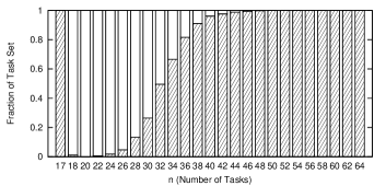
Figure 9: Fraction of task sets which requires 1 (crosshatch box) and 2 (empty box) reduction levels. 1000 task sets were generated for each point.

Figure 10: Distributions of the average number of preemptions per job, their quartiles, and their minimum and maximum values.

VI Related Work

Solutions to the real-time multiprocessor scheduling problem can be characterized according to the way task migration is controlled. Approaches which do not impose any restriction on task migration are usually called global scheduling. Those that do not allow task migration are known as partition scheduling. Although partition-based approaches make it possible using the results for uniprocessor scheduling straightforwardly, they are not applicable for task sets which cannot be correctly partitioned. On the other hand, global scheduling can provide effective use of a multiprocessor architecture although with possibly higher implementation overhead.

There exist a few optimal global scheduling approaches for the PPID model. If all tasks share the same deadline, it has been shown that the system can be optimally scheduled with a very low implementation cost [1]. Removing this restriction on task deadlines, optimality can be achieved by approaches that approximate the theoretical fluid model, according to which all tasks execute at the steady rate proportional to their utilization [2]. However, this fluid approach has the main drawback that it potentially generates an arbitrary large number of preemptions.

Executing all tasks at a steady rate is also the goal of other approaches [3, 12]. Instead of breaking all task in fixed-size quantum subtasks, such approaches define scheduling windows, called T-L planes, which are intervals between consecutive task deadlines. The T-L plane approach has been extended recently to accommodate more general task models [13]. Although the number of generated preemptions has shown to be bounded within each T-L plane, the number of T-L planes can be arbitrarily high for some task sets.

Other approaches which control task migration have been proposed [5, 14, 15, 6]. They have been called semi-partition approaches. The basic idea is to partition some tasks into disjunct subsets. Each subset is allocated to processors off-line, similar to the partition-based approaches. Some tasks are allowed to be allocated to more than one processor and their migration is controlled at run-time. Usually, these approaches present a trade-off between implementation overhead and achievable utilization, and optimality can be obtained if preemption overhead is not bounded.

The approach presented in this paper lie in between partition and global approaches. It does not assign tasks to processors but to servers and optimality is achieved with low preemption cost. Task migration is allowed but is controlled by the rules of both the servers and the virtual schedule. Also, as the scheduling problem is reduced from multiprocessor to uniprocessor, well known results for uniprocessor systems can be used. Indeed, optimality for fixed-utilization task set on multiprocessor is obtained by using an optimal uniprocessor scheduler, maintaining a low preemption cost per task.

It has recently been noted that if a set with $m+1$ tasks have their total utilization exactly equal to $m$, then a feasible schedule of these tasks on $m$ identical processors can be produced [16]. The approach described here generalizes this result. The use of servers was a key tool to achieve this generalization. The concept of task servers has been extensively used to provide a mechanism to schedule soft tasks [17], for which timing attributes like period or execution time are not known a priori. There are some server mechanisms for uniprocessor systems which share some similarities with one presented here [18, 19]. To the best of our knowledge the server mechanism presented here is the first one designed with the purposes of solving the real-time multiprocessor scheduling problem.

VII Conclusion

An approach to scheduling a set of tasks on a set of identical multiprocessors has been described. The novelty of the approach lies in transforming the multiprocessor scheduling problem into an equivalent uniprocessor one. Simulation results have shown that only a few preemption points per job on average are generated.

The results presented here have both practical and theoretical implications. Implementing the described approach on actual multiprocessor architectures is among the practical issues to be explored. Theoretical aspects are related to relaxing the assumed task model, e.g. sporadic tasks with constrained deadlines. Further, interesting questions about introducing new aspects in the multiprocessor schedule via the virtual uniprocessor schedule can be raised. For example, one may be interested in considering aspects such as fault tolerance, energy consumption or adaptability. These issues are certainly a fertile research field to be explored.

References

- [1] R. McNaughton, “Scheduling with deadlines and loss functions,” Management Science, vol. 6, no. 1, pp. 1–12, 1959.
- [2] S. Baruah, N. K. Cohen, C. G. Plaxton, and D. A. Varvel, “Proportionate progress: A notion of fairness in resource allocation,” Algorithmica, vol. 15, no. 6, pp. 600–625, 1996.
- [3] H. Cho, B. Ravindran, and E. D. Jensen, “An optimal real-time scheduling algorithm for multiprocessors,” in 27th IEEE Real-Time Systems Symp., 2006, pp. 101–110.
- [4] G. Levin, S. Funk, C. Sadowski, I. Pye, and S. Brandt, “DP-FAIR: A simple model for understanding optimal multiprocessor scheduling,” in Euromicro Conf. on Real-Time Systems, 2010, pp. 3–13.
- [5] B. Andersson, K. Bletsas, and S. Baruah, “Scheduling arbitrary-deadline sporadic task systems on multiprocessors,” in 29th IEEE Real-Time Systems Symp., 2008, pp. 385–394.
- [6] E. Massa and G. Lima, “A bandwidth reservation strategy for multiprocessor real-time scheduling,” in 16th IEEE Real-Time and Embedded Technology and Applications Symp., april 2010, pp. 175 –183.
- [7] B. Andersson and K. Bletsas, “Sporadic multiprocessor scheduling with few preemptions,” in 20th Euromicro Conf. on Real-Time Systems, July 2008, pp. 243–252.
- [8] K. Bletsas and B. Andersson, “Notional processors: An approach for multiprocessor scheduling,” in 15th IEEE Real-Time and Embedded Technology and Applications Symp., April 2009, pp. 3–12.
- [9] C. L. Liu and J. W. Layland, “Scheduling algorithms for multiprogram in a hard real-time environment,” Journal of ACM, vol. 20, no. 1, pp. 40–61, 1973.
- [10] P. Emberson, R. Stafford, and R. I. Davis, “Techniques for the synthesis of multiprocessor tasksets,” in Proc. of 1st Int. Workshop on Analysis Tools and Methodologies for Embedded and Real-time Systems (WATERS 2010), 2010, pp. 6–11.
- [11] ——, “A taskset generator for experiments with real-time task sets,” http://retis.sssup.it/waters2010/data/taskgen-0.1.tar.gz, Jan. 2011.
- [12] K. Funaoka, S. Kato, and N. Yamasaki, “Work-conserving optimal real-time scheduling on multiprocessors,” in 20th Euromicro Conf. on Real-Time Systems, 2008, pp. 13–22.
- [13] S. Funk, “An optimal multiprocessor algorithm for sporadic task sets with unconstrained deadlines,” Real-Time Systems, vol. 46, pp. 332–359, 2010.
- [14] A. Easwaran, I. Shin, and I. Lee, “Optimal virtual cluster-based multiprocessor scheduling,” Real-Time Syst., vol. 43, no. 1, pp. 25–59, 2009.
- [15] S. Kato, N. Yamasaki, and Y. Ishikawa, “Semi-partitioned scheduling of sporadic task systems on multiprocessors,” in 21st Euromicro Conf. on Real-Time Systems, 2009, pp. 249–258.
- [16] G. Levin, C. Sadowski, I. Pye, and S. Brandt, “SNS: A simple model for understanding optimal hard real-time multi-processor scheduling,” Univ. of California, Tech. Rep., 2009.
- [17] J. W. S. Liu, Real-Time Systems. Prentice-Hall, 2000.
- [18] Z. Deng, J. W.-S. Liu, and J. Sun, “A scheme for scheduling hard real-time applications in open system environment,” in 9th Euromicro Workshop on Real-Time Systems, 1997, pp. 191–199.
- [19] M. Spuri and G. Buttazzo, “Scheduling aperiodic tasks in dynamic priority systems,” Real Time Systems, vol. 10, no. 2, pp. 179–210, 1996.