Instability of the topological order and localization of the edge states in HgTe quantum wells coupled to s-wave superconductor

Abstract

Using the microscopic tight-binding equations we derive the effective Hamiltonian for the two-layer hybrid structure comprised of the two-dimensional HgTe quantum well-based topological insulator (TI) coupled to the s-wave isotropic superconductor (SC) and show that it contains terms describing mixing of the TI subband branches by the superconducting correlations induced by the proximity effect. We find that the proximity effect breaks down the rotational symmetry of the TI spectrum. We show that the edge states not only acquire the gap, as follows from the standard theory, but can also become localized by the Andreev-backscattering mechanism in a small coupling regime. In a strong coupling regime the edge states merge with the bulk states, and the TI transforms into an anisotropic narrow-gap semiconductor.

I Introduction

A topological insulator (TI), a material in which the electronic spectrum possesses an energy gap in the bulk but has the special, so-called topologically protected, edge (surface) states falling into this gap, is one of the focal points of current condensed matter studies. Volkov_TI ; Zgang_rev ; rev1 ; rev2 Topological insulators hold high technological promise since due to the ability of their topologically protected edge states to carry nearly dissipationless current they can be utilized in integrated circuits. Thus the question how robust the edge states are with respect to hybridization with the electronic states in the leads has become one of the focal points of current TI-related research.

Three dimensional (3D) TI have the Dirac spectrum with the finite mass in the bulk while the spectrum of the surface states is massless.3DTh ; 3DTh1 ; 3Dexp ; 3Dexp0 ; 3Dexp1 ; 3Dexp2 ; Zgang_rev Two-dimensional (2D) TI has the gapless helical edge states.Volkov_TI ; kane-mele ; BHZ The surface states in 3D TI and the edge states in 2D TI are topologically protected and are robust against all time-reversal-invariant local perturbations.Zgang_rev It was shown experimentally that 2D TI-state appears in HgTe/CdTe quantum wells (QW).Konig ; 2Dexp The TI in three-dimensional (3D) materials was found in Bi_1-xSb_x, Bi₂Se₃ and so on.3Dexp ; 3Dexp0 ; 3Dexp1 ; 3Dexp2

Of special interest are the states that develop at the interface between a TI and an s-wave superconductor (SC), like, e.g., in Fig.  1, where the proximity effect generates a superconducting pairing. it was shown that at the interface of 3D TI coupled to s-wave superconductor $p_{x}+ip_{y}$-superconducting state appears but without time-reversal symmetry breaking.Fu Numerical calculations showed that the proximity of the superconductor leads to a significant renormalization of the original parameters of the effective model describing the surface states of a topological insulator.stanesku For 2D topological insulator coupled to s-wave superconductor it is known that the momentum-independent gap enters in the edge spectrum.gang ; gang1 ; gang2 ; Jiang ; Jiang1

Two-dimensional TIs have a unique property: their parameters can be tuned over wide ranges of their values by the appropriate choice of the QW width $d$.Konig In particular, the main parameter of 2D TI, the gap in the bulk spectrum, $M$, can be changed from zero up to room temperature energy scale. Phenomenological treatment of the proximity effect is based on the assumption that the gap $M$ in the bulk spectrum of TI is much larger than the characteristics energy of the induced superconducting correlations. Unfortunately numerical calculations do not give the answer how the spectrum of the TI-SC system develops in this regime.Jiang ; Jiang1 In what follows we will focus on the gaps $M$ of the order of the energy of superconducting correlations.

In this Paper we investigate the effect of superconducting correlations on the topologically protected edge states and the bulk spectrum in the 2D topological insulator brought into a contact with the SC layer, see Fig. 1, and show the emergence of the SC correlations in the TI similarly to what was observed in GaAs containing a two-dimensional electron gas.Takayanagi ; Batov Ordinarily, the effective Hamiltonian of the TI in question is constructed from the symmetry considerations, see e.g., Ref. gang, ; gang1, ; gang2, , and has the trivial structure of the induced superconducting potentials. We demonstrate that the symmetry reasons suggest the additional non-diagonal (in the subband space) terms in the Hamiltonian. Moreover, using the microscopic tight-binding equations we derive analytically the additional terms in the effective Hamiltonian of the TI describing coupling to the $s$-wave isotropic superconductor (SC) placed on top of it. These terms become especially important in the case where the bare gap parameter $M$ of the TI becomes comparable to the characteristic energy of the induced superconducting correlations. We show, further, that the interplay of the superconducting and “topological” interactions is essential and results in several effects, in particular, the collapse of the topological order in TI. We find that while “topologicaly protected” edge states can ensure undisturbed propagation of the charge (spin) carriers, superconducting correlations can block the edge current causing a peculiar localization effect.

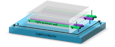
Figure 1: (Color online) Sketch of the 2D topological insulator coupled to a superconductor. The thick arrows show schematically the edge states.

On the qualitative level our results can be summarized as follows: in the absence of superconducting correlations the edge states spectrum is linear near the Fermi surface, comprising of two counter-propagating electron and two hole branches, respectively.Zgang_rev Importantly, the edge spectrum is isotropic in a sense that it does not depend on the orientation of the edges with respect to crystallographic axes, although the edge electronic states wave functions are orientation dependent. Namely, there is a phase difference between the wave function components corresponding to (E) or (H)-subbands in TI. The bulk spectrum is characterized by the gap $M$. At small SC-TI coupling (the quantitative criteria will be given below) the edge-states spectrum acquire a gap $E_{\mathrm{g}}$. Furthermore, superconducting correlations mix the subband branches and thus turn the resulting electronic spectrum in TI (edge and bulk), anisotropic, and $E_{\mathrm{g}}$ starts to depend on orientation of the edge. This can cause localization of the low-lying edge states since an inevitable bending of the edge will create the regions along the edge were the edge-particle energy $\varepsilon<E_{\mathrm{g}}$ thus getting locked between the turning points where $\varepsilon=E_{\mathrm{g}}$. At the turning points electron and hole excitations undergo Andreev reflection and form the localized Andreev bound edge states, see Fig. 2a. As the characteristic energy of the induced pairing amplitude exceeds $M$ then the gap of the continuum bulk states of TI collapses and TI behaves like the highly anisotropic narrow-gap semiconductor.

II Effective Hamiltonian

The low energy Hamiltonian of the two-dimensional (2D) topological insulator formed in the HgTe QW has the form:BHZ ; Zgang_rev

$$\operatorname{\check{\mathcal{H}}}=\begin{pmatrix}\hat{H}&0\\ 0&\hat{\tilde{H}}\\ \end{pmatrix},$$ (1)

where $\hat{H}=\epsilon_{k}+d_{i}\hat{\sigma}^{i}$, $i=\{1,2,3\}$; $\hat{\sigma}^{i}$ are the Pauli matrices acting in the subband (isospin) space; $\epsilon_{k}=C-Dk^{2}$. We choose the frame of reference so that $\vec{d}=(k_{x}A,-k_{y}A,M-Bk^{2})$. Here $A$, $B$, $C$, $D$ and $M$ are material parameters. The lower block of the Hamiltonian, $\hat{\tilde{H}}=\hat{\rho}^{T}\hat{H}^{*}\hat{\rho}=\epsilon_{k}-d_{i}(-k)\hat{\sigma}^{i}$, where $\hat{\rho}=i\hat{\sigma}_{y}$ is the metric tensor in the spinor space. The chosen representation for $\operatorname{\check{\mathcal{H}}}$ enables us to employ the machinery of the tensor bispinor algebra developed for Dirac Hamiltonian.

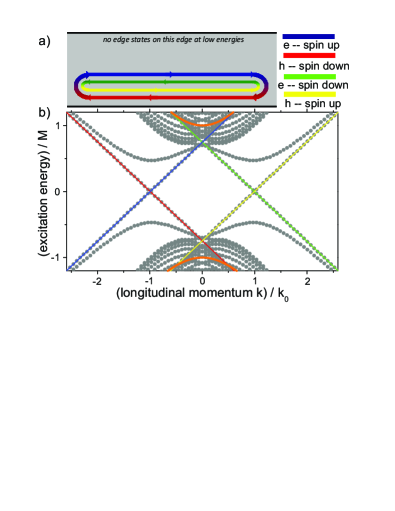
Figure 2: (Color online) a) A sketch of localized Andreev edge states in TI. b) Excitation spectrum in the 2D TI with proximity induced superconducting correlations: the edge modes at one TI-edge acquired the gap while the edge modes on the opposite edge remain gapless. Solid lines show the edge states and bulk spectrum boundaries in TI without superconducting correlations. The parameters are chosen as: $mk_{F}t_{a}^{2}/(2\pi\hbar^{2}M)=1$, $t_{b}=\sqrt{|B_{-}|/|B_{+}|}t_{a}$ and the orientation angle $\varphi=0$.

To construct the convenient form of the Bogoliubov – de Gennes (BdG) Hamiltonian describing superconductivity, we introduce the time reversal symmetry operator,

$$\check{\mathcal{T}}=\begin{pmatrix}0&0&0&-1\\ 0&0&1&0\\ 0&-1&0&0\\ 1&0&0&0\\ \end{pmatrix}{\mathcal{C}}=-\hat{\tau}_{1}\otimes i\hat{\sigma}_{2}\,\mathcal{C}\,,$$ (2)

where ${\mathcal{C}}$ is the operator of the complex conjugation and $\hat{\tau}_{i}$, are the Pauli matrices acting in spin space. Then the time-reverse of the BHZ-Hamiltonian (1) is $\check{\mathcal{T}}\operatorname{\check{\mathcal{H}}}\check{\mathcal{T}}^{-1}=\operatorname{\check{\mathcal{H}}}$. The BdG Hamiltonian is

$$\operatorname{{\mathcal{H}}_{\scriptscriptstyle{\mathrm{BDG}}}}=\begin{pmatrix}\operatorname{\check{\mathcal{H}}}+\operatorname{\check{\mathcal{U}}}&\check{\Delta}_{\rm\scriptscriptstyle TI}\\ \check{\Delta}^{+}_{\rm\scriptscriptstyle TI}&-\operatorname{\check{\mathcal{H}}}-\check{\mathcal{T}}\operatorname{\check{\mathcal{U}}}\check{\mathcal{T}}^{-1}\\ \end{pmatrix}\,,$$ (3)

where $\check{\Delta}_{\rm\scriptscriptstyle TI}$ is the effective proximity induced superconducting pairing matrix coupling the spin and subband spaces. The effective chemical potential shift appearing in the BCS theory has matrix form $\operatorname{\check{\mathcal{U}}}$. There is no reason to believe that the matrix structure of $\operatorname{\check{\mathcal{U}}}$ and $\check{\Delta}_{\rm\scriptscriptstyle TI}$ is necessary trivial like, e.g., in Ref. gang, ; gang1, ; gang2, ; symmetry considerations in fact allow nontrivial shape of theses matrices. So both, $\check{\Delta}_{\rm\scriptscriptstyle TI}$ and $\operatorname{\check{\mathcal{U}}}$ will be found below microscopically.

To proceed further we present the Hamiltonian describing the TI-SC coupling in a form:

$$H=H_{sc}+H_{2D}+H_{\rm int}\,.$$ (4)

The superconducting part is

$$H_{sc}=\sum\limits_{s=\uparrow,\downarrow}\int d^{3}r\Psi^{+}_{s}(\textbf{r})\left(\epsilon_{sc}-\mu\right)\Psi_{s}(\textbf{r})+\\ \int d^{3}r\left(\Delta\Psi^{+}_{\uparrow}(\textbf{r})\Psi^{+}_{\downarrow}(\textbf{r})+\Delta^{*}\Psi_{\downarrow}(\textbf{r})\Psi_{\uparrow}(\textbf{r})\right)$$ (5)

where, $\Psi_{\uparrow(\downarrow)}$ ($\Psi^{+}_{\uparrow(\downarrow)}$) are the field annihilation (creation) operators for the state with the spin up (down), $\Delta$ is the superconducting gap, $\epsilon_{sc}$ is the single electron kinetic energy, and $\mu$ is the Fermi energy.

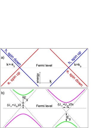
Figure 3: (Color online) The edge states at the TI boundary for a weak coupling where the edge states become gapped. a) Unperturbed edge-spectrum. b) Edge states with the proximity-induced gap. The shift of the zero point reflects the difference in the original chemical potentials.

The second quantization representation for the TI Hamiltonian is written in the basis of the Wannier functions for particles with spin $s$:

$$H_{2D,s}=\sum\limits_{\textbf{R}\textbf{R}^{\prime},s}\sum\limits_{\sigma,\sigma^{\prime}=a,b}c^{+}_{s\textbf{R},\sigma}\left(\epsilon_{2D,s}(\textbf{R}\sigma,\textbf{R}^{\prime}\sigma^{\prime})+\right.\\ \left.C\delta(\textbf{R},\textbf{R}^{\prime})\delta_{\sigma,\sigma^{\prime\prime}}\right)c_{s\textbf{R}^{\prime},\sigma^{\prime}}$$ (6)

where $\epsilon_{2D,s}(\textbf{R},\textbf{R}^{\prime})$ is the lattice representation of the BHZ-modelJiang ; Jiang1 (1) (see Appendix A). Then $H_{2D}=\sum_{s}H_{2D,s}$.

Finally, $H_{\rm int}$ reflects the electronic tunneling between the SC and TI:

$$H_{\rm int}=\sum\limits_{\textbf{R},s}\sum\limits_{\sigma=a,b}\left(t_{\sigma,\mathbf{R}}\Psi^{+}_{s}(\mathbf{R})c_{s\mathbf{R},\sigma}+t_{\sigma,\mathbf{R}}^{*}c^{+}_{s\mathbf{R},\sigma}\Psi_{s}(\mathbf{R})\right)\,,$$

where $c_{\uparrow(\downarrow)\textbf{R},a}$ is the superposition of $\left|\Gamma_{6},\pm\tfrac{1}{2}\right>$, $\left|\Gamma_{8},\pm\tfrac{1}{2}\right>$ and $c_{\uparrow(\downarrow)\textbf{R},b}$ refers to the subband $\left|\Gamma_{6},\pm\tfrac{3}{2}\right>$. Integrating out the bulk superconductor variables $\Psi_{s}(\mathbf{R})$ using the method, developed in Ref. Volkov, ; Meln_Kopnin_proxim_Delta, , one obtains the effective BdG-Hamiltonian (3) for the homogeneous tunneling amplitudes $t_{\sigma\textbf{R}}=t_{\sigma}$, with the matrix superconducting order parameter and the effective chemical potential shift having the form:

$$\check{\Delta}_{\rm\scriptscriptstyle TI}=\begin{pmatrix}\hat{\Delta}_{\rm\scriptscriptstyle TI}&0\\ 0&\hat{\tilde{\Delta}}_{\rm\scriptscriptstyle TI}\\ \end{pmatrix}\ ,\qquad\operatorname{\check{\mathcal{U}}}=\begin{pmatrix}\operatorname{\hat{\mathcal{U}}}&0\\ 0&\operatorname{\hat{\tilde{\cal U}}}\\ \end{pmatrix}\,.$$ (7)

Here

$$\hat{\Delta}_{\rm\scriptscriptstyle TI}=-\frac{mk_{F}}{2\pi\hbar^{2}}\begin{pmatrix}t_{a}^{*2}&t_{a}^{*}t_{b}^{*}\\ t_{a}^{*}t_{b}^{*}&t_{b}^{*2}\\ \end{pmatrix}\ ,\qquad\hat{\tilde{\Delta}}_{\rm\scriptscriptstyle TI}=\hat{\rho}^{T}\hat{\Delta}_{\rm\scriptscriptstyle TI}\hat{\rho}\,,$$ (8)

$$\operatorname{\hat{\mathcal{U}}}=\frac{m}{2\pi\hbar^{2}a_{\rm\scriptscriptstyle TI}}\begin{pmatrix}|t_{a}|^{2}&t_{a}^{*}t_{b}\\ t_{a}t_{b}^{*}&|t_{b}|^{2}\\ \end{pmatrix}\,,\qquad{\operatorname{\hat{\tilde{\cal U}}}}=\hat{\rho}^{T}\operatorname{\hat{\mathcal{U}}}\hat{\rho}\,,$$ (9)

$m$ and $k_{F}$ are the effective mass and the Fermi momentum of the bulk superconductor respectively, $a_{\rm\scriptscriptstyle TI}$ is the characteristic length scale of the order of the lattice constant in TI. Since $\Delta_{\scriptscriptstyle{\mathrm{TI}}}\ll\Delta$, the proximity induced parameters are independent of $\Delta$. Meln_Kopnin_proxim_Delta In Ref. gang, ; gang1, ; gang2, the potentials $\hat{\Delta}_{\rm\scriptscriptstyle TI}$ and $\operatorname{\hat{\mathcal{U}}}$ were diagonal (trivial) while the offdiagonal terms were missed.

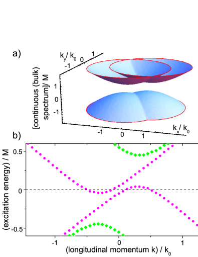
Figure 4: (Color online) Bulk and edge states for the intermediate coupling. a) Energy of the bulk states as function of $k_{x},k_{y}$. Without superconductivity, the bulk states dispersion is isotropic, $E(k)=\epsilon(k)\pm\sqrt{A^{2}k^{2}+(M-Bk^{2})^{2}}$,Zgang_rev where $k=\sqrt{k_{x}^{2}+k_{y}^{2}}$. Superconducting correlations make it anisotropic as follows from the noncommutativity of $\check{\Delta}$ and/or $\operatorname{\check{\mathcal{U}}}$ with $\operatorname{\check{\mathcal{H}}}$ in Eq.(3). b) Gapped edges states. The colors for the families of the dispersion curves are the same as in Fig. 3. The parameters are chosen as: $mk_{F}/(2\pi\hbar^{2})t_{a}^{2}/M=1$, $t_{b}=\sqrt{|B_{-}|/|B_{+}|}t_{a}\exp(i\pi/6)$ and the orientation angle $\varphi=\pi/2$.

For numerical calculations we take typical parameters: $A=3.8$ eVÅ, $B=-56.2$ eVŲ, $D=-38.7$ eVŲ. Without a loss of generality we take the energy-shift parameter $C=0$. We do not fix $M$ ($-10$meV$\lesssim M<0$) and use it as the energy unit. Our numerical and analytical calculations show the approximate symmetry relation that satisfies the spectrum of $\operatorname{{\mathcal{H}}_{\scriptscriptstyle{\mathrm{BDG}}}}$: $\chi E(\mathbf{k}/\chi,M/\chi,t_{a}/\sqrt{\chi},t_{b}/\sqrt{\chi})\approx E(\mathbf{k},M,t_{a},t_{b})$, where $\chi$ is a dimensionless scaling parameter. The scaling relation appears since $M$ is much smaller than the energy scales one can construct form $A$, $B$ and $D$. In addition, $M$ appears to be the most sensitive to the HgTe layer width: it changes with it by several orders of magnitude while the other parameters change by $\sim 20\%$ and their changes very slightly modify the spectrum.Zgang_rev

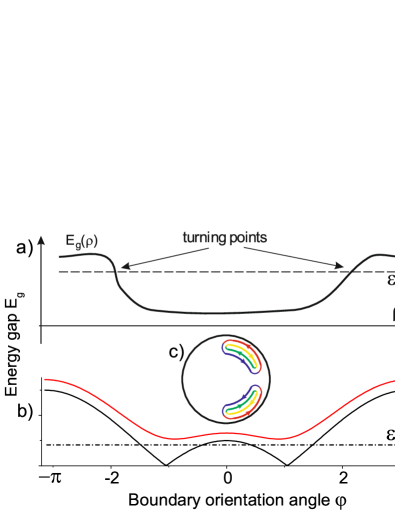
Figure 5: (Color online) Energy landscape for the edge states. a) Sketch of the energy landscape along the edge (parametrized by the coordinate $\rho$). The magnitude of the gap may change as a result of spatial fluctuations (like change in a shape of the TI boundary or fluctuations in tunneling amplitudes) and the state with the energy $\varepsilon$ would appear trapped between the turning points where $\varepsilon<E_{g}$ forming Andreev bound edge state like it is shown in Fig. 2. b) Calculated $E_{g}$ as function of the edge orientation angle $\varphi$ for the ratio $t_{a}/t_{b}\sqrt{|B_{-}/B_{+}|}\exp(-i\pi/3)$ equal to 1 (upper curve) and 2 (bottom curve). Such $E_{g}$ behavior can be observed in the sample shaped into a disc. c) Localized edge states in the sample shaped into a disc for energy $\epsilon$ corresponding to the dash-dot line in Fig. 5b.

First we discuss “weak” superconductivity where superconducting correlations induced in TI can be treated perturbatively. In this case matrix elements of $\check{\Delta}_{\rm\scriptscriptstyle TI}$ and $\operatorname{\check{\mathcal{U}}}$ are smaller than the gap in the continuum spectrum, $M$, in the bulk of TI. In the absence of superconducting correlations $\check{\Delta}_{\rm\scriptscriptstyle TI}=0$ and $\operatorname{\check{\mathcal{U}}}=0$, and there are two electron and two hole edge states at each TI surface. The edge states have the linear dispersion law with the velocity $s=A|\sqrt{B_{+}B_{-}}/B|$, where $B_{\pm}=B\pm D$. They cross the Fermi energy at $k=k_{0}=DM/(A\sqrt{B_{+}B_{-}})$ and $k=-k_{0}$, see Fig. 3a. We denote the wave functions of the electron and hole edge states near $k=k_{0}$ as $\psi^{(1)}=(\psi_{\rm edge},\hat{0},\hat{0},\hat{0})^{\tau}$ and $\psi^{(2)}=(\hat{0},\hat{0},\psi_{\rm edge},\hat{0})^{\tau}$, respectively, where $\hat{0}$ is the zero spinor in the subband space,

$$\psi_{\rm edge}=\frac{e^{-i\hat{\sigma}_{z}\varphi/2}}{\sqrt{2|B|}}\left(\sqrt{|B_{-}|}\atop-\sqrt{|B_{+}|}\right)\times\\ \left(e^{-\lambda_{+}\mathbf{r}\cdot\mathbf{n}}-e^{-\lambda_{-}\mathbf{r}\cdot\mathbf{n}}\right)e^{ik\mathbf{r}\cdot\mathbf{l}}\,,$$ (10)

$k$ is the momentum component parallel to the edge, $\mathbf{r}=(x,y)$, $\mathbf{l}$, and $\mathbf{n}$ are the unit vectors directed along the TI boundary and perpendicular to it correspondingly [$\mathbf{l}\times\mathbf{n}$ is aligned with the $OZ$ axis], and $\varphi$ is the angle between $\mathbf{l}$ and $OX$ axis. The decay length scales of the edge states into the bulk of the topological insulators are:

$$\lambda_{\pm}=\lambda_{0}\pm\sqrt{\left(k-\frac{D}{B}\lambda_{0}\right)^{2}+\frac{A^{2}}{4B^{2}}-\frac{M}{B}},$$ (11)

where $\lambda_{0}=A/(2\sqrt{B_{+}B_{-}})$. We stress that spinor components of $\psi_{\rm edge}$ depend on the TI-boundary orientation.

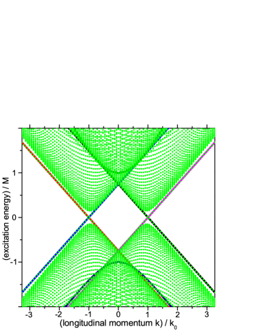
Figure 6: (Color online) Excitation spectrum in 2D TI for the proximity induced potentials being of the same order as the gap in TI in the absence of a SC. The gap between the branches of the continuum spectrum collapses and TI acquires metallic conductivity with the relativistic spectrum similar to that in graphene. Solid lines correspond to the edge states and the bulk spectrum boundaries in TI without superconducting correlations. Parameters are chosen as: $mkF/(2\pi\hbar^{2})t_{a}^{2}/M=12$, $\varphi=0$, and $t_{b}=\sqrt{|B_{-}|/|B_{+}|}t_{a}$.

The dispersion law of the edge states near $k=k_{0}$ within the perturbation theory taking in the account the superconducting correlations acquires the form:

$$\epsilon_{1,2}(k)=(\mathcal{U}_{11}+\mathcal{U}_{22}\pm\omega(k))/2,$$ (12)

where $\omega=\sqrt{(2s(k-k_{0})+\mathcal{U}_{11}-\mathcal{U}_{22})^{2}+4E_{g}^{2}}$; $\mathcal{U}_{ii}$, $i=1,2$ are the matrix elements of $\operatorname{\check{\mathcal{U}}}$ with respect to the states $\psi^{(1,2)}$ and $E_{g}=|(\check{\Delta}_{\rm\scriptscriptstyle TI})_{12}|$. They can be parameterized through $\mathcal{T}_{\pm}=\left|t_{a}\sqrt{|B_{-}|}-t_{b}\sqrt{|B_{+}|}e^{\pm i\varphi}\right|$. So,

$$E_{g}=\mathcal{T}_{+}\mathcal{T}_{-},$$ (13)

the matrix elements in the see Eq.(9) become $\operatorname{\check{\mathcal{U}}}_{11(22)}=\alpha\mathcal{T}_{+(-)}^{2}$, and $\alpha=(k_{F}a_{\rm\scriptscriptstyle TI})^{-1}$.

One now sees that the spectrum of the edge states becomes dependent upon the orientation of the boundary orientation with respect to crystallographic axis. This resembles the spectrum that often appear in the 3D TI which that are referred to as “strong” TI.stanesku

There is a wealth of the possible coupling-induced behaviours of the edge states energy spectrum. If $\mathcal{T}_{+}=0$ or $\mathcal{T}_{-}=0$, then $E_{g}=0$ as well; the situation where $E_{g}$ is very small is also common. A particular picture depends on the edge orientation angle $\varphi$ and/or on the tunneling amplitudes, $t_{a}$ and $t_{b}$. Shown in the Fig. 2 is the situation where at one boundary of the TI-strip the edge states remain gapless ($E_{g}=0$) while at the opposite boundary $E_{g}\neq 0$ and the edge states have the gap. The stripe within which the edge states are confined has a finite length (see in Fig. 2), there are points at the edge where the TI-boundary changes its direction and, at the same time, the value of $E_{g}$ changes. At these “turning points” electron and hole edge (going in the opposite direction) states with the energy smaller than $E_{g}$ undergo the Andreev reflection and form the bound Andreev edge state, see Figs. 2,5. Illustrated in Figs. 3-4 is the structure of the the edge state energy levels in the case where $E_{g}$ is finite.

Now we discuss a general nonperturbative situation. The excitation spectrum in 2D TI accounting for the proximity induced superconducting correlations in the case where proximity induced potentials in TI are of the same order as the gap in TI without superconductor on top is shown in Fig. 6. The gap between the branches of the continuum spectrum nearly closes and TI acquires effectively metallic conductivity with the relativistic spectrum similar to that in graphene. Solid lines correspond to the edge states and bulk spectrum boundaries in TI without superconducting correlations.

III Conclusions

To conclude, we investigated topologically protected edge states in QW of HgTe sandwiched between CdTe and demonstrated that the $s$-wave isotropic superconductor placed on top of CdTe layer induces superconducting correlations in the TI revealing the built in anisotropy of TI which did not affect the spectrum when superconducting correlations were absent. The form of the edge states spectrum essentially depends on the edge orientation with respect to crystallographic directions of the TI. Depending on the coupling between the superconductor and 2D TI, different scenarios can be realized: (i) the edge states of the topological insulator acquire a gap, (ii) the edge states hybridize into the Andreev localized edge state and/or (iii) the gap separating the continuum and the edge modes collapses and TI becomes the narrowgap (anisotropic) semiconductor. Our predictions can be verified by means of, for example, scanning tunnelling spectroscopy measurements of the spectra showed in Fig. 3 where the shift of the zero point $U_{11}+U_{22}$ can be tuned by the gate placed on top of the CdTe layer.

Note: After this work has been completed we became aware of the recent experiments on InAs/GaSb QW.2DexpAS which revealed the 2D TI state.2DexpAS Since this novel TI is expected to be well described by the BHZ-model, our results apply to InAs/GaSb QW coupled to s-wave superconductor as well.

IV Acknowledgments

This work was supported by the U.S. Department of Energy Office of Science under the Contract No. DE-AC02-06CH11357, the work of IMK and NMC was partly supported by the Russian president foundation (mk-7674.2010.2) under the Federal program “Scientific and educational personnel of innovative Russia”.

Appendix A Lattice model

Microscopic description of the coupling between TI and the superconductor developed on the base of the standard lattice regularization of the BHZ-model (1) replacing its parameters by:Zgang_rev

$$\epsilon_{k}=C-2Da^{-2}\left[2-\cos k_{x}a-\cos k_{y}a\right],$$ (14)

$$\vec{d}=\left(Aa^{-1}\sin k_{x}a,-Aa^{-1}\sin k_{y}a,M-Ba^{-2}\left[2-\cos k_{x}a-\cos k_{y}a\right]\right).$$ (15)

This corresponds to the quadratic Bravais lattice (with the translation vectors $\textbf{a}_{1}=a\textbf{x}_{0}$, $\textbf{a}_{2}=a\textbf{y}_{0}$) with two type of states (corresponding annihilation operators are $\hat{c}_{a\textbf{R}}$ and $\hat{c}_{b\textbf{R}}$) on each site replying to subband states. Therefore the Hamiltonian describing TI in the second quantization representation in the basis of the Wannier functions for particles with spin $s$, takes the form:

$$\hat{H}_{2D,s}=\sum\limits_{\textbf{R}\textbf{R}^{\prime},s}\sum\limits_{\sigma,\sigma^{\prime}=a,b}\hat{c}^{+}_{s\textbf{R},\sigma}\left(\hat{\epsilon}_{2D,s}(\textbf{R}\sigma,\textbf{R}^{\prime}\sigma^{\prime})+C\delta(\textbf{R},\textbf{R}^{\prime})\delta_{\sigma,\sigma^{\prime\prime}}\right)\hat{c}_{s\textbf{R}^{\prime},\sigma^{\prime}}\ ,$$ (16)

where

$$\hat{\epsilon}_{2D,s}(\textbf{R}\tilde{\sigma},\textbf{R}^{\prime}\tilde{\sigma}) =\delta_{\textbf{R}\textbf{R}^{\prime}}\left[\left(M-\frac{4B}{a^{2}}\right)\tilde{\sigma}-\frac{4D}{a^{2}}\right]+\left(\frac{4B}{a^{2}}\tilde{\sigma}+\frac{4D}{a^{2}}\right)\left(\delta_{\textbf{R+a}_{1},\textbf{R}^{\prime}}+\delta_{\textbf{R-a}_{1},\textbf{R}^{\prime}}+\delta_{\textbf{R+a}_{2},\textbf{R}^{\prime}}+\delta_{\textbf{R-a}_{2},\textbf{R}^{\prime}}\right)$$ (17a)

$$\hat{\epsilon}_{2D,\uparrow}(\textbf{R}a,\textbf{R}^{\prime}b) =-\hat{\epsilon}_{2D,\downarrow}(\textbf{R}b,\textbf{R}^{\prime}a)=\frac{A}{2a}\left(\delta_{\textbf{R+a}_{2},\textbf{R}^{\prime}}-\delta_{\textbf{R-a}_{2},\textbf{R}^{\prime}}-i\delta_{\textbf{R+a}_{1},\textbf{R}^{\prime}}+i\delta_{\textbf{R-a}_{1},\textbf{R}^{\prime}}\right)$$ (17b)

$$\hat{\epsilon}_{2D,\uparrow}(\textbf{R}b,\textbf{R}^{\prime}a) =-\hat{\epsilon}_{2D,\downarrow}(\textbf{R}a,\textbf{R}^{\prime}b)=-\hat{\epsilon}^{*}_{2D,\uparrow}(\textbf{R}a,\textbf{R}^{\prime}b)\,.$$ (17c)

References

- (1) B. A. Volkov and O. A. Pankratov, JETP Lett. 42, 178 (1985).
- (2) X. L. Qi, S. C. Zhang, arXiv:1008.2026v1.
- (3) J. E. Moore, Nature (London) 464, 194 (2010).
- (4) M. Z. Hasan and C. L. Kane, Rev. Mod. Phys. 82, 3045 (2010).
- (5) L. Fu, C. L. Kane, and E. J. Mele, Phys. Rev. Lett. 98, 106803 (2007).
- (6) H. Zhang, C.-X. Liu, X.-L. Qi, X. Dai, Z. Fang, and S.-C. Zhang, Nat. Phys. 5, 438 (2009).
- (7) D. Hsieh, D. Qian, L. Wray, Y. Xia, Y. S. Hor, R. J. Cava, and M. Z. Hasan, Nature (London) 452, 970 (2008).
- (8) D. Hsieh, Y. Xia, D. Qian, L. Wray, J. H. Dil, F. Meier, J. Osterwalder, L. Pattey, J. G. Checkelsky, N. P. Ong, A. V. Fedorov, H. Lin, A. Bansil, D. Grauer, Y. S. Hor, R. J. Cava, and M. Z. Hasan, ibid. 460, 1101 (2009).
- (9) Y. L. Chen, J. G. Analytis, J.-H. Chu, Z. K. Liu, S.-K.Mo, X. L. Qi, H. J. Zhang, D. H. Lu, X. Dai, Z. Fang, S. C. Zhang, I. R. Fisher, Z. Hussain, and Z.-X. Shen, Science 325, 178 (2009).
- (10) T. Zhang, P. Cheng, X. Chen, J.-F. Jia, X. Ma, K. He, L. Wang, H. Zhang, X. Dai, Z. Fang, X. Xie, and Q.-K. Xue, Phys. Rev. Lett. 103, 266803 (2009).
- (11) C. L. Kane and E. J. Mele, Phys. Rev. Lett. 95, 146802 (2005); 95, 226801 (2005).
- (12) B. A. Bernevig, T. L. Hughes, and S-C. Zhang, Science 314, 1757 (2006).
- (13) M. Konig, S. Wiedmann, C. Brune, A. Roth, H. Buhmann, L. W. Molenkamp, Xiao-Liang Qi, and S.-C. Zhang, Science 318, 766 (2007).
- (14) A. Roth, C. Brüne, H. Buhmann, L.W. Molenkamp, J. Maciejko, X.-L. Qi, and S.-C. Zhang, Science 325, 294 (2009).
- (15) L. Fu and C.L. Kane, Phys. Rev. Lett. 100, 096407 (2008).
- (16) T.D. Stanescu, J.D. Sau, R.M. Lutchyn, and S. Das Sarma, Phys. Rev. B 81, 241310(R) (2010).
- (17) Liang Fu and C.L. Kane, Phys. Rev. B 79, 161408(R) (2009).
- (18) J. Nilsson, A.R. Akhmerov, and C.W.J. Beenakker, Phys. Rev. Lett. 101, 120403 (2008).
- (19) P. Adroguer, C. Grenier, D. Carpentier, J. Cayssol, P. Degiovanni, and E. Orignac, Phys. Rev. B 82, 081303(R) (2010).
- (20) Hua Jiang, Lei Wang, Qing-feng Sun, and X.C. Xie, Phys. Rev. B 80, 165316 (2009).
- (21) Qing-Feng Sun, Yu-Xian Li, Wen Long, and Jian Wang, Phys. Rev. B 83, 115315 (2011).
- (22) H. Takayanagi, T. Akazaki, and J. Nitta, Phys. Rev. Lett. 75, 3533 (1995).
- (23) I.E. Batov, T. Schäpers, N.M. Chtchelkatchev, H. Hardtdegen, and A.V. Ustinov, Phys. Rev. B 76, 115313 (2007).
- (24) A.F. Volkov, P.H.C. Magnee, B.J. van Wees, and T.M. Klapwijk, Physica C 242, 261 (1995).
- (25) A. S. Mel’nikov, N. B. Kopnin, arXiv:1105.1903.
- (26) I. Knez, R.R. Du, and G. Sullivan, arXiv:1105.0137; ibid, arXiv:1106.5819v1.