Clean relaying aided cognitive radio under the coexistence constraint

Abstract

We consider the interference-mitigation based cognitive radio where the primary and secondary users can coexist at the same time and frequency bands, under the constraint that the rate of the primary user (PU) must remain the same with a single-user decoder. To meet such a coexistence constraint, the relaying from the secondary user (SU) can help the PU’s transmission under the interference from the SU. However, the relayed signal in the known dirty paper coding (DPC) based scheme is interfered by the SU’s signal, and is not “clean”. In this paper, under the half-duplex constraints, we propose two new transmission schemes aided by the clean relaying from the SU’s transmitter and receiver without interference from the SU. We name them as the clean transmitter relaying (CT) and clean transmitter-receiver relaying (CTR) aided cognitive radio, respectively. The rate and multiplexing gain performances of CT and CTR in fading channels with various availabilities of the channel state information at the transmitters (CSIT) are studied. Our CT generalizes the celebrated DPC based scheme proposed previously. With full CSIT, the multiplexing gain of the CTR is proved to be better (or no less) than that of the previous DPC based schemes. This is because the silent period for decoding the PU’s messages for the DPC may not be necessary in the CTR. With only the statistics of CSIT, we further prove that the CTR outperforms the rate performance of the previous scheme in fast Rayleigh fading channels. The numerical examples also show that in a large class of channels, the proposed CT and CTR provide significant rate gains over the previous scheme with small complexity penalties.

I Introduction

Efficient spectrum usage becomes a critical issue to satisfy the increasing demands for high data rate services. Recent measurements from the Federal Communications Commission (FCC) have indicated that ninety percent of the time, many licensed frequency bands remain unused and are wasted. Cognitive radio [1] is a promising technique to cope with such problems by accessing the unused spectrum dynamically. This new technology is capable of dynamically sensing and locating unused spectrum segments in a target spectrum pool, and communicating via the unused spectrum segments without causing harmful interference to the primary users. The primary user (PU) is the user who communicates in the licensed band using existing commercial standards, while the user who uses the cognitive radio technology is called the secondary user (SU). Originally, the cognitive radio adopts the interference avoidance methodology, that is, if a PU demands the licensed band, the SU should vacate and find an alternative one. Recently, the concept of interference mitigation was proposed for the cognitive radio [2], where the SU and PU can coexist and simultaneously transmit at the same time and frequency bands to further improve the spectrum efficiency. The key is to allow cooperations between the transmitters of the SU and PU. To make the interference-mitigation based cognitive radio in [2] more practical, the coexistence constraint was further proposed in [3]. The cognitive radio is forced to maintain the same PU rate performance as if it is silent, under the constraint that the decoder of PU must be a single-user decoder, such as the conventional minimum distance decoder. Assuming that the PU’s message is known by the SU, in [3], the SU’s transmitter not only transmits its own signal but also relays the PU’s signal to meet the coexistence constraint. Moreover, by precoding with the celebrated dirty paper coding (DPC) [4], the SU’s receiver can decode as if the interference from the PU does not exist. Indeed, such a transmission scheme is proved to be capacity-achieving in some channel conditions [3].

However, there are still some deficiencies and impractical assumptions in the cognitive radio proposed in [3] which motivate our work. First, in [3], the relayed PU’s signal and the SU’s own signal are simultaneously transmitted. Since the SU’s signal is an interference to the PU’s receiver, it pollutes the relaying and may cause power inefficiency. Second, the DPC requires that the SU’s transmitter knows the PU’s message. It may be hard to satisfy this requirement, especially when the channel between the transmitters of the PU and SU is not good enough. Finally, the perfect channel state information at the transmitter (CSIT) may not always be available, epically when the channel is fast faded. Without full CSIT, the DPC used in [3] suffers [5]. To solve these problems, we propose two new transmission schemes for cognitive radio which are aided by the “clean” relaying to the PR’s receiver without the interference from the SU. Under the half-duplex constraint, the clean relaying comes from the transmitter or/and the receiver of SU, thus we name the proposed schemes as the clean transmitter relaying (CT) and the clean transmitter-receiver relaying (CTR) aided cognitive radio, respectively.

Our main contributions are proposing the new CT and CTR to improve the performance in [3]. Our CT generalizes the DPC-precoded cognitive radio in [3]. Moreover, our CTR can also avoid the last two problems mentioned in the previous paragraph since it does not require the DPC. The cooperation method of the CTR makes it face a multiple-access channel (MAC) with common message, and we adopt the optimal signaling for this channel from [6] in the CTR. We also invoke the channel coding theorem in [7] to ensure that the coexistence constraint is met under the relaying. With full CSIT and high signal-to-noise ratio (SNR), we find that the multiplexing gain performance of the CTR is better than (or at least no less than) that of [3]. This is due to the fact that the silent period spent on decoding the PU’s messages for the DPC in [3] may not be necessary in the CTR. When there is only the statistics of CSIT, the CTR is even more promising. We observe that the DPC used in [3] fails in fast Rayleigh fading channels, that is, the rate performance of the SU is the same as that of treating the interference from the PU as pure noise at the SU’s receiver. Then the CTR always has better rate performance than that of [3] for all SNR regimes. We also identify the structure of the optimal common message relaying ratio for the CTR by exploring the corresponding stochastic rate optimization problem. Simulation results verify the superiority of the proposed CT and CTR over methods in [3] in terms of rates and multiplexing gains under a large class of channels. Finally, the complexity of the CTR is lower than that in [3], while the complexity of the CT is approximately the same as that in [3]. The former is because the signaling from [6] adopted in the CTR is much easier to implement in practice than the complicated DPC [8].

The cognitive channel model studied in the paper is related to [9][10], where cooperations in interference channels were studied. However, the coexistence constraints were not imposed in these papers, and thus the relay strategies could be more flexible to obtain better rate performance compared with ours. As noted in [3], the capacity results for these less restricted channels can serve as the performance outer bounds for our setting. Moreover, full CSIT is usually assumed in the literatures [2][3][9][10] (also in our previous work [11]), while this work also considers the partial CSIT case. With only the statistics of CSIT, we show that our CTR outperforms the DPC based schemes in [3][5] in fast Rayleigh fading channels. In addition, the CT and multiplexing gain analysis also are new, and did not appear in our previous works [11].

The paper is organized as following. The system model is discussed in Sec. II. In Sec.III and IV, we present the proposed CT and CTR and their rate and multiplexing gain performances with full CSIT, respectively. The performance analysis and the optimal common message relaying ratio with only the statistics of CSIT in fast Rayleigh fading channels are given in Sec. V. We provide numerical examples in Sec. VI. Finally, Sec. VII concludes this paper.

II System Model

II-A Notations

In this paper, the superscript $(.)^{H}$ denotes the transpose complex conjugate. Identity matrix of dimension $n$ is denoted by $\mathbf{I}_{n}$. A block-diagonal matrix with diagonal entries $\mathbf{A}_{1},\ldots,\mathbf{A}_{k}$ is denoted by $diag(\mathbf{A}_{1},\ldots,\mathbf{A}_{k})$; while $|\mathbf{A}|$ and $|a|$ represent the determinant of a square matrix $\mathbf{A}$ and the absolute value of a scalar variable $a$, respectively. The mutual information between two random variables is denoted by $I(;)$. We define $C(x)\triangleq\log(1+x)$ (the base of $\log$ function is 2), and the function $(x)^{+}$ as $(x)^{+}=x$ if $x\geq 0$, otherwise, $(x)^{+}=0$. Also the indicating function $\mathbf{1}_{A}$ is one if the event $A$ is valid, and is zero otherwise.

II-B Cognitive channel model

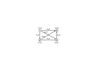
Figure 1: Cognitive channel model, where the TX and RX are the abbreviations of the transmitter and receiver, respectively.

As shown in Fig. 1, in the considered four-node cognitive channel, Node 1 and 2 are the transmitters of PU and SU while Node 4 and 3 are the corresponding receivers, respectively. For the $t$-th symbol time where $t$ is the discrete time index, the received signals $Y_{2}(t)$, $Y_{3}(t)$ and $Y_{4}(t)$ at Node 2, 3 and 4 can be respectively represented by

$$\left[\begin{array}[]{c}Y_{4}(t)\\ Y_{3}(t)\\ Y_{2}(t)\end{array}\right]=\left[\begin{array}[]{ccc}h_{14}(t)&h_{24}(t)&h_{34}(t)\\ h_{13}(t)&h_{23}(t)&0\\ h_{12}(t)&0&0\end{array}\right]\left[\begin{array}[]{c}X_{1}(t)\\ X_{2}(t)\\ X_{3}(t)\end{array}\right]+\left[\begin{array}[]{c}Z_{4}(t)\\ Z_{3}(t)\\ Z_{2}(t)\end{array}\right],$$ (1)

where the channel gain between node $i$ and $j$ is denoted by $h_{ij}(t)$, and $Z_{i}(t)$ is the additive white Gaussian noise process at node $i$. Each time sample of $Z_{i}(t)$ is independent and identically distributed (i.i.d.) circularly-symmetric complex Gaussian, i.e., $Z_{i}\sim\mathcal{CN}(0,1)$. Signals transmitted from Node 1, 2 and 3 are denoted as $X_{1}(t)$, $X_{2}(t)$, and $X_{3}(t)$ with long term average power constraints $\bar{P}_{1}$, $\bar{P}_{2}$, and $\bar{P}_{3}$, respectively as

$$\frac{1}{n}\sum^{n}_{t=1}[|X_{i}(t)|^{2}]\leq\bar{P}_{i},\;\;\mathrm{for}\;\;i=1,\,2,\,3,$$ (2)

where $n$ is the number of coded symbols in a codeword. Note that all nodes are half-duplex.

In this paper, we consider two cases with different channel knowledge of $h_{ij}(t)$ at the transmitter, while the channel gains $h_{ij}(t)$ are always assumed perfectly known at the corresponding receivers. In the first case, $h_{ij}(t)=h_{ij}=|h_{ij}|e^{j\theta_{ij}},\;\;\forall 1\leq t\leq n$, where $\theta_{ij}$ is the channel phase. As for the CSIT assumptions, we assume that Node 1 knows $h_{14}$, Node 3 knows $h_{34}$, and Node 2 knows all channel gains based on the method proposed in [3]. The second case is the fast Rayleigh fading channel, where each $h_{ij}(t)$ is varying at each $t$. We assume that $h_{ij}(t)$ are i.i.d. generated according to a random variable $H_{ij}$, and $H_{ij}$ is complex Gaussian distributed with zero mean and variance $\sigma^{2}_{ij}$. Moreover, due to the limited channel feedback bandwidth, we assume that the channel realizations $h_{ij}(t)$ are unknown at the transmitters. However, Node 1 knows the statistics of $H_{14}$, Node 3 knows the statistics of $H_{34}$, and Node 2 knows the statistics of all channels by applying the methods in [5][3]. The SU also knows the target rate of the PU by using the methods in [5, Sec. II].

We restrict the decoder of PU at Node 4 as a single-user decoder. A single-user decoder $D_{s}$ is defined to be any decoder which performs well on the point-to-point channel with perfect channel state knowledge at the decoder [3]. Without loss of generality, we set the decoder to be the maximum-likelihood decoder for fading channel with temporal independent Gaussian noise as in [12] (minimum-distance decoder). We then define the achievable rate under such decoder as the following.

Definition 1

A rate $R_{1}$ is single-user achievable for the PU if there exists a sequence of $(2^{nR_{1}},n)$ encoders $E^{n}_{1}$ that encodes PU’s message $w_{1}$, such that the average probability of error vanishes to zero as $n\rightarrow\infty$ when the receiver uses a single user decoder $D_{s}$.

Denote the set of all primary encoders that map primary messages to the transmitted signals as $E^{n}_{1}$ , we then have the following definition.

Definition 2

A cognitive radio code with rate $R_{2}$ and length $n$ consists of an encoder to encode the SU’s message $w_{2}$ with output $X^{n}_{2}=\{X_{2}(1),\ldots,X_{2}(n)\}$ as $E^{n}_{2}:E^{n}_{1}\times\{1,\ldots,2^{nR_{1}}\}\times\{1,\ldots,2^{nR_{2}}\}\rightarrow X^{n}_{2},$ where $\|X^{n}_{2}\|^{2}/n\leq\bar{P}_{2}$, and a decoder to decode message $w_{2}$ from the received signal $Y^{n}_{3}=\{Y_{3}(1),\ldots,Y_{3}(n)\}$.

Based on Definition 2, we have the following definition for the achievable rate of the cognitive radio under the coexistence constraint [3] .

Definition 3

The coexistence constraint means that for a given PU’s rate $R_{T}$, the SU must take $R_{T}$ as a rate target and ensure that under its own transmissions, $R_{T}$ is still single-user achievable for the PU as defined in Definition 1. A rate $R_{2}$ is achievable for the SU if there exists a sequence of $(2^{nR_{2}},n)$ cognitive radio codes defined in Definition 2 such that under the coexistence constraint, the average probability of error vanishes to zero as $n\rightarrow\infty$.

III Clean Transmitter Relaying in Channels with Full CSIT

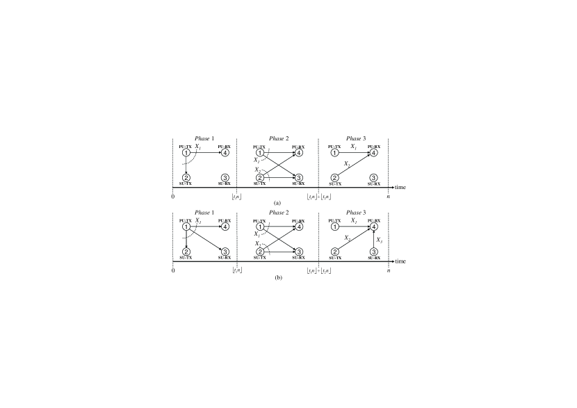
Figure 2: The signaling methods of the (a) CT and (b) CTR aided cognitive radio.

For simplicity, we will introduce the CT aided cognitive radio and its performance in channels with full CSIT first. Then we will discuss the CTR which further allows the relaying from the SU’s receiver in Section IV. As shown in Fig. 2 (a), the new three-phase CT is a generalization of the two-phase cognitive radio in [3], by introducing an additional “clean” relay link (without interference from the SU) from Node 2 in the third phase. As will be shown later, to know the PU’s message $w_{1}$ for the DPC operation, Node 2 needs Phase 1 to be long enough to correctly decode $w_{1}$ from the received signal. However, this phase is neglected in [3] and most of the existing works. It is also clear from Fig. 2 (a) that due to the half-duplex constraint, the transmission scheme must be multi-phase since Node 2 cannot receive and transmit at the same time. As will be clarified later, the multi-phase transmission will cause SNR changes at Node 4 in different phases. To deal with this new problem, we need to invoke the upcoming Lemma 1 to meet the coexistence constraint.

The detailed CT signaling method of each phase in Fig. 2 (a) comes as the following. To simplify the notations, we omit the time index of the signals in (1) to represent the corresponding signals in the Shannon random coding setting [13]. For example, $X_{1}$ corresponds to $X_{1}(t)$. Assume that each three-phase transmission occupies $n$ symbol times, which forms a codeword. We have

Phase 1: Within the first $\lfloor t_{1}n\rfloor$ symbols, Node 2 listens to and decodes the PU’s message $w_{1}$. Here $t_{i}$ is the portion of time of Phase $i$, $i=1,2,3$.

Phase 2: If the decoding of $w_{1}$ is successful, within the next $\lfloor t_{2}n\rfloor$ symbols, Node 2 sends the DPC encoded signal $X^{D}_{2}$ using side-information $h_{13}X_{1}$ plus the relaying of $X_{1}$ as

$$X_{2}=X^{D}_{2}+\sqrt{\alpha_{1}\frac{P_{2}}{P_{1}}}e^{j(\theta_{14}-\theta_{24})}X_{1},$$ (3)

where message $w_{2}$ is conveyed in $X^{D}_{2}$, $\alpha_{1}$ is the relay ratio from Node 2 to maintain the rate performance $R_{T}$ of the primary link, while $P_{1}$ and $P_{2}$ are the transmitted power of $X_{1}$ and $X_{2}$ in Phase 2, respectively.

Phase 3: For the remaining $t_{3}n=n-\lfloor t_{1}n\rfloor-\lfloor t_{2}n\rfloor$ symbols, the clean relaying is transmitted from Node 2 to assist decoding at Node 4 as

$$X_{2}=\sqrt{P_{2}/P_{1}}{\rm e}^{j(\theta_{14}-\theta_{24})}X_{1}.$$ (4)

To meet average power constraints (2), the power $P_{1}$ and $P_{2}$ are set as

$$P_{1}=\bar{P}_{1}\;\;\mbox{and}\;\;(1-t_{1})P_{2}=\bar{P}_{2}.$$ (5)

After Phase 1, Node 2 knows the PU’s message $w_{1}$. Since Node 2 also knows the PU’s codebook from Definition 2, the PU’s transmitted codeword and then the interference at Node 3 $h_{13}X_{1}$ is known at Node 2. The DPC results in [4] can be applied by using $h_{13}X_{1}$ as the non-causally known transmitter side-information which is unknown at Node 3.

Note that the received SNR of $X_{1}$ at Node 4 changes in different phases (different block of symbols). To meet the coexistence constraint in Definition 3 under this phenomena, we introduce a Lemma as

Lemma 1

For a block of $n$ transmissions over the channel $Y^{n}={\mathbf{H}}^{n}X^{n}+Z^{n}$, where $n\times 1$ vectors $X^{n}$ and $Y^{n}$ are the transmit and received signals respectively, the diagonal channel matrix ${\mathbf{H}}^{n}$ is known at the receiver, and $Z^{n}$ is a Gaussian random sequence with diagonal covariance matrix $K_{Z^{n}}$ (each element of $Z^{n}$ may not be identically distributed), the coding rate $R$ is single-user achievable for Gaussian codebooks if

$$R<\frac{1}{n}\log\frac{|{\mathbf{H}}^{n}K_{X^{n}}({\mathbf{H}}^{n})^{H}+K_{Z^{n}}|}{|K_{Z^{n}}|},$$ (6)

where the covariance matrix $K_{X^{n}}$ of the transmitted signal $X^{n}$ satisfies the power constraint.

In Lemma 1, the $n\times n$ channel matrix ${\mathbf{H}}^{n}$ is a collection of scalar time-domain channel coefficients over the $n$ transmissions. It is different to the spatial-domain channel matrix over single transmission in the multiple-antenna system [14], where the vector channels are assumed to be i.i.d in time. The proof of this lemma follows the steps in [7] where the asymptotic equipartition property for arbitrary Gaussian process is invoked to prove that the right-hand-side (RHS) of (6) is achievable by the suboptimal jointly typical decoder. Then it is also achievable by the optimal maximum-likelihood decoder defined in Definition 1. The detail is omitted. Then we have the following achievable rate result for the CT with the proof given in Appendix -A

Theorem 1

With full CSIT and the transmitted power setting in (5), the following rate of SU is achievable by the CT

$$R_{2}\leq\max_{t_{2},\alpha_{1}}\;\;t_{2}C(|h_{23}|^{2}(1-\alpha_{1})P_{2}),$$ (7)

which is subject to the constraint for coexistence with

$$R_{T}<t_{1}C(|h_{14}|^{2}P_{1})+t_{2}C\left(\frac{(|h_{14}|\sqrt{P_{1}}+|h_{24}|\sqrt{\alpha_{1}P_{2}})^{2}}{1+|h_{24}|^{2}(1-\alpha_{1})P_{2}}\right)+(1-t_{1}-t_{2})C\left(\left(|h_{14}|\sqrt{P_{1}}+|h_{24}|\sqrt{P_{2}}\right)^{2}\right),$$ (8)

and the constraint for Node 2 to successfully decode PU’s message as

$$t_{1}>R_{T}/C(|h_{12}|^{2}P_{1}),$$ (9)

where the intervals of Phase 1 and 2 are $\lfloor t_{2}n\rfloor$ and $\lfloor t_{2}n\rfloor$, respectively, and the relaying ratio $\alpha_{1}\in[0,1]$.

Note that in [3], there is no Phase 3 ($t_{3}=0$) and the relaying from SU is always “noisy” (interfered by SU’s own signal $X^{D}_{2}$) from (3). When the channel gain $|h_{24}|$ is large, much of the SU’s available power are used to overcome the interference from SU’s own signal and the transmission may not be efficient ($\alpha_{1}$ is high). Also in [3], the assumption $|h_{12}|\gg|h_{14}|$ or $I(X_{1};Y_{2})\gg R_{T}$ is made to ensure that $t_{1}$ can be essentially neglected ($t_{2}=1$), and the SNR is almost the same within a codeword. Thus the conventional Shannon channel coding theorem in [13] can be invoked to ensure the coexistence constraint. However, we usually have $t_{1}\neq 0$ for any more reasonable channel setting. Then the SNRs of Phase 1 and 2 are different at Node 4, that is, SNR changes in different block of symbols. The Lemma 1, which is more general than that in [13], is required to ensure that the PU’s rate is single-user achievable in Definition 1. The insight of this Lemma is that even when Node 4 encounters bad SNR at Phase 1, we can boost the SNR in Phase 2 to make the rate over all phases unchanged. Note that since the equivalent channel and noise change in different phases in the CT (also in its special case where practical $t_{1}\neq 0$ is introduced in [3]), the decoder at Node 4 needs to be able to track them. This can be done by the well-developed channel estimation techniques in [15][16].

The optimization problem in (7) is not convex in $(t_{2},\alpha_{1})$ and the analytical solution is hard to obtain. However, for fixed $t_{2}$, one can easily show that the optimal $\alpha_{1}$ (function of $t_{2}$) is

$$\alpha^{*}_{1}(t_{2})=\left(\frac{-|h_{14}|\sqrt{P_{1}}+\sqrt{\left(1-|h_{14}|^{2}P_{1}+|h_{24}|^{2}P_{2}\right)K(t_{2})+(1+|h_{24}|^{2}P_{2})K^{2}(t_{2})}}{|h_{24}|\sqrt{P_{2}}(1+K(t_{2}))}\right)^{2},$$ (10)

where $K(t_{2})=2^{\frac{1}{t_{2}}\left(R_{T}-t_{1}C(|h_{14}|^{2}P_{1})-(1-t_{1}-t_{2})C(|h_{14}|^{2}P_{1}+|h_{34}|^{2}P_{2})\right)}-1.$ Note that if $t_{1}=t_{3}=0$, $K(1)=P_{1}$, then $\alpha^{*}_{1}(1)$ from (10) equals to the one derived in [3]. Since $0<t_{2}\leq 1-t_{1}$, it is easy to find the optimal $t_{2}$ maximizing (7) by line search.

Now we study the multiplexing gain (or the pre-log factor) [14] of the SU, which is defined by

$$m_{2}=\lim_{\stackrel{{\scriptstyle\;}}{{\bar{P}_{c}}}\rightarrow\infty}R_{2}/\log\bar{P}_{c},$$ (11)

where $\bar{P}_{c}$ is the average transmission power utilized by the SU. For the CT, $\bar{P}_{c}=\bar{P}_{2}$. The reason for introducing $\bar{P}_{c}$ is to fairly compare the performance of CT and CTR, of which the $\bar{P}_{c}$ is defined in the upcoming (23). We focus only on the multiplexing gain of the SU since that of the PU is unchanged with and without the existence of SU due to the coexistence constraint. With (7) and (5), the upper bound of the multiplexing gain of the CT can be easily found as

$$m_{2}\leq 1-t_{1}=\left(1-\frac{C(|h_{14}|^{2}\bar{P}_{1})}{C(|h_{12}|^{2}\stackrel{{\scriptstyle\;}}{{\bar{P}_{1}}})}\right)^{+}.$$ (12)

That is, the multiplexing gain is limited by the decoding time of Phase 1, which is small when $|h_{12}|/|h_{14}|$ is small. This motivates us to develop the CTR discussed in the next section.

IV Clean Transmitter-Receiver Relaying in Channels with full CSIT

Although the proposed CT is more practical and expected to outperform the cognitive radio in [3] when $|h_{24}|$ is large, there are still some disadvantages. First, when $|h_{12}|/|h_{14}|$ is small due to a deep fade from Node 1 to Node 2 or a blockage in this signal path, from (12), the CT may fail since $t_{1}$ approaches 1. In addition, the complexity of practical DPC implementation [8] may still be inhibitive in current communication systems. These problems motivate us to include the clean relaying from Node 3, the SU’s receiver, and develop the CTR aided cognitive radio. We will show that with full CSIT, the multiplexing gain of the CTR is no less than that of the CT (also the special case [3]) with lower implementation complexity. With only the statistics of the CSIT, the rate performance of CTR is even more promising for fast Rayleigh faded channels, as will be shown in Section V. Again, due to the half duplex constraint, the CTR transmission is multi-phase since Node 2 and 3 cannot transmit/receive at the same time.

The equivalent channel of each phase in the proposed CTR is depicted in Fig. 2 (b). The basic design concept comes as follows. After Phase 1, the PU’s message $w_{1}$ is known by the SU, and can be treated as a common message for the PU and SU. Thus in Phase 2, Node 3 faces an asymmetric MAC with a common message [6], since Node 3 also needs to decode $w_{1}$ to enable clean relaying in Phase 3. Here the word “asymmetric” comes from the fact that the PU in this two-user MAC can only transmit the common message $w_{1}$. The signaling method (upcoming (13)) in Phase 2 is then inspired from the optimal signaling proposed in [6]. Two independent codebooks are used to transmit the private and common messages $w_{2}$ and $w_{1}$ from Node 2, respectively. Note that we can not use the signaling designed for the conventional interference channels without the coexistence constraint such as [9], where the PU’s receiver needs to decode part of the SU’s messages to get good rate performance. The detailed signaling method for each phase comes as the following.

Phase 1: In the first $\lfloor t_{1}n\rfloor$ symbols, Node 2 and 3 listen to the PU’s message $w_{1}$. Node 2 decodes $w_{1}$.

Phase 2: Within the next $\lfloor t_{2}n\rfloor$ symbols, Node 2 transmits

$$X_{2}=U_{2}+\sqrt{\alpha_{1}\frac{P_{2}}{P_{1}}}{\rm e}^{j\theta_{1}}X_{1},$$ (13)

where $U_{2}$ is the signal bearing SU’s message $w_{2}$ and is independent of $X_{1}$, while $\alpha_{1}$ and $\theta_{1}$ are the relaying ratio and phase for the common message $w_{1}$, respectively. Node 3 decodes both $w_{1}$ and $w_{2}$.

Phase 3: For the remaining $t_{3}n=n-\lfloor t_{1}n\rfloor-\lfloor t_{2}n\rfloor$ symbols, the clean relaying signals are transmitted from Node 2 and 3 as

$$X_{2}=\sqrt{P^{(3)}_{2}/P_{1}}{\rm e}^{j(\theta_{14}-\theta_{24})}X_{1},\;\;X_{3}=\sqrt{P_{3}/P_{1}}{\rm e}^{j(\theta_{14}-\theta_{34})}X_{1},$$ (14)

respectively, where $P^{(3)}_{2}$ and $P_{3}$ are the transmitted power of Node 2 and 3 at Phase 3 respectively.
To satisfy the power constraint (2), we have

$$P_{1}=\bar{P}_{1},\;\;t_{2}P_{2}+t_{3}P^{(3)}_{2}=\bar{P}_{2},\;\;\mbox{and}\;\;t_{3}P_{3}=\bar{P}_{3}.$$ (15)

It was shown in [6] that other than the complicated scheme in [17], the simple signaling (13) is also optimal for the Gaussian MAC with common message. The low complexity advantage of our CTR is then inherited from [6].

To calculate the achievable rate of the CTR, first note that the received SNRs of $X_{1}$ and $U_{2}$ at Node 3 both change at Phase 1 and 2. Then we need the following Lemma from [18]. Although Lemma 2 is an extension of the achievable rate in Lemma 1 to the MAC setting, in Lemma 1, we need to further prove that the rate is single-user achievable to meet the coexistence constraint in Node 4. However, such requirement is not needed for Node 3 where Lemma 2 is applied.

Lemma 2

For a block of $n$ transmissions over the MAC $Y^{n}={\mathbf{H}}^{n}_{x}X^{n}+{\mathbf{H}}^{n}_{u}U^{n}+Z^{n}$, where the channel matrices ${\mathbf{H}}^{n}_{x}$ and ${\mathbf{H}}^{n}_{u}$ are diagonal and known perfectly at the receiver, and $Z^{n}$ is a Gaussian random sequence with covariance matrix $K_{Z^{n}}$, the rate pair $(R_{1},R_{2})$ is achievable for Gaussian codebooks if

$$R_{1}\leq\frac{1}{n}\log\frac{|{\mathbf{H}}^{n}_{x}K_{x^{n}}({\mathbf{H}}^{n}_{x})^{H}+K_{z^{n}}|}{|K_{z^{n}}|},$$ (16)

$$R_{2}\leq\frac{1}{n}\log\frac{|{\mathbf{H}}^{n}_{u}K_{u^{n}}({\mathbf{H}}^{n}_{u})^{H}+K_{z^{n}}|}{|K_{z^{n}}|} ,\;R_{1}+R_{2}\leq\frac{1}{n}\log\frac{|{\mathbf{H}}^{n}_{x}K_{x^{n}}({\mathbf{H}}^{n}_{x})^{H}+{\mathbf{H}}^{n}_{u}K_{u^{n}}({\mathbf{H}}^{n}_{u})^{H}+K_{z^{n}}|}{|K_{z^{n}}|},$$ (17)

where the covariance matrices $K_{x^{n}}$ and $K_{u^{n}}$ of the transmitted signals $X^{n}$ and $U^{n}$ satisfy the power constraints, respectively.

By combining the results in [6] and Lemma 2 as well as using Lemma 1, we can choose PU’s and SU’s codebooks which can simultaneously ensure successful decoding at Node 3, and meet the coexistence constraint at Node 4. We then have the following achievable rate of the CTR in Theorem 2. Here the rate $R^{\prime}_{T}$ can be treated as, after Phase 1, the residual information flow of $w_{1}$ to be decoded at Node 3; while $u_{T\!\!x}$ and $u_{Rx}$ in the end of the theorem statement indicate whether the relaying from transmitter and receiver are possible, respectively.

Theorem 2

With full CSIT and the transmitted power setting as (15), the following rate of the SU is achievable by the CTR

$$R_{2}\leq\max_{\theta_{1},\,t_{2},\,\alpha_{1}}\Big{\{}\min\Big{[}\;\; t_{2}\cdot C\left(|h_{23}|^{2}(1-\alpha_{1})P_{2}\right),$$

$$t_{2}\cdot C\left(\big{|}h_{23}\sqrt{\alpha_{1}P_{2}/P_{1}}{\rm e}^{j\theta_{1}}+h_{13}\big{|}^{2}P_{1}+|h_{23}|^{2}(1-\alpha_{1})P_{2}\right)-R^{m}_{T}\Big{]}\Big{\}},$$ (18)

where $R^{m}_{T}=\min\left\{R^{\prime}_{T},\,t_{2}\cdot C\left(\big{|}h_{23}\sqrt{\alpha_{1}P_{2}/P_{1}}{\rm e}^{j\theta_{1}}+h_{13}\big{|}^{2}P_{1}\right)\right\}$ with $R^{\prime}_{T}\triangleq R_{T}-t_{1}C(|h_{13}|^{2}P_{1})$, and is subject to the constraint for coexistence with

$$R_{T}\leq\, t_{1}\cdot C(|h_{14}|^{2}P_{1})+t_{2}\cdot C\left(\frac{\big{|}h_{14}+h_{24}\sqrt{\alpha_{1}P_{2}/P_{1}}{\rm e}^{j\theta_{1}}\big{|}^{2}P_{1}}{1+|h_{24}|^{2}(1-\alpha_{1})P_{2}}\right)$$

$$+(1-t_{1}-t_{2})C\left(\left(|h_{14}|\sqrt{P_{1}}+|h_{24}|\sqrt{P^{(3)}_{2}}+|h_{34}|\sqrt{P_{3}}\right)^{2}\right),$$ (19)

where the common message relaying ratio and phase are $\alpha_{1}$ and $\theta_{1}$, and the time fractions of Phase 1 and 2 are $t_{1}$ and $t_{2}$, respectively. Moreover, let $u_{T\!\!x}=\mathbf{1}_{t_{1}>R_{T}/C(|h_{12}|^{2}P_{1})}$, and $u_{Rx}=\mathbf{1}_{t_{2}C(|h_{23}\sqrt{\alpha_{1}P_{2}/P_{1}}{\rm e}^{j\theta_{1}}+h_{13}|^{2}P_{1})\geq R_{T}^{\prime}}$, $t_{1}$, $\alpha_{1}$, and $P^{(3)}_{2}$ are all zero when $u_{T\!\!x}=0$, while $P_{3}=0$ when $u_{Rx}=0$.

Proof:

We first consider the case where $u_{T\!\!x}=1$ and $u_{Rx}=1$. In this case, both Node 2 and 3 are capable of relaying with $\alpha_{1}\geq 0$, $P^{(3)}_{2}\geq 0$ and $P_{3}\geq 0$. As explained in the beginning of Section IV, Node 3 faces an asymmetric MAC with common message $w_{1}$ and private message of SU $w_{2}$. From [6], we know that one should choose $X_{1}$ and $U_{2}$ independent and Gaussian distributed with variance $P_{1}$ and $(1-\alpha_{1})P_{2}$, respectively. The codebooks of PU and SU are generated according to $X_{1}$ and $U_{2}$ with rate $R_{T}$ and $R_{2}$, respectively. As suggested in [6], the equivalent channel at Node 3 is similar to a common two-user MAC without common message as in [13]. However, as explained previously, the difference between this MAC and that in [13] is that both the SNRs of $X_{1}$ and $U_{2}$ at Node 3 vary during Phase 1 and 2. Then we need Lemma 2 which is more general than [13] to ensure correct decoding, with $K_{u^{n}}=(1-\alpha_{1})P_{2}\mathbf{I}_{n}$,$\;K_{x^{n}}=P_{1}\mathbf{I}_{n}$,

$${\mathbf{H}}^{n}_{u}=\mathrm{diag}\left(0\cdot\mathbf{I}_{\lfloor t_{1}n\rfloor},h_{23}\mathbf{I}_{\lfloor t_{2}n\rfloor},0\cdot\mathbf{I}_{\lfloor t_{3}n\rfloor}\right),\;{\mathbf{H}}^{n}_{x}=\mathrm{diag}\left(h_{13}\mathbf{I}_{\lfloor t_{1}n\rfloor},\;\left(h_{23}\sqrt{\alpha_{1}P_{2}/P_{1}}{\rm e}^{j\theta_{1}}+h_{13}\right)\mathbf{I}_{\lfloor t_{2}n\rfloor},0\cdot\mathbf{I}_{\lfloor t_{3}n\rfloor}\right),$$

and $K_{z^{n}}=\mathbf{I}_{n},$ where (13) in Phase 2 and the channel model in (1) are used. Then from (17) in Lemma 2, the following rate constraints apply for the correctly decoding of $(w_{1},w_{2})$ at Node 3 in Phase 2

$$R_{2} \leq t_{2}\cdot C\left(|h_{23}|^{2}(1-\alpha_{1})P_{2}\right),$$

$$R_{2}+R_{T} \leq t_{1}\cdot C(|h_{13}|^{2}P_{1})+t_{2}\cdot C\left(|h_{23}\sqrt{\alpha_{1}P_{2}/P_{1}}{\rm e}^{j\theta_{1}}+h_{13}|^{2}P_{1}+|h_{23}|^{2}(1-\alpha_{1})P_{2}\right).$$ (20)

With the above two inequalities, we have (2) with $R_{T}^{m}=R_{T}-t_{1}C(|h_{13}|^{2}P_{1})$. Since $u_{Rx}=1$, $R_{T}^{m}=R_{T}^{\prime}=R_{T}-t_{1}C(|h_{13}|^{2}P_{1})$ by construction. Similarly, with $u_{Rx}=1$ or $t_{2}C(|h_{23}\sqrt{\alpha_{1}P_{2}/P_{1}}{\rm e}^{j\theta_{1}}+h_{13}|^{2}P_{1})\geq R_{T}^{\prime}$, inequality (16) in Lemma 2 is met by applying the above procedure. The decoding of $(w_{1},w_{2})$ will then be successful. To ensure the coexistence, by invoking Lemma 1, (13), (14), and (1), and following the steps in Appendix -A, one can obtain (2).

Now we consider the case $u_{T\!\!x}=1$ and $u_{Rx}=0$. It happens when $R_{T}$ is too large for the MAC decoder in Node 3 to successfully decode $w_{1}$. Then there is only relaying from Node 2 and no relaying from Node 3 at Phase 3 ($P_{3}=0$). With $X_{1}$ and $U_{2}$ as described previously, Node 3 treats the PU’s signal $X_{1}$ as pure Gaussian noise when decoding $w_{2}$. The achievable rate $R_{2}$ is then

$$t_{2}\cdot C\left(\frac{|h_{23}|^{2}(1-\alpha_{1})P_{2}}{1+\big{|}h_{23}\sqrt{\alpha_{1}P_{2}/P_{1}}{\rm e}^{j\theta_{1}}+h_{13}\big{|}^{2}P_{1}}\right).$$ (21)

Note that (21) can be rearranged as the second argument of the minimum in (2) with

$$R_{T}^{m}=t_{2}C(\big{|}h_{23}\sqrt{\alpha_{1}P_{2}/P_{1}}{\rm e}^{j\theta_{1}}+h_{13}\big{|}^{2}P_{1}).$$ (22)

When $u_{Rx}=0$, our definition of $R_{T}^{m}$ in the Theorem statement will make (22) valid. Also the minimum in (2) always equals to (21) since $t_{2}\cdot C\left(|h_{23}|^{2}(1-\alpha_{1})P_{2}\right)$ is always larger than (21), and (21) equals to the second argument in the minimum of (2) with (22).

Finally, we consider $u_{T\!\!x}=0$ and $u_{Rx}=1$, which results in $\alpha_{1}=t_{1}=P^{(3)}_{2}=0$ and Node 2 cannot relay $X_{1}$. However, as long as the clean relaying from Node 3 can satisfy the coexistence constraint with $P_{3}>0$, the SU still can have non-zero rate. Now Node 3 faces a conventional MAC channel without common message and varying SNRs as in [13]. The analysis for $u_{T\!\!x}=u_{Rx}=1$ includes this case as a special case, and (2) and (2) are also valid. As for cases where $u_{T\!\!x}=u_{Rx}=0$, $P_{2}$ must be zero to satisfy (2) since there is no relaying $\alpha_{1}=P^{(3)}_{2}=P_{2}=0$. The SU’s rate is zero from (2), and this concludes the proof. ∎

The optimization problem in Theorem 2 is non-convex even when $t_{2}$ is given. However, since all variables are bounded, the complexity of numerical line search is still acceptable.

Note that our CTR uses different coding scheme compared with the CT, and does not always guarantee rate advantage over CT under full CSIT assumption. However, unlike the CT, even if (9) is violated and $u_{T\!\!x}=0$, the CTR may still meet the coexistence constraint with only the relaying from Node 3 ($u_{Rx}=1$). Even when $u_{T\!\!x}=1$, if Node 2 needs too much time to decode $w_{1}$, setting $t_{1}=0$ in CTR (pure receiver relaying) may has rate advantage over the CT. This observation is verified in the upcoming high SNR analysis, where the multiplexing gain of the CTR is shown to be larger than that of the CT. In this analysis, the $\bar{P}_{c}$ in (11) equals to the sum of the average transmitted power from Node 2 and 3 (or total energy consumption of the SU, equivalently). From (15), $\bar{P}_{c}$ equals to

$$\bar{P}_{c}=t_{2}P_{2}+t_{3}P^{(3)}_{2}+t_{3}P_{3}=\bar{P}_{2}+\bar{P}_{3}.$$ (23)

Now we have the following Corollary with the proof given in Appendix -B.

Corollary 1

With full CSIT, the following multiplexing gain of the SU is achievable by the CTR under the power constraints (15)

$$\max\left\{m,\left(1-\frac{C(|h_{14}|^{2}\stackrel{{\scriptstyle\;}}{{\bar{P}_{1}}})}{C(|h_{12}|^{2}\stackrel{{\scriptstyle\;}}{{\bar{P}_{1}}})}\right)^{+}\right\},$$ (24)

where

$$m=\Bigg{\{}\begin{array}[]{ll}1-t_{3},\mbox{ for any $t_{3}$}\in\left(0,\,1-\left(C(|h_{14}|^{2}\stackrel{{\scriptstyle\;}}{{\bar{P}_{1}}})/C(|h_{13}|^{2}\stackrel{{\scriptstyle\;}}{{\bar{P}_{1}}})\right)\right],&\mbox{ when }|h_{14}|<|h_{13}|,\vspace{-3mm}\\ 0,&\mbox{ otherwise.}\end{array}$$ (25)

Indeed, according to Appendix -B, the multiplexing gains $m$ and $(1-C(|h_{14}|^{2}\stackrel{{\scriptstyle\;}}{{\bar{P}_{1}}})/C(|h_{12}|^{2}\stackrel{{\scriptstyle\;}}{{\bar{P}_{1}}}))^{+}$ correspond to the CTR using pure receiver ($t_{1}=0$) and pure transmitter ($t_{3}=0$) relaying, respectively. Comparing (24) and (12), we know that with full CSIT, the multiplexing gain of the CTR is larger (or at least no less) than that of the CT (also its special case in [3]). In the next section, we will investigate the performance of the CTR and CT in fast Rayleigh faded channels with only the statistics of CSIT. The CTR is even more promising in this setting.

V Performance in Fast Rayleigh Fading Channels with Statistics of CSIT

We will first show that the performance of CT (and its special case [3]) has rate performance worse than that of the CTR. Then we focus on the CTR and its achievable rate. The optimal common message relaying ratio $\alpha_{1}$ will also be investigated. First, for the precoding for the CT, it was shown that the linear-assignment Gel’fand-Pinsker coding (LA-GPC) [19] outperforms the DPC in Ricean-faded cognitive channels with the statistics of CSIT [5]. This is because the LA-GPC, which includes the DPC as a special case, does not need the full CSIT as the DPC in designing the precoding paramteters. However, for Rayleigh fading channels with only the statistics of CSIT, we observe that even the more general LA-GPC results in a rate performance the same as that of treating interference as noise. So the CTR will outperform the DPC based CT in this channel setting. With a little abuse of notations, the above observation can be found as the following proposition with the proof given in Appendix -C.

Proposition 1

With only the statistics of CSIT, for the ergodic Rayleigh faded channel $Y_{3}=H_{23}X_{2}+H_{13}X_{1}+Z_{3}$ with transmitter side-information $X_{1}$ and power constraints ${\mathbf{E}}[|X_{1}|^{2}]\leq\bar{P}_{1},{\mathbf{E}}[|X_{2}|^{2}]\leq\bar{P}_{2}$, the maximal achievable rate of the LA-GPC coded $X_{2}$ is the same as the rate obtained by treating the interference $H_{13}X_{1}$ as noise, which is

$${\mathbf{E}}\left[C\left(\frac{|H_{23}|^{2}\bar{P}_{2}}{1+|H_{13}|^{2}\stackrel{{\scriptstyle\;}}{{\bar{P}_{1}}}}\right)\right].$$ (26)

It is easy to use Proposition 1 to calculate the achievable rate of CT, which equals to the rate of treating $H_{13}X_{1}$ at Node 3 in Phase 2 as noise. Then the CTR always performs better than the CT in the fast Rayleigh fading channels according to the following intuitions. In the CTR, Node 3 will face a two user MAC in Phase 2, and the rate pair from treating $H_{13}X_{1}$ as noise while decoding the SU’s message is always in the rate region of this MAC. Thus we only describe the CTR and its achievable rate in detail as follows
Phase 1: In the first $\lfloor t_{1}n\rfloor$ symbols, Node 2 and 3 listen to the PU’s message $w_{1}$. Node 2 decodes $w_{1}$.

Phase 2: Within the next $\lfloor t_{2}n\rfloor$ symbols, Node 2 transmits

$$X_{2}=U_{2}+\sqrt{\alpha_{1}\frac{P_{2}}{P_{1}}}X_{1},$$ (27)

where $\alpha_{1}$ is the relaying ratio for the common message $w_{1}$. Node 3 listens to and decodes $w_{1}$ and $w_{2}$.

Phase 3: For the rest of $\lfloor t_{3}n\rfloor$ symbol time, the clean relaying signals are transmitted from Node 2 and 3 respectively as

$$X_{2}=\sqrt{P^{(3)}_{2}/P_{1}}X_{1}\mbox{ and }\;X_{3}=\sqrt{P_{3}/P_{1}}X_{1}.$$ (28)

Note that one of the differences compared with the full CSIT case in Section IV is that now the CTR cannot chose the phase in (27) and (28) since the channel phase realizations are unknown at Node 2.

The achievable rate of the CTR in fading channels is presented in the following Theorem. Compared with the conventional fast fading channels, now the channel fading statistics will vary in different phases (block of symbols) at Node 3 and 4. This new problem corresponds to the SNR variation problem in Section IV, and can be solved by Lemma 1 and 2 as well as the channel ergodicity. The detailed proof is given in Appendix -D.

Theorem 3

With the statistics of CSIT and the transmitted power meeting (15), the following rate of the SU is achievable by the CTR in the fast Rayleigh faded channel

$$\!R_{2}\!\leq\max_{t_{2},\alpha_{1}}\min\!\Bigg{\{}\!t_{2}{\mathbf{E}}\!\!\left[C\!\left(|H_{23}|^{2}(1-\alpha_{1})P_{2}\right)\right]\!,t_{2}{\mathbf{E}}\!\!\left[\!C\!\left(\left|H_{13}\!+\!\!\!\sqrt{\frac{\alpha_{1}P_{2}}{P_{1}}}H_{23}\right|^{2}\!\!P_{1}+|H_{23}|^{2}(1-\alpha_{1})P_{2}\right)\!\right]\!\!-R_{T}^{m}\!\Bigg{\}}\!,\!\!$$ (29)

where $R^{m}_{T}=\min\left\{R^{\prime}_{T},\,t_{2}\cdot{\mathbf{E}}\left[C\left(\big{|}H_{23}\sqrt{\alpha_{1}P_{2}/P_{1}}+H_{13}\big{|}^{2}P_{1}\right)\right]\right\}$ with $R^{\prime}_{T}\triangleq R_{T}-t_{1}{\mathbf{E}}[C(|H_{13}|^{2}P_{1})]$, and is subject to the constraint for coexistence with

$$R_{T}\leq t_{1}{\mathbf{E}}[C(|H_{14}|^{2}P_{1})]+t_{2}{\mathbf{E}}\left[C\left(\frac{\left|H_{14}+\sqrt{\frac{\alpha_{1}P_{2}}{P_{1}}}H_{24}\right|^{2}P_{1}}{1+|H_{24}|^{2}(1-\alpha_{1})P_{2}}\right)\right]$$

$$+(1-t_{1}-t_{2}){\mathbf{E}}\left[C\left(\left|H_{14}+\sqrt{P^{(3)}_{2}/P_{1}}H_{24}+\sqrt{P_{3}/P_{1}}H_{34}\right|^{2}P_{1}\right)\right],$$ (30)

where the $\alpha_{1}$, $t_{1}$ and $t_{2}$ are defined as those in Theorem 2, respectively. Moreover, let $u_{T\!\!x}=\mathbf{1}_{t_{1}>R_{T}/{\mathbf{E}}[C(|H_{12}|^{2}P_{1})]}$ and $u_{Rx}=\mathbf{1}_{t_{2}{\mathbf{E}}[C(|H_{23}\sqrt{\alpha_{1}P_{2}/P_{1}}+H_{13}|^{2}P_{1})]\geq R_{T}^{\prime}}$, $t_{1}$, $\alpha_{1}$, and $P^{(3)}_{2}$ are all zero if $u_{T\!\!x}=0$, while $P_{3}=0$ if $u_{Rx}=0$.

Unlike the full CSIT case, we can characterize the optimal common message relaying ratio $\alpha_{1}$ as in the following Corollary. The key observation is that the pointwise minimum of the two rate functions in (29) can be shown to be monotonically decreasing with $\alpha_{1}$. Note that we can not get similar results for the full CSIT case, the discussions are given right after the proof of this Corollary.

Corollary 2

Given $t_{1}$ and $t_{2}$, the optimal common message relaying ratio $\alpha_{1}$ in Theorem 3 will validate the equality in the constraint for coexistence (3).

Proof:

To get the desire result, first we prove that both arguments of the pointwise minimum $\min\{,\}$ in (29) are monotonically decreasing with $\alpha_{1}$ given $t_{2}$. We focus on the second argument first and rearrange it as

$$t_{2}{\mathbf{E}}\bigg{[}\log\bigg{(}1+|H_{13}|^{2}P_{1}+|H_{23}|^{2}P_{2}+2\mathrm{Re}\{H_{13}H^{*}_{23}\}\sqrt{P_{1}P_{2}}\sqrt{\alpha_{1}}\bigg{)}\bigg{]}-R^{c}_{T}=t_{2}\max\{f_{1}(\alpha),f_{2}(\alpha)\},$$ (31)

where the equality comes from the definition of $R_{T}^{m}$ in Theorem 3, with $f_{1}(\alpha)$ and $f_{2}(\alpha)$ defined as

$$f_{1}(\alpha)\triangleq {\mathbf{E}}\bigg{[}\log\bigg{(}1+|H_{13}|^{2}P_{1}+|H_{23}|^{2}P_{2}+2\mathrm{Re}\{H_{13}H^{*}_{23}\}\sqrt{P_{1}P_{2}}\sqrt{\alpha_{1}}\bigg{)}\bigg{]}-\frac{R^{\prime}_{T}}{t_{2}},$$ (32)

$$f_{2}(\alpha)\triangleq {\mathbf{E}}\bigg{[}\log\bigg{(}1+|H_{13}|^{2}P_{1}+|H_{23}|^{2}P_{2}+2\mathrm{Re}\{H_{13}H^{*}_{23}\}\sqrt{P_{1}P_{2}}\sqrt{\alpha_{1}}\bigg{)}\bigg{]}$$

$$-{\mathbf{E}}\left[C\left(\big{|}H_{23}\sqrt{\alpha_{1}P_{2}/P_{1}}+H_{13}\big{|}^{2}P_{1}\right)\right],$$ (33)

respectively. In the following, we will respectively show that $f_{1}(\alpha)$ and $f_{2}(\alpha)$ are both monotonically decreasing of $\alpha_{1}$. Since the pointwise maximum of the two monotonically decreasing functions is still a monotonically decreasing function, from (31), the second argument of the $\min\{,\}$ in (29) is a monotonically decreasing function of $\alpha_{1}$.

Now we show the monotonically decreasing properties of $f_{1}(\alpha)$ and $f_{2}(\alpha)$. As for the $f_{1}(\alpha)$ in (32), note that from the definition of $R^{\prime}_{T}$ in Theorem 3, only the first term in the RHS of (32) is related to $\alpha_{1}$. This term can be further represented by

$${\mathbf{E}}_{|H_{13}|,|H_{23}|}\bigg{[}{\mathbf{E}}_{\theta_{13},\theta_{23}}\bigg{[}\log\bigg{(}1+|H_{13}|^{2}P_{1}+|H_{23}|^{2}P_{2}+2\sqrt{P_{1}P_{2}}\sqrt{\alpha_{1}}\mathrm{Re}\{H_{13}H^{*}_{23}\}\bigg{)}\bigg{|}|H_{13}|,|H_{23}|\bigg{]}\bigg{]},$$ (34)

where the property of the conditional mean is applied. We will show that given realizations $|H_{13}|=|h_{13}|$ and $|H_{23}|=|h_{23}|$, the conditional mean ${\mathbf{E}}_{\theta_{13},\theta_{23}}\big{[}(.)\big{|}\scriptstyle{|H_{13}|=|h_{13}|,|H_{23}|=|h_{23}|}\big{]}$ in (34) is a monotonically decreasing function of $\alpha_{1}$. Then so are (34) and $f_{1}(\alpha)$. This conditional mean equals to

$${\mathbf{E}}_{\theta_{13},\theta_{23}}\left[\log\bigg{(}1+|h_{13}|^{2}P_{1}+|h_{23}|^{2}P_{2}+2\sqrt{P_{1}P_{2}}\sqrt{\alpha_{1}}|h_{13}||h_{23}|\cos(\theta_{13}-\theta_{23})\bigg{)}\right].$$ (35)

Since $|H_{13}|,|H_{23}|$ and $\theta_{13},\theta_{23}$ are independent, given $|H_{13}|=|h_{13}|\mbox{ and }|H_{23}|=|h_{23}|$, both $\theta_{13}$ and $\theta_{23}$ are still independent and uniformly distributed in $(0,2\pi]$, respectively. Then $\cos(\theta_{13}-\theta_{23})$ is zero mean. Together with the fact that the log function is concave, we know that (35) is monotonically decreasing with respect to $\alpha_{1}$ from [20, P.115]. As for $f_{2}(\alpha)$, note that the term ${\mathbf{E}}[C(|h_{23}\sqrt{\alpha_{1}P_{2}/P_{1}}+h_{13}|^{2}P_{1})]$ in (33) is monotonically increasing in $\alpha_{1}$. Since the first terms of the RHS of (33) and (32) are the same, from the previous results, we establish the monotonically decreasing property of $f_{2}(\alpha)$.

As for $\!t_{2}{\mathbf{E}}\!\!\left[C\!\left(|H_{23}|^{2}(1-\alpha_{1})P_{2}\right)\right]$, the first argument of the $\min\{,\}$ in (29), it is clear that this term is monotonically decreasing with $\alpha_{1}$ given $t_{2}$. Then from the fact that the minimum of two monotonically decreasing functions results in a monotonically decreasing function, we prove the monotonically decreasing property of the pointwise minimum in (29). Finally, it is easy to see that the RHS of (3) monotonically increases with $\alpha_{1}$ given $t_{1}$ and $t_{2}$. Then the optimal $\alpha_{1}$ must validates the equality in (3). ∎

Note that the optimization problem with full CSIT in Theorem 2 is much more complicated than that in Theorem 3, and the simple result in Corollary 2 can not be obtained. Depending on the combinations of $\theta_{13}$,$\theta_{23}$ and $\theta_{1}$, the second argument of the $\min\{,\}$ in (2) may increase with $\alpha_{1}$. That is, more common message relaying from Node 2 can increase the sum rate of the MAC at Node 3. The monotonically decreasing property does not always exist in the RHS of (2), and the SU’s rate may increases in a certain range of $\alpha_{1}$. However, the unknown channel phase at Node 2 prohibits the SU to adjust $\theta_{1}$, and the common message relaying is blind and always harmful at Node 3. One should just use the minimum power which meets the constraint for coexistence for the common message relaying.

Now we show the multiplexing gain. The proof is similar to that of Corollary 1 and is omitted.

Corollary 3

With the statistics of CSIT, the CTR can achieve the following multiplexing gain under the power constraints (15),

$$\max\left\{m,\left(1-\frac{{\mathbf{E}}[C(|H_{14}|^{2}\stackrel{{\scriptstyle\;}}{{\bar{P}_{1}}})]}{{\mathbf{E}}[C(|H_{12}|^{2}\stackrel{{\scriptstyle\;}}{{\bar{P}_{1}}})]}\right)^{+}\right\},$$ (36)

where

$$m=\Bigg{\{}\begin{array}[]{ll}1-t_{3},\mbox{ for any $t_{3}$}\in\left(0,\,1-\frac{{\mathbf{E}}[C(|H_{14}|^{2}\stackrel{{\scriptstyle\;}}{{\bar{P}_{1}}})]}{{\mathbf{E}}[C(|H_{13}|^{2}\stackrel{{\scriptstyle\;}}{{\bar{P}_{1}}})]}\right],&\mbox{ when }{\mathbf{E}}[C(|H_{14}|^{2}\bar{P}_{1})]<{\mathbf{E}}[C(|H_{13}|^{2}\bar{P}_{1})],\vspace{-4mm}\\ 0,&\mbox{ otherwise.}\end{array}$$

VI Simulation Results

Here we provide simulation results to show the performances of our clean-relaying aided cognitive radios. In the following discussions and the simulation figures, we will abbreviate the results from [3], or CT with $t_{3}=0$, as JV. The noise variances at the receivers are set to unity, and the average transmitted SNR of PU ($\bar{P}_{1}$ in (2)) is set to 20 dB. We assume that the SU in both CT (including JV) and CTR have the same average transmission SNR $\bar{P}_{c}$, which can be computed according to (5) ($\bar{P}_{c}=\bar{P}_{2}$) and (23), respectively. We set the PU’s rate $R_{T}$ as that when the interference from the SU is absent, that is, as $C(|h_{14}|^{2}P_{1})$ and ${\mathbf{E}}[C(|H_{14}|^{2}P_{1})]$ in the full and statistics of CSIT cases, respectively.

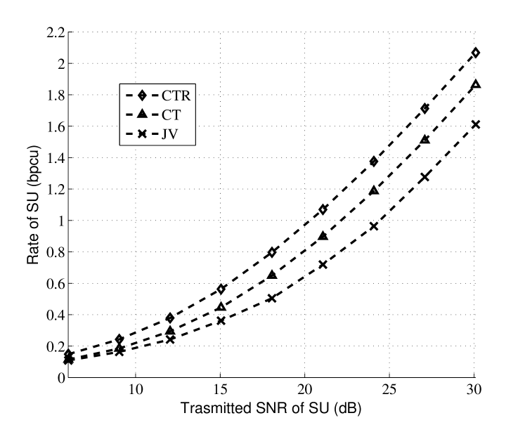
Figure 3: Comparison of the rate performance of the SU with full CSIT, under the coexistence constraint, and channels with large $|h_{34}|$ as specified in Table I. The rate is measured in bit per channel use (bpcu).

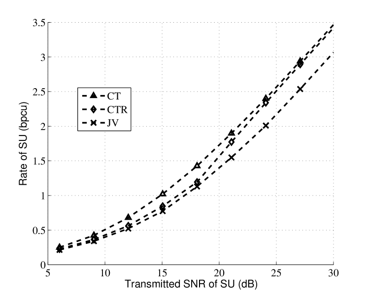
Figure 4: Comparison of the rate performance of the SU with full CSIT, under the coexistence constraint, and channels with the $|h_{34}|$ smaller than the $|h_{24}|$ as specified in Table I.

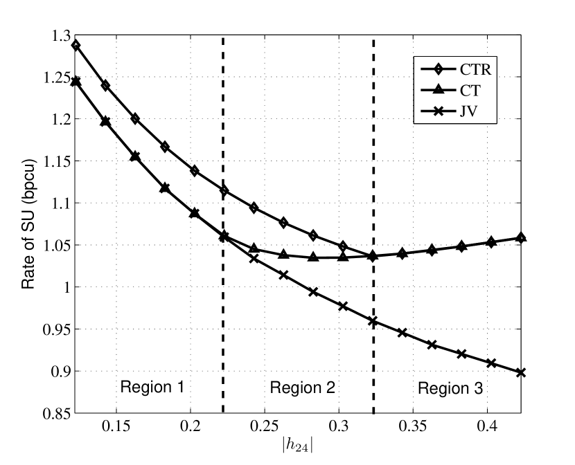
Figure 5: Comparison of the rate performance of the SU with full CSIT for different $|h_{24}|$, with 20 dB transmitted SNR and channel gains specified in Table I. Region 1 is the one where $|h_{24}|<|h_{14}|$, Region 2 is the one where $|h_{14}|<|h_{24}|<|h_{34}|$, and Region 3 is the one where $|h_{34}|<|h_{24}|$, respectively.

We first show the rate comparisons for channels with full CSIT. The channel gain of each figure is listed in Table I where the unit of the phase is radian. The $t_{1}$ in both CT and JV are $R_{T}/C(|h_{12}|^{2}P_{1}).$ In Fig. 3, we can see that with large enough $|h_{34}|$ as specified in Table I, the clean relaying from Node 3 makes the CTR have the best rate performance. Next we consider the case where $|h_{34}|$ is weaker in Fig. 4. When $|h_{34}|$ is smaller than $|h_{24}|$, the CTR may prefer clean relaying from Node 2 rather than from Node 3, that is, $P^{(3)}_{2}>P_{3}=0$. It is easy to check that in this case, the optimal $\alpha_{1}$ for the CTR is also feasible for the CT. Then comparing (2) and (7), we know that the CT performs better than the CTR as in Fig. 4. Moreover, in Fig. 3 and 4, the clean relaying of the CTR and CT yields significant gains over the JV, respectively. Next, we show how the SU’s rate changes with $|h_{24}|$ in Fig. 5. We can find out that there are three regions. In Region 1, where $|h_{24}|<|h_{14}|$, we find that the CT and JV coincide. This is consistent with [3], where JV is proved to be optimal in this region when relaying from Node 3 is prohibited. In Region 2 and 3, $|h_{24}|>|h_{14}|$, the JV wastes lots of power on the relaying since the SU produces large interference at Node 4. The CT performs better than the JV due to the clean relaying. In Region 2, $|h_{24}|<|h_{34}|$, the CTR performs better than the CT since the CTR can use a better relaying path than that of CT in Phase 3. In Region 3, $|h_{24}|>|h_{34}|$, the CT performs the best according to previously discussions for Fig. 4. However, the CT and CTR have the same performance due to the following reasons. In the channel setting for Fig. 5 listed in Table I, we find that the first term of the $\min\{.\}$ in (2) is selected, which is the same as (7). Moreover, since this term is independent of $\theta_{1}$, the relaying phase $\theta_{1}$ for the CTR is chosen as $\theta_{14}-\theta_{24}$ from (2). Together with the power allocation as in the discussions for Fig. 4, the constraints for coexistence (2) and (8) are the same in this simulation. The optimal $\alpha_{1}$ of CTR and CT are also the same, and the CTR and CT have the same rate performance.

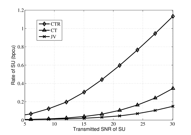
Figure 6: Comparison of the rate performance of the SU under the coexistence constraint, and fast Rayleigh fading channels with the statics of CSIT. The channel variances are listed in Table II.

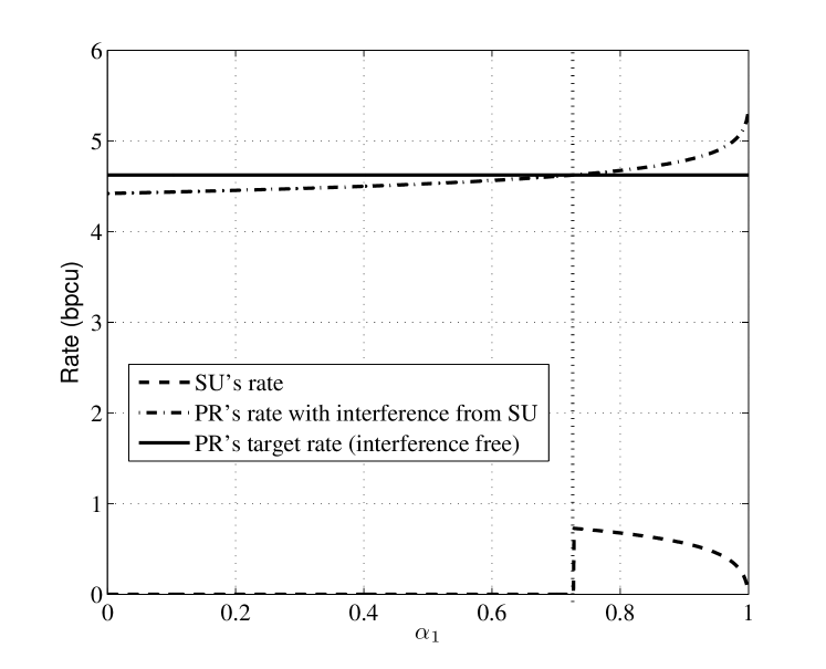
Figure 7: Rate performance of the SU of CTR versus the common message relaying ratio $\alpha_{1}$, under fast Rayleigh fading channels with the statics of CSIT. The transmit SNR of SU is 20 dB and the channel variances are listed in Table II.

Next we consider the rate performance in the fast Rayleigh faded channels with the statistics of CSIT. The channel variance of each link is listed in Table II. As shown in Fig. 6, the CTR outperforms the CT and JV, which is consistent with the discussions under Proposition 1 in Section V. The $t_{1}$ in the JV is set to $R_{T}/{\mathbf{E}}[C(|h_{12}|^{2}P_{1})]$. When the SU’s transmitted SNR is low, the CT (also JV) can only support very low rate as shown in Fig. 6. This is because that the PU’s transmitted SNR is set to 20 dB, then the interference at Node 3 is relatively large for the SU when the SU’s transmitted SNR is small. According to Proposition 1, the SU of CT (also JV) can only treat interference from the PU as noise, which degrades the rate performance a lot. However, the MAC decoder of CTR at Node 3 can avoid this problem. In Fig. 7 we show an example to verify the results in Corollary 2. We can find that the optimal $\alpha_{1}$ which maximizes the SU’s rate also make the equality in the constraint for coexistence (3) valid. That is, the optimal $\alpha_{1}$ is the minimum $\alpha_{1}$ which makes the PU’s rate with the interference from SU the same as the interference-free rate.

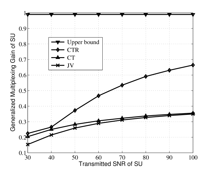
Figure 8: Comparison of the generalized multiplexing gain performance of the SU with full CSIT, under channels with large $|h_{34}|$ as specified in Table I. The upper bound is computed by (24) with $m=0.99$.

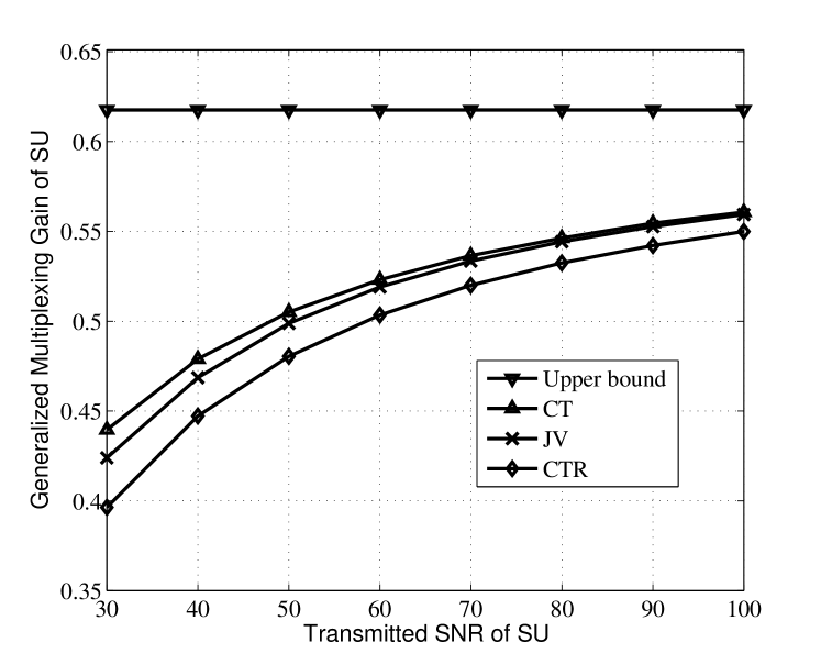
Figure 9: Comparison of the generalized multiplexing gain performance of the SU with full CSIT, under channels with small $|h_{34}|$ as specified in Table I. The upper bound is computed by (24) with $m=0.99$.

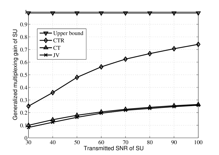
Figure 10: Comparison of the generalized multiplexing gain performance of the SU, under fast Rayleigh fading channels with the statistics of CSIT. The channel variances are listed in Table II. The upper bound is computed by (36) with $m=0.99$.

Finally, we show the multiplexing gain comparisons in the following. Following the spirit of [21], we use the generalized multiplexing gain (GMG) of the SU, which is defined as $R_{2}/\log\bar{P}_{c}$, as the performance metric for finite SNR. As $\bar{P}_{c}$ approaches infinity, the GMG will approach the multiplexing gain defined in (11). We first show the full CSIT cases in Fig. 8 and 9 with channels specified in Table I respectively. In our simulation, we set a lower bound for $t_{3}$ as 0.01 when $t_{3}\neq 0$, and $m$ in Corollary 1 will be upper-bounded by 1-0.01=0.99. We then use the multiplexing gain in (24) with $m=0.99$ as the GMG upper bound in Fig. 8 and 9. With large $|h_{34}|$ as in Table I, the GMG advantages of the CTR over the JV can be seen from Fig. 8. When the transmitted SNR is larger than 40 dB, we can find that the curve of CTR diverges from those of the CT and JV. This is because the CTR selects pure receiver relaying in this SNR region. Since $|h_{14}|<|h_{13}|$ in this simulation, according to discussions under Corollary 1, the CTR with pure receiver relaying has larger GMG than those of the CT and JV when $t_{3}$ is small and the SNR is large enough. Also when the SNR increases, the GMG of the CTR will approach the upper bound (24). Note that we plot the figures according to the transmitted SNR not the common received SNR in most of the literatures. The transmitted SNR is much larger than the received SNR since the $|h_{23}|$ of Fig. 8 in Table I is small. It then takes larger transmit SNR than the common received SNR for the GMG to approach the upper bound (multiplexing gain). In Fig. 9, we show the case with small $|h_{34}|$. The CT performs the best while the CTR performances the worst. However, as predicted by Corollary 1, even though the CTR has the worst GMG, it will approach the GMGs of CT and JV as the SNR increases. The GMG results for the fading channels with the statistics of CSIT are shown in Fig. 10. The GMG upper bound is computed from Corollary 3 with $m=0.99$ as in Fig. 8. According to the discussions for Fig. 6, the CT and JV always have worse GMG than that of the CTR according to Proposition 1.

VII Conclusion

In this paper, we considered the interference-mitigation based cognitive radio where the SU must meet the coexistence constraint to maintain the rate performance of the PU. We proposed two new transmission schemes aided by the clean relaying named as the clean transmitter relaying and the clean transmitter-receiver relaying aided cognitive radio, respectively. Compared with the previous DPC-based cognitive radio without clean relaying, the proposed schemes provide significant rate gains in a variety of channels with different levels of CSIT. Moreover, the implementation complexity of the CTR is much lower than that of the DPC-based cognitive radio.

-A Proof of Theorem 1

Let $X_{1}$ be zero mean Gaussian with variance $P_{1}$, the PU then generates its random codebook according to the distribution of $X_{1}$ with rate $R_{T}$. From [22] we know that the fractional decoding interval must satisfy $t_{1}>R_{T}/I(X_{1};Y_{2})$ to ensure the successful decoding of $w_{1}$ using the received symbols from Node 2 in Phase 1. It then results in the constraint (9) from (1).

We now invoke Lemma 1 to derive the coexistence constraint. From (3) in Phase 2, (4) in Phase 3 and the channel model (1), we know that within the $n$-symbol time, $K_{X_{1}^{n}}=P_{1}\mathbf{I}_{n}$, the equivalent channel at Node 4

$${\mathbf{H}}^{n}=\mathrm{diag}\Bigg{(} h_{14}\mathbf{I}_{\lfloor t_{1}n\rfloor},\;\left(|h_{14}|+|h_{24}|\sqrt{\alpha_{1}\frac{P_{2}}{P_{1}}}\right)e^{j\theta_{14}}\mathbf{I}_{\lfloor t_{2}n\rfloor},\left(|h_{14}|+|h_{24}|\sqrt{P_{2}/P_{1}}\right){\rm e}^{j\theta_{14}}\mathbf{I}_{\lfloor t_{3}n\rfloor}\Bigg{)}$$

and the equivalent noise has covariance matrix $K_{Z^{n}}=\mathrm{diag}\left(\mathbf{I}_{\lfloor t_{1}n\rfloor},(1+|h_{24}|^{2}(1-\alpha_{1})P_{2})\mathbf{I}_{\lfloor t_{2}n\rfloor},{\mathbf{I}}_{\lfloor t_{3}n\rfloor}\right),$ since the DPC encoded $X^{D}_{2}$ is Gaussian with variance $(1-\alpha_{1})P_{2}$ and independent of $X_{1}$ [4]. Then by invoking Lemma 1, we have (8) to ensure that $R_{T}$ is single-user achievable. Finally, since Node 2 uses $h_{13}X_{1}$ as the noncausal side-information at the transmitter in Phase 2, by applying the well-known DPC result [4] we have (7).

-B Proof of Corollary 1

We will consider two cases, that is, pure receiver and pure transmitter relaying. These two schemes can achieve multiplexing gains $m$ and $(1-C(|h_{14}|^{2}\stackrel{{\scriptstyle\;}}{{\bar{P}_{1}}})/C(|h_{12}|^{2}\stackrel{{\scriptstyle\;}}{{\bar{P}_{1}}}))^{+}$, respectively. When the channels conditions $|h_{13}|>|h_{14}|$ and $|h_{12}|>|h_{14}|$ are both valid, both schemes are feasible and the CTR can achievable the best multiplexing gain of these two schemes as (24). If only one of the channel conditions is valid, the multiplexing gain of the corresponding feasible scheme will be chosen by (24).

We first show that if $|h_{13}|>|h_{14}|$, as (25), the multiplexing gain $1-t_{3}$ is achievable by the pure receiver relaying. In this scheme, $t_{1}=\alpha_{1}=0$, $P_{2}^{(3)}=0$, and $t_{3}=1-t_{2}$, then we may set $P_{3}=P_{2}=\bar{P}_{c}$ from (23). Without loss of generality, we can set $R_{T}=C(|h_{14}|^{2}\stackrel{{\scriptstyle\;}}{{\bar{P}_{1}}})$ in the following analysis since $R_{T}\leq C(|h_{14}|^{2}\stackrel{{\scriptstyle\;}}{{\bar{P}_{1}}})$ from the channel capacity theorem [13]. With the above parameter selections, the constraint for coexistence (2), and the constraint $t_{2}C(|h_{23}\sqrt{\alpha_{1}P_{2}/P_{1}}{\rm e}^{j\theta_{1}}+h_{13}|^{2}P_{1})\geq R_{T}^{\prime}$ to validate $u_{Rx}=1$ respectively reduce to

$$C(|h_{14}|^{2}\stackrel{{\scriptstyle\;}}{{\bar{P}_{1}}})<t_{2}\cdot C\!\left(\!\frac{|h_{14}|^{2}\bar{P}_{1}}{1+|h_{24}|^{2}\stackrel{{\scriptstyle\;}}{{\bar{P}_{c}}}}\!\right)+(1-t_{2})C\left(\!\left(|h_{14}|\sqrt{\stackrel{{\scriptstyle\;}}{{\bar{P}_{1}}}}+|h_{34}|\sqrt{\stackrel{{\scriptstyle\;}}{{\bar{P}_{c}}}}\right)^{\!2}\!\right)\!,\mbox{and}\;\;t_{2}\geq\frac{C(|h_{14}|^{2}\stackrel{{\scriptstyle\;}}{{\bar{P}_{1}}})}{C(|h_{13}|^{2}\stackrel{{\scriptstyle\;}}{{\bar{P}_{1}}})}.$$ (37)

When $\bar{P}_{c}\rightarrow\infty$, we can find that the range of $t_{2}$ to validate (37) is $\frac{C(|h_{14}|^{2}\stackrel{{\scriptstyle\;}}{{\bar{P}_{1}}})}{C(|h_{13}|^{2}\stackrel{{\scriptstyle\;}}{{\bar{P}_{1}}})}\leq t_{2}<1.$ Therefore we need $t_{3}\in(0,\,1-C(|h_{14}|^{2}\bar{P}_{1})/C(|h_{13}|^{2}\bar{P}_{1})]$ to meet the constraints. From (2), (11) and the fact that $R^{m}_{T}=R^{\prime}_{T}$ since $u_{Rx}=1$, it is easy to see that the multiplexing gain $t_{2}=1-t_{3}$ is achievable, and (25) is valid. Note that our selection of $t_{2}$ and $\alpha_{1}$ is definitely a suboptimal choice with respect to (2). If $|h_{13}|\leq|h_{14}|$ and $t_{1}=0$, there will be no relaying in this case since Node 3 can not decode $w_{1}$ before the end of Phase 2. Then the multiplexing gain is zero for pure receiver relaying as in (25).

Now we show that when $|h_{14}|<|h_{12}|$, the multiplexing gain $1-C(|h_{14}|^{2}\stackrel{{\scriptstyle\;}}{{\bar{P}_{1}}})/C(|h_{12}|^{2}\stackrel{{\scriptstyle\;}}{{\bar{P}_{1}}})$ in (24) is achievable with only transmitter relaying ($t_{3}=0$). To prove this, we sub-optimally set $t_{1}=\frac{C(|h_{14}|^{2}\stackrel{{\scriptstyle\;}}{{\bar{P}_{1}}})}{C(|h_{12}|^{2}\stackrel{{\scriptstyle\;}}{{\bar{P}_{1}}})}$, $t_{2}=1-t_{1}$ and $\theta_{1}=\theta_{14}-\theta_{24}$. Together with the setting $R_{T}=C(|h_{14}|^{2}\stackrel{{\scriptstyle\;}}{{\bar{P}_{1}}})$ as describe previously, the coexistence constraint in (2) then becomes

$$C(|h_{14}|^{2}{P}_{1})<C\Bigg{(}\frac{\big{(}|h_{14}|+|h_{24}|\sqrt{\alpha_{1}P_{2}/{P}_{1}}\big{)}^{2}{P}_{1}}{1+|h_{24}|^{2}(1-\alpha_{1})P_{2}}\Bigg{)}.$$ (38)

With $t_{2}P_{2}=\bar{P}_{c}$ from (23) and $P_{1}=\stackrel{{\scriptstyle\;}}{{\bar{P}_{1}}}$ from (15), as $\bar{P}_{c}\rightarrow\infty$, (38) becomes $|h_{14}|^{2}\stackrel{{\scriptstyle\;}}{{\bar{P}_{1}}}<\frac{\alpha_{1}}{1-\alpha_{1}}.$ Then we have $\alpha_{1}>|h_{14}|^{2}\stackrel{{\scriptstyle\;}}{{\bar{P}_{1}}}/(1+|h_{14}|^{2}\stackrel{{\scriptstyle\;}}{{\bar{P}_{1}}})$ to meet the constraint for coexistence. It can be easily seen that with the selected $\alpha_{1}$, $\theta_{1}$, and $t_{2}$, when $\bar{P}_{c}\rightarrow\infty$, $R^{m}_{T}=R^{\prime}_{T}$ in (2). Therefore, from (2) and (11) we can find that the multiplexing gain $t_{2}=1-C(|h_{14}|^{2}\stackrel{{\scriptstyle\;}}{{\bar{P}_{1}}})/C(|h_{12}|^{2}\stackrel{{\scriptstyle\;}}{{\bar{P}_{1}}})$ is achievable. Finally, when $|h_{14}|\geq|h_{12}|$ the function $(.)^{+}$ in (24) will force the multiplexing gain to be zero. In this case, the coexistence constraint is violated since Node 2 cannot relay without correct knowledge of $w_{1}$.

-C Proof of Proposition 1

From [5], by treating $X_{1}$ as non-causally known transmitter side-information, the following rate is achievable by the LA-GPC

$$\max_{\beta}\{{\mathbf{E}}\big{[}\log\big{(}(|H_{23}|^{2}\bar{P}_{2}+|H_{13}|^{2}\bar{P}_{1}+1)\bar{P}_{2}\big{)}\big{]}-f(\beta)\},$$ (39)

where $f(\beta)\triangleq{\mathbf{E}}\big{[}\log\big{(}\bar{P}_{1}\bar{P}_{2}|H_{13}-\beta H_{23}|^{2}+\bar{P}_{2}+|\beta|^{2}\bar{P}_{1}\big{)}\big{]},$ and $\beta\in\mathds{C}$ is the precoding coefficient of the LA-GPC. Note that solving (39) over $\beta$ is the same as minimizing $f(\beta)$. In the following we will show that $f(0)$ is the minimal. We know that for any $\beta$

$$f(0)={\mathbf{E}}\big{[}\log\big{(}\bar{P}_{1}\bar{P}_{2}|H_{13}|^{2}+\bar{P}_{2}\big{)}\big{]} \leq{\mathbf{E}}\big{[}\log\big{(}\bar{P}_{1}\bar{P}_{2}(1+|\beta|^{2}\sigma^{2}_{23}/\sigma^{2}_{13})|H_{13}|^{2}+\bar{P}_{2}\big{)}\big{]}$$

$$={\mathbf{E}}\big{[}\log\big{(}\bar{P}_{1}\bar{P}_{2}|H_{13}-\beta H_{23}|^{2}+\bar{P}_{2}\big{)}\big{]},$$ (40)

where the last equality comes from the fact that since $H_{23}$ and $H_{13}$ are independent zero-mean Gaussian distributed with variance $\sigma^{2}_{23}$ and $\sigma^{2}_{13}$, respectively, $H_{13}-\beta H_{23}$ is also zero-mean Gaussian distributed with variance $\sigma^{2}_{13}+|\beta|^{2}\sigma^{2}_{23}$. Thus $(1+|\beta|^{2}\sigma^{2}_{23}/\sigma^{2}_{13})|H_{13}|^{2}$ and $|H_{13}-\beta H_{23}|^{2}$ have the same distribution. Moreover, for any $\beta$,

$${\mathbf{E}}\big{[}\log\big{(}\bar{P}_{1}\bar{P}_{2}|H_{13}-\beta H_{23}|^{2}+\bar{P}_{2}\big{)}\big{]}\leq{\mathbf{E}}\big{[}\log\big{(}\bar{P}_{1}\bar{P}_{2}|H_{13}-\beta H_{23}|^{2}+\bar{P}_{2}+|\beta|^{2}\bar{P}_{1}\big{)}\big{]}=f(\beta).$$

Combining the above equation with (40), we know that $\beta=0$ minimizes $f(\beta)$ and thus maximizes (39). Substituting $\beta=0$ into (39) we get (26).

-D Proof of Theorem 3

To meet the coexistence constraint, we invoke Lemma 1 again. Following the steps for proving (2) in Theorem 2, from (27), (28), (1), and Lemma 1, to ensure that the target PU’s rate is single-user achievable

$$R_{T}\leq \frac{1}{n}\sum_{t=1}^{\lfloor t_{1}n\rfloor}\log\left(1+|h_{14}(t)|^{2}P_{1}\right)+\frac{1}{n}\sum_{t=\lfloor t_{1}n\rfloor+1}^{\lfloor t_{1}n\rfloor+\lfloor t_{2}n\rfloor}\log\left(1+\frac{\Big{|}h_{14}(t)+\sqrt{\frac{\alpha_{1}P_{2}}{P_{1}}}h_{24}(t)\Big{|}^{2}P_{1}}{1+|h_{24}(t)|^{2}(1-\alpha_{1})P_{2})}\right)$$

$$+\frac{1}{n}\sum_{t=n-\lfloor t_{3}n\rfloor+1}^{n}\log\left(1+\Bigg{|}h_{14}(t)+\sqrt{\frac{P^{(3)}_{2}}{P_{1}}}h_{24}(t)+\sqrt{\frac{P_{3}}{P_{1}}}h_{34}(t)\Bigg{|}^{2}P_{1}\right),$$ (41)

where $h_{ij}(t)$ is the realization of the random channel $H_{ij}$ at time $t$. When $n$ is large enough, the first term of the RHS of (41) can be rewritten as

$$\frac{1}{n}\sum_{t=1}^{\lfloor t_{1}n\rfloor}\log\left(1+|h_{14}(t)|^{2}P_{1}\right)=t_{1}\frac{1}{\lfloor t_{1}n\rfloor}\sum_{t=1}^{\lfloor t_{1}n\rfloor}\log\left(1+|h_{14}(t)|^{2}P_{1}\right)=t_{1}{\mathbf{E}}[\log(1+|H_{14}|^{2}P_{1})],$$ (42)

where the last equality comes from the assumption that the channel coefficients are i.i.d. and applying the ergodicity property. After applying the same steps to the rest two terms of the RHS of (41), we have the constraint for coexistence (3).

The achievable rate of the SU in (29) can be obtained similarly. As for the steps to obtain (41), we still invoke Lemma 2 but modify the proof steps of Theorem 2 with the channel coefficients replaced by $h_{ij}(t)$. Then we invoke the channel ergodicity as the proof steps in (42) to reach (29). The details are omitted.

TABLE I: Channel gains in (1) Used in the Simulations (Full CSIT)

Figure	$h_{14}$	$h_{24}$	$h_{34}$	$h_{13}$	$h_{23}$	$h_{12}$
3	$0.36e^{1.6j}$	$0.45e^{1.6j}$	$0.96e^{-3.1j}$	$0.96e^{-0.69j}$	$0.24e^{-1.89j}$	$e^{-2.28j}$
4	$0.22e^{-1.6j}$	$0.92e^{0.45j}$	$0.74e^{1.19j}$	$0.25e^{-0.69j}$	$0.32e^{-1.89j}$	$e^{1.4j}$
5	$0.22e^{-0.26j}$	varying $|h_{24}|$, $\theta_{24}=\frac{\pi}{4}$	$0.32e^{-2.16j}$	$0.52e^{-0.95j}$	$0.19e^{0.22j}$	$e^{0.96j}$
8	$0.36e^{-0.78j}$	$0.95e^{1.95j}$	$2.86e^{2.09j}$	$0.96e^{0.87j}$	$0.24e^{1.84j}$	$e^{-0.965j}$
9	$0.22e^{-1.6j}$	$0.92e^{0.45j}$	$0.74e^{1.19j}$	$0.15e^{-0.69j}$	$0.62e^{-1.89j}$	$e^{1.4j}$

TABLE II: Channel Variances of Rayleigh Fading Channels in (1)
Used in the Simulations (Statistics of CSIT)

Figure	$\sigma^{2}_{14}$	$\sigma^{2}_{24}$	$\sigma^{2}_{34}$	$\sigma^{2}_{13}$	$\sigma^{2}_{23}$	$\sigma^{2}_{12}$
6	0.4	0.21	0.91	0.82	0.88	1
7	0.4	0.89	0.2	0.95	0.88	1
10	0.22	0.12	0.87	0.92	0.96	1

References

- [1] J. Mitola, “Cognitive radio: An integrated agent architecture for software defined radio,” Ph.D. dissertation, KTH Royal Inst. Technology, Stockholm, Sweden, 2000.
- [2] N. Devroye, P. Mitran, and V. Tarokh, “Achievable rates in cognitive radio channels,” IEEE Trans. Inform. Theory, vol. 52, no. 5, pp. 1813–1827, May 2006.
- [3] A. Jovicic and P. Viswanath, “Cognitive radio: An information-theoretic perspective,” IEEE Trans. Inform. Theory, vol. 55, no. 9, pp. 3945–3958, Sept. 2009.
- [4] M. H. M. Costa, “Writing on dirty paper,” IEEE Trans. Inform. Theory, vol. 29, pp. 439–441, May 1983.
- [5] P.-H. Lin, S.-C. Lin, C.-P. Lee, and H.-J. Su, “Cognitive radio with partial channel state information at the transmitter,” IEEE Trans. Wireless Commun., vol. 9, no. 11, pp. 3402–3413, Nov. 2010.
- [6] N. Liu and S. Ulukus, “Capacity region and optimum power control strategies for fading gaussian multiple access channels with common data,” IEEE Trans. Commun., vol. 54, no. 10, pp. 1815–1826, 2006.
- [7] T. M. Cover and S. Pombra, “Gaussian feedback capacity,” IEEE Trans. Inform. Theory, vol. 35, no. 1, pp. 37–43, Jan. 1989.
- [8] U. Erez and S. ten Brink, “A close to capacity dirty paper coding scheme,” IEEE Trans. Inform. Theory, vol. 51, no. 10, pp. 3417–3432, Oct. 2005.
- [9] I.-H. Wang and D. Tse, “Interference mitigation through limited receiver cooperation,” submitted to IEEE Transcation on Information theory, 2009.
- [10] C. Ng, N. Jindal, A. Goldsmith, and U. Mitra, “Capacity gain from two-transmitter and two-receiver cooperation,” IEEE Trans. Inform. Theory, vol. 53, no. 10, pp. 3822–3827, 2007.
- [11] P.-H. Lin, S.-C. Lin, H.-J. Su, and Y.-W. P. Hong, “Cognitive radio with unidirectionaltransmitter and receiver cooperations,” in Conference on Information Sciences and Systems (CISS), Mar. 2010.
- [12] E. Viterbo and J. Boutros, “A universal lattice code decoder for fading channels,” IEEE Trans. Inform. Theory, vol. 45, no. 5, pp. 1639–1642, July 1999.
- [13] T. Cover and J. Thomas, Elements of Information Theory. New York: Wiley, 1991.
- [14] L. Zheng and D. N. C. Tse, “Diversity and multiplexing: A fundamental tradeoff in multiple-antenna channels,” IEEE Transactions on Information Theory, vol. 49, no. 5, pp. 1073– 1096, May 2003.
- [15] J. Tugnait, L. Tong, and Z. Ding, “Single-user channel estimation and equalization,” IEEE Signal Processing Mag., vol. 17, no. 3, pp. 16–28, May 2000.
- [16] R. Otnes and M. Tuchler, “Iterative channel estimation for turbo equalization of time-varying frequency-selective channels,” IEEE Trans. Wireless Commun., vol. 3, no. 6, pp. 1918–1923, Nov. 2004.
- [17] D. Slepian and J. Wolf, “A coding theorem for multiple access channels with correlated sources,” Bell Syst. Tech. J, vol. 52, no. 7, pp. 1037–1076, Sep. 1973.
- [18] S. Pombra and T. Cover, “Non white Gaussian multiple access channels with feedback,” IEEE Trans. Inform. Theory, vol. 40, no. 3, pp. 885–892, May 1994.
- [19] S. I. Gel’fand and M. S. Pinsker, “Coding for channels with random parameters,” Probl. Contr. and Inform. Theory, vol. 9, no. 1, pp. 19–31, 1980.
- [20] S. Boyd and L. Vandenberghe, Convex Optimization. Cambridge University Press, 2004.
- [21] E. Stauffer, O. Oyman, R. Narasimhan, and A. Paulraj, “Finite-SNR diversity-multiplexing tradeoffs in fading relay channels,” IEEE J. Select. Areas Commun., vol. 25, no. 2, pp. 245–257, Feb. 2007.
- [22] K. Azarian, H. El-Gamal, and P. Schniter, “On the achievable diversity-multiplexing tradeoff in half-duplex cooperative channels,” IEEE Trans. Inform. Theory, vol. 51, no. 12, pp. 4152–4172, Dec. 2005.