Relativistic coupled-cluster calculations of nuclear spin-dependent parity non-conservation in Cs, Ba⁺ and Ra⁺

Abstract

We have developed a relativistic coupled-cluster theory to incorporate nuclear spin-dependent interaction Hamiltonians perturbatively. This theory is ideal to calculate parity violating nuclear spin-dependent electric dipole transition amplitudes, $E1_{\rm PNC}^{\rm NSD}$, of heavy atoms. Experimental observation of which is a clear signature of nuclear anapole moment, the dominant source of nuclear spin-dependent parity violation in atoms and ions. We apply the theory to calculate $E1_{\rm PNC}^{\rm NSD}$ of Cs, which to date has provided the best atomic parity violation measurements. We also calculate $E1_{\rm PNC}^{\rm NSD}$ of Ba⁺ and Ra⁺, candidates of ongoing and proposed experiments.

The effects of parity nonconservation (PNC) in atoms occur in two forms, nuclear spin-independent (NSI) and nuclear spin-dependent (NSD). The former is well studied and experimentally observed in several atoms. The signature of the later (NSD) has been observed only in one experiment with Cs wood-97 and the same experiment has provided the most accurate results on NSI atomic PNC as well. In an atom or ion the most dominant source of NSD-PNC is the nuclear anapole moment (NAM), a parity odd nuclear electromagnetic moment. It was first suggested by Zeldovich zeldovich-58 and arises from parity violating phenomena within the nucleus.

One major hurdle to a clear and unambiguous observation of NAM is the large NSI signal, which overwhelms the NSD signal. However, proposed experiments with single Ba⁺ ion fortson-93 could probe PNC in the $s_{1/2}-d_{5/2}$ transition, where the NSI component is zero. This could then provide an unambiguous observation of NSD-PNC and NAM in particular. The ongoing experiments with atomic Ytterbium tsigutkin-09 is another possibility, the $6s^{2}\;{}^{1}S_{0}-6s5d\;^{3}D_{2}$ transition, to observe NSD-PNC with minimal mixture from the NSI component. One crucial input, which is also the source of large uncertainty, to extract the value of NAM is the input from atomic theory calculations. Considering this, it is important to employ reliable and accurate many-body theory in the atomic theory calculations.

The coupled-cluster (CC) theorycoester-58 ; coester-60 is one of the most reliable many-body theory to incorporate electron correlation in atomic calculations. It has been used with great success in nuclear hagen-08 , atomic eliav-94 ; nataraj-08 ; pal-07 , molecular isaev-04 and condensed matter bishop-09 physics. In atomic physics, the relativistic coupled-cluster (RCC) theory has been used extensively in atomic properties calculations, for example, hyperfine structure constants pal-07 ; sahoo-09 and electromagnetic transition properties thierfelder-09 ; sahoo-09a . In atomic PNC calculations too, RCC is the preferred theory and several groups have used it to calculate NSI-PNC of atoms wansbeek-08 ; pal-09 ; porsev-10 . However, the calculations in Ref. wansbeek-08 are entirely based on RCC with a variation we refer to as perturbed RCC (PRCC), where as the calculations in Ref. pal-09 ; porsev-10 are based on sum over states with CC wave functions.

To date, the use of PRCC in atomic PNC is limited to NSI-PNC. In this letter we report the PRCC theory to calculate NSD-PNC in atoms. Such a development is timely as the recent experimental proposals on Ba⁺ and Ra⁺ sahoo-11 and observation of large enhancement in atomic Yb tsigutkin-09 shall require precision atomic theory to examine the systematics and interpret the results. It must perhaps be mentioned that, in an earlier work we had developed and calculated electric dipole moment of atomic Hg latha-09 using PRCC theory.

RCC theory.—In the RCC method, the atomic state is expressed in terms of $T$ and $S$, the closed-shell and one-valence cluster operators respectively, as

$$|\Psi_{v}\rangle=e^{T^{(0)}}\left[1+S^{(0)}\right]|\Phi_{v}\rangle,$$ (1)

where $|\Phi_{v}\rangle$ is the one-valence Dirac-Fock reference state. It is obtained by adding an electron to the closed-shell reference state, $|\Phi_{v}\rangle=a^{\dagger}_{v}|\Phi_{0}\rangle$. In the coupled-cluster singles doubles (CCSD) approximation $T^{(0)}=T^{(0)}_{1}+T^{(0)}_{2}$ and $S^{(0)}=S^{(0)}_{1}+S^{(0)}_{2}$. The open-shell cluster operators are solutions of the nonlinear equations mani-10

$$\langle\Phi_{v}^{p}|\bar{H}_{N}\!+\!\{\mathchoice{\vbox{\hbox to0.0pt{\kern 5.00002pt\kern 4.56248pt\hbox{\vrule width=0.50003pt,height=0.0pt,depth=2.15277pt\vrule width=13.02663pt,height=0.0pt,depth=0.50003pt\vrule width=0.50003pt,height=0.0pt,depth=2.15277pt}\hss}\vskip 2.15277pt\vskip 6.83331pt}}{\vbox{\hbox to0.0pt{\kern 5.00002pt\kern 4.56248pt\hbox{\vrule width=0.50003pt,height=0.0pt,depth=2.15277pt\vrule width=13.02663pt,height=0.0pt,depth=0.50003pt\vrule width=0.50003pt,height=0.0pt,depth=2.15277pt}\hss}\vskip 2.15277pt\vskip 6.83331pt}}{\vbox{\hbox to0.0pt{\kern 5.00002pt\kern 3.19374pt\hbox{\vrule width=0.50003pt,height=0.0pt,depth=2.15277pt\vrule width=9.19162pt,height=0.0pt,depth=0.50003pt\vrule width=0.50003pt,height=0.0pt,depth=2.15277pt}\hss}\vskip 2.15277pt\vskip 4.78333pt}}{\vbox{\hbox to0.0pt{\kern 5.00002pt\kern 2.28123pt\hbox{\vrule width=0.50003pt,height=0.0pt,depth=2.15277pt\vrule width=7.60829pt,height=0.0pt,depth=0.50003pt\vrule width=0.50003pt,height=0.0pt,depth=2.15277pt}\hss}\vskip 2.15277pt\vskip 3.41666pt}}\bar{H}_{N}S^{(0)}\}|\Phi_{v}\rangle = E_{v}^{\rm att}\langle\Phi_{v}^{p}|S^{(0)}_{1}|\Phi_{v}\rangle,$$ (2a)

$$\langle\Phi_{va}^{pq}|\bar{H}_{N}+\{\mathchoice{\vbox{\hbox to0.0pt{\kern 5.00002pt\kern 4.56248pt\hbox{\vrule width=0.50003pt,height=0.0pt,depth=2.15277pt\vrule width=13.02663pt,height=0.0pt,depth=0.50003pt\vrule width=0.50003pt,height=0.0pt,depth=2.15277pt}\hss}\vskip 2.15277pt\vskip 6.83331pt}}{\vbox{\hbox to0.0pt{\kern 5.00002pt\kern 4.56248pt\hbox{\vrule width=0.50003pt,height=0.0pt,depth=2.15277pt\vrule width=13.02663pt,height=0.0pt,depth=0.50003pt\vrule width=0.50003pt,height=0.0pt,depth=2.15277pt}\hss}\vskip 2.15277pt\vskip 6.83331pt}}{\vbox{\hbox to0.0pt{\kern 5.00002pt\kern 3.19374pt\hbox{\vrule width=0.50003pt,height=0.0pt,depth=2.15277pt\vrule width=9.19162pt,height=0.0pt,depth=0.50003pt\vrule width=0.50003pt,height=0.0pt,depth=2.15277pt}\hss}\vskip 2.15277pt\vskip 4.78333pt}}{\vbox{\hbox to0.0pt{\kern 5.00002pt\kern 2.28123pt\hbox{\vrule width=0.50003pt,height=0.0pt,depth=2.15277pt\vrule width=7.60829pt,height=0.0pt,depth=0.50003pt\vrule width=0.50003pt,height=0.0pt,depth=2.15277pt}\hss}\vskip 2.15277pt\vskip 3.41666pt}}\bar{H}_{N}S^{(0)}\}|\Phi_{v}\rangle = E_{v}^{\rm att}\langle\Phi_{va}^{pq}|S^{(0)}_{2}|\Phi_{v}\rangle,$$ (2b)

where $\bar{H}_{\rm N}=e^{-T^{(0)}}H_{\rm N}e^{T^{(0)}}$ is the similarity transformed Hamiltonian and the normal ordered atomic Hamiltonian $H_{\rm N}=H-\langle\Phi_{0}|H|\Phi_{0}\rangle$. And, $E_{v}^{\rm att}=E_{v}-E_{0},$ is the attachment energy of the valence electron. The $T^{(0)}$ are solutions of a similar set of equations, however, with $S^{(0)}=0$. A similar set of equations may be derived in the case of two-valence systems and use it in the wave function and properties calculations of atoms like Yb mani-11 .

Perturbed RCC theory.—The perturbed RCC method sahoo-06 ; mani-09 , unlike the standard time-independent perturbation theory, implicitly accounts for all the possible intermediate states in properties calculations. Consider the NSD-PNC interaction Hamiltonian

$$H_{\rm PNC}^{\rm NSD}=\frac{G_{\rm F}\mu^{\prime}_{W}}{\sqrt{2}}\sum_{i}\bm{\alpha}_{i}\cdot\mathbf{I}\rho_{\rm{N}}(r),$$ (3)

as the perturbation. Here, $\mu^{\prime}_{W}$ is the weak nuclear moment of the nucleus and $\rho_{\rm N}(r)$ is the nuclear density. The total atomic Hamiltonian is

$$H_{\rm A}=H^{\rm DC}+\lambda H_{\rm PNC}^{\rm NSD},$$ (4)

where $\lambda$ is the perturbation parameter. Mixed parity hyperfine states $|\widetilde{\Psi}_{v}\rangle$ are then the eigen states of $H_{\rm A}$. To calculate $|\widetilde{\Psi}_{v}\rangle$ from RCC, we define a new set of cluster operators $\mathbf{T}^{(1)}$, which unlike $T^{(0)}$ connects the reference state to opposite parity states. This is the result of incorporating one order of $H_{\rm PNC}^{\rm NSD}$ and for this reason we refer to $\mathbf{T}^{(1)}$ as the perturbed cluster operators. Although hyperfine states are natural to $H_{\rm PNC}^{\rm NSD}$, cluster operator $\mathbf{T}^{(1)}$ is defined to operate only in the electronic space and is a rank one operator. For this define ${\mathbf{H}}_{\rm elec}^{\rm NSD}=(G_{\rm F}\mu^{\prime}_{W})/(\sqrt{2})\sum_{i}\bm{\alpha}_{i}\rho_{\rm{N}}(r)$, which operates only in the electronic space, so that $H_{\rm PNC}^{\rm NSD}={\mathbf{H}}_{\rm elec}^{\rm NSD}\cdot\mathbf{I}$. The closed-shell exponential operator in PRCC is $e^{T^{(0)}+\lambda\mathbf{T}^{(1)}\cdot\mathbf{I}}$ and the atomic state is

$$|\widetilde{\Psi}_{0}\rangle=e^{T^{(0)}}\left[1+\lambda\mathbf{T}^{(1)}\cdot\mathbf{I}\right]|\Phi_{0}\rangle.$$ (5)

Similarly, the mixed parity state from one-valence PRCC theory is

$$|\widetilde{\Psi}_{v}\rangle=e^{T^{(0)}}\left[1+\lambda\mathbf{T}^{(1)}\cdot\mathbf{I}\right]\left[1+S^{(0)}+\lambda\mathbf{S}^{(1)}\cdot\mathbf{I}\right]|\Phi_{v}\rangle.$$ (6)

As $\mathbf{T}^{(1)}_{1}$ is one particle and rank one operator, in terms of c-tensors

$$\mathbf{T}^{(1)}_{1}=\sum_{ap}\tau_{a}^{p}\mathbf{C}_{1}(\hat{r}),$$ (7)

where $\mathbf{C}_{i}$ are c-tensor operators. Similarly, the tensor structure of $\mathbf{T}^{(1)}_{2}$ is

$$\mathbf{T}^{(1)}_{2}=\sum_{abpq}\sum_{l_{1},l_{2}}\tau_{ab}^{pq}(l_{1},l_{2})\{\mathbf{C}_{l_{1}}(\hat{r}_{1})\mathbf{C}_{l_{2}}(\hat{r}_{2})\}^{1},$$ (8)

where $\{\cdots\}^{1}$ indicates the two c-tensor operators couple to a rank one tensor operator. Based on the tensor structures, the perturbed cluster operators are diagrammatically represented as shown in Fig. 1. For the doubles $\mathbf{T}^{(1)}_{2}$, to indicate the multipole structure, an additional line is added to the interaction line. The cluster operators are solutions of the equations

$$\langle\Phi^{p}_{v}|\{\mathchoice{\vbox{\hbox to0.0pt{\kern 0.0pt\kern 4.56248pt\hbox{\vrule width=0.50003pt,height=0.0pt,depth=4.30554pt\vrule width=12.11664pt,height=0.0pt,depth=0.50003pt\vrule width=0.50003pt,height=0.0pt,depth=4.30554pt}\hss}\vskip 2.15277pt\vskip 6.83331pt}}{\vbox{\hbox to0.0pt{\kern 0.0pt\kern 4.56248pt\hbox{\vrule width=0.50003pt,height=0.0pt,depth=4.30554pt\vrule width=12.11664pt,height=0.0pt,depth=0.50003pt\vrule width=0.50003pt,height=0.0pt,depth=4.30554pt}\hss}\vskip 2.15277pt\vskip 6.83331pt}}{\vbox{\hbox to0.0pt{\kern 0.0pt\kern 3.19374pt\hbox{\vrule width=0.50003pt,height=0.0pt,depth=4.30554pt\vrule width=8.54164pt,height=0.0pt,depth=0.50003pt\vrule width=0.50003pt,height=0.0pt,depth=4.30554pt}\hss}\vskip 2.15277pt\vskip 4.78333pt}}{\vbox{\hbox to0.0pt{\kern 0.0pt\kern 2.28123pt\hbox{\vrule width=0.50003pt,height=0.0pt,depth=4.30554pt\vrule width=6.95831pt,height=0.0pt,depth=0.50003pt\vrule width=0.50003pt,height=0.0pt,depth=4.30554pt}\hss}\vskip 2.15277pt\vskip 3.41666pt}}\bar{H}_{\rm N}\mathbf{S}^{(1)}\}+\{\mathchoice{\vbox{\hbox to0.0pt{\kern 0.0pt\kern 4.56248pt\hbox{\vrule width=0.50003pt,height=0.0pt,depth=4.30554pt\vrule width=12.11664pt,height=0.0pt,depth=0.50003pt\vrule width=0.50003pt,height=0.0pt,depth=4.30554pt}\hss}\vskip 2.15277pt\vskip 6.83331pt}}{\vbox{\hbox to0.0pt{\kern 0.0pt\kern 4.56248pt\hbox{\vrule width=0.50003pt,height=0.0pt,depth=4.30554pt\vrule width=12.11664pt,height=0.0pt,depth=0.50003pt\vrule width=0.50003pt,height=0.0pt,depth=4.30554pt}\hss}\vskip 2.15277pt\vskip 6.83331pt}}{\vbox{\hbox to0.0pt{\kern 0.0pt\kern 3.19374pt\hbox{\vrule width=0.50003pt,height=0.0pt,depth=4.30554pt\vrule width=8.54164pt,height=0.0pt,depth=0.50003pt\vrule width=0.50003pt,height=0.0pt,depth=4.30554pt}\hss}\vskip 2.15277pt\vskip 4.78333pt}}{\vbox{\hbox to0.0pt{\kern 0.0pt\kern 2.28123pt\hbox{\vrule width=0.50003pt,height=0.0pt,depth=4.30554pt\vrule width=6.95831pt,height=0.0pt,depth=0.50003pt\vrule width=0.50003pt,height=0.0pt,depth=4.30554pt}\hss}\vskip 2.15277pt\vskip 3.41666pt}}\bar{H}_{\rm N}\mathbf{T}^{(1)}\}+\{\mathchoice{\vbox{\hbox to0.0pt{\kern 0.0pt\kern 4.56248pt\hbox{\vrule width=0.50003pt,height=0.0pt,depth=4.30554pt\vrule width=12.3788pt,height=0.0pt,depth=0.50003pt\vrule width=0.50003pt,height=0.0pt,depth=4.30554pt}\hss}\vskip 2.15277pt\vskip 6.83331pt}}{\vbox{\hbox to0.0pt{\kern 0.0pt\kern 4.56248pt\hbox{\vrule width=0.50003pt,height=0.0pt,depth=4.30554pt\vrule width=12.3788pt,height=0.0pt,depth=0.50003pt\vrule width=0.50003pt,height=0.0pt,depth=4.30554pt}\hss}\vskip 2.15277pt\vskip 6.83331pt}}{\vbox{\hbox to0.0pt{\kern 0.0pt\kern 3.19374pt\hbox{\vrule width=0.50003pt,height=0.0pt,depth=4.30554pt\vrule width=8.72516pt,height=0.0pt,depth=0.50003pt\vrule width=0.50003pt,height=0.0pt,depth=4.30554pt}\hss}\vskip 2.15277pt\vskip 4.78333pt}}{\vbox{\hbox to0.0pt{\kern 0.0pt\kern 2.28123pt\hbox{\vrule width=0.50003pt,height=0.0pt,depth=4.30554pt\vrule width=7.0894pt,height=0.0pt,depth=0.50003pt\vrule width=0.50003pt,height=0.0pt,depth=4.30554pt}\hss}\vskip 2.15277pt\vskip 3.41666pt}}\mathchoice{\vbox{\hbox to0.0pt{\kern 0.0pt\kern 4.02777pt\hbox{\vrule width=0.50003pt,height=0.0pt,depth=6.45831pt\vrule width=25.97014pt,height=0.0pt,depth=0.50003pt\vrule width=0.50003pt,height=0.0pt,depth=6.45831pt}\hss}\vskip 2.15277pt\vskip 6.83331pt}}{\vbox{\hbox to0.0pt{\kern 0.0pt\kern 4.02777pt\hbox{\vrule width=0.50003pt,height=0.0pt,depth=6.45831pt\vrule width=25.97014pt,height=0.0pt,depth=0.50003pt\vrule width=0.50003pt,height=0.0pt,depth=6.45831pt}\hss}\vskip 2.15277pt\vskip 6.83331pt}}{\vbox{\hbox to0.0pt{\kern 0.0pt\kern 2.81944pt\hbox{\vrule width=0.50003pt,height=0.0pt,depth=6.45831pt\vrule width=18.34131pt,height=0.0pt,depth=0.50003pt\vrule width=0.50003pt,height=0.0pt,depth=6.45831pt}\hss}\vskip 2.15277pt\vskip 4.78333pt}}{\vbox{\hbox to0.0pt{\kern 0.0pt\kern 2.01389pt\hbox{\vrule width=0.50003pt,height=0.0pt,depth=6.45831pt\vrule width=15.41838pt,height=0.0pt,depth=0.50003pt\vrule width=0.50003pt,height=0.0pt,depth=6.45831pt}\hss}\vskip 2.15277pt\vskip 3.41666pt}}H_{\rm N}\mathbf{T}^{(1)}S^{(0)}\}+\bar{\mathbf{H}}_{\rm elec}^{\rm NSD}$$

$$+\{\mathchoice{\vbox{\hbox to0.0pt{\kern 0.0pt\kern 4.56248pt\hbox{\vrule width=0.50003pt,height=0.0pt,depth=4.30554pt\vrule width=16.93887pt,height=0.0pt,depth=0.50003pt\vrule width=0.50003pt,height=0.0pt,depth=4.30554pt}\hss}\vskip 2.15277pt\vskip 6.83331pt}}{\vbox{\hbox to0.0pt{\kern 0.0pt\kern 4.56248pt\hbox{\vrule width=0.50003pt,height=0.0pt,depth=4.30554pt\vrule width=16.93887pt,height=0.0pt,depth=0.50003pt\vrule width=0.50003pt,height=0.0pt,depth=4.30554pt}\hss}\vskip 2.15277pt\vskip 6.83331pt}}{\vbox{\hbox to0.0pt{\kern 0.0pt\kern 3.19374pt\hbox{\vrule width=0.50003pt,height=0.0pt,depth=4.30554pt\vrule width=11.98607pt,height=0.0pt,depth=0.50003pt\vrule width=0.50003pt,height=0.0pt,depth=4.30554pt}\hss}\vskip 2.15277pt\vskip 4.78333pt}}{\vbox{\hbox to0.0pt{\kern 0.0pt\kern 2.28123pt\hbox{\vrule width=0.50003pt,height=0.0pt,depth=4.30554pt\vrule width=10.40274pt,height=0.0pt,depth=0.50003pt\vrule width=0.50003pt,height=0.0pt,depth=4.30554pt}\hss}\vskip 2.15277pt\vskip 3.41666pt}}\bar{\mathbf{H}}_{\rm elec}^{\rm NSD}{S}^{(0)}\}|\Phi_{v}\rangle=\Delta E_{v}\langle\Phi^{p}_{v}|\mathbf{S}^{(1)}_{1}|\Phi_{v}\rangle,$$ (9a)

$$\langle\Phi^{pq}_{vb}|\{\mathchoice{\vbox{\hbox to0.0pt{\kern 0.0pt\kern 4.56248pt\hbox{\vrule width=0.50003pt,height=0.0pt,depth=4.30554pt\vrule width=12.11664pt,height=0.0pt,depth=0.50003pt\vrule width=0.50003pt,height=0.0pt,depth=4.30554pt}\hss}\vskip 2.15277pt\vskip 6.83331pt}}{\vbox{\hbox to0.0pt{\kern 0.0pt\kern 4.56248pt\hbox{\vrule width=0.50003pt,height=0.0pt,depth=4.30554pt\vrule width=12.11664pt,height=0.0pt,depth=0.50003pt\vrule width=0.50003pt,height=0.0pt,depth=4.30554pt}\hss}\vskip 2.15277pt\vskip 6.83331pt}}{\vbox{\hbox to0.0pt{\kern 0.0pt\kern 3.19374pt\hbox{\vrule width=0.50003pt,height=0.0pt,depth=4.30554pt\vrule width=8.54164pt,height=0.0pt,depth=0.50003pt\vrule width=0.50003pt,height=0.0pt,depth=4.30554pt}\hss}\vskip 2.15277pt\vskip 4.78333pt}}{\vbox{\hbox to0.0pt{\kern 0.0pt\kern 2.28123pt\hbox{\vrule width=0.50003pt,height=0.0pt,depth=4.30554pt\vrule width=6.95831pt,height=0.0pt,depth=0.50003pt\vrule width=0.50003pt,height=0.0pt,depth=4.30554pt}\hss}\vskip 2.15277pt\vskip 3.41666pt}}\bar{H}_{\rm N}\mathbf{S}^{(1)}\}+\{\mathchoice{\vbox{\hbox to0.0pt{\kern 0.0pt\kern 4.56248pt\hbox{\vrule width=0.50003pt,height=0.0pt,depth=4.30554pt\vrule width=12.11664pt,height=0.0pt,depth=0.50003pt\vrule width=0.50003pt,height=0.0pt,depth=4.30554pt}\hss}\vskip 2.15277pt\vskip 6.83331pt}}{\vbox{\hbox to0.0pt{\kern 0.0pt\kern 4.56248pt\hbox{\vrule width=0.50003pt,height=0.0pt,depth=4.30554pt\vrule width=12.11664pt,height=0.0pt,depth=0.50003pt\vrule width=0.50003pt,height=0.0pt,depth=4.30554pt}\hss}\vskip 2.15277pt\vskip 6.83331pt}}{\vbox{\hbox to0.0pt{\kern 0.0pt\kern 3.19374pt\hbox{\vrule width=0.50003pt,height=0.0pt,depth=4.30554pt\vrule width=8.54164pt,height=0.0pt,depth=0.50003pt\vrule width=0.50003pt,height=0.0pt,depth=4.30554pt}\hss}\vskip 2.15277pt\vskip 4.78333pt}}{\vbox{\hbox to0.0pt{\kern 0.0pt\kern 2.28123pt\hbox{\vrule width=0.50003pt,height=0.0pt,depth=4.30554pt\vrule width=6.95831pt,height=0.0pt,depth=0.50003pt\vrule width=0.50003pt,height=0.0pt,depth=4.30554pt}\hss}\vskip 2.15277pt\vskip 3.41666pt}}\bar{H}_{\rm N}\mathbf{T}^{(1)}\}+\{\mathchoice{\vbox{\hbox to0.0pt{\kern 0.0pt\kern 4.56248pt\hbox{\vrule width=0.50003pt,height=0.0pt,depth=4.30554pt\vrule width=12.3788pt,height=0.0pt,depth=0.50003pt\vrule width=0.50003pt,height=0.0pt,depth=4.30554pt}\hss}\vskip 2.15277pt\vskip 6.83331pt}}{\vbox{\hbox to0.0pt{\kern 0.0pt\kern 4.56248pt\hbox{\vrule width=0.50003pt,height=0.0pt,depth=4.30554pt\vrule width=12.3788pt,height=0.0pt,depth=0.50003pt\vrule width=0.50003pt,height=0.0pt,depth=4.30554pt}\hss}\vskip 2.15277pt\vskip 6.83331pt}}{\vbox{\hbox to0.0pt{\kern 0.0pt\kern 3.19374pt\hbox{\vrule width=0.50003pt,height=0.0pt,depth=4.30554pt\vrule width=8.72516pt,height=0.0pt,depth=0.50003pt\vrule width=0.50003pt,height=0.0pt,depth=4.30554pt}\hss}\vskip 2.15277pt\vskip 4.78333pt}}{\vbox{\hbox to0.0pt{\kern 0.0pt\kern 2.28123pt\hbox{\vrule width=0.50003pt,height=0.0pt,depth=4.30554pt\vrule width=7.0894pt,height=0.0pt,depth=0.50003pt\vrule width=0.50003pt,height=0.0pt,depth=4.30554pt}\hss}\vskip 2.15277pt\vskip 3.41666pt}}\mathchoice{\vbox{\hbox to0.0pt{\kern 0.0pt\kern 4.02777pt\hbox{\vrule width=0.50003pt,height=0.0pt,depth=6.45831pt\vrule width=25.97014pt,height=0.0pt,depth=0.50003pt\vrule width=0.50003pt,height=0.0pt,depth=6.45831pt}\hss}\vskip 2.15277pt\vskip 6.83331pt}}{\vbox{\hbox to0.0pt{\kern 0.0pt\kern 4.02777pt\hbox{\vrule width=0.50003pt,height=0.0pt,depth=6.45831pt\vrule width=25.97014pt,height=0.0pt,depth=0.50003pt\vrule width=0.50003pt,height=0.0pt,depth=6.45831pt}\hss}\vskip 2.15277pt\vskip 6.83331pt}}{\vbox{\hbox to0.0pt{\kern 0.0pt\kern 2.81944pt\hbox{\vrule width=0.50003pt,height=0.0pt,depth=6.45831pt\vrule width=18.34131pt,height=0.0pt,depth=0.50003pt\vrule width=0.50003pt,height=0.0pt,depth=6.45831pt}\hss}\vskip 2.15277pt\vskip 4.78333pt}}{\vbox{\hbox to0.0pt{\kern 0.0pt\kern 2.01389pt\hbox{\vrule width=0.50003pt,height=0.0pt,depth=6.45831pt\vrule width=15.41838pt,height=0.0pt,depth=0.50003pt\vrule width=0.50003pt,height=0.0pt,depth=6.45831pt}\hss}\vskip 2.15277pt\vskip 3.41666pt}}H_{\rm N}\mathbf{T}^{(1)}S^{(0)}\}+\bar{\mathbf{H}}_{\rm elec}^{\rm NSD}$$

$$+\{\mathchoice{\vbox{\hbox to0.0pt{\kern 0.0pt\kern 4.56248pt\hbox{\vrule width=0.50003pt,height=0.0pt,depth=4.30554pt\vrule width=16.93887pt,height=0.0pt,depth=0.50003pt\vrule width=0.50003pt,height=0.0pt,depth=4.30554pt}\hss}\vskip 2.15277pt\vskip 6.83331pt}}{\vbox{\hbox to0.0pt{\kern 0.0pt\kern 4.56248pt\hbox{\vrule width=0.50003pt,height=0.0pt,depth=4.30554pt\vrule width=16.93887pt,height=0.0pt,depth=0.50003pt\vrule width=0.50003pt,height=0.0pt,depth=4.30554pt}\hss}\vskip 2.15277pt\vskip 6.83331pt}}{\vbox{\hbox to0.0pt{\kern 0.0pt\kern 3.19374pt\hbox{\vrule width=0.50003pt,height=0.0pt,depth=4.30554pt\vrule width=11.98607pt,height=0.0pt,depth=0.50003pt\vrule width=0.50003pt,height=0.0pt,depth=4.30554pt}\hss}\vskip 2.15277pt\vskip 4.78333pt}}{\vbox{\hbox to0.0pt{\kern 0.0pt\kern 2.28123pt\hbox{\vrule width=0.50003pt,height=0.0pt,depth=4.30554pt\vrule width=10.40274pt,height=0.0pt,depth=0.50003pt\vrule width=0.50003pt,height=0.0pt,depth=4.30554pt}\hss}\vskip 2.15277pt\vskip 3.41666pt}}\bar{\mathbf{H}}_{\rm elec}^{\rm NSD}{S}^{(0)}\}|\Phi_{v}\rangle=\Delta E_{v}\langle\Phi^{pq}_{vb}|\mathbf{S}^{(1)}_{2}|\Phi_{v}\rangle,$$ (9b)

Where we have used the relations $\langle\Phi^{p}_{v}|\mathbf{T}^{(1)}|\Phi_{v}\rangle=0$, and $\langle\Phi^{p}_{v}|\mathbf{T}^{(1)}S|\Phi_{v}\rangle=0$, as the bra state is valence excited. An approximate form of Eq. (9), but which contains all the important many-body effects, are the linearized cluster equations. This is obtained by considering $\mathchoice{\vbox{\hbox to0.0pt{\kern 0.0pt\kern 4.56248pt\hbox{\vrule width=0.50003pt,height=0.0pt,depth=4.30554pt\vrule width=12.3788pt,height=0.0pt,depth=0.50003pt\vrule width=0.50003pt,height=0.0pt,depth=4.30554pt}\hss}\vskip 2.15277pt\vskip 6.83331pt}}{\vbox{\hbox to0.0pt{\kern 0.0pt\kern 4.56248pt\hbox{\vrule width=0.50003pt,height=0.0pt,depth=4.30554pt\vrule width=12.3788pt,height=0.0pt,depth=0.50003pt\vrule width=0.50003pt,height=0.0pt,depth=4.30554pt}\hss}\vskip 2.15277pt\vskip 6.83331pt}}{\vbox{\hbox to0.0pt{\kern 0.0pt\kern 3.19374pt\hbox{\vrule width=0.50003pt,height=0.0pt,depth=4.30554pt\vrule width=8.72516pt,height=0.0pt,depth=0.50003pt\vrule width=0.50003pt,height=0.0pt,depth=4.30554pt}\hss}\vskip 2.15277pt\vskip 4.78333pt}}{\vbox{\hbox to0.0pt{\kern 0.0pt\kern 2.28123pt\hbox{\vrule width=0.50003pt,height=0.0pt,depth=4.30554pt\vrule width=7.0894pt,height=0.0pt,depth=0.50003pt\vrule width=0.50003pt,height=0.0pt,depth=4.30554pt}\hss}\vskip 2.15277pt\vskip 3.41666pt}}\bar{H}_{\rm N}\mathbf{T}^{(1)}\approx\mathchoice{\vbox{\hbox to0.0pt{\kern 0.0pt\kern 4.56248pt\hbox{\vrule width=0.50003pt,height=0.0pt,depth=4.30554pt\vrule width=12.3788pt,height=0.0pt,depth=0.50003pt\vrule width=0.50003pt,height=0.0pt,depth=4.30554pt}\hss}\vskip 2.15277pt\vskip 6.83331pt}}{\vbox{\hbox to0.0pt{\kern 0.0pt\kern 4.56248pt\hbox{\vrule width=0.50003pt,height=0.0pt,depth=4.30554pt\vrule width=12.3788pt,height=0.0pt,depth=0.50003pt\vrule width=0.50003pt,height=0.0pt,depth=4.30554pt}\hss}\vskip 2.15277pt\vskip 6.83331pt}}{\vbox{\hbox to0.0pt{\kern 0.0pt\kern 3.19374pt\hbox{\vrule width=0.50003pt,height=0.0pt,depth=4.30554pt\vrule width=8.72516pt,height=0.0pt,depth=0.50003pt\vrule width=0.50003pt,height=0.0pt,depth=4.30554pt}\hss}\vskip 2.15277pt\vskip 4.78333pt}}{\vbox{\hbox to0.0pt{\kern 0.0pt\kern 2.28123pt\hbox{\vrule width=0.50003pt,height=0.0pt,depth=4.30554pt\vrule width=7.0894pt,height=0.0pt,depth=0.50003pt\vrule width=0.50003pt,height=0.0pt,depth=4.30554pt}\hss}\vskip 2.15277pt\vskip 3.41666pt}}{H}_{\rm N}\mathbf{T}^{(1)}$, and $\bar{\mathbf{H}}_{\rm elec}^{\rm NSD}\approx\mathbf{H}_{\rm elec}^{\rm NSD}+\mathchoice{\vbox{\hbox to0.0pt{\kern 0.0pt\kern 4.56248pt\hbox{\vrule width=0.50003pt,height=0.0pt,depth=4.30554pt\vrule width=17.20103pt,height=0.0pt,depth=0.50003pt\vrule width=0.50003pt,height=0.0pt,depth=4.30554pt}\hss}\vskip 2.15277pt\vskip 6.83331pt}}{\vbox{\hbox to0.0pt{\kern 0.0pt\kern 4.56248pt\hbox{\vrule width=0.50003pt,height=0.0pt,depth=4.30554pt\vrule width=17.20103pt,height=0.0pt,depth=0.50003pt\vrule width=0.50003pt,height=0.0pt,depth=4.30554pt}\hss}\vskip 2.15277pt\vskip 6.83331pt}}{\vbox{\hbox to0.0pt{\kern 0.0pt\kern 3.19374pt\hbox{\vrule width=0.50003pt,height=0.0pt,depth=4.30554pt\vrule width=12.16959pt,height=0.0pt,depth=0.50003pt\vrule width=0.50003pt,height=0.0pt,depth=4.30554pt}\hss}\vskip 2.15277pt\vskip 4.78333pt}}{\vbox{\hbox to0.0pt{\kern 0.0pt\kern 2.28123pt\hbox{\vrule width=0.50003pt,height=0.0pt,depth=4.30554pt\vrule width=10.53383pt,height=0.0pt,depth=0.50003pt\vrule width=0.50003pt,height=0.0pt,depth=4.30554pt}\hss}\vskip 2.15277pt\vskip 3.41666pt}}{\mathbf{H}}_{\rm elec}^{\rm NSD}T^{(0)}$. We refer to this as the linear approximation and use it extensively to check the results.

Figure 1: Diagrammatic representation of single and double excitation perturbed cluster operators. The short line on the interaction line of $\mathbf{T}^{(1)}_{2}$ and $\mathbf{S}^{(1)}_{2}$ is to indicate the multipole structure of these operators.

$E_{\rm PNC}^{\rm NSD}$ calculations.—If $|\Psi_{v}\rangle$ and $|\Psi_{w}\rangle$ are atomic states of same parity, then the $H_{\rm PNC}^{\rm NSD}$ induced electric dipole transition amplitude $E1_{\rm PNC}^{\rm NSD}=\langle\widetilde{\Psi}_{w}|\!|\mathbf{D}|\!|\widetilde{\Psi}_{v}\rangle$, where $\mathbf{D}$ is the dipole operator. Similarly, the transition amplitude within the electronic sector is

$$E1_{\rm elec}^{\rm NSD} = \langle\Phi_{w}|\!|\bar{\mathbf{D}}\left[\mathbf{T}^{(1)}+\mathbf{S}^{(1)}+\mathbf{T}^{(1)}S\right]+\left[\mathbf{T}^{(1)}+\mathbf{S}^{(1)}\right.$$ (10)

$$\left.+\mathbf{T}^{(1)}S\right]^{\dagger}\bar{\mathbf{D}}+S^{\dagger}\bar{\mathbf{D}}\left[\mathbf{T}^{(1)}+\mathbf{S}^{(1)}+\mathbf{T}^{(1)}S\right]$$

$$+\left[\mathbf{T}^{(1)}+\mathbf{S}^{(1)}+\mathbf{T}^{(1)}S\right]^{\dagger}\bar{\mathbf{D}}S|\!|\Phi_{v}\rangle,$$

where $\bar{\mathbf{D}}={e^{T}}^{\dagger}\bm{\mathbf{D}}e^{T},$ is the dressed electric dipole operator. It is evident that $\bar{\mathbf{D}}$ is a non-terminating series of the closed-shell cluster operators. It is non-trivial to incorporate $T$ to all orders in numerical computations. For this reason $\bar{\mathbf{D}}$ approximated as $\bar{\mathbf{D}}\approx\mathbf{D}+\mathbf{D}T^{(0)}+{T^{(0)}}^{\dagger}\mathbf{D}+{T^{(0)}}^{\dagger}\mathbf{D}T^{(0)}$. This captures all the important contributions arising from the core-polarization and pair-correlation effects. Terms not included in this approximation are third and higher order in $T^{(0)}$. The expression used in our calculations is then

$$E1_{\rm elec}^{\rm NSD} \approx \langle\Phi_{w}|\!|\mathbf{D}\mathbf{T}^{(1)}+{T^{(0)}}^{\dagger}\mathbf{D}\mathbf{T}^{(1)}+{\mathbf{T}^{(1)}}^{\dagger}\mathbf{D}T^{(0)}$$ (11)

$$+{\mathbf{T}^{(1)}}^{\dagger}\mathbf{D}+\mathbf{D}\mathbf{T}^{(1)}S^{(0)}+{\mathbf{T}^{(1)}}^{\dagger}{S^{(0)}}^{\dagger}\mathbf{D}$$

$$+{S^{(0)}}^{\dagger}\mathbf{D}\mathbf{T}^{(1)}+{\mathbf{T}^{(1)}}^{\dagger}\mathbf{D}S^{(0)}+\mathbf{D}\mathbf{S}^{(1)}+{\mathbf{S}^{(1)}}^{\dagger}\mathbf{D}$$

$$+{S^{(0)}}^{\dagger}\mathbf{D}\mathbf{S}^{(1)}+{\mathbf{S}^{(1)}}^{\dagger}\mathbf{D}S^{(0)}|\!|\Phi_{v}\rangle.$$

From our previous study of properties calculations mani-10 , we conclude that the contributions from the higher order are negligible.

Coupling with nuclear spin.—To couple $E1_{\rm elec}^{\rm NSD}$ with nuclear spin $\mathbf{I}$ and obtain $E1_{\rm PNC}^{\rm NSD}$, consider the exchange diagram in Fig. 2(a). It arises from the term ${T_{2}^{(0)}}^{\dagger}D\mathbf{S}^{(1)}_{2}$ in the PRCC expression of $E_{\rm elec}^{\rm NSD}$.

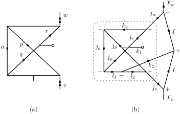
Figure 2: Examples of $E1_{\rm PNC}^{\rm NSD}$ diagrams (a) one of the exchange diagrams in electronic sector and (b) angular momentum diagram in terms of hyperfine states and the portion within the dash lines is the electronic component.

To demonstrate the non-trivial angular integration, in hyperfine atomic states, the angular momentum diagram of the same diagram is shown in Fig. 2(b). Conventions of phase and angular momentum lines of Lindgren and Morrison lindgren-85 are used while drawing the diagram. The portion of the diagram within the rectangle in dashed-line is the angular momentum part of the electronic sector. The evaluation of the angular integral of the electronic sector, following Wigner-Eckert theorem, is equivalent to

$$\langle j_{w}m_{w}|\sum_{l}\left\{{T_{2}^{(0)}}^{\dagger}\mathbf{D}\mathbf{S}^{(1)}_{1}\right\}^{l}|j_{v}m_{v}\rangle=(-1)^{j_{w}-m_{w}}$$

$$\times\sum_{l}\left(\begin{array}[]{ccc}j_{w}&l&j_{v}\\ -m_{w}&q&m_{v}\end{array}\right)\langle j_{w}|\!|\left\{{T_{2}^{(0)}}^{\dagger}\mathbf{D}\mathbf{S}^{(1)}_{1}\right\}^{l}|\!|j_{v}\rangle,$$ (14)

where $\{\ldots\}^{l}$ represents coupling of rank one tensor operators $\mathbf{D}$ and $\mathbf{S}^{(1)}$ to an operator of rank $l$. This coupling is a structure common to any PRCC term of $E1_{\rm elec}^{\rm NSD}$. From the triangular condition, $l=0,1,2$ are the allowed values, however, what values of $l$ contribute depends on $j_{v}$ and $j_{w}$. For example, $l=0,1$ contribute in the PNC $6\;^{2}S_{1/2}\rightarrow 7\;^{2}S_{1/2}$ transition of atomic Cs wood-97 , where as only $l=2$ contributes to the proposed PNC $6\;^{2}S_{1/2}\rightarrow 5\;^{2}D_{5/2}$ transition in Ba⁺ fortson-93 .

The angular momentum diagram in Fig. 2(b), after evaluation, reduces to a $9j$-symbol and free line part. Algebraically, the matrix element in the hyperfine states is

$$\sum_{l}\langle F_{w}m_{w}|\left\{\left[{T_{2}^{(0)}}^{\dagger}\mathbf{D}\mathbf{S}^{(1)}_{1}\right]^{l}\mathbf{I}\right\}^{1}|F_{v}m_{v}\rangle=(-1)^{F_{w}-m_{w}}$$

$$\times\left(\begin{array}[]{ccc}F_{w}&1&F_{v}\\ -m_{w}&q&m_{v}\end{array}\right)\langle F_{w}|\!|D_{\rm eff}|\!|F_{v}\rangle,$$ (17)

where $D_{\rm eff}=\sum_{l}\{[{T_{2}^{(0)}}^{\dagger}\mathbf{D}\mathbf{S}^{(1)}_{1}]^{l}\mathbf{I}\}^{1},$ is the effective dipole operator in the hyperfine states. As seen from the angular momentum diagram, coupling of angular momenta in proper sequence is essential to obtain correct angular factors. However, the sequence is not manifest in the algebraic expression.

Table 1: Reduced matrix element, $E1_{\rm PNC}^{\rm NSD}$, of the $6\;^{2}S_{1/2}\rightarrow 7\;^{2}S_{1/2}$, $6\;^{2}S_{1/2}\rightarrow 5\;^{2}D_{3/2}$ and $7\;^{2}S_{1/2}\rightarrow 6\;^{2}D_{3/2}$ transitions between different hyperfine states in Cs, Ba⁺ and Ra⁺ respectively. The values listed are in units of $iea_{0}\times 10^{-12}\mu^{\prime}_{W}$.

Atom	Transition		This work			Other works
	$F_{f}$	$F_{i}$	DF	MBPT	PRCC
133Cs	3	3	$2.011$	$2.060$	$2.274$	$2.249$ johnson-03
	4	4	$2.289$	$2.338$	$2.589$	$2.560$ johnson-03
	4	3	$5.000$	$4.819$	$5.446$	$6.432$ johnson-03 ,
						$7.057$ safronova-09
	3	4	$5.774$	$5.662$	$6.313$	$7.299$ johnson-03 ,
						$7.948$ safronova-09
135Ba+	3	2	$-2.716$	$-2.881$	$-2.404$	$-2.915$ sahoo-11 ,
						$-2.565$ dzuba-11
	2	1	$2.707$	$2.834$	$1.607$	$2.682$ sahoo-11 ,
						$2.430$ dzuba-11
139Ba+	3	3	$-7.060$	$-6.884$	$-4.951$	$-7.250$ sahoo-11
						$-6.510$ dzuba-11
	2	3	$6.888$	$7.386$	$6.096$	$7.389$ sahoo-11 ,
						$6.510$ dzuba-11
225Ra+	2	1	$-8.568$	$-9.084$	$-8.125$	$-9.918$ sahoo-11 ,
						$-8.90$ dzuba-11
223Ra+	3	2	$-30.414$	$-32.513$	$-28.840$	$-35.204$ sahoo-11 ,
						$-31.65$ dzuba-11
	2	1	$30.307$	$32.286$	$15.683$	$30.525$ sahoo-11 ,
						$24.15$ dzuba-11
229Ra+	2	3	$-20.217$	$-21.788$	$1.137$	$-16.297$ sahoo-11
	3	2	$47.336$	$50.917$	$20.614$	$-9.50$ dzuba-11
	2	2	$-52.906$	$-53.404$	$-38.558$	$-57.387$ sahoo-11 ,
						$-49.00$ dzuba-11

Table 2: Component wise contribution from the coupled-cluster terms for $6\;^{2}S_{1/2}\rightarrow 7\;^{2}S_{1/2}$ transition in Cs, $6\;^{2}S_{1/2}\rightarrow 5\;^{2}D_{3/2}$ transition in Ba⁺, and $7\;^{2}S_{1/2}\rightarrow 6\;^{2}D_{3/2}$ transition in Ra⁺.

Atom	Transition		$DS^{(1)}_{1}$	${S^{(1)}_{1}}^{\dagger}D$	$DT^{(1)}_{1}$	${S^{(0)}}^{\dagger}DS^{(1)}_{1}$
	$F_{f}$	$F_{i}$			$+$ c.c.	$+$ c.c.
133Cs	$3$	$3$	$-0.278$	$4.198$	$-0.005$	$-1.533$
	$4$	$4$	$-0.317$	$4.779$	$-0.006$	$-1.746$
	$4$	$3$	$0.764$	$6.385$	$-0.486$	$-0.531$
	$3$	$4$	$0.657$	$8.001$	$-0.488$	$-1.121$
135Ba+	$3$	$2$	$-2.676$	$0.590$	$-0.647$	$-0.301$
	$2$	$1$	$2.566$	$-0.723$	$0.603$	$-0.276$
139Ba+	$3$	$3$	$-6.808$	$1.729$	$-1.620$	$0.747$
	$2$	$3$	$6.784$	$-1.496$	$1.639$	$-0.763$

Results.—For the calculations reported in the letter, we use Gaussian type orbitals generated with $V^{N-1}$ central potential. The $E1_{\rm PNC}^{\rm NSD}$ of Cs, Ba⁺ and Ra⁺ between various hyperfine states are given in Table. 1. There is a close match between our MBPT results and results from similar works.

There are changes when the transition amplitudes are calculated with PRCC. This can be attributed to the inclusion of higher order correlation effects. However, it require a systematic series of calculations to examine the nature of the correlation effects from the higher order terms which are subsumed in the PRCC calculations. The results of ²²⁹Ra⁺ is a cause for concern, there is a large cancellation in the $F_{i}=3\rightarrow F_{f}=2$ transition amplitude. However, for the other two transitions of the same ion, the transition amplitudes are higher than Ba⁺. In particular, the $F_{i}=2\rightarrow F_{f}=2$ transition amplitude of ²²⁹Ra⁺ is the largest among all the values and this is in agreement with the previous results. For the neutral atom Cs, the PRCC results are larger than MBPT. This indicates, higher order correlation effects enahances $E1_{\rm PNC}^{\rm NSD}$. It is opposite in Ba⁺ and Ra⁺, the PRCC results are lower than MBPT and indicates higher correlation effects have suppression effect.

To examine the impact of electron correlation in better detail, consider the leading order (LO) and next to leading order (NLO) terms as listed in Table. 2. In the PRCC calculations, as given in Eq. (11), for Cs these are ${\mathbf{S}^{(1)}_{1}}^{\dagger}D$ and $D\mathbf{S}^{(1)}_{1}$, respectively. Here, the former represents $H_{\rm PNC}^{\rm NSD}$ perturbed $7\;^{2}S_{1/2}$ and has larger opposite parity mixing as it is energetically closer to odd parity states like $6\;^{2}P_{1/2}$. The same is not true of $6\;^{2}S_{1/2}$, which is represented by $D\mathbf{S}^{(1)}_{1}$.

In the case of Ba⁺ the LO and NLO are $D\mathbf{S}^{(1)}_{1}$ and ${\mathbf{S}^{(1)}_{1}}^{\dagger}D$, respectively. Although, not shown in Table. 2 a similar pattern is observed in Ra⁺. The sequence is opposite to Cs. Reason is, the transitions in these ions are of $n\;^{2}S_{1/2}\rightarrow n^{\prime}\;{}^{2}D_{3/2}$ type and matrix elements of $H_{\rm PNC}^{\rm NSD}$ involving $n^{\prime}\;{}^{2}D_{3/2}$ are negligible. Dominant contribution arises from the $sp$ matrix elements, which are large. So, the term $D\mathbf{S}^{(1)}_{1}$, which represents $H_{\rm PNC}^{\rm NSD}$ perturbation of $n\;^{2}S_{1/2}$ is the LO term of these ions. The contribution from ${\mathbf{S}^{(1)}_{1}}^{\dagger}D$ is, however, non-zero as $n^{\prime}\;{}^{2}D_{3/2}$ acquires opposite parity mixing through electron correlation effects. It must be mentioned that, the Dirac-Fock contribution is the most dominant, however, in PRCC it is subsumed in the LO and NLO terms. The terms which are second order in cluster operators, in Eq. (11), are non-zero but small. For comparison, the two dominant contributions from the second order term, ${S^{(0)}}^{\dagger}DS^{(1)}_{1}$ and it’s hermitian conjugate, is given in the Table. 2.

Table 3: Reduced matrix element, $E1_{\rm PNC}^{\rm NSD}$, of the $6\;^{2}S_{1/2}\rightarrow 5\;^{2}D_{5/2}$ and $7\;^{2}S_{1/2}\rightarrow 6\;^{2}D_{5/2}$ transitions between different hyperfine states Ba⁺ and Ra⁺ respectively. The values listed are in units of $iea_{0}\times 10^{-12}\mu^{\prime}_{W}$.

Atom	Transition		This work			Other works
	$F_{f}$	$F_{i}$	DF	MBPT	PRCC
135Ba+	$3$	$2$	$0.003$	$0.098$	$0.227$	$0.041$ sahoo-11
	$2$	$1$	$0.002$	$0.048$	$0.127$	$-$
139Ba+	$2$	$3$	$0.003$	$0.125$	$0.235$	$0.043$ sahoo-11
223Ra+	$3$	$2$	$-0.040$	$-0.605$	$1.262$	$-0.526$ sahoo-11
229Ra+	$2$	$3$	$-0.019$	$-0.324$	$0.616$	$-0.256$ sahoo-11

We have also calculated the $E1_{\rm PNC}^{\rm NSD}$ of the $6\;^{2}S_{1/2}\rightarrow 5\;^{2}D_{5/2}$ and $7\;^{2}S_{1/2}\rightarrow 6\;^{2}D_{5/2}$ transitions in Ba⁺ and Ra⁺, respectively, and the results are given in Table. 3. The results from the PRCC are much larger than the MBPT results and this shows, without any ambiguity, electron correlation is the key to get meaningful results. This is on account of $d_{5/2}$ in the atomic $n\;^{2}D_{5/2}$ states, which are diffused and leads to larger electron correlations.

Conclusions.— The PRCC theory we have developed incorporates electron correlation effects arising from a class of diagrams to all order with a nuclear spin-dependent interaction as a perturbation. It is a suitable theory for precision calculations of atomic PNC arising from $H_{\rm PNC}^{\rm NSD}$. With this method, it is possible to incorporate electron correlation effects within the entire configuration space obtained from a set of spin-orbitals.

Acknowledgements.—We thank B. K. Sahoo, S. Chattopadhyay, S. Gautam and S. A. Silotri for valuable discussions. The results presented in the paper are based on computations using the HPC cluster at Physical Research Laboratory, Ahmedabad.

References

(1)
C. S. Wood, et al. Science 275, 1759 (1997).
(2)
Y. Zel’dovich,
JETP 6, 1184 (1958).
(3)
N. Fortson,
Phys. Rev. Lett. 70, 2383 (1993).
(4)
K. Tsigutkin, et al.,
Phys. Rev. Lett. 103, 071601 (2009).
(5)
F. Coester,
Nucl. Phys. 7, 421 (1958).
(6)
F. Coester and H. Kümmel,
Nucl. Phys. 17, 477 (1960).
(7)
G. Hagen, T. Papenbrock, D. J. Dean, and M. Hjorth-Jensen,
Phys. Rev. Lett. 101, 092502 (2008).
(8)
E. Eliav, U. Kaldor, and Y. Ishikawa,
Phys. Rev. A a50, 1121 (1994).
(9)
H. S. Nataraj, B. K. Sahoo, B. P. Das, and D. Mukherjee,
Phys. Rev. Lett. 101, 033002 (2008).
(10)
R. Pal, et al.,
Phys. Rev. A 75, 042515 (2007).
(11)
T. A. Isaev, et al.,
Phys. Rev. A 69, 030501(R) (2004).
(12)
R. F. Bishop, P. H. Y. Li, D. J. J. Farnell, and C. E. Campbell,
Phys. Rev. B 79, 174405 (2009).
(13)
B. K. Sahoo, L. W. Wansbeek, K. Jungmann, and R. G. E. Timmermans,
Phys. Rev. A 79, 052512 (2009).
(14)
C. Thierfelder and P. Schwerdtfeger,
Phys. Rev. A 79, 032512 (2009).
(15)
B. K. Sahoo, B. P. Das, and D. Mukherjee,
Phys. Rev. A 79, 052511 (2009).
(16)
L. W. Wansbeek, et al.,
Phys. Rev. A 78, 050501(R) (2008).
(17)
S. G. Porsev, K. Beloy, and A. Derevianko,
Phys. Rev. D 82, 036008 (2010).
(18)
R. Pal, D. Jiang, M. S. Safronova, and U. I. Safronova,
Phys. Rev. A 79, 062505 (2009).
(19)
B. K. Sahoo, P. Mandal and M. Mukherjee,
Phys. Rev. A 83 , 030502 (2011).
(20)
K. V. P. Latha, D. Angom, B. P. Das, and D. Mukherjee,
Phys. Rev. Lett. 103, 083001 (2009).
(21)
B. K. Mani and D. Angom,
Phys. Rev. A 81, 042514 (2010).
(22)
B. K. Mani and D. Angom,
Phys. Rev. A 83, 012501 (2011).
(23)
B. K. Mani, K. V. P. Latha, and D. Angom,
Phys. Rev. A 80, 062505 (2009).
(24)
B. K. Sahoo, R. Chaudhuri, B. P. Das, and D. Mukherjee,
Phys. Rev. Lett. 96, 163003 (2006).
(25)
I. Lindgren and J. Morrison,
Atomic Many-Body Theory,
edited by G. Ecker, P. Lambropoulos, and H. Walther
(Springer-Verlag, 1985).
(26)
W. R. Johnson, M. S. Safronova, and U. I. Safronova,
Phys. Rev. A 67, 062106 (2003).
(27)
M. S. Safronova et al.,
Nuclear Physics A 827, 411c-413c (2009).
(28)
V. A. Dzuba, V. V. Flambaum,
arXiv:1104.0086.