Principal arc analysis on direct product manifolds

Abstract

We propose a new approach to analyze data that naturally lie on manifolds. We focus on a special class of manifolds, called direct product manifolds, whose intrinsic dimension could be very high. Our method finds a low-dimensional representation of the manifold that can be used to find and visualize the principal modes of variation of the data, as Principal Component Analysis (PCA) does in linear spaces. The proposed method improves upon earlier manifold extensions of PCA by more concisely capturing important nonlinear modes. For the special case of data on a sphere, variation following nongeodesic arcs is captured in a single mode, compared to the two modes needed by previous methods. Several computational and statistical challenges are resolved. The development on spheres forms the basis of principal arc analysis on more complicated manifolds. The benefits of the method are illustrated by a data example using medial representations in image analysis.

, and

1 Introduction

Principal Component Analysis (PCA) has been frequently used as a method of dimension reduction and data visualization for high-dimensional data. For data that naturally lie in a curved manifold, application of PCA is not straightforward since the sample space is not linear. Nevertheless, the need for PCA-like methods is growing as more manifold data sets are encountered and as the dimensions of the manifolds increase.

In this article we introduce a new approach for an extension of PCA on a special class of manifold data. We focus on direct products of simple manifolds, in particular, of the unit circle $S^{1}$, the unit sphere $S^{2}$, $\mathbb{R}_{+}$ and $\mathbb{R}^{p}$. We will refer to these as direct product manifolds, for convenience. Many types of statistical sample spaces are special cases of the direct product manifold. A widely known example is the sample space for directional data [Fisher (1993), Fisher, Lewis and Embleton (1993) and Mardia and Jupp (2000)] and their direct products. Applications include analysis of wind directions, orientations of cracks, magnetic field directions and directions from the earth to celestial objects. For example, when we consider multiple 3-D directions simultaneously, the sample space is $S^{2}\otimes\cdots\otimes S^{2}$, which is a direct product manifold. Another example is the medial representation of shapes [m-reps, Siddiqi and Pizer (2008)], which is somewhat less known to the statistical community but provides a powerful parametrization of 3-D shapes of human organs and has been extensively studied in the image analysis field. The space of m-reps is usually a high-dimensional direct product manifold. Some background and necessary definitions on direct product manifolds can be found in Appendix.

Our approach to a manifold version of PCA builds upon earlier work, especially the principal geodesic analysis proposed by Fletcher et al. (2004) and the geodesic PCA proposed by Huckemann and Ziezold (2006) and Huckemann, Hotz and Munk (2010). A detailed catalogue of current methodologies can be found in Huckemann, Hotz and Munk (2010). An important approach among these is to approximate the manifold by a linear space. Fletcher et al. (2004) take the tangent space of the manifold at the geodesic mean as the linear space, and work with appropriate mappings between the manifold and the tangent space. This results in finding the best fitting geodesics among those passing through the geodesic mean. This was improved in an important way by Huckemann, Hotz and Munk, who found the best fit over the set of all geodesics. Huckemann, Hotz and Munk went on to propose a new notion of center point, the PCmean, which is an intersection of the first two principal geodesics. This approach gives significant advantages, especially when the curvature of the manifold makes the geodesic mean inadequate, an example of which is depicted in Figure 2b.

Our method inherits advantages of these methods and improves further by effectively capturing more complex nongeodesic modes of variation. Note that the curvature of direct product manifolds is mainly due to the spherical part, which motivates careful investigation of $S^{2}$-valued variables. We point out that (small) circles in $S^{2}$, including geodesics, can be used to capture the nongeodesic variation. We introduce the principal circles and principal circle mean, analogous to, yet more flexible than, the geodesic principal component and PCmean of Huckemann, Hotz and Munk. These become principal arcs when the manifold is indeed $S^{2}$. For more complex direct product manifolds, we suggest transforming the data points in $S^{2}$ into a linear space by a special mapping utilizing the principal circles. For the other components of the manifold, the tangent space mappings can be used to map the data into a linear space as done in Fletcher et al. (2004). Once manifold-valued data are mapped onto the linear space, then the classical linear PCA can be applied to find principal components in the transformed linear space. The estimated principal components in the linear space can be back-transformed to the manifold, which leads to principal arcs.

We illustrate the potential of our method by an example of m-rep data in Figure 1. Here, m-reps with 15 sample points called atoms model the prostate gland (an organ in the male reproductive system) and come from the simulator developed and analyzed in Jeong et al. (2008). Figure 1 shows that the $S^{2}$ components of the data tend to be distributed along small circles, which frequently are not geodesics. We emphasize the curvature of variation along each sphere by fitting a great circle and a small circle (by the method discussed in Section 2). Our method is adapted to capture this nonlinear (nongeodesic) variation of the data. A potential application of our method is to improve accuracy of segmentation of objects from CT images. Detailed description of the data and results of our analysis can be found in Section 5.

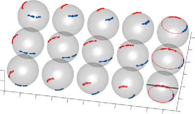
Figure 1: $S^{2}$-valued samples ($n=60$) of the prostate m-reps with 15 medial atoms. One sample in this figure is represented by a 30-tuple of 3-D directions (two directions at each atom), which lies in the manifold $\bigotimes_{i=1}^{15}(S^{2}\otimes S^{2})$. Small and great circles are fitted and plotted in the rightmost atoms to emphasize the sample variation along small circles.

Note that the previous approaches [Fletcher et al. (2004), Huckemann and Ziezold (2006)] are defined for general manifolds, while our method focuses on these particular direct product manifolds. Although the method is not applicable for general manifolds, it is useful for this common class of manifolds that is often found in applications. Our results inform our belief that focusing on specific types of manifolds allow more precise and informative statistical modeling than methods that attempt to be fully universal. This happens through using special properties (e.g., presence of small circles) that are not available for all other manifolds.

The rest of the article is organized as follows. We begin by introducing a circle class on $S^{2}$ as an alternative to the set of geodesics. Section 2 discusses principal circles in $S^{2}$, which will be the basis of the special transformation. The first principal circle is defined by the least-squares circle, minimizing the sum of squared residuals. In Section 3 we introduce a data-driven method to decide whether the least-squares circle is appropriate. A recipe for principal arc analysis on direct product manifolds is proposed in Section 4 with discussion on the transformations. A detailed introduction of the space of m-reps and the results from applying the proposed method follow. A novel computational algorithm for the least-squares circles is presented in Section 6. In the Appendix we provide some necessary background for treating direct product manifolds as sample spaces, including the notion of geodesic mean, tangent space, exponential map and log map.

2 Circle class for nongeodesic variation on $S^{2}$

Consider a set of points in $\mathbb{R}^{2}$. Numerous methods for understanding population properties of a data set in linear space have been proposed and successfully applied, which include rigid methods, such as linear regression and principal components, and very flexible methods, such as scatterplot smoothing and principal curves [Hastie and Stuetzle (1989)]. In this paper we make use of a parametric class of circles, including small and great circles, which allows much more flexibility than either methods of Fletcher et al. (2004) or Huckemann, Hotz and Munk (2010), but less flexibility than a principal curve approach. Although this idea was motivated by examples such as those in Figure 1, there are more advantages gained from using the class of circles:

1. [(iii)]

2. The circle class includes the simple geodesic case.

3. Each circle can be parameterized, which leads to an easy interpretation.

4. There is an orthogonal complement of each circle, which gives two important advantages:

   1. [(a)]

   2. Two orthogonal circles can be used as a basis of a further extension to principal arc analysis.

   3. Building a sensible notion of principal components on $S^{2}$ alone is easily done by utilizing the circles.

The idea (iii)(b) will be discussed in detail after introducing a method of circle fitting. Some notations follow: $S^{2}$ can be thought of as the unit sphere in $\mathbb{R}^{3}$, so that a unit vector $\mathbf{x}\in\mathbb{R}^{3}$ is a member of $S^{2}$. The geodesic distance between $\mathbf{x},\mathbf{y}\in S^{2}$, denoted by $\rho(\mathbf{x},\mathbf{y})$, is defined as the shortest distance between $\mathbf{x}$, $\mathbf{y}$ along the sphere, which is the same as the angle formed by the two vectors. Thus, $\rho(\mathbf{x},\mathbf{y})=\cos^{-1}(\mathbf{x}^{\prime}\mathbf{y})$. A circle on $S^{2}$ is conveniently parameterized by center $\mathbf{c}\in S^{2}$ and geodesic radius $r$, and denoted by $\delta(\mathbf{c},r)=\{\mathbf{x}\in S^{2}|\rho(\mathbf{c},\mathbf{x})=r\}$. It is a geodesic when $r=\pi/2$. Otherwise it is a small circle.

A circle that best fits the points $\mathbf{x}_{1},\ldots,\mathbf{x}_{n}\in S^{2}$ is found by minimizing the sum of squared residuals. The residual of $\mathbf{x}_{i}$ is defined as the signed geodesic distance from $\mathbf{x}_{i}$ to the circle $\delta(\mathbf{c},r)$. Then the least-squares circle is obtained by

$$\min_{\mathbf{c},r}\sum_{i=1}^{n}\bigl{(}\rho(\mathbf{x}_{i},\mathbf{c})-r\bigr{)}^{2}\qquad\mbox{subject to }\mathbf{c}\in S^{2},r\in(0,\pi).$$ (1)

Note that there are always multiple solutions of (1). In particular, whenever $(\mathbf{c},r)$ is a solution, $(-\mathbf{c},\pi-r)$ also solves the problem as $\delta(\mathbf{c},r)=\delta(-\mathbf{c},\pi-r)$. This ambiguity does not affect any essential result in this paper. Our convention is to use the circle with smaller geodesic radius.

The optimization task (1) is a constrained nonlinear least squares problem. We propose an algorithm to solve the problem that features a simplified optimization task and approximation of $S^{2}$ by tangent planes. The algorithm works in a doubly iterative fashion, which has been shown by experience to be stable and fast. Section 6 contains a detailed illustration of the algorithm.

Analogous to principal geodesics in $S^{2}$, we can define principal circles in $S^{2}$ by utilizing the least-squares circle. The principal circles are two orthogonal circles in $S^{2}$ that best fit the data. We require the first principal circle to minimize the variance of the residuals, so it is the least-squares circle (1). The second principal circle is a geodesic which passes through the center of the first circle and thus is orthogonal at the points of intersection. Moreover, the second principal circle is chosen so that one intersection point is the intrinsic mean [defined in (2) later] of the projections of the data onto the first principal circle.

Based on a belief that the intrinsic (or extrinsic) mean defined on a curved manifold may not be a useful notion of the center point of the data [see, e.g., Huckemann, Hotz and Munk and Figure 2b], the principal circles do not use the pre-determined means. To develop a better notion of center point, we locate the best 0-dimensional representation of the data in a data-driven manner. Inspired by the PCmean idea of Huckemann, Hotz and Munk, given the first principal circle $\delta_{1}$, the principal circle mean $\mathbf{u}\in\delta_{1}$ is defined (in an intrinsic way) as

$$\mathbf{u}=\mathop{\mathrm{argmin}}_{\mathbf{u}\in\delta_{1}}\sum_{i=1}^{n}\rho^{2}(\mathbf{u},P_{\delta_{1}}\mathbf{x}_{i}),$$ (2)

where $P_{\delta_{1}}\mathbf{x}$ is the projection of $\mathbf{x}$ onto $\delta_{1}$, that is, the point on $\delta_{1}$ of the shortest geodesic distance to $\mathbf{x}$. Then

$$P_{\delta_{1}(\mathbf{c},r)}\mathbf{x}=\frac{\mathbf{x}\sin(r)+\mathbf{c}\sin(\rho(\mathbf{x},\mathbf{c})-r)}{\sin(\rho(\mathbf{x},\mathbf{c}))},$$ (3)

as in equation (3.3) of Mardia and Gadsden (1977). We assume that $\mathbf{c}$ is the north pole $\mathbf{e}_{3}$, without losing generality since otherwise the sphere can be rotated. Then

$$\rho(\mathbf{u},P_{\delta_{1}}\mathbf{x})=\sin(r)\rho_{S^{1}}\biggl{(}\frac{(u_{1},u_{2})}{\sqrt{1-u_{3}^{2}}},\frac{(x_{1},x_{2})}{\sqrt{1-x_{3}^{2}}}\biggr{)},$$ (4)

where $\mathbf{u}=(u_{1},u_{2},u_{3})^{\prime}$, $\mathbf{x}=(x_{1},x_{2},x_{3})^{\prime}$ and $\rho_{S^{1}}$ is the geodesic (angular) distance function on $S^{1}$. The optimization problem (2) is equivalent to finding the geodesic mean in $S^{1}$. See equation (17) in the Appendix for computation of the geodesic mean in $S^{1}$.

The second principal circle $\delta_{2}$ is then the geodesic passing through the principal circle mean $\mathbf{u}$ and the center $\mathbf{c}$ of $\delta_{1}$. Denote $\bar{\delta}\equiv\bar{\delta}(\mathbf{x}_{1},\ldots,\mathbf{x}_{n})$ as a combined representation of $(\delta_{1},\mathbf{u})$ or, equivalently, $(\delta_{1},\delta_{2})$.

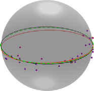
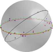
(a)	(b)
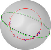
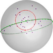
(c)	(d)

Figure 2: Toy examples on $S^{2}$ with $n=30$ points showing the first principal circle (red) as a small circle and the first geodesic principal component (dotted green) by Huckemann, and the first principal geodesic (black) by Fletcher. Also plotted are the geodesic mean, PCmean and principal circle mean of the data as black, green and red diamonds, respectively. (a) The three methods give similar satisfactory answers when the data are stretched along a geodesic. (b) When the data are stretched along a great circle, covering almost all of it, the principal geodesic (black circle) and geodesic mean (black diamond) fail to find a reasonable representation of the data, while the principal circle and Huckemann’s geodesic give sensible answers. (c) Only the principal circle fits well when the data are not along a geodesic. (d) For a small cluster without principal modes of variation, the principal circle gets too small. See Section 3 for discussion of this phenomenon.

As a special case, we can force the principal circles to be great circles. The best fitting geodesic is obtained as a solution of the problem (1) with $r=\pi/2$ and becomes the first principal circle. The optimization algorithm for this case is slightly modified from the original algorithm for the varying $r$ case by simply setting $r=\pi/2$. The principal circle mean $\mathbf{u}$ and the $\delta_{2}$ for this case are defined in the same way as in the small circle case. Note that the principal circles with $r=\pi/2$ are essentially the same as the method of Huckemann and Ziezold (2006).

Figure 2 illustrates the advantages of using the circle class to efficiently summarize variation. On four different sets of toy data, the first principal circle $\delta_{1}$ is plotted with principal circle mean $\mathbf{u}$. The first principal geodesics from the methods of Fletcher and Huckemann are also plotted with their corresponding mean. Figure 2a illustrates the case where the data were indeed stretched along a geodesic. The solutions from the three methods are similar to one another. The advantage of Huckemann’s method over Fletcher’s can be found in Figure 2b. The geodesic mean is found far from the data, which leads to poor performance of the principal geodesic analysis, because it considers only great circles passing through the geodesic mean. Meanwhile, the principal circle and Huckemann’s method, which do not utilize the geodesic mean, work well. The case where geodesic mean and any geodesic do not fit the data well is illustrated in Figure 2c, which is analogous to the Euclidean case, where a nonlinear fitting may do a better job of capturing the variation than PCA. To this data set, the principal circle fits best, and our definition of mean is more sensible than the geodesic mean and the PCmean. The points in Figure 2d are generated from the von Mises–Fisher distribution with $\kappa=10$, thus having no principal mode of variation. In this case the first principal circle $\delta_{1}$ follows a contour of the apparent density of the points. We shall discuss this phenomenon in detail in the following section.

Fitting a (small) circle to data on a sphere has been investigated for some time, especially in statistical applications in geology. Those approaches can be distinguished in three different ways, where our choice fits into the first category:

1. [(2)]

2. Least-squares of intrinsic residuals: Gray, Geiser and Geiser (1980) formulated the same problem as in (1), finding a circle that minimizes sum of squared residuals, where residuals are defined in a geodesic sense.

3. Least-squares of extrinsic residuals: A different measure of residual was chosen by Mardia and Gadsden (1977) and Rivest (1999), where the residual of $\mathbf{x}$ from $\delta(c,r)$ is defined by the shortest Euclidean distance between $\mathbf{x}$ and $\delta(\mathbf{c},r)$. Their objective is to find

   $$\mathop{\mathrm{argmin}}_{\delta}\sum_{i=1}^{n}\|\mathbf{x}_{i}-P_{\delta}\mathbf{x}_{i}\|^{2}=\mathop{\mathrm{argmin}}_{\delta}\sum_{i=1}^{n}-\mathbf{x}_{i}^{\prime}P_{\delta}\mathbf{x}_{i}=\mathop{\mathrm{argmin}}_{\delta}\sum_{i=1}^{n}-\cos(\xi_{i}),$$

   where $\xi_{i}$ denotes the intrinsic residual. This type of approach can be numerically close to the intrinsic method as $\cos(\xi_{i})=1-\xi_{i}^{2}/2+O(\xi_{i}^{4})$.

4. Distributional approach: Mardia and Gadsden (1977) and Bingham and Mardia (1978) proposed appropriate distributions to model $S^{2}$-valued data that cluster near a small circle. These models essentially depend on the quantity $\cos(\xi)$, which is easily interpreted in the extrinsic sense but not in the intrinsic sense.

The principal circle and principal circle mean always exist. This is because the objective function (1) is a continuous function of $\mathbf{c}$, with the compact domain $S^{2}$. The minimizer $r$ has a closed-form solution (see Section 6). A similar argument can be made for the existence of $\mathbf{u}$. On the other hand, the uniqueness of the solution is not guaranteed. We conjecture that if the manifold is approximately linear or, equivalently, the data set is well approximated by a linear space, then the principal circle will be unique. However, this does not lead to the uniqueness of $\mathbf{u}$, whose sufficient condition is that the projected data on $\delta_{1}$ is strictly contained in a half-circle [Karcher (1977)]. Note that a sufficient condition for the uniqueness of the principal circle is not clear even in the Euclidean case [Chernov (2010)].

3 Suppressing small least-squares circles

When the first principal circle $\delta_{1}$ has a small radius, sometimes it is observed that $\delta_{1}$ does not fit the data in a manner that gives useful decomposition, as shown in Figure 2d. This phenomenon has been also observed for the related principal curve fitting method of Hastie and Stuetzle (1989). We view this as unwanted overfitting, which is indeed a side effect caused by using the full class of circles with free radius parameter instead a class of great circles. In this section a data-driven method to flag this overfitting is discussed. In essence, the fitted small circle is replaced by the best fitting geodesics when the data do not cluster along the circle but instead tend to cluster near the center of the circle.

We first formulate the problem and solution in $\mathbb{R}^{2}$. This is for the sake of clear presentation and also because the result on $\mathbb{R}^{2}$ can be easily extended to $S^{2}$ using a tangent plane approximation.

Let $f_{\mathbf{X}}$ be a spherically symmetric density function of a continuous distribution defined on $\mathbb{R}^{2}$. Whether the density is high along some circle is of interest. By the symmetry assumption, density height along a circle can be found by inspecting a section of $f_{\mathbf{X}}$ along a ray from the origin (the point of symmetry). A section of $f_{\mathbf{X}}$ coincides with the conditional density $f_{X_{1}|X_{2}}(x_{1}|x_{2}=0)=\kappa^{-1}f_{\mathbf{X}}(x_{1},0)$. A random variable corresponding to the p.d.f. $f_{X_{1}|X_{2}=0}$ is not directly observable. Instead, the radial distance $R=\|\mathbf{X}\|$ from the origin can be observed. For the polar coordinates $(R,\Theta)$ such that $\mathbf{X}=(X_{1},X_{2})=(R\cos\Theta,R\sin\Theta)$, the marginal p.d.f. of $R$ is $f_{R}(r)=2\pi rf_{\mathbf{X}}(r,0)$ as $f_{\mathbf{X}}$ is spherically symmetric. A section of $f_{\mathbf{X}}$ is related to the observable density $f_{R}$ as $f_{R}(r)\propto rf_{X_{1}|X_{2}=0}(r)$, for $r\geq 0$. This relation is called the length-biased sampling problem [Cox (1969)]. The relation can be understood intuitively by observing that a value $r$ of $R$ can be observed at any point on a circle of radius $r$, circumference of which is proportional to $r$. Thus, sampling of $R$ from the density $f_{X_{1}|X_{2}=0}$ is proportional to its size.

The problem of suppressing a small circle can be paraphrased as “how to determine whether a nonzero point is a mode of the function $f_{X_{1}|X_{2}=0}$, when observing only a length-biased sample.”

The spectrum from the circle-clustered case (mode at a nonzero point) to the center-clustered case (mode at origin) can be modeled as

$$\mathrm{data}=\mathrm{signal}+\mathrm{error},$$ (5)

where the signal is along a circle with radius $\mu$, and the error accounts for the perpendicular deviation from the circle (see Figure 3). Then, in polar coordinates $(R,\Theta)$, $\Theta$ is uniformly distributed on $(0,2\pi]$ and $R$ is a positive random variable with mean $\mu$. First assume that $R$ follows a truncated Normal distribution with standard deviation $\sigma$, with the marginal p.d.f. proportional to

$$f_{R}(r)\propto\phi\biggl{(}\frac{r-\mu}{\sigma}\biggr{)}\qquad\mbox{for }r\geq 0,$$ (6)

where $\phi$ is the standard Normal density function. The conditional density $f_{X_{1}|X_{2}=0}$ is then

$$f_{X_{1}|X_{2}=0}(r)\propto\frac{1}{r}f_{R}(r)\propto\frac{1}{r\sigma}\exp\biggl{(}-\frac{(r-\mu)^{2}}{\sigma^{2}}\biggr{)}\qquad\mbox{for }r>0.$$

Nonzero local extrema of $f_{X_{1}|X_{2}=0}$ can be characterized as a function of $(\mu,\sigma)$ in terms of $r_{+},r_{-}=\{\mu\pm\sqrt{(\mu-2\sigma)(\mu+2\sigma)}\}/2$ as follows:

• When $\mu>2\sigma$, $f_{X_{1}|X_{2}=0}$ has a local maximum at $r_{+}$, minimum at $r_{-}$.

• When $\mu=2\sigma$, $r_{+}=r_{-}=\frac{\mu}{2}.$

• When $\mu<2\sigma$, $f_{X_{1}|X_{2}=0}$ is strictly decreasing, for $r\geq 0$.

Therefore, whenever the ratio $\mu/\sigma>2$, $f_{X_{1}|X_{2}=0}$ has a mode at $r_{+}$.

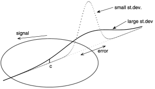
Figure 3: Illustration of the conceptual model (5) on $\mathbb{R}^{2}$, which can also be understood as a local approximation of $S^{2}$. The signal is along the circle centered at $c$ and radius $\mu$. The error is perpendicular to the signal. When the deviation $\sigma$ is large, it is possible that the amount of error is even greater than the radius $\mu$. This is incorporated in the wrapping approach (7).

This idea can be applied for circles in $S^{2}$ with some modification, shown next. We point out that the model (5) is useful for understanding the small circle fitting: signal as a circle with radius $\mu$, and error as the deviation along geodesics perpendicular to the circle. Moreover, a spherically symmetric distribution centered at $\mathbf{c}$ on $S^{2}$ can be mapped to a spherically symmetric distribution on the tangent space at $\mathbf{c}$, preserving the radial distances by the log map (defined in the Appendix). A modification needs to be made on the truncated density $f_{R}$. It is more natural to let the error be so large that the deviation from the great circle is greater than $\mu$. Then the observed value may be found near the opposite side of the true signal, which is illustrated in Figure 3 as the large deviation case. To incorporate this case, we consider a wrapping approach. The distribution of errors (on the real line) is wrapped around the sphere along a great circle through $\mathbf{c}$, and the marginal p.d.f. $f_{R}$ in (6) is modified to

$$\hskip 20.0ptf_{R}^{w}(r)\propto\sum_{k=0}^{\infty}\biggl{[}\phi\biggl{(}\frac{r+2\pi k-\mu}{\sigma}\biggr{)}+\phi\biggl{(}\frac{r-2\pi k+\mu}{\sigma}\biggr{)}\biggr{]}\qquad\mbox{for }r\in[0,\pi].$$ (7)

The corresponding conditional p.d.f., $f_{X_{1}|X_{2}=0}^{w}$, is similar to $f_{X_{1}|X_{2}=0}$ and a numerical calculation shows that $f_{X_{1}|X_{2}=0}^{w}$ has a mode at some nonzero point whenever $\mu/\sigma>2.0534$, for $\mu<\pi/2$. In other words, we use the small circle when $\mu/\sigma$ is large. Note that in what follows we only consider the first term ($k=0$) of (7) since other terms are negligible in most situations. We have plotted $f_{X_{1}|X_{2}=0}^{w}$ for some selected values of $\mu$ and $\sigma$ in Figure 4.

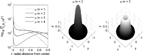
Figure 4: (Left) Graph of $f_{X_{1}|X_{2}=0}^{w}(r)$ for $\mu/\sigma=1,2,3,4$. The density is high at a nonzero point when $\mu/\sigma>2.0534$. (Center, right) Spherically symmetric distributions $f$ corresponding to $\mu/\sigma=2,3$. The ratio $\mu/\sigma>2$ roughly leads to a high density along a circle.

With a data set on $S^{2}$, we need to estimate $\mu$ and $\sigma$, or the ratio $\mu/\sigma$. Let $\mathbf{x}_{1},\ldots,\mathbf{x}_{n}\in S^{2}$ and let $\hat{\mathbf{c}}$ be the samples and the center of the fitted circle, respectively. Denote $\xi_{i}$ for the errors of the model (5) such that $\xi_{i}\sim N(0,\sigma^{2})$. Then $r_{i}\equiv\rho(\mathbf{x}_{i},\hat{\mathbf{c}})=|\mu+\xi_{i}|$, which has the folded normal distribution [Leone, Nelson and Nottingham (1961)]. Estimation of $\mu$ and $\sigma$ based on unsigned $r_{i}$ is not straightforward. We present two different approaches to this problem.

Robust approach. The observations $r_{1},\ldots,r_{n}$ can be thought of as a set of positive numbers contaminated by the folded negative numbers. Therefore, the left half (near zero) of the data are more contaminated than the right half. We only use the right half of the data, which are less contaminated than the other half. We propose to estimate $\mu$ and $\sigma$ by

$$\hat{\mu}=\operatorname{med}(r_{1}^{n}),\qquad\hat{\sigma}=\bigl{(}\mbox{Q}_{3}(r_{1}^{n})-\operatorname{med}(r_{1}^{n})\bigr{)}/\mbox{Q}_{3}(\Phi),$$ (8)

where $\mbox{Q}_{3}(\Phi)$ is the third quantile of the standard normal distribution. The ratio can be estimated by $\hat{\mu}/\hat{\sigma}$.

Likelihood approach via EM algorithm. The problem may also be solved by a likelihood approach. Early solutions can be found in Leone, Nelson and Nottingham (1961), Elandt (1961) and Johnson (1962), in which the MLEs were given by numerically solving nonlinear equations based on the sample moments. As those methods were very complicated, we present a simpler approach based on the EM algorithm. Consider unobserved binary variables $s_{i}$ with values $-1$ and $+1$ so that $s_{i}r_{i}\sim N(\mu,\sigma^{2})$. The idea of the EM algorithm is that if we have observed $s_{i}$, then the maximum likelihood estimator of $\vartheta=(\mu,\sigma^{2})$ would be easily obtained. The EM algorithm is an iterative algorithm consisting of two steps. Suppose that the $k$th iteration produced an estimate $\hat{\vartheta}_{k}$ of $\vartheta$. The E-step is to impute $s_{i}$ based on $r_{i}$ and $\hat{\vartheta}_{k}$ by forming a conditional expectation of log-likelihood for $\vartheta$,

$$Q(\vartheta) = E\Biggl{[}\log\prod_{i=1}^{n}f(r_{i},s_{i}|\vartheta)\Big{|}r_{i},\hat{\vartheta}_{k}\Biggr{]}$$

$$= \sum_{i=1}^{n}\bigl{[}\log f(r_{i}|s_{i}=+1,\vartheta)P(s_{i}=+1|r_{i},\hat{\vartheta}_{k})$$

$$\hskip 17.0pt{}+\log f(r_{i}|s_{i}=-1,\vartheta)P(s_{i}=-1|r_{i},\hat{\vartheta}_{k})\bigr{]}$$

$$= \sum_{i=1}^{n}\bigl{[}\log\phi(r_{i}|\vartheta)p_{i(k)}+\log\phi(-r_{i}|\vartheta)\bigl{(}1-p_{i(k)}\bigr{)}\bigr{]},$$

where $f$ is understood as an appropriate density function, and $p_{i(k)}$ is easily computed as

$$p_{i(k)}=P(s_{i}=+1|r_{i},\hat{\vartheta}_{k})=\frac{\phi(r_{i}|\hat{\vartheta}_{k})}{\phi(r_{i}|\hat{\vartheta}_{k})+\phi(-r_{i}|\hat{\vartheta}_{k})}.$$

The M-step is to maximize $Q(\vartheta)$ whose solution becomes the next estimator $\hat{\vartheta}_{k+1}$. Now the $(k+1)$th estimates are calculated by a simple differentiation and given by

$$\hat{\mu}_{k+1}=\frac{1}{n}\sum_{i=1}^{n}\bigl{(}2p_{i(k)}-1\bigr{)}r_{i},\qquad\hat{\sigma}^{2}_{k+1}=\frac{1}{n}\sum_{i=1}^{n}(r_{i}^{2}-\hat{\mu}_{k+1}^{2}).$$

With the sample mean and variance of $r_{1},\ldots,r_{n}$ as an initial estimator $\hat{\vartheta}_{0}$, the algorithm iterates E-steps and M-steps until the iteration changes the estimates less than a predefined criteria (e.g., $10^{-10}$). $\mu/\sigma$ is estimated by the ratio of the solutions.

Table 1: Proportion of estimates greater than $2$ from the data illustrated in Figure 5. For $\mu/\sigma=3$, shown are proportions of correct answers from each estimator. For $\mu/\sigma=1$ or 0, shown are proportions of incorrect answers

Method	$\bolds{\mu/\sigma=3}$	$\bolds{\mu/\sigma=2}$	$\bolds{\mu/\sigma=1}$	$\bolds{\mu/\sigma=0}$
MLE, $n=50$	$98.5$	$55.2$	$5.2$	$6.8$
Robust, $n=50$	$95.0$	$50.5$	$4.7$	$1.4$
MLE, $n=1000$	$100$	$51.9$	$0$	$0$
Robust, $n=1000$	$100$	$50.5$	$0$	$0$

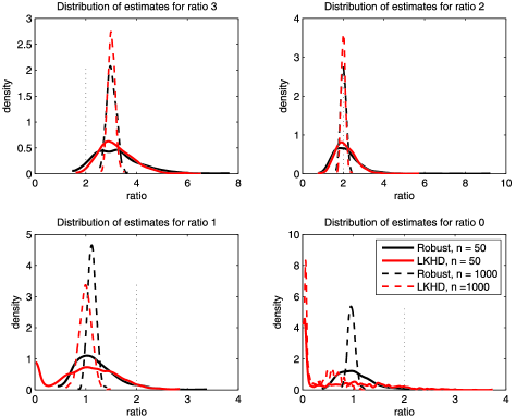
Figure 5: Simulation results of the proposed estimators for the ratio $\mu/\sigma$. Different ratios represent different underlying distributions. For example, estimators in the top left are based on random samples from a folded Normal distribution with mean $\mu=3$, standard deviation $\sigma=1$. Curves are smooth histograms of estimates from 1000 repetitions. The thick black curve represents the distribution of the robust estimator from $n=50$ samples. Likewise, the thick red curve is for the MLE with $n=50$, the dotted black curve is for the robust estimator with $n=1000$, and the dotted red curve is for the MLE with $n=1000$. The smaller sample size represents a usual data analytic situation, while the $n=1000$ case shows an asymptotic situation.

Comparison. Performance of these estimators are now examined by a simulation study. Normal random samples are generated with ratios $\mu/\sigma$ being 0, 1, 2 or 3, representing the transition from the center-clustered to circle-clustered case. For each ratio, $n=50$ samples are generated, from which $\hat{\mu}/\hat{\sigma}$ is estimated. These steps are repeated 1000 times to obtain the sampling variation of the estimates. We also study the $n=1000$ case in order to investigate the consistency of the estimators. The results are summarized in Figure 5 and Table 1.

The distribution of estimators are shown for $n=50,1000$ in Figure 5 and the proportion of estimators greater than 2 is summarized in Table 1. When $n=1000$, both estimators are good in terms of the proportion of correct answers. In the following, the proportions of correct answers are corresponding to $n=50$ case. The top left panel in Figure 5 illustrates the circle-centered case with ratio 3. The estimated ratios from the robust approach give correct solutions (greater than 2) 95% of the time (98.5% for likelihood approach). For the borderline case (ratio 2, top right), the small circle will be used about half the time. The center-clustered case is demonstrated with the true ratio 1, that also gives a reasonable answer (proportion of correct answers 95.3% and 94.8% for the robust and likelihood answers respectively). It can be observed that when the true ratio is zero, the robust estimates are far from 0 (the bottom right in Figure 5). However, this is expected to occur because the proportion of uncontaminated data is low when the ratio is too small. However, those ‘inaccurate’ estimates are around 1 and less than 2 most of the time, which leads to ‘correct’ answers. The likelihood approach looks somewhat better with more hits near zero, but an asymptotic study [Johnson (1962)] showed that the variance of the maximum likelihood estimator converges to infinity when the ratio tends to zero, as glimpsed in the long right tail of the simulated distribution.

In summary, we recommend use of the robust estimators (8), which are computationally light, straightforward and stable for all cases.

In addition, we point out that Gray, Geiser and Geiser (1980) and Rivest (1999) proposed to use a goodness-of-fit statistic to test whether the small circle fit is better than a geodesic fit. Let $r_{g}$ and $r_{c}$ be the sums of squares of the residuals from great and small circle fits. They claimed that $V=(n-3)(r_{g}-r_{c})/r_{c}$ is approximately distributed as $F_{1,n-3}$ for a large $n$ if the great circle was true. However, this test does not detect the case depicted in Figure 2d. The following numerical example shows the distinction between our approach and the goodness-of-fit approach.

Example 1.

Consider the sets of data depicted in Figure 2. The goodness-of-fit test gives $p$-values of $0.51$, $0.11359$, $0$ and $0.0008$ for (a)–(d), respectively. The estimated ratios $\mu/\sigma$ are $14.92,16.89$, $14.52$ and $1.55$. Note that for (d), when the least-squares circle is too small, our method suggests to use a geodesic fit over a small circle while the goodness-of-fit test gives significance of the small circle. The goodness-of-fit method is not adequate to suppress the overfitting small circle in a way we desire.

A referee pointed out that the transition of the principal circle between great circle and small circle is not continuous. Specifically, when the data set is perturbed so that the principal circle becomes too small, then the principal circle and principal circle mean are abruptly replaced by a great circle and geodesic mean. As an example, we have generated a toy data set spread along a circle with some radial perturbation. The perturbation is continuously inflated, so that with large inflation, the data are no longer circle-clustered. In Figure 6 the $\widehat{\mu/\sigma}$ changes smoothly, but once the estimate hits 2 (our criterion), there is a sharp transition between small and great circles. Sharp transitions do naturally occur in the statistics of manifold data. For example, even the simple geodesic mean can exhibit a major discontinuous transition resulting from an arbitrarily small perturbation of the data. However, the discontinuity between small and great circles does seem more arbitrary and thus may be worth addressing. An interesting open problem is to develop a blended version of our two solutions, for values of $\widehat{\mu/\sigma}$ near 2, which could be done by fitting circles with radii that are smoothly blended between the small circle radius and $\pi/2$.

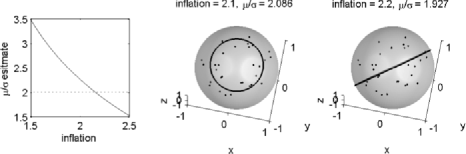
Figure 6: (Left) The estimate $\widehat{\mu/\sigma}$ decreases smoothly as the perturbation is inflated. (Center, right) Snapshots of the toy data on a sphere. A very small perturbation of the data set leads to a sharp transition between the small circle (center) and great circle (right).

4 Principal arc analysis on direct product manifolds

The discussions of the principal circles in $S^{2}$ play an important role in defining the principal arcs for data in a direct product manifold $M=M_{1}\,\otimes\,M_{2}\,\otimes\,\cdots\,\otimes\,M_{d}$, where each $M_{i}$ is one of the simple manifolds $S^{1}$, $S^{2}$, $\mathbb{R}_{+}$ and $\mathbb{R}$. We emphasize again that the curvature of the direct product manifold $M$ is mainly due to the spherical components.

Consider a data set $x_{1},\ldots,x_{n}\in M$, where $x_{i}\equiv(x_{i}^{1},\ldots,x_{i}^{d})$ such that $x_{i}^{j}\in M_{j}$. Denote $d_{0}\geq d$ for the intrinsic dimension of $M$. The geodesic mean $\bar{x}$ of the data is defined component-wise for each simple manifold $M_{j}$. Similarly, the tangent plane at $\bar{x}$, $T_{\bar{x}}M$, is also defined marginally, that is, $T_{\bar{x}}M$ is a direct product of tangent spaces of the simple manifolds. This tangent space gives a way of applying Euclidean space-based statistical methods by mapping the data onto $T_{\bar{x}}M$. We can manipulate this approximation of the data component-wise. In particular, the marginal data on the $S^{2}$ components can be represented in a linear space by a transformation $h_{\bar{\delta}}$, depending on the principal circles, that differs from the tangent space approximation.

Since the principal circles $\bar{\delta}$ capture the nongeodesic directions of variation, we use the principal circles as axes, which can be thought of as flattening the quadratic form of variation. In principle, we require a mapping $h_{\bar{\delta}}\dvtx S^{2}\rightarrow\mathbb{R}^{2}$ to have the following properties: For $\bar{\delta}=(\delta_{1},\delta_{2})=((\delta_{1}(\mathbf{c},r),\mathbf{u})$:

• $\mathbf{u}$ is mapped to the origin,

• $\delta_{1}$ is mapped onto the $x$-axis, and

• $\delta_{2}$ is mapped onto the $y$-axis.

Two reasonable choices of the mapping $h_{\bar{\delta}}$ will be discussed in Section 4.1 in detail.

The mapping $h_{\bar{\delta}}$ and the tangent space projection together give a linear space representation of the data where the Euclidean PCA is applicable. The line segments corresponding to the sample principal component direction of the transformed data can be mapped back to $M$, and become the principal arcs.

A procedure for principal arc analysis is as follows:

1. [(2)]

2. For each $j$ such that $M_{j}$ is $S^{2}$, compute principal circles $\bar{\delta}=\bar{\delta}(x_{1}^{j},\ldots,x_{2}^{j})$ and the ratio $\widehat{\mu/\sigma}$. If the ratio is greater than the predetermined value $\varepsilon=2$, then $\bar{\delta}$ is adjusted to be great circles as explained in Section 2.

3. Let $\mathbf{h}\dvtx M\rightarrow\mathbb{R}^{d_{0}}$ be a transformation $\mathbf{h}(x)=(h_{1}(x^{1}),\ldots,h_{d}(x^{d}))$. Each component of $\mathbf{h}$ is defined as

   $$h_{j}(x^{j})=\cases{h_{\bar{\delta}}(x^{j})&\quad\mbox{for }$M_{j}={S^{2}}$,\cr\operatorname{Log}_{\bar{x}^{j}}(x^{j})&\quad\mbox{otherwise},}$$

   where $\operatorname{Log}_{\bar{x}^{j}}$ and $h_{\bar{\delta}}$ are defined in the Appendix and Section 4.1, respectively.

4. Observe that $\mathbf{h}(x_{1}),\ldots,\mathbf{h}(x_{n})\in\mathbb{R}^{d_{0}}$ always have their mean at the origin. Thus, the singular value decomposition of the $d_{0}\times n$ data matrix $\mathbf{X}\equiv[\mathbf{h}(x_{1})\cdots\mathbf{h}(x_{n})]$ can be used for computation of the PCA. Let $\mathbf{v}_{1},\mathbf{v}_{2},\ldots,\mathbf{v}_{m}$ be the left singular vectors of $\mathbf{X}$ corresponding to the largest $m$ singular values.

5. The $k$th principal arc is obtained by mapping the direction vectors $\mathbf{v}_{k}$ onto $M$ by the inverse of $h$, which can be computed component-wise.

The principal arcs on $M$ are not, in general, geodesics. Nor are they necessarily circles, in the original marginal $S^{2}$. This is because $h_{\bar{\delta}}$ and its inverse $h_{\bar{\delta}}^{-1}$ are nonlinear transformations and, thus, a line on $\mathbb{R}^{2}$ may not be mapped to a circle in $S^{2}$. This is consistent with the fact that the principal components on a subset of variables are different from projections of the principal components from the whole variables.

Principal arc analysis for data on direct product manifolds often results in a concise summary of the data. When we observe a significant variation along a small circle of a marginal $S^{2}$, that is most likely not a random artifact but, instead, the result of a signal driving the circular variation. Nongeodesic variation of this type is well captured by our method.

Principal arcs can be used to reduce the intrinsic dimensionality of $M$. Suppose we want to reduce the dimension by $k$, where $k$ can be chosen by inspection of the scree plot. Then each data point $x$ is projected to a $k$-dimensional submanifold $M_{0}$ of $M$ in such a way that

$$\mathbf{h}^{-1}\Biggl{(}\sum_{i=1}^{k}\mathbf{v}_{i}\mathbf{v}_{i}^{\prime}\mathbf{h}(x)\Biggr{)}\in M_{0},$$

where the $\mathbf{v}_{i}$’s are the principal direction vectors in $\mathbb{R}^{d_{0}}$, found by step 3 above. Moreover, the manifold $M_{0}$ can be parameterized by the $k$ principal components $z_{1},\ldots,z_{k}$ such that $M_{0}(z_{1},\ldots,z_{k})=\mathbf{h}^{-1}(\sum_{i=1}^{k}z_{i}\mathbf{v}_{i})$.

4.1 Choice of the transformation $h_{\bar{\delta}}$

The transformation $h_{\bar{\delta}}\dvtx S^{2}\rightarrow\mathbb{R}^{2}$ leads to an alternative representation of the data, which differs from the tangent space projection. The $h_{\bar{\delta}}$ transforms nongeodesic scatters along $\delta_{1}$ to scatters along the $x$-axis, which makes a linear method like the PCA applicable. Among many choices of transformations that satisfy the three principles we stated, two methods are discussed here. Recall that $\bar{\delta}=(\delta_{1},\delta_{2})=(\delta_{1}(\mathbf{c},r),\mathbf{u})$.

Projection. The first approach is based on the projection of $\mathbf{x}$ onto $\delta_{1}$, defined in (3), and a residual $\xi$. The signed distance from $\mathbf{u}$ to $P_{\delta_{1}}x$, whose unsigned version is defined in (4), becomes the $x$-coordinate, while the residual $\xi$ becomes the $y$-coordinate. This approach has the same spirit as the model for the circle class (5), since the direction of the signal is mapped to the $x$-axis, with the perpendicular axis for errors.

The projection $h_{\bar{\delta}}(\mathbf{x})$ that we define here is closely related to the spherical coordinate system. Assume $\mathbf{c}=\mathbf{e}_{3}$, and $\mathbf{u}$ is at the Prime meridian (i.e., on the $x-z$ plane). For $\mathbf{x}$ and its spherical coordinates $(\phi,\theta)$ such that $\mathbf{x}=(x_{1},x_{2},x_{3})=(\cos\phi\sin\theta,\cos\phi\sin\theta,\cos\theta)$,

$$h_{\bar{\delta}}(\mathbf{x})=\bigl{(}\sin(r)\phi,\theta-\theta_{\mathbf{u}}\bigr{)},$$ (9)

where $\theta_{\mathbf{u}}=\cos^{-1}(u_{3})$ is the latitude of $\mathbf{u}$. The set of $h_{\bar{\delta}}(\mathbf{x}_{i})$ has mean zero because the principal circle mean $\mathbf{u}$ has been subtracted.

Conformal map. A conformal map is a function which preserves angles. We point out two conformal maps that can be combined to serve our purpose. See Chapter 9 of Churchill and Brown (1984) and Krantz (1999) for detailed discussions of conformal maps. A conformal map is usually defined in terms of complex numbers. Denote the extended complex plane $\mathbb{C}\cup\{\infty\}$ as $\mathbb{C}^{*}$. Let $\phi_{\mathbf{c}}:S^{2}\rightarrow\mathbb{C}^{*}$ be the stereographic projection of the unit sphere when the point antipodal from $\mathbf{c}$ is the projection point. Then $\phi_{\mathbf{c}}$ is a bijective conformal mapping defined for all $S^{2}$ that maps $\delta_{1}$ as a circle centered at the origin in $\mathbb{C}^{*}$. The linear fractional transformation, sometimes called the Möbius transformation, is a rational function of complex numbers, that can be used to map a circle to a line in $\mathbb{C}^{*}$. In particular, we define a linear fractional transformation $f_{u^{*}}\dvtx\mathbb{C}^{*}\rightarrow\mathbb{C}^{*}$ as

$$f_{u^{*}}(z)=\cases{\displaystyle\frac{\alpha i(z-u^{*})}{-z-u^{*}}&\quad\mbox{if }$z\neq-u^{*}$,\cr\infty&\quad\mbox{if }$z=-u^{*}$,}$$ (10)

where $u^{*}=\phi_{\mathbf{c}}(\mathbf{u})$, and $\alpha$ is a constant scalar. Then the image of $\delta_{1}$ under $f_{u^{*}}\circ\phi_{c}$ is the real axis, while the image of $\delta_{2}$ is the imaginary axis. The mapping $h_{\bar{\delta}}\dvtx S^{2}\rightarrow\mathbb{R}^{2}$ is defined by $f_{u^{*}}\circ\phi_{c}$ with the resulting complex numbers understood as members of $\mathbb{R}^{2}$. Note that orthogonality of any two curves in $S^{2}$ is preserved by the $h_{\bar{\delta}}$ but the distances are not. Thus, we use the scale parameter $\alpha$ of the function $f_{u^{*}}$ to match the resulting total variance of $h_{\bar{\delta}}(\mathbf{x}_{i})$ to the geodesic variance of $\mathbf{x}_{i}$.

In many cases, both projection and conformal $h_{\bar{\delta}}$ give better representations than just using the tangent space. Figure 7 illustrates the image of $h_{\bar{\delta}}$ with the toy data set depicted in Figure 2c. The tangent space mapping is also plotted for comparison. The tangent space mapping leaves the curvy form of variation, while both $h_{\bar{\delta}}$’s capture the variation and lead to an elliptical distribution of the transformed data.

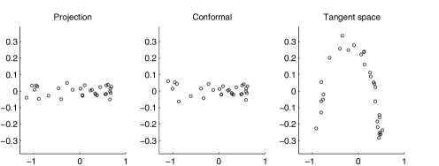
Figure 7: Illustration of projection $h_{\bar{\delta}}$ [left, equation (9)] and conformal $h_{\bar{\delta}}$ [center, equation (10)] compared to a tangent plane projection at the geodesic mean (right) of the data in Figure 2c. The $h_{\bar{\delta}}$ maps the variation along $\delta_{1}$ to the variation along the $x$-axis, while the tangent plane mapping fails to do so.

The choice between the projection and conformal mappings is a matter of philosophy. The image of the projection $h_{\bar{\delta}}$ is not all of $\mathbb{R}^{2}$, while the image of the conformal $h_{\bar{\delta}}$ is all of $\mathbb{R}^{2}$. However, in order to cover $\mathbb{R}^{2}$ completely, the conformal $h_{\bar{\delta}}$ can grossly distort the covariance structure of the data. In particular, the data points that are far from $\mathbf{u}$ are sometimes overly diffused when the conformal $h_{\bar{\delta}}$ is used, as can be seen in the left tail of the conformal mapped image in Figure 7. The projection $h_{\bar{\delta}}$ does not suffer from this problem. Moreover, the interpretation of projection $h_{\bar{\delta}}$ is closely related to the circle class model. Therefore, we recommend the projection $h_{\bar{\delta}}$, which is used in the following data analysis.

5 Application to m-rep data

In this section an application of Principal Arc Analysis to the medial representation (m-rep) data example, introduced below in more detail, is described.

5.1 Medial representation

The m-rep gives an efficient way of representing 2- or 3-dimensional objects. The m-rep is constructed from the medial axis, which is a means of representing the middle of geometric objects. The medial axis of a 3-dimensional object is formed by the centers of all spheres that are interior to objects and tangent to the object boundary at two or more points. In addition, the medial description is defined by the centers of the inscribed spheres and by the associated vectors, called spokes, from the sphere center to the two respective tangent points on the object boundary. The medial axis is sampled over an approximately regular lattice and the elements of the lattice are called medial atoms. A medial atom consists of the location of the atom combined with two equal-length spokes, defined as a 4-tuple:

• location in $\mathbb{R}^{3}$;

• spoke direction 1, in $S^{2}$;

• spoke direction 2, in $S^{2}$;

• common spoke length in $\mathbb{R}_{+}$;

as shown in Figure 8. The size of the regular lattice is fixed for each object in practice. For example, the shape of a prostate is usually described by a $3\times 5$ grid of medial atoms, across all samples. The collection of the medial atoms is called the medial representation (m-rep). An m-rep corresponds to a particular shape of prostate, and is a point in the m-rep space $\mathcal{M}$. The space of prostate m-reps is then $\mathcal{M}=(\mathbb{R}^{3}\otimes\mathbb{R}_{+}\otimes S^{2}\otimes S^{2})^{15}$, which is a 120-dimensional direct product manifold with $60$ components. The m-rep model provides a useful framework for describing shape variability in intuitive terms. See Siddiqi and Pizer (2008) and Pizer et al. (2003) for detailed introduction to and discussion of this subject.

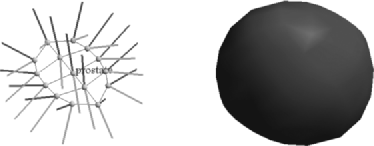
Figure 8: (Left) An m-rep model with $3\times 5$ grids of medial atoms. Each atom has its location ($\mathbb{R}^{3}$) and two equal-length spokes ($\mathbb{R}_{+}\otimes S^{2}\otimes S^{2}$). (Right) The implied surface of the m-rep model, showing a prostate shape.

An important topic in medical imaging is developing segmentation methods of 3D objects from CT images; see Cootes and Taylor (2001) and Pizer et al. (2007). A popular approach is similar to a Bayesian estimation scheme, where the knowledge of anatomic geometries is used (as a prior) together with a measure of how the segmentation matches the image (as a likelihood). A prior probability distribution is modeled using m-reps as a means of measuring geometric atypicality of a segmented object. PCA-like methods (including PAA) can be used to reduce the dimensionality of such a model. A detailed description can be found in Pizer et al. (2007).

5.2 Simulated m-rep object

The data set partly plotted in Figure 1 is from the generator discussed in Jeong et al. (2008). It generates random samples of objects whose shape changes and motions are physically modeled (with some randomness) by anatomical knowledge of the bladder, prostate and rectum in the male pelvis. Jeong et al. have proposed and used the generator to estimate the probability distribution model of shapes of human organs.

In the data set of 60 samples of prostate m-reps we studied, the major motion of prostate is a rotation. In some $S^{2}$ components, the variation corresponding to the rotation is along a small circle. Therefore, PAA should fit better for this type of data than principal geodesics. To make this advantage more clear, we also show results from a data set by removing the location and the spoke length information from the m-reps, the sample space of which is then $\{S^{2}\}^{30}$.

We have applied PAA as described in the previous section. The ratios $\mu/\sigma$, estimated for the 30 $S^{2}$ components, are in general large (with minimum 21.2, median 44.1 and maximum 118), which suggests use of small circles to capture the variation.

Figure 9 shows the proportion of the cumulative variances, as a function of number of components, from the Principal Geodesic Analysis (PGA) of Fletcher et al. (2004) and PAA. In both cases, the first principal arc leaves smaller residuals than the first principal geodesic. What is more important is illustrated in the scatterplots of the data projected onto the first two principal components. The quadratic form of variation that requires two PGA components is captured by a single PAA component.

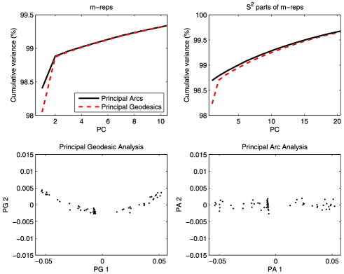
Figure 9: (Top) The proportion of variances captured by the first few components of PAA are compared to those from PGA for the simulated prostate m-reps. (Bottom) Scatter plots of the data on $\{S^{2}\}^{30}$ show that the major variation is explained more concisely by the first principal arc.

The probability distribution model estimated by principal geodesics is qualitatively different from the distribution estimated by PAA. Although the difference in the proportion of variance captured is small, the resulting distribution from PAA is no longer elliptical. In this sense, PAA gives a convenient way to describe a nonelliptical distribution by, for example, a Normal density.

5.3 Prostate m-reps from real patients

We also have applied PAA to a prostate m-rep data set from real CT images. Our data consist of five patients’ image sets, each of which is a series of CT scans containing prostate taken during a series of radiotherapy treatments [Merck (2008)]. The prostate in each image is manually segmented by experts and an m-rep model is fitted. The patients, coded as 3106, 3107, 3109, 3112 and 3115, have different numbers of CT scans (17, 12, 18, 16 and 15, respectively). We have in total 78 m-reps.

The proportion of variation captured in the first principal arc is 40.89%, slightly higher than the 40.53% of the first principal geodesic. Also note that the estimated probability distribution model from PAA is different from that of PGA. In particular, PAA gives a better separation of patients in the first two components, as depicted in the scatter plots (Figure 10).

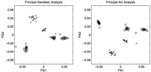
Figure 10: The scatter plots of the real prostate m-rep data. Different symbols represent different patients. PAA (right) gives a better separation of different patients in the first two components compared to PGA (left).

6 Doubly iterative algorithm to find the least-squares small circle

We propose an algorithm to fit the least-squares small circle (1), which is a constrained nonlinear minimization problem. This algorithm is best understood in two iterative steps: The outer loop approximates the sphere by a tangent space; the inner loop solves an optimization problem in the linear space, which is much easier than solving (1) directly. In more detail, the $(k+1)$th iteration works as follows. The sphere is approximated by a tangent plane at $\mathbf{c}_{k}$, the $k$th solution of the center of the small circle. For the points on the tangent plane, any iterative algorithm to find a least-squares circle can be applied as an inner loop. The solution of the inner iteration is mapped back to the sphere and becomes the $(k+1)$th input of the outer loop operation. One advantage of this algorithm lies in the reduced difficulty of the optimization task. The inner loop problem is much simpler than (1) and the outer loop is calculated by a closed-form equation, which leads to a stable and fast algorithm. Another advantage can be obtained by using the exponential map and log map (12) for the tangent projection, since they preserve the distance from the point of tangency to the others, that is, $\rho(\mathbf{x},\mathbf{c})=\|\operatorname{Log}_{\mathbf{c}}(\mathbf{x})\|$ for any $\mathbf{x}\in S^{2}$. This is also true for radii of circles. The exponential map transforms a circle in $\mathbb{R}^{2}$ centered at the origin with radius $r$ to $\delta(\mathbf{c},r)$. Thus, whenever (1) reaches its minimum, the algorithm does not alter the solution.

We first illustrate necessary building blocks of the algorithm. A tangent plane $T_{\mathbf{c}}$ at $\mathbf{c}$ can be defined for any $\mathbf{c}$ in $S^{2}$, and an appropriate coordinate system of $T_{\mathbf{c}}$ is obtained as follows. Basically, any two orthogonal complements of the direction $\mathbf{c}$ can be used as coordinates of $T_{\mathbf{c}}$. For example, when $\mathbf{c}=(0,0,1)^{\prime}\equiv\mathbf{e}_{3}$, a coordinate system is given by $\mathbf{e}_{1}$ and $\mathbf{e}_{2}$. For a general $\mathbf{c}$, let $q_{\mathbf{c}}$ be a rotation operator on $\mathbb{R}^{3}$ that maps $\mathbf{c}$ to $\mathbf{e}_{3}$. Then a coordinate system for $T_{\mathbf{c}}$ is given by the inverse of $q_{\mathbf{c}}$ applied to $\mathbf{e}_{1}$ and $\mathbf{e}_{2}$, which is equivalent to applying $q_{\mathbf{c}}$ to each point of $S^{2}$ and using $\mathbf{e}_{1}$, $\mathbf{e}_{2}$ as coordinates.

The rotation operator $q_{\mathbf{c}}$ can be represented by a rotation matrix. For $\mathbf{c}=(c_{x},c_{y},c_{z})^{\prime}$, the rotation $q_{\mathbf{c}}$ is equivalent to rotation through the angle $\theta=\cos^{-1}(c_{z})$ about the axis $\mathbf{u}=(c_{y},-c_{x},0)^{\prime}/\sqrt{1-c_{z}^{2}}$, whenever $\mathbf{c}\neq\pm\mathbf{e}_{3}$. When $\mathbf{c}=\pm\mathbf{e}_{3}$, $\mathbf{u}$ is set to be $\mathbf{e}_{1}$. It is well known that a rotation matrix with axis $\mathbf{u}=(u_{x},u_{y},u_{z})^{\prime}$ and angle $\theta$ in radians is, for $c=\cos(\theta)$, $s=\sin(\theta)$ and $v=1-\cos(\theta)$,

$$R_{\mathbf{c}}=\pmatrix{c+u_{x}^{2}v&u_{x}u_{y}v-u_{z}s&u_{x}u_{z}v+u_{y}s\cr u_{x}u_{y}v+u_{z}s&c+u_{y}^{2}v&u_{y}u_{z}v-u_{x}s\cr u_{x}u_{z}v-u_{y}s&u_{y}u_{z}v+u_{x}s&c+u_{z}^{2}v},$$ (11)

so that $q_{\mathbf{c}}(\mathbf{x})=R_{\mathbf{c}}\mathbf{x}$, for $\mathbf{x}\in\mathbb{R}^{3}$.

With the coordinate system for $T_{\mathbf{c}}$, we shall define the exponential map $\operatorname{Exp}_{\mathbf{c}}$, a mapping from $T_{\mathbf{c}}$ to $S^{2}$, and the log map $\operatorname{Log}_{\mathbf{c}}=\operatorname{Exp}_{\mathbf{c}}^{-1}$. These are defined for $\mathbf{v}=(v_{1},v_{2})\in\mathbb{R}^{2}$ and $\mathbf{x}=(x_{1},x_{2},x_{3})^{\prime}\in S^{2}$, as

$$\operatorname{Exp}_{\mathbf{c}}(\mathbf{v})=q_{\mathbf{c}}\circ\operatorname{Exp}_{\mathbf{e}_{3}}(\mathbf{v}),\qquad\operatorname{Log}_{\mathbf{c}}(\mathbf{x})=\operatorname{Log}_{\mathbf{e}_{3}}\circ\,q_{\mathbf{c}}(\mathbf{x}),$$ (12)

for $\theta=\cos^{-1}(x_{3})$. See (18)–(19) in the Appendix for $\operatorname{Exp}_{\mathbf{e}_{3}}$ and $\operatorname{Log}_{\mathbf{e}_{3}}$. Note that $\operatorname{Log}_{\mathbf{c}}(\mathbf{c})=\mathbf{0}$ and $\operatorname{Log}_{\mathbf{c}}$ is not defined for the antipodal point of $\mathbf{c}$.

Once we have approximated each $\mathbf{x}_{i}$ by $\operatorname{Log}_{\mathbf{c}}(\mathbf{x}_{i})\equiv\tilde{\mathbf{x}}_{i}$, the inner loop finds the minimizer $(\mathbf{v},r)$ of

$$\min\sum_{i=1}^{n}(\|\tilde{\mathbf{x}}_{i}-\mathbf{v}\|-r)^{2},$$ (13)

which is to find the least-squares circle centered at $\mathbf{v}$ with radius $r$. The general circle fitting problem is discussed in, for example, Umbach and Jones (2003) and Chernov (2010). This problem is much simpler than (1) because it is an unconstrained problem and the number of parameters to optimize is decreased by 1. Moreover, optimal solution of $r$ is easily found as

$$\hat{r}=\frac{1}{n}\sum_{i=1}^{n}\|\tilde{\mathbf{x}}_{i}-\mathbf{v}\|,$$ (14)

when $\mathbf{v}$ is given. Note that for great circle fitting, we can simply put $\hat{r}=\pi/2$. Although the problem is still nonlinear, one can use any optimization method that solves nonlinear least squares problems. We use the Levenberg–Marquardt algorithm, modified by Fletcher (1971) [see Chapter 4 of Scales (1985) and Chapter 3 of Bates and Watts (1988)], to minimize (13) with $r$ replaced by $\hat{r}$. One can always use $\mathbf{v}=\mathbf{0}$ as an initial guess since $\mathbf{0}=\operatorname{Log}_{\mathbf{c}}(\mathbf{c})$ is the solution from the previous (outer) iteration.

The algorithm is now summarized as follows:

1. [(1)]

2. Given $\{\mathbf{x}_{1},\ldots,\mathbf{x}_{n}\}$, $\mathbf{c}_{0}=\mathbf{x}_{1}$.

3. Given $\mathbf{c}_{k}$, find a minimizer $\mathbf{v}$ of (13) with $r$ replaced by (14), with inputs $\tilde{\mathbf{x}}_{i}=\operatorname{Log}_{\mathbf{c}_{k}}(\mathbf{x}_{i})$.

4. If $\|\mathbf{v}\|<\varepsilon$, then iteration stops with the solution $\hat{\mathbf{c}}=\mathbf{c}_{k}$, $r=\hat{r}$ as in (14). Otherwise, $\mathbf{c}_{k+1}=\operatorname{Exp}_{\mathbf{c}_{k}}(\mathbf{v})$ and go to step 2.

Note that the radius of the fitted circle in $T_{\mathbf{c}}$ is the same as the radius of the resulting small circle. There could be many variations of this algorithm: as an instance, one can elaborate the initial value selection by using the eigenvector of the sample covariance matrix of $\mathbf{x}_{i}$’s, corresponding to the smallest eigenvalue as done in Gray, Geiser and Geiser (1980). Experience has shown that the proposed algorithm is stable and speedy enough. Gray, Geiser and Geiser proposed to solve (1) directly, which seems to be unstable in some cases.

The idea of the doubly iterative algorithm can be applied to other optimization problems on manifolds. For example, the geodesic mean is also a solution of a nonlinear minimization, where the nonlinearity comes from the use of the geodesic distance. This can be easily solved by an iterative approximation of the manifold to a linear space [See Chapter 4 of Fletcher (2004)], which is the same as the gradient descent algorithms [Pennec (2006), Le (2001)]. Note that the proposed algorithm, like other iterative algorithms, only finds one solution even if there are multiple solutions.

Appendix: Some background on direct product manifold

We give some necessary geometric background on direct product manifolds. Precise definitions and geometric discussions on a richer class of manifold, Riemannian manifold, can be found in Boothby (1986) and Helgason (2001).

A $d$-dimensional manifold can be thought of as a curved surface embedded in a Euclidean space of higher dimension $d^{\prime}$ (${\geq}d$). The manifold is required to be smooth, that is, infinitely differentiable, so that a sufficiently small neighborhood of any point on the manifold can be well approximated by a linear space. The tangent space at a point $p$ of a manifold $M$, $T_{p}M$, is defined as a linear space of dimension $d$ which is tangent to $M$ at $p$. The notion of distance on $M$ is handled by a Riemannian metric, which is a metric of tangent spaces. In particular, the geodesic distance function $\rho_{M}(p,q)$ is roughly defined as the length of the shortest curve joining $p,q\in M$.

Now consider a direct product manifold $M=M_{1}\otimes\cdots\otimes M_{m}$. We restrict our attention to the case where each $M_{i}$ is one of the simple manifolds $S^{1},S^{2},\mathbb{R}_{+}$ or $\mathbb{R}$, but most of the assertions below apply equally well to direct products of more general manifolds.

Geodesic distance function. The geodesic distance between $p\equiv(p^{1},\ldots,p^{m})$ and $q\equiv(q^{1},\ldots,q^{m})$ is defined by

$$\rho_{M}(p,q)=\Biggl{(}\sum_{i=1}^{m}\rho_{M_{i}}^{2}(p^{i},q^{i})\Biggr{)}^{1/2},$$

where each $\rho_{M_{i}}$ is the geodesic distance function on $M_{i}$. The geodesic distance on $S^{1}$ is defined by the length of the shortest arc. Similarly, the geodesic distance on $S^{2}$ is defined by the length of the shortest great circle segment. The geodesic distance on $\mathbb{R}_{+}$ needs special treatment. In many practical applications, $\mathbb{R}_{+}$ represents a space of scale parameters. A desirable property for a metric on scale parameters is scale invariance, $\rho(rx,ry)=\rho(x,y)$ for any $x,y,r\in\mathbb{R}_{+}$. This can be achieved by differencing the logs, that is,

$$\rho_{\mathbb{R}_{+}}(x,y)=\bigg{|}\log\frac{x}{y}\bigg{|}\qquad\mbox{for }x,y\in\mathbb{R}_{+}.$$ (15)

Finally, the geodesic distance on a simple manifold $\mathbb{R}$ or $\mathbb{R}^{d}$ is the Euclidean distance.

Geodesic mean and variance. The geodesic mean of a set of points in $M$, also referred to as the intrinsic mean, is also calculated component-wise. The geodesic mean of $x_{1},\ldots,x_{n}\in M$ is the minimizer in $M$ of the sum of squared geodesic distances to the data. Thus, the geodesic mean is defined as

$$\bar{x}=\mathop{\mathrm{argmin}}_{x\in M}\frac{1}{n}\sum_{i=1}^{n}\rho_{M}^{2}(x,x_{i}).$$ (16)

In fact, each $\bar{x}^{i}$ of $\bar{x}=(\bar{x}^{1},\ldots,\bar{x}^{m})$ is the geodesic mean of $x_{1}^{i},\ldots,x_{n}^{i}\in M_{i}$. The geodesic mean of $\theta_{1},\ldots,\theta_{n}\in[0,2\pi)\cong S^{1}$ is found by examining a candidate set consisting of

$$\bar{\theta}_{j}=\frac{\sum_{i=1}^{n}\theta_{i}+2j\pi}{n},\qquad j=0,\ldots,n-1,$$ (17)

as in Moakher (2002). The geodesic mean in $S^{2}$ can be calculated by a full grid search or an iterative algorithm, as described in Section 6. The geodesic mean in $\mathbb{R}_{+}$ or $\mathbb{R}$ is straightforward. Note that the geodesic mean may not be unique. However, throughout the paper, we have assumed that the data have a unique geodesic mean which is true in most data analytic situations. Statistical investigation of the geodesic mean on manifolds can be found, for example, in Bhattacharya and Patrangenaru (2003, 2005) and Le and Kume (2000).

A related notion is geodesic variance. A sample geodesic variance is defined by the average squared geodesic distances to the geodesic mean, that is, $\frac{1}{n}\sum_{i=1}^{n}\rho^{2}_{M}(\bar{x},x_{i})$. When $M$ is indeed the Euclidean space, the geodesic variance is the same as the total variance (the trace of the variance–covariance matrix).

Mappings to tangent space. The exponential map maps a point in $T_{p}M$ to $M$. The log map is the inverse exponential map whose domain is in $M$. For a direct product manifold $M$, the mappings are also defined component-wise. For $S^{1}$, let $\theta\in\mathbb{R}$ denote an element of $T_{\mathbf{p}}S^{1}$ where $\mathbf{p}$ is set to be $(1,0)\in S^{1}$ embedded in $\mathbb{R}^{2}$. Then the exponential map is defined as

$$\operatorname{Exp}_{\mathbf{p}}(\theta)=(\cos\theta,\sin\theta).$$

The corresponding log map of $\mathbf{x}=(x_{1},x_{2})$ is defined as $\operatorname{Log}_{\mathbf{p}}(x)=\operatorname{sign}(x_{2})\cdot\mathop{\mathrm{arccos}}(x_{1})$. For $S^{2}$, let $\mathbf{v}=(v_{1},v_{2})$ denote a tangent vector in $T_{\mathbf{p}}S^{2}$. Let $\mathbf{p}=\mathbf{e}_{3}$, then the exponential map $\operatorname{Exp}_{\mathbf{p}}\dvtx T_{\mathbf{p}}S^{2}\longrightarrow S^{2}$ is defined by

$$\operatorname{Exp}_{\mathbf{p}}(\mathbf{v})=\biggl{(}\frac{v_{1}}{\|\mathbf{v}\|}\sin{\|\mathbf{v}\|},\frac{v_{2}}{\|\mathbf{v}\|}\sin{\|\mathbf{v}\|},\cos{\|\mathbf{v}\|}\biggr{)}.$$ (18)

This equation can be understood as a rotation of the base point $\mathbf{p}$ to the direction of $\mathbf{v}$ with angle $\|\mathbf{v}\|$. The corresponding log map for a point $\mathbf{x}=(x_{1},x_{2},x_{3})\in S^{2}$ is given by

$$\operatorname{Log}_{\mathbf{p}}(x)=\biggl{(}x_{1}\frac{\theta}{\sin{\theta}},x_{2}\frac{\theta}{\sin{\theta}}\biggr{)},$$ (19)

where $\theta=\mathop{\mathrm{arccos}}(x_{3})$ is the geodesic distance from $\mathbf{p}$ to $x$. Note that the antipodal point of $p$ is not in the domain of the log map, that is, the domain of $\operatorname{Log}_{\mathbf{p}}$ is $S^{2}/\{-\mathbf{p}\}$. In both $S^{1}$ and $S^{2}$, $\mathbf{p}$ can be set to be any point on $S^{1}$ or $S^{2}$. The exponential and log map for an arbitrary $T_{\mathbf{p}}$ can be defined together with a rotation operator, which is defined in Section 6 for the case of $S^{2}$. The exponential map of $\mathbb{R}_{+}$ is defined by the standard real exponential function. The domain of the inverse exponential map, the log map, is $\mathbb{R}_{+}$ itself. Finally, the exponential map on $\mathbb{R}$ is the identity map.

References

- Bates and Watts (1988) {bbook}[author] \bauthor\bsnmBates, \bfnmDouglas M.\binitsD. M. and \bauthor\bsnmWatts, \bfnmDonald G.\binitsD. G. (\byear1988). \btitleNonlinear Regression Analysis and Its Applications. \bseriesWiley Series in Probability and Mathematical Statistics: Applied Probability and Statistics. \bpublisherWiley, \baddressNew York. \MR1060528 \endbibitem
- Bhattacharya and Patrangenaru (2003) {barticle}[author] \bauthor\bsnmBhattacharya, \bfnmRabi\binitsR. and \bauthor\bsnmPatrangenaru, \bfnmVic\binitsV. (\byear2003). \btitleLarge sample theory of intrinsic and extrinsic sample means on manifolds. I. \bjournalAnn. Statist. \bvolume31 \bpages1–29. \MR1962498 \endbibitem
- Bhattacharya and Patrangenaru (2005) {barticle}[author] \bauthor\bsnmBhattacharya, \bfnmRabi\binitsR. and \bauthor\bsnmPatrangenaru, \bfnmVic\binitsV. (\byear2005). \btitleLarge sample theory of intrinsic and extrinsic sample means on manifolds. II. \bjournalAnn. Statist. \bvolume33 \bpages1225–1259. \MR2195634 \endbibitem
- Bingham and Mardia (1978) {barticle}[author] \bauthor\bsnmBingham, \bfnmChristopher\binitsC. and \bauthor\bsnmMardia, \bfnmK. V.\binitsK. V. (\byear1978). \btitleA small circle distribution on the sphere. \bjournalBiometrika \bvolume65 \bpages379–389. \MR0513936 \endbibitem
- Boothby (1986) {bbook}[author] \bauthor\bsnmBoothby, \bfnmW. M.\binitsW. M. (\byear1986). \btitleAn Introduction to Differentiable Manifolds and Riemannian Geometry, \bedition2nd ed. \bpublisherAcademic Press, Orlando, FL. \MR0861409 \endbibitem
- Chernov (2010) {bbook}[vtex] \bauthor\bsnmChernov, \bfnmNikolai\binitsN. (\byear2010). \btitleCircular and Linear Regression: Fitting Circles and Lines by Least Squares. \bpublisherChapman & Hall/CRC Press, \baddressBoca Raton, FL. \endbibitem
- Churchill and Brown (1984) {bbook}[author] \bauthor\bsnmChurchill, \bfnmRuel V.\binitsR. V. and \bauthor\bsnmBrown, \bfnmJames Ward\binitsJ. W. (\byear1984). \btitleComplex Variables and Applications, \bedition4th ed. \bpublisherMcGraw-Hill, \baddressNew York. \MR0730937 \endbibitem
- Cootes and Taylor (2001) {binproceedings}[vtex] \bauthor\bsnmCootes, \bfnmT. F.\binitsT. F. and \bauthor\bsnmTaylor, \bfnmC. J.\binitsC. J. (\byear2001). \btitleStatistical models of appearance for medical image analysis and computer vision. In \bbooktitleMedical Imaging 2001: Image Processing (\beditor\bfnmMilan\binitsM. \bsnmSonka and \beditor\bfnmKenneth M.\binitsK. M. \bsnmHanson, eds.). \bseriesProceedings of the SPIE \bvolume4322 \bpages236–248. \bpublisherSPIE. \endbibitem
- Cox (1969) {bincollection}[author] \bauthor\bsnmCox, \bfnmD. R.\binitsD. R. (\byear1969). \btitleSome sampling problems in technology. In \bbooktitleNew Developments in Survey Sampling (\beditor\bfnmU. L.\binitsU. L. \bsnmJohnson and \beditor\bfnmH.\binitsH. \bsnmSmith, eds.). \bpublisherWiley, New York. \endbibitem
- Elandt (1961) {barticle}[author] \bauthor\bsnmElandt, \bfnmRegina C.\binitsR. C. (\byear1961). \btitleThe folded normal distribution: Two methods of estimating parameters from moments. \bjournalTechnometrics \bvolume3 \bpages551–562. \MR0130738 \endbibitem
- Fisher (1993) {bbook}[author] \bauthor\bsnmFisher, \bfnmN. I.\binitsN. I. (\byear1993). \btitleStatistical Analysis of Circular Data. \bpublisherCambridge Univ. Press, \baddressCambridge. \MR1251957 \endbibitem
- Fisher, Lewis and Embleton (1993) {bbook}[author] \bauthor\bsnmFisher, \bfnmN. I.\binitsN. I., \bauthor\bsnmLewis, \bfnmT.\binitsT. and \bauthor\bsnmEmbleton, \bfnmB. J. J.\binitsB. J. J. (\byear1993). \btitleStatistical Analysis of Spherical Data. \bpublisherCambridge Univ. Press, \baddressCambridge. \MR1247695 \endbibitem
- Fletcher (1971) {btechreport}[author] \bauthor\bsnmFletcher, \bfnmR\binitsR. (\byear1971). \btitleA modified Marquardt subroutine for non-linear least squares. \btypeTechnical Report \bnumberAERE-R 6799. \endbibitem
- Fletcher (2004) {bphdthesis}[author] \bauthor\bsnmFletcher, \bfnmP. Thomas\binitsP. T. (\byear2004). \btitleStatistical variability in nonlinear spaces: Application to shape analysis and DT-MRI. \btypePhD thesis, \bschoolUniv. North Carolina at Chapel Hill. \endbibitem
- Fletcher et al. (2004) {barticle}[author] \bauthor\bsnmFletcher, \bfnmP. Thomas\binitsP. T., \bauthor\bsnmLu, \bfnmConglin\binitsC., \bauthor\bsnmPizer, \bfnmStephen M.\binitsS. M. and \bauthor\bsnmJoshi, \bfnmSarang\binitsS. (\byear2004). \btitlePrincipal geodesic analysis for the study of nonlinear statistics of shape. \bjournalIEEE Trans. Med. Imaging \bvolume23 \bpages995–1005. \endbibitem
- Gray, Geiser and Geiser (1980) {barticle}[author] \bauthor\bsnmGray, \bfnmNorman H.\binitsN. H., \bauthor\bsnmGeiser, \bfnmPeter A.\binitsP. A. and \bauthor\bsnmGeiser, \bfnmJames R.\binitsJ. R. (\byear1980). \btitleOn the least-squares fit of small and great circles to spherically projected orientation data. \bjournalMath. Geol. \bvolume12 \bpages173–184. \MR0593408 \endbibitem
- Hastie and Stuetzle (1989) {barticle}[author] \bauthor\bsnmHastie, \bfnmTrevor\binitsT. and \bauthor\bsnmStuetzle, \bfnmWerner\binitsW. (\byear1989). \btitlePrincipal curves. \bjournalJ. Amer. Statist. Assoc. \bvolume84 \bpages502–516. \MR1010339 \endbibitem
- Helgason (2001) {bbook}[author] \bauthor\bsnmHelgason, \bfnmSigurdur\binitsS. (\byear2001). \btitleDifferential Geometry, Lie Groups, and Symmetric Spaces. \bseriesGraduate Studies in Mathematics \bvolume34. \bpublisherAmer. Math. Soc., Providene, RI. \MR1834454 \endbibitem
- Huckemann, Hotz and Munk (2010) {barticle}[author] \bauthor\bsnmHuckemann, \bfnmStephan\binitsS., \bauthor\bsnmHotz, \bfnmThomas\binitsT. and \bauthor\bsnmMunk, \bfnmAxel\binitsA. (\byear2010). \btitleIntrinsic shape analysis: Geodesic PCA for Riemannian manifolds modulo isometric lie group actions. \bjournalStatist. Sinica \bvolume20 \bpages1–58. \MR2640651 \endbibitem
- Huckemann and Ziezold (2006) {barticle}[author] \bauthor\bsnmHuckemann, \bfnmStephan\binitsS. and \bauthor\bsnmZiezold, \bfnmHerbert\binitsH. (\byear2006). \btitlePrincipal component analysis for Riemannian manifolds, with an application to triangular shape spaces. \bjournalAdv. in Appl. Probab. \bvolume38 \bpages299–319. \MR2264946 \endbibitem
- Jeong et al. (2008) {binproceedings}[vtex] \bauthor\bsnmJeong, \bfnmJa-Yeon\binitsJ.-Y., \bauthor\bsnmStough, \bfnmJoshua V.\binitsJ. V., \bauthor\bsnmMarron, \bfnmJ. S.\binitsJ. S. and \bauthor\bsnmPizer, \bfnmStephen M.\binitsS. M. (\byear2008). \btitleConditional-mean initialization using neighboring objects in deformable model segmentation. \bmiscIn \bbooktitleMedical Imaging 2008: Image Processing (\beditor\bfnmJoseph M.\binitsJ. M. \bsnmReinhardt and \beditor\bfnmJosien P. W.\binitsJ. P. W. \bsnmPluim, eds.). \bseriesProceedings of the SPIE \bvolume6914 \bpages69144R.1–69144R.9. \bpublisherSPIE. \endbibitem
- Johnson (1962) {barticle}[author] \bauthor\bsnmJohnson, \bfnmN. L.\binitsN. L. (\byear1962). \btitleThe folded normal distribution: Accuracy of estimation by maximum likelihood. \bjournalTechnometrics \bvolume4 \bpages249–256. \MR0137221 \endbibitem
- Karcher (1977) {barticle}[author] \bauthor\bsnmKarcher, \bfnmH.\binitsH. (\byear1977). \btitleRiemannian center of mass and mollifier smoothing. \bjournalComm. Pure Appl. Math. \bvolume30 \bpages509–541. \MR0442975 \endbibitem
- Krantz (1999) {bbook}[author] \bauthor\bsnmKrantz, \bfnmSteven G.\binitsS. G. (\byear1999). \btitleHandbook of Complex Variables. \bpublisherBirkhäuser, \baddressBoston, MA. \MR1738432 \endbibitem
- Le (2001) {barticle}[author] \bauthor\bsnmLe, \bfnmHuiling\binitsH. (\byear2001). \btitleLocating Fréchet means with application to shape spaces. \bjournalAdv. in Appl. Probab. \bvolume33 \bpages324–338. \MR1842295 \endbibitem
- Le and Kume (2000) {barticle}[author] \bauthor\bsnmLe, \bfnmHuiling\binitsH. and \bauthor\bsnmKume, \bfnmAlfred\binitsA. (\byear2000). \btitleThe Fréchet mean shape and the shape of the means. \bjournalAdv. in Appl. Probab. \bvolume32 \bpages101–113. \MR1765168 \endbibitem
- Leone, Nelson and Nottingham (1961) {barticle}[author] \bauthor\bsnmLeone, \bfnmF. C.\binitsF. C., \bauthor\bsnmNelson, \bfnmL. S.\binitsL. S. and \bauthor\bsnmNottingham, \bfnmR. B.\binitsR. B. (\byear1961). \btitleThe folded normal distribution. \bjournalTechnometrics \bvolume3 \bpages543–550. \MR0130737 \endbibitem
- Mardia and Gadsden (1977) {barticle}[author] \bauthor\bsnmMardia, \bfnmK. V.\binitsK. V. and \bauthor\bsnmGadsden, \bfnmR. J.\binitsR. J. (\byear1977). \btitleA circle of best fit for spherical data and areas of vulcanism. \bjournalJ. Roy. Statist. Soc. Ser. C \bvolume26 \bpages238–245. \endbibitem
- Mardia and Jupp (2000) {bbook}[author] \bauthor\bsnmMardia, \bfnmKanti V.\binitsK. V. and \bauthor\bsnmJupp, \bfnmPeter E.\binitsP. E. (\byear2000). \btitleDirectional Statistics. \bseriesWiley Series in Probability and Statistics. \bpublisherWiley, Chichester. \MR1828667 \endbibitem
- Merck (2008) {barticle}[author] \bauthor\bsnmMerck, \bfnmStephen M.\binitsS. M., \bauthor\bsnmTracton, \bfnmGregg\binitsG., \bauthor\bsnmSaboo, \bfnmRohit\binitsR., \bauthor\bsnmLevy, \bfnmJoshua\binitsJ., \bauthor\bsnmChaney, \bfnmEdward\binitsE., \bauthor\bsnmPizer, \bfnmStephen M.\binitsS. M. and \bauthor\bsnmJoshi, \bfnmSarang\binitsS. (\byear2008). \btitleTraining models of anatomic shape variability. \bjournalMed. Phys. \bvolume35 \bpages3584–3596. \endbibitem
- Moakher (2002) {barticle}[author] \bauthor\bsnmMoakher, \bfnmMaher\binitsM. (\byear2002). \btitleMeans and averaging in the group of rotations. \bjournalSIAM J. Matrix Anal. Appl. \bvolume24 \bpages1–16 (electronic). \MR1920548 \endbibitem
- Pennec (2006) {barticle}[vtex] \bauthor\bsnmPennec, \bfnmXavier\binitsX. (\byear2006). \btitleIntrinsic statistics on Riemannian manifolds: Basic tools for geometric measurements. \bjournalJ. Math. Imaging Vision \bvolume25 \bpages127–154. \endbibitem
- Pizer et al. (2003) {barticle}[author] \bauthor\bsnmPizer, \bfnmStephen M.\binitsS. M., \bauthor\bsnmFletcher, \bfnmP.T.\binitsP. T., \bauthor\bsnmFridman, \bfnmY.\binitsY., \bauthor\bsnmFritsch, \bfnmD.S.\binitsD. S., \bauthor\bsnmGash, \bfnmA. G.\binitsA. G., \bauthor\bsnmGlotzer, \bfnmJ. M.\binitsJ. M., \bauthor\bsnmJoshi, \bfnmS.\binitsS., \bauthor\bsnmThall, \bfnmA.\binitsA., \bauthor\bsnmTracton, \bfnmG.\binitsG., \bauthor\bsnmYushkevich, \bfnmP.\binitsP. and \bauthor\bsnmChaney, \bfnmE. L.\binitsE. L. (\byear2003). \btitleDeformable m-reps for 3D medical image segmentation. \bjournalInt. J. Comput. Vision \bvolume55 \bpages85–106. \endbibitem
- Pizer et al. (2007) {barticle}[author] \bauthor\bsnmPizer, \bfnmStephen M.\binitsS. M., \bauthor\bsnmBroadhurst, \bfnmRobert E.\binitsR. E., \bauthor\bsnmLevy, \bfnmJoshua\binitsJ., \bauthor\bsnmLiu, \bfnmXiaoxiao\binitsX., \bauthor\bsnmJeong, \bfnmJa-Yeon\binitsJ.-Y., \bauthor\bsnmStough, \bfnmJoshua\binitsJ., \bauthor\bsnmTracton, \bfnmGregg\binitsG. and \bauthor\bsnmChaney, \bfnmEdward L.\binitsE. L. (\byear2007). \btitleSegmentation by posterior optimization of m-reps: Strategy and results. Unpublished manuscript. \endbibitem
- Rivest (1999) {barticle}[author] \bauthor\bsnmRivest, \bfnmLouis-Paul\binitsL.-P. (\byear1999). \btitleSome linear model techniques for analyzing small-circle spherical data. \bjournalCanad. J. Statist. \bvolume27 \bpages623–638. \MR1745827 \endbibitem
- Scales (1985) {bbook}[author] \bauthor\bsnmScales, \bfnmL. E.\binitsL. E. (\byear1985). \btitleIntroduction to Nonlinear Optimization. \bpublisherSpringer, \baddressNew York. \MR0776609 \endbibitem
- Siddiqi and Pizer (2008) {bbook}[author] \bauthor\bsnmSiddiqi, \bfnmKaleem\binitsK. and \bauthor\bsnmPizer, \bfnmStephen\binitsS. (\byear2008). \btitleMedial Representations: Mathematics, Algorithms and Applications. \bpublisherSpringer, \baddressNew York. \MR2547467 \endbibitem
- Umbach and Jones (2003) {barticle}[author] \bauthor\bsnmUmbach, \bfnmDale\binitsD. and \bauthor\bsnmJones, \bfnmKerry N.\binitsK. N. (\byear2003). \btitleA few methods for fitting circles to data. \bjournalIEEE Transactions on Instrumentation and Measurement \bvolume52 \bpages1881–1885. \endbibitem