Orthogonal simple component analysis: A new, exploratory approach

Abstract

Combining principles with pragmatism, a new approach and accompanying algorithm are presented to a longstanding problem in applied statistics: the interpretation of principal components. Following Rousson and Gasser [53 (2004) 539–555]

the ultimate goal is not to propose a method that leads automatically to a unique solution, but rather to develop tools for assisting the user in his or her choice of an interpretable solution.

Accordingly, our approach is essentially exploratory. Calling a vector ‘simple’ if it has small integer elements, it poses the open question:

What sets of simply interpretable orthogonal axes—if any—are angle-close to the principal components of interest?

its answer being presented in summary form as an automated visual display of the solutions found, ordered in terms of overall measures of simplicity, accuracy and star quality, from which the user may choose. Here, ‘star quality’ refers to striking overall patterns in the sets of axes found, deserving to be especially drawn to the user’s attention precisely because they have emerged from the data, rather than being imposed on it by (implicitly) adopting a model. Indeed, other things being equal, explicit models can be checked by seeing if their fits occur in our exploratory analysis, as we illustrate. Requiring orthogonality, attractive visualization and dimension reduction features of principal component analysis are retained.

Exact implementation of this principled approach is shown to provide an exhaustive set of solutions, but is combinatorially hard. Pragmatically, we provide an efficient, approximate algorithm. Throughout, worked examples show how this new tool adds to the applied statistician’s armoury, effectively combining simplicity, retention of optimality and computational efficiency, while complementing existing methods. Examples are also given where simple structure in the population principal components is recovered using only information from the sample. Further developments are briefly indicated.

, and

1 Introduction and overview

Principal components are linear combinations of a set of, say, $p$ commensurable variables with coefficients (‘loadings’) given by eigenvectors of their covariance or correlation matrix $\mathbf{S}$. As such, they simultaneously enjoy many optimal properties: see, for example, Jolliffe (2002), Chapters 2 and 3. However, to be useful in practice, such components often need interpretation in the context of the data studied. Unfortunately, optimality is no guarantee of interpretability. Accordingly, principal components may possess optimal theoretical properties, but be of limited practical interest. This motivates replacing them by components which are more interpretable by virtue of being ‘simpler’ in some sense, albeit at the expense of some degree of optimality.

We begin with a brief overview of existing approaches to this problem, further details being available in the references cited.

1.1 Existing approaches

In a broad sense, simplicity means the appearance of nice structures in the loadings matrix $\mathbf{Q=(q}_{1}|\cdots|\mathbf{q}_{k}\mathbf{)}$ which contains the $k\leq p$ eigenvectors of interest. Often, the scientist in charge of the study would like to see if there are clear-cut patterns reflected in $\mathbf{Q}$ which help him or her to better understand the meaning of the components $\mathbf{q}_{r}^{\top}\mathbf{x}$ $(r=1,\ldots,k)$ which it generates. Examples of nice structures include the presence of simple weighted averages, contrasts, groups of variables and sparseness. However defined, simplicity inevitably implies some loss of optimality and it is the scientist in charge of the study who needs to calibrate the trade-off between simplicity and optimality, as we further comment in Section 1.2.

The oldest approach to simplifying principal components is rotation, exploiting the fact that—as with principal component analysis itself—rotation of the $p$ original axes (one for each variable) defines new orthogonal coordinate axes on which the data can be displayed while total variance is preserved. This provides attractive visualization and dimension reduction features. In particular, there being no double counting of total variance, the user can identify and plot the data on just those axes making the largest or smallest contributions to it, depending on the focus of scientific interest—explaining variability or exploring potential scientific laws (near constant linear relations among the variables).

Only rotation methods are guaranteed to provide new axes which are orthogonal. Nonrotation methods in general lack the attractive features noted above, joint visualization of components being impeded by nonorthogonality of axes and dimension reduction by loss of the additive decomposition of total variance.

Overall, the rotation approach to simplification seeks more interpretable, orthogonal axes while retaining as much optimality as possible. See, for example, Chapter 11 of Jolliffe (2002), which provides an excellent overall review of simplification of principal components as of 2002. More recently, assuming normality, Park (2005) has proposed a penalized profile likelihood method, using varimax as the penalty function, which favors rotation of ill-defined components (those whose eigenvalues are close). However, in all these methods, the loadings involved are usually real numbers, which means that interpretation can still be difficult.

Another approach to simplification is to target sparsity. The presence of many zeroes in $\mathbf{Q}$ can be useful for interpretation, for example, when dealing with many variables. See, for example, D’Aspremont et al. (2007), Farcomeni (2009), Chipman and Gu (2005) and the references therein. One class of methods which targets sparseness is that based on the Least Absolute Shrinkage Selection Operator (LASSO). See, for example, the papers by Trendafilov and Jolliffe (2007), Zou, Hastie and Tibshirani (2006), Sjöstrand, Stegmann and Larsen (2006) and Jolliffe, Trendafilov and Uddin (2003). Although most of these methods lead to orthogonal simplified components, combined with the presence of exact zero loadings, the remaining loadings are still real numbers, again impeding interpretation.

Other approaches simplify by imposing specific structures on the original data matrix $\mathbf{X}$ and can be seen as constrained singular value decompositions. For example, the semidiscrete decomposition (SDD) approach of Kolda and O’Leary (1998) restricts the loadings to lie in $\{-1,0,1\}$. Again, the nonnegative matrix factorization (NMF) approach of Lee and Seung (1999) requires the original variables to be nonnegative, decomposing $\mathbf{X}$ into two nonnegative factor matrices. More recently, plaid models [see, for example, Lazzeroni and Owen (2002)] impose various block structures on $\mathbf{X}$ which are useful for interpretation in gene expression microarray data. However, this class of methods does not require orthogonality of the simplified components, with the potential loss of attractive features noted above.

A more explicitly modeling approach to simplification has recently been suggested in Rousson and Gasser (2004). Intrinsically restricted to principal component analysis of a correlation matrix, it assumes a particular pattern in the eigenstructure of that matrix in which groups and contrasts of variables are forced to appear. Although not always appropriate, it is when all variables are positively correlated, the first eigenvector being then a weighted average of the variables and, consequently, the remaining eigenvectors being basically contrasts. The loadings obtained are all proportional to integers, aiding interpretation. However, the components obtained need not be orthogonal, again with the potential drawbacks noted above.

The approaches in Hausman (1982), Sun (2006) and Vines (2000) are similar to the one presented here, in the sense that all three give orthogonal components with loading vectors proportional to integers. Hausman’s method only allows the loadings to take the values $-1$, $0$ or $1$ and so is not always able to find a complete set of orthogonal vectors. In contrast, Vines’ method produces loading vectors that are proportional to integers via a sequence of pairwise ‘simplicity-preserving’ transformations which ensure that orthogonality is maintained. However, although always proportional to integers, the size of the integers is not bounded and may at times be very large. A fuller discussion of the method, and its properties, can be found in Sun (2006).

1.2 Interpretability

With others, we note that interpretability is neither guaranteed nor amenable to precise mathematical formulation, this latter being evidenced by the variety both between and within methods reviewed above.

These remarks have two key methodological consequences. First, whereas simplification can help in the vital step of interpretation, we do not expect any method to lead to interpretable results in all cases. And second, rather than attempt to find a unique optimal simplification in any predefined sense—in particular, rather than attempt to completely automate the trade-off between simplicity and optimality—they provide motivation for adopting an essentially exploratory approach which systematically produces an ordered range of solutions, from which the user can choose one or more preferred solutions.

Factors that can guide this choice include the following: (a) the criteria on which a method is based, (b) subject matter considerations, particular to the context of the data set under analysis, and (c) suboptimality with respect to exact principal component analysis, including loss of explanatory power—or of focus on potential scientific laws—and correlation. Only principal component analysis itself can give orthogonal loadings and uncorrelated components, and so any other rotation method will always show some degree of correlation.

1.3 Overview of a new approach

Beginning with a synoptic account, we give here an overview of our new, exploratory approach. Requiring orthogonality, it is based on three primary criteria: simplicity, angle-accuracy and ‘star quality.’

1.3.1 A synoptic account

Retaining the attractive visualization and dimension reduction features noted above, the approach to be presented is based on rotation to axes which are ‘simple’ in the sense—adopted henceforth—that each is defined by small integer loadings. It combines principles with pragmatism, complementing those already available. Following Rousson and Gasser (2004),

the ultimate goal is not to propose a method that leads automatically to a unique solution, but rather to develop tools for assisting the user in his or her choice of an interpretable solution.

Accordingly, our approach is essentially exploratory, posing the open question:

What sets of simply interpretable orthogonal axes—if any—are angle-close to the principal components of interest?

its answer being presented in summary form as an automated visual display of the solutions found, ordered in terms of overall measures of simplicity, angle-accuracy and star quality, from which the user may choose.

Here, ‘star quality’ refers to striking overall patterns in the sets of axes found, deserving to be especially drawn to the user’s attention precisely because they have emerged from the data, rather than been imposed on it by (implicitly) adopting a model. Indeed, other things being equal, explicit models can be checked by seeing if their fits occur in our essentially exploratory analysis, as we illustrate.

Our approach treats the components of interest equally, reflecting equal scientific interest in them. Along with later worked examples, the one that follows illustrates the appropriateness of adopting this principle. Adaptations of our methodology to other scientific contexts—notably, to those where interest focuses exclusively on explaining variability—are noted in Section 4.

Again, our approach trades angle-accuracy off against simplicity, with a bias toward the latter. Its exact implementation provides an exhaustive set of solutions but can be prohibitively hard, the solution space having combinatorial complexity which grows with $p$, $k$ and $N^{\ast}$, the maximum size of integer allowed. However, the nature of our approach allows efficient exploration of this vast space without restriction to any of its particular subsets, such as those determined by modeling assumptions. Pragmatically, we are able to provide an efficient, approximate algorithm for this computationally challenging problem.

1.3.2 A worked example: Blood flow data

A worked example illustrates this new approach. Figure 1, whose construction and terms are described in Section 2, summarizes its results on the covariance matrix for four different measurements of an index of resistance to flow in blood vessels [see the paper by Thompson, Vines and Harrington (1999)]. Here, $p=k=4$ and, as throughout the paper, we take the maximum integer allowed ($N^{\ast}$) to be $9$, this corresponding to allowing only single digit representations.

Figure 1: A graphical summary of the solutions obtained for the blood data by our approach.

Three solutions are obtained and ordered as shown, none of them being dominant in terms of both simplicity and accuracy. The user is referred first to the one ‘two star’ solution found, $\hat{S}_{1}$, also obtained by Vines (2000) and by the undeflated form of Chipman and Gu (2005) [recall that Rousson and Gasser (2004) cannot be used for covariance matrices]. This two star solution is also the simplest one found in this case, details being shown in Table 1 along with the original principal components.

Table 1: Principal component loadings for the blood flow data $\mathbf{q}_{1},\ldots,\mathbf{q}_{4}$ and the corresponding simplified loading vectors $\hat{\mathbf{z}}_{1},\ldots,\hat{\mathbf{z}}_{4}$ for solution $\widehat{S}_{1}$

Variable	$\bolds{\mathbf{q}_{1}}$	$\bolds{\hat{\mathbf{z}}_{1}}$	$\bolds{\mathbf{q}_{2}}$	$\bolds{\hat{\mathbf{z}}_{2}}$	$\bolds{\mathbf{q}_{3}}$	$\bolds{\hat{\mathbf{z}}_{3}}$	$\bolds{\mathbf{q}_{4}}$	$\bolds{\hat{\mathbf{z}}_{4}}$
Right doppler	0.42	$1$	$-0.32$	$-$10,	$-0.58$	$-$10,	$-0.62$	$-$10,
Left doppler	0.43	$1$	$0.30$	1	$-0.55$	$-1$0,	$0.65$	1
Right CVI	0.55	$1$	$-0.65$	$-$10,	$0.43$	1	$0.30$	1
Left CVI	0.58	$1$	$0.63$	1	$0.42$	1	$-0.31$	$-$10,
Variance (%)	58.000	$\phantom{0}57.0$	$25.9$	23.8	$9.5$	10.5	$6.5$	08.6

The simplified loadings here have a very clear structure and are easier to understand than the continuous ones, so much so, in fact, that it looks like we have uncovered nature’s design: a main effect, plus three orthogonal contrasts. The simplified components being orthogonal, the total variance is retained, being redistributed among the components so as to enhance interpretability. In particular, there is just a little loss in the variance explained by the first two components, while the relatively small variability in the last two suggests possible underlying regularities.

The user is referred next to the other, here ‘one star,’ solutions, starting with the simpler one. Having the same sign pattern, just different weights, they have essentially the same overall interpretation as $\hat{S}_{1}$. Successively gaining accuracy at the cost of some simplicity, the simplified loading vectors and percentages of variance explainedfor $\hat{S}_{2}$ and $\hat{S}_{3}$ are given in Table 2.

=280pt $\bolds{\hat{\bolds{S}}_{2}}$ $\bolds{\hat{\bolds{S}}_{3}}$ Variable $\bolds{\hat{\mathbf{z}}_{1}}$ $\bolds{\hat{\mathbf{z}}_{2}}$ $\bolds{\hat{\mathbf{z}}_{3}}$ $\bolds{\hat{\mathbf{z}}_{4}}$ $\bolds{\hat{\mathbf{z}}_{1}}$ $\bolds{\hat{\mathbf{z}}_{2}}$ $\bolds{\hat{\mathbf{z}}_{3}}$ $\bolds{\hat{\mathbf{z}}_{4}}$ Right doppler 1 $-$10, $-$10, $-$2000 2 $-$10, $-$30, $-$20, Left doppler 1 1 $-$10, 20, 2 1 $-$30, 2 Right CVI 1 $-$20, 1 10, 3 $-$20, 2 1 Left CVI 1 2 1 $-$1000 3 2 2 $-$10, Variance (%) 57.0 ,25.9 ,10.5 6.5 57.9 ,25.9 0,9.7 0,6.5

Table 2: Integer representations of solutions $\hat{S}_{2}$ and $\hat{S}_{3}$ for the blood flow data

Overall, as this and later examples will show, we can obtain good approximations in the sense that only small integers are used, while retaining closeness to the original components and exact orthogonality. A distinctive feature of our exploratory approach is that the user is provided with an ordered set of alternative views of the same data, from which s/he may choose.

We move now to put some flesh on the bones of the synoptic account above, noting first that intrinsic interest lies in eigenaxes, not eigenvectors.

1.3.3 Eigenvectors, eigenaxes and their approximation

Recall that interest centers on a $p\times k$ loadings matrix $\mathbf{Q=(q}_{1}|\cdots|\mathbf{q}_{k}\mathbf{)}$ containing the eigenvectors of interest. Without loss, these are normalized to unit length ($\|\mathbf{q}_{r}\|=1,$ $r=1,\ldots,k$), $\lambda_{1}>\cdots>\lambda_{k}$ being the corresponding eigenvalues. The overall sign of each eigenvector is arbitrary. Rather, interest really centers on the ordered set of axes $\mathbf{\pm Q:=(\pm q}_{1}|\cdots|\mathbf{\pm q}_{k}\mathbf{)}$, where we identify any pair of nonzero opposed vectors $\mathbf{\pm q}$ with the axis (line through the origin or one-dimensional subspace) $\ell(\mathbf{q}):=\{c\mathbf{q\dvtx-\infty}<c<\mathbf{\infty}\}$ containing them.

The approach taken here treats the columns of $\mathbf{\pm Q}$ equally. It retains their orthogonality while replacing each eigenaxis $\alpha=\ell(\mathbf{q})$ by another one $\hat{\alpha}=\ell(\hat{\mathbf{z}})$, close to it in angle terms, which is ‘simple’ in the sense that it contains a nonzero vector $\hat{\mathbf{z}}$ with small integer elements. There is no loss in taking the highest common factor of the absolute values of the nonzero elements of $\hat{\mathbf{z}}$, denoted $\operatorname{hcf}(|\hat{\mathbf{z}}|)$, to be $1$. For, if not, we can divide each element of $\hat{\mathbf{z}}$ by it, without changing $\ell(\hat{\mathbf{z}})$.

Overall then, $\mathbf{\pm Q}$ is approximated by $\mathbf{\pm}\widehat{\mathbf{Z}}:=(\pm\hat{\mathbf{z}}_{1}|\cdots|\mathbf{\pm}\hat{\mathbf{z}}_{k}\mathbf{)}$ where $\widehat{\mathbf{Z}}:=(\hat{\mathbf{z}}_{1}|\cdots|\hat{\mathbf{z}}_{k}\mathbf{)}$ belongs to the set $\mathcal{Z}(p,k)$ of all $p\times k$ integer matrices with nonzero, pairwise orthogonal columns in each of which the absolute values of the nonzero elements are coprime, two members of this set being axis-equivalent if they differ, at most, in the overall signs of their columns.

1.3.4 Four maxims

Our approach is driven by four maxims, adopted for specific methodological reasons. Briefly, these are as follows.

(1) Integers aid interpretation. This maxim speaks for itself: we require linear combinations of variables defined by simple vectors since they are typically much easier to interpret than the principal components which they approximate. Again, exact zeroes and simple averages appear naturally.

Approximating an eigenaxis $\alpha=l(\mathbf{q})$ by a simple axis $\hat{\alpha}=l(\hat{\mathbf{z}})$ where $\operatorname{hcf}(|\hat{\mathbf{z}}|)=1$, we call $\hat{\mathbf{z}}$ an integer representation of $\hat{\alpha}$ and the maximum absolute value of its elements the complexity of $\hat{\mathbf{z}}$—interchangeably, of $\hat{\alpha}$—denoting these complexities by $\mathit{compl}(\hat{\mathbf{z}})\equiv\mathit{compl}(\hat{\alpha})$.

Other things being equal, we seek to keep the complexity of each $\hat{\alpha}_{r}$ $(r=1,\ldots,k)$ as low as possible.

(2) Be angle accurate (for the $k$ eigenvectors of interest). By keeping each approximating vector angle-close to its exact counterpart, we ensure that we do not lose potentially meaningful individual eigenvectors and that overall optimality is maximally retained. This is consistent with our principle of equal treatment of all the eigenaxes of interest, while providing a natural, operational measure of discrepancy, both for each axis separately and—it turns out—overall.

More specifically, we measure the discrepancy with which a simple axis $\hat{\alpha}=\mathbf{\pm}\hat{\mathbf{z}}$ approximates an eigenaxis $\alpha=\mathbf{\pm q}$ by the acute angle

$$d(\alpha,\hat{\alpha}):=\arccos\biggl{(}\frac{|\mathbf{q}^{\top}\hat{\mathbf{z}}|}{\|\mathbf{q}\|\|\hat{\mathbf{z}}\|}\biggr{)}$$ (1)

between them, this being a (geodesic) distance measure between axes. Equivalently, for reporting purposes, we may use the accuracy measure

$$\mathit{accu}(\alpha,\hat{\alpha}):=\cos(d(\alpha,\hat{\alpha})),$$

this taking values in $[0,1]$.

It turns out that, when approximating each of a set of axes, the greater the minimum angle-accuracy attained overall, the closer the original and approximating sets are in terms of a natural measure of distance (see Appendix A).

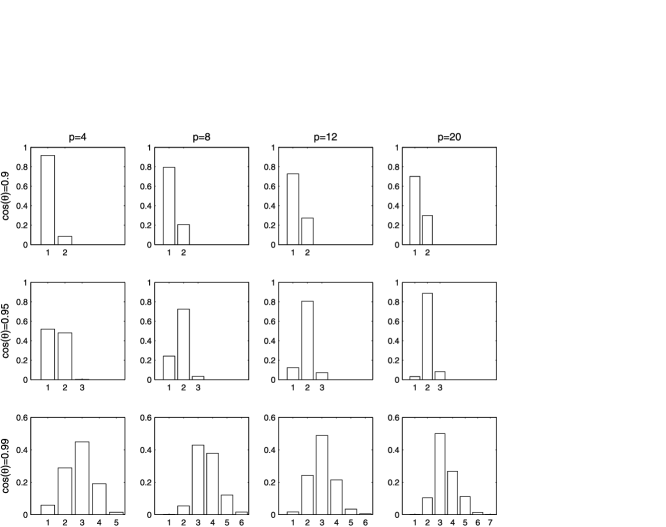
Figure 2: Empirical distribution of minimum complexities $N_{1}(\theta)$ in simple approximations to $p$-dimensional space.

(3) Be biased toward simplicity. It is always possible to approximate with reasonably high accuracy a single $p$-dimensional axis $\ell(\mathbf{q})$ by a simple axis of low complexity. Figure 2 shows, for different values of $p$ and $\cos(\theta)$, the empirical distribution (based on 10,000 independent replications) of the minimum complexity $N_{1}(\theta)$ required for there to be a simple axis having accuracy greater than $\cos(\theta)$ when $\ell(\mathbf{q})$ is sampled from the uniform distribution over the set of all possible axes [see Fang and Li (1997)]. Clearly, without orthogonality restrictions, accurate approximations of axes tend not to be very complex.

However, there is a clear trade-off between simplicity and accuracy: highly accurate approximations usually have high complexity, making interpretation more difficult. In general, we choose the simplest possible axis that is accurate enough, this bias toward simplicity being, in effect, a bias toward interpretability. In other words, in case of conflict, we favor maxim 1 over maxim 2.

(4) Orthogonality brings benefits. Primarily, we choose orthogonality because it aids interpretation. Our rotation approach enjoys the general visualization and dimension reduction features recalled above. Although none of these additional features is either targeted or imposed, sparsity, contrasts, simple relations between components and groups of variables may all emerge as a consequence of using orthogonality combined with integer coefficients. Orthogonality is also useful at several stages of the development, as we note.

1.4 Organization and running example

Section 2 develops these maxims into a methodology, the running example below being used for illustration throughout. The reader interested primarily in how this new approach performs may wish to skip this development and go straight to Section 2.5, where its results are summarized. Further examples are given in Section 3. Section 4 gives a short discussion of complements and extensions. Technical and computational details are given as Appendices.

=230pt $\bolds{\mathbf{q}_{1}}$ $\bolds{\mathbf{q}_{2}}$ $\bolds{\mathbf{q}_{3}}$ $\bolds{\mathbf{q}_{4}}$ $\bolds{\mathbf{q}_{5}}$ Mechanics (closed) 0.40 $-$0.65 $-$0.62 $-$0.15 $-$0.13 Vectors (closed) 0.43 $-$0.44 $-$0.71 $-$0.30 $-$0.18 Algebra (open) 0.50 $-$0.13 $-$0.04 $-$0.11 $-$0.85 Analysis (open) 0.46 $-$0.39 $-$0.14 $-$0.67 $-$0.42 Statistics (open) 0.40 $-$0.47 $-$0.31 $-$0.66 $-$0.23 Variance (%) 63.600 14.8, ,8.9 ,7.8 ,4.9

Table 3: Principal component loadings for the exams data

The running example used is based on Table 3 which shows the unit length eigenvectors (rounded to 2 decimal places) of the sample correlation matrix for a data set consisting of the scores achieved by $88$ students in $p=k=5$ tests, a combination of open- and closed-book exams [Mardia, Kent and Bibby (1979)]. Thus, the first principal component is a weighted average of all the different subject scores, while the other principal components can be interpreted as contrasts. However, more detailed interpretation of the principal components, particularly those other than the first, is not easy.

Throughout, $\mathbb{Z}^{p}$ denotes the set of all $p\times 1$ vectors with integer elements—positive, negative or zero—and $\mathbb{Z}^{(p)}$ the same set with the zero vector removed. Replacing integers by real numbers, the corresponding sets are denoted $\mathbb{R}^{p}$ and $\mathbb{R}^{(p)}$, respectively.

2 A new approach

2.1 A sequential approach

Operationally, we approximate the $k$ eigenaxes of interest sequentially. The order in which we do this matters, for two principal reasons: earlier approximations restrict the approximations available for later eigenaxes and, hence, their maximum possible achievable accuracy.

To illustrate these points consider, say, the ‘forwards’ $1$ to $k$ order from high to low eigenvalue. When dealing with $\alpha_{1}$, there are no orthogonality restrictions and we seek an approximation $\hat{\alpha}_{1}$ to it in the set $\mathcal{M}_{1}$ of all simple axes in $\mathbb{R}^{p}$. In contrast, for each $r\in\{2,\ldots,k\}$, we seek an approximation $\hat{\alpha}_{r}$ to $\alpha_{r}$ within the set $\mathcal{M}_{r}$ of all simple axes in $\mathbb{R}^{p}$ orthogonal to each of $\hat{\alpha}_{1},\ldots,\hat{\alpha}_{r-1}$.

Thus, for the exams data, $\mathcal{M}_{1}$ is the set of all axes generated by vectors in $\mathbb{Z}^{(5)}$ while, for example, taking $\hat{\mathbf{z}}_{1}=(1,1,1,1,1)^{\top}$, $\ell((1,1,0,-1,-1)^{\top})$ is a member of $\mathcal{M}_{2}$, but $\ell((1,1,0,0,-1)^{\top})$ is not.

The second point is clear geometrically. The angle-closest axis to $\alpha$ orthogonal to $\hat{\alpha}_{1},\ldots,\hat{\alpha}_{r-1}$ is its projection onto the orthogonal complement of their span. This restricts the maximum accuracy that can be achieved. For, if $\mathbf{q}_{r}^{\perp}$ is the orthogonal projection of the unit vector $\mathbf{q}_{r}$ onto the orthogonal complement of $\operatorname{Span}\{\mathbf{z}_{1},\ldots,\mathbf{z}_{r-1}\}$, some straightforward trigonometry shows that any approximation $\hat{\alpha}\in\mathcal{M}_{r}$ satisfies

$$\mathit{accu}(\alpha_{r},\hat{\alpha}) = \mathit{accu}(\alpha_{r},\ell(\mathbf{q}_{r}^{\bot}))\mathit{accu}(\ell(\mathbf{q}_{r}^{\bot}),\hat{\alpha})$$

$$= \|\mathbf{q}_{r}^{\perp}\|\mathit{accu}(\ell(\mathbf{q}_{r}^{\perp}),\hat{\alpha}),$$

so that $\mathit{accu}(\alpha_{r},\hat{\alpha})\leq\|\mathbf{q}_{r}^{\perp}\|$, equality holding if and only if $\hat{\alpha}=\ell(\mathbf{q}_{r}^{\perp})$[which requires $\ell(\mathbf{q}_{r}^{\perp})$ to be simple]. Thus, over $\mathcal{M}_{r}$, not every possible accuracy is achievable for $\alpha_{r}$ ($r>1$), although no such upper bound applies to $\mathit{accu}(\ell(\mathbf{q}_{r}^{\perp}),\hat{\alpha})$.

Table 4: Integer representations for the examinations data with $\theta=\pi/4$

Variable	$\bolds{\hat{\mathbf{z}}_{1}(\theta)}$	$\bolds{\hat{\mathbf{z}}_{2}(\theta)}$	$\bolds{\hat{\mathbf{z}}_{3}(\theta)}$	$\bolds{\hat{\mathbf{z}}_{4}(\theta)}$	$\bolds{\hat{\mathbf{z}}_{5}(\theta)}$
Mechanics (closed)	1000	1000	10000	000000	100
Vectors (closed)	1000	1000	$-$100000,	000000	100
Algebra (open)	1000	0000	00000	000000	$-$4000,
Analysis (open)	1000	$-$10000,	00000	100000	100
Statistics (open)	1000	$-$10000,	00000	$-$1000000,	100
Accuracy	0.997	0.973	0.9375	0.93700	00.974
Max accuracy $\|\mathbf{q}^{\perp}_{r}\|$	1000	0.999	0.9900	0.95000	0.97
Variance (%)	63.3000	14.4000	8.9000	7.90000	5.50

For the exams data with $\hat{\alpha}_{1}=\ell((1,1,1,1,1)^{\top})$, the projection of $\mathbf{q}_{2}$ onto the orthogonal complement of $\hat{\alpha}_{1}$ is $\mathbf{q}_{2}^{\perp}=(-0.63,-0.42,0.15,0.41,0.49)^{\top}$ (to 2 decimal places). Since $\|\mathbf{q}_{2}^{\perp}\|=0.999$, there is no approximation to $\alpha_{2}$ orthogonal to $\hat{\alpha}_{1}$ which can achieve an accuracy bigger than this. In particular, $\hat{\alpha}_{2}=\ell((1,1,0,-1,-1)^{\top})$ has an accuracy of $0.973$ with respect to $\alpha_{2}$, while its accuracy with respect to $\ell(\mathbf{q}_{2}^{\perp})$ is slightly higher, being given by $\mathit{accu}(\alpha_{2},\hat{\alpha}_{2})/\|\mathbf{q}_{2}^{\perp}\|=0.973/0.999\approx 0.974$. Similar information for other axes is given in Table 4.

Accordingly, to treat all axes of interest equally, we would in principle consider all $k!$ possible orders. In practice, this can be too many. Pragmatically, restricting attention to just the following four orders has been found to work well. Together, they combine speed, accuracy and a balance between prioritizing largeand small eigenvalues, the two ‘next-best’ orders incorporating an obvious greedy heuristic:

Forwards (F):

Take the eigenaxes in decreasing order of their eigenvalues.

Backwards (B):

Take the eigenaxes in increasing order of their eigenvalues.

Next-best forwards (NF):

Take first the eigenaxis with the largest eigenvalue and then, sequentially, the one with the largest maximum possible achievable accuracy, $\|\mathbf{q}_{r}^{\bot}\|$, among those remaining.

Next-best backwards (NB):

Take first the eigenaxis with the smallest eigenvalue and then, sequentially, the one with the largest maximum possible achievable accuracy, $\|\mathbf{q}_{r}^{\bot}\|$, among those remaining.

Whichever order is used to obtain them, the approximations found are reported in the same $1$ to $k$ order.

To describe our approach in more detail, it suffices to consider a single, fixed order. We use the forwards order below.

Note that when all eigenaxes are of interest ($k=p$), there is no choice to be made when approximating the final axis, there being a unique simple axis in $\mathbb{R}^{p}$ satisfying the $(p-1)$ orthogonality requirements. In particular, the accuracy and complexity of the $p$th axis approximation cannot be directly controlled. However, if the first $(p-1)$ are accurate, then so too is the last. Again, in general, the simpler the first $(p-1)$ approximations are, the simpler the last is. Overall, then, the number of axes for which approximations are sought (rather than forced by previous approximations) is $\widetilde{k}:=\min(k,p-1)$.

2.2 Approximation for a given angle-accuracy

2.2.1 Paradigm: Best $\theta$-accurate simple approximation

We describe here the approximation paradigm at the heart of our approach.

Recall that our approach favors simplicity over accuracy. Accordingly, subject to being accurate enough—while orthogonal to previously approximated axes—we seek the simplest possible approximation to each axis in turn. If there is more than one such axis, we choose the most accurate. More precisely, we adopt the paradigm: for a given angle $\theta$, and for each $r=1,\ldots,\widetilde{k}$ in turn, seek the ‘best $\theta$-accurate simple’ approximation $\hat{\alpha}_{r}(\theta)$ to $\alpha_{r}$ in the following sense.

For any $\theta\in(0,\pi/2)$, we say that an axis $\hat{\alpha}$ is $\theta$-accurate for $\alpha_{r}$ if it is within an angle $\theta$ of it—that is, if $\mathit{accu}(\hat{\alpha},\alpha_{r})>\cos(\theta)$. As we have just seen, there are no such axes in $\mathcal{M}_{r}$ unless $\cos(\theta)<\|\mathbf{q}_{r}^{\perp}\|$, so we always make this requirement.

Again, we denote by $N_{r}(\theta)$ the smallest value of $N\in\{1,2,\ldots\}$ for which there is a $\theta$-accurate axis in $\mathcal{M}_{r}$ having complexity $N$. Thus, the ‘cone’

$$C_{r}(\theta):=\{\hat{\alpha}\in\mathcal{M}_{r}\dvtx\mathit{accu}(\hat{\alpha},\alpha_{r})>\cos(\theta),\mathit{compl}(\hat{\alpha})=N_{r}(\theta)\}$$

comprises all those axes in $\mathcal{M}_{r}$with the minimal possible complexity $N_{r}(\theta)$ subject to being within an angle $\theta$ of $\alpha_{r}$. For given $\theta$, we define ‘the best $\theta$-accurate simple’ approximation $\hat{\alpha}_{r}(\theta)$ to $\alpha_{r}$ as the axis in $C_{r}(\theta)$ closest to $\alpha_{r}$. That is, $\hat{\alpha}_{r}(\theta)$ is the closest of all the simplest possible, $\theta$ -accurate axes in $\mathcal{M}_{r}$. Either of the two possible integer representations of $\hat{\alpha}_{r}(\theta)$ will be denoted by $\hat{\mathbf{z}}_{r}(\theta)$.

Finding $\hat{\alpha}_{r}(\theta)$ can be a hard combinatorial optimization problem, especially when the dimension $p$ is large. Therefore, to avoid the combinatorial complexity, we propose an algorithm to approximate $\hat{\alpha}_{r}(\theta)$ which, after a reordering of the variables, involves a computing effort linear in $p$, for use when exact calculations are prohibitive. We briefly describe such an algorithm in Appendix B.

We call $\cos(\theta)$ the minimum accuracy required for the approximation to $\alpha_{r}$. We use the same value for each of the $\widetilde{k}$ eigenaxes for which approximations are sought, denoting by $\hat{S}(\theta):=(\hat{\alpha}_{1}(\theta),\ldots,\hat{\alpha}_{k}(\theta))$ the full set of approximations obtained. To measure the overall closeness of $\hat{S}(\theta)$ to $(\alpha_{1},\ldots,\alpha_{k})$, we use the minimum of the $k$ accuracies attained $\{\mathit{accu}(\alpha_{r},\hat{\alpha}_{r}(\theta))\}_{r=1}^{k}$, which we denote by $\mathit{MA}(\hat{S}(\theta))$. As noted above, the larger this is, the smaller a natural measure of overall distance between these two ordered sets of axes (see, again, Appendix A).

2.2.2 Tuning parameters

Our approach uses the tuning parameters $N^{\ast}$ and $\theta^{\ast}$, described here, its results being typically less sensitive to the choice of $N^{\ast}$ due to its bias toward simplicity. A third and final tuning parameter $\varepsilon$, introduced for operational convenience, is described in Section 2.3.

To facilitate interpretation, we require $N\leq N^{\ast}$, taking the single digit default $N^{\ast}=9$ in all calculations reported here. Thus, in practice, it may not be possible to complete the set of approximations $\hat{S}(\theta)$, as some $N_{r}(\theta)$ may be found to exceed $N^{\ast}$. A similar effect occurs in Hausman (1982) where, in effect, $N^{\ast}=1$.

As we want to stay close to the original eigenaxes, we require $\theta\leq\theta^{\ast}$ for some $0<\theta^{\ast}\leq\pi/4$, values of $\theta^{\ast}$ greater than $45^{\circ}$ clearly allowing poor approximations. Thus, overall, we have the following bounds on the accuracies attained for each $r=1,\ldots,\widetilde{k}$:

$$\cos(\theta^{\ast})\leq\cos(\theta)<\mathit{accu}(\alpha_{r},\hat{\alpha}_{r}(\theta))\leq\|\mathbf{q}_{r}^{\perp}\|,$$ (2)

where, for the first axis, we trivially have $\mathbf{q}_{1}^{\perp}=\mathbf{q}_{1}$, so that $\|\mathbf{q}_{1}^{\perp}\|=1$. For most purposes, we recommend taking $\theta^{\ast}=\pi/4$, an exhaustive account of all angles smaller than $\theta^{\ast}$ being provided by considering an automated sequence of angles, as described in Section 2.3. This choice of $\theta^{\ast}$ has the advantage that no potentially useful approximations are ruled out of consideration a priori. Rather, the user is free to draw the line regarding acceptable accuracy in the light of all the potentially useful solutions found.

2.2.3 Running example revisited

We illustrate the above developments using our running example, with $\theta=\theta^{\ast}=\pi/4$.

For the exams data, there is a $(\pi/4)$-accurate axis for $\alpha_{1}$ with complexity one; that is, $N_{1}(\pi/4)=1$. Further, out of all axes of complexity one, $\ell((1,1,1,1,1)^{\top})$ is the closest to $\alpha_{1}$. Therefore, $\hat{\mathbf{z}}_{1}(\pi/4)=(1,1,1,1,1)^{\top}$ is an integer representation of the best $(\pi/4)$-accurate simple approximation to $\alpha_{1}$.

Here, $N_{2}(\pi/4)$ is also $1$, there being many $(\pi/4)$-accurate axes for $\alpha_{2}$ with complexity one orthogonal to $\hat{\alpha}_{1}(\pi/4)$, including $\ell((1,1,0,-1,-1)^{\top})$ and $\ell((1,0,0,0,-1)^{\top})$. Of these, we prefer the former, their accuracies being 0.973 and 0.789, respectively. In fact, it can be shown that $\ell((1,1,0,-1,-1)^{\top})$ is the best $(\pi/4)$-accurate simple approximation to $\alpha_{2}$.

Again, $N_{3}(\pi/4)$ and $N_{4}(\pi/4)$ are also $1$, integer representations of the corresponding best $(\pi/4)$-accurate simple approximations being given in Table 4 alongside $\hat{\mathbf{z}}_{1}(\pi/4)$ and $\hat{\mathbf{z}}_{2}(\pi/4)$. An extra decimal place is used in reporting $\mathit{accu}(\alpha_{3},\hat{\alpha}_{3}(\pi/4))$ to show where the minimum accuracy is attained.

As noted at the end of Section 2.1, there is no choice about $\hat{\mathbf{z}}_{5}(\pi/4)$. However, illustrating the general points made there, $\hat{\alpha}_{r}(\pi/4)$ being close to $\alpha_{r}$ for each $r=1,\ldots,4$, $\hat{\alpha}_{5}(\pi/4)$ is also close to $\alpha_{5}$ (having an accuracy of $0.974$), while the relative simplicity of $\hat{\alpha}_{5}$ reflects that of $\hat{\alpha}_{1}$ to $\hat{\alpha}_{4}$.

2.3 Effect of varying the minimum accuracy required

When $\theta=\pi/4$ the approximations $\hat{S}(\theta)$ typically have low complexity overall and so can usually be interpreted. Unless all the eigenaxes are already simple, we might expect the overall complexity of the approximations to steadily increase with the minimum accuracy required. However, it turns out there is no straightforward relationship between the complexity of the approximations and $\theta$. This nonmonotone behavior of the approximations $\hat{S}(\theta)$ when $\cos(\theta)$ increases is due to the discreteness inherent in our approximations. Restricting the elements of the integer representations to be coprime is mainly responsible for this, division by a highest common factor greater than $1$ always being a possibility.

The net effect is that it is not possible to fully predict the qualitative behavior of $\hat{S}(\theta)$ as $\theta$ varies. Accordingly, instead of attempting to find an optimal value of $\cos(\theta)$ under some criterion, we vary the value of $\theta$ so as to explore all possible sets of approximations. The different sets of orthogonal axes thereby obtained offer different views of the same data set, giving the user more scope for interpretation.

The good news is that it is only necessary to explore a discrete set of values of $\theta$. To see this, we introduce the following notation. For any $0<\theta\leq\theta^{\ast}$, we denote by

$$\widetilde{S}(\theta):=\bigl{(}\hat{\alpha}_{1}(\theta),\ldots,\hat{\alpha}_{\widetilde{k}(\theta)}(\theta)\bigr{)},\qquad\mbox{where }\widetilde{k}(\theta)\leq\widetilde{k},$$

the ordered set of approximate axes obtained among the $\widetilde{k}=\min(k,p-1)$ sought. This set is complete [$\widetilde{k}(\theta)=\widetilde{k}$] unless there is a first $\widetilde{k}(\theta)<\widetilde{k}$ with $N_{\widetilde{k}(\theta)+1}(\theta)$ found to be greater than $N^{\ast}$. When $\widetilde{S}(\theta)$ is complete, so too is the full set of $k$ approximate axes $\widehat{S}(\theta)$, being given by

$$\widehat{S}(\theta)=\cases{\widetilde{S}(\theta),&\quad if $k<p$,\cr(\widetilde{S}(\theta),\hat{\alpha}_{p}(\theta)),&\quad if $k=p$,}$$

where $\hat{\alpha}_{p}(\theta)$ is the unique simple axis in $\mathbb{R}^{p}$ orthogonal to the $(p-1)$ axes in $\widetilde{S}(\theta)$. Otherwise, $\widehat{S}(\theta)$ itself is incomplete, and so not reported. In all cases, the minimum accuracy attained among the axes in $\widetilde{S}(\theta)$, denoted $\mathit{MA}(\widetilde{S}(\theta))$, satisfies $\mathit{MA}(\widetilde{S}(\theta))>\cos(\theta)$, by (2). For any $0<\theta\leq\theta^{\ast}$, defining $\theta^{+}<\theta$ by

$$\cos(\theta^{+})=\mathit{MA}(\widetilde{S}(\theta)),$$

it follows that the same set of approximations is obtained [$\widetilde{S}(\theta)=\widetilde{S}(\theta^{\prime})$] for all smaller angles $\theta^{\prime}$ in the range $(\theta^{+},\theta)$ determined by

$$\cos(\theta)<\cos(\theta^{\prime})<\cos(\theta^{+}),$$

but that change happens at the more accurate end of this range, $\theta^{+}$-accuracy precluding $\widetilde{S}(\theta)=\widetilde{S}(\theta^{+})$.

Thus, to fully explore the range of possible approximations, it is sufficient to consider the strictly decreasing sequence of angles $\theta^{[1]},\theta^{[2]},\ldots$ defined by

$$\theta^{[1]}:=\theta^{\ast}\quad\mbox{and}\quad\theta^{[n+1]}:=(\theta^{[n]})^{+}\qquad(n\geq 1).$$ (3)

In practice, for operational convenience, we stop when the minimum accuracy required $\cos(\theta)$ reaches $(1-\varepsilon)$ for some small tuning parameter $\varepsilon$. In general, no simple solutions are missed by doing this, approximations with very high minimum accuracy required usually being very complex. Experience has shown that a value of $\varepsilon=0.01$ gives satisfactory results, while also keeping the computations fast.

Key features of the relation between consecutive sets of approximations obtained, $\widetilde{S}(\theta^{[n]})$ and $\widetilde{S}(\theta^{[n+1]})$, now follow. Let

$$r_{n}:=\arg\min_{1\leq r\leq\widetilde{k}(\theta^{[n]})}\mathit{accu}\bigl{(}\alpha_{r},\hat{\alpha}_{r}\bigl{(}\theta^{[n]}\bigr{)}\bigr{)}$$ (4)

indicate the first approximation which changes from $n$ to $n+1$. Earlier approximated axes do not change as $\{\hat{\alpha}_{r}(\theta^{[n]})\}_{r=1}^{r_{n}-1}$ are already $\theta^{[n+1]}$-accurate. However, for $\alpha_{r_{n}}$ an approximation strictly more accurate than $\hat{\alpha}_{r_{n}}(\theta^{[n]})$ must be sought. Further, if $k=p$ while $\hat{S}(\theta^{[n]})$ and $\hat{S}(\theta^{[n+1]})$ are complete, the orthogonality restrictions imply that the subspace generated by the remaining approximate axes is the same for $\hat{S}(\theta^{[n+1]})$ as it is for $\hat{S}(\theta^{[n]})$. That is,

$$\operatorname{span}\bigl{\{}\hat{\mathbf{z}}_{r}\bigl{(}\theta^{[n+1]}\bigr{)}\dvtx r=r_{n},\ldots,p\bigr{\}}=\operatorname{span}\bigl{\{}\hat{\mathbf{z}}_{r}\bigl{(}\theta^{[n]}\bigr{)}\dvtx r=r_{n},\ldots,p\bigr{\}}.$$

In other words, we are obtaining a different, more accurate, orthogonal simple basis for the same subspace.

Table 5: Integer representations for the examinations data with $\cos(\theta^{[3]})=0.9375$

Variable	$\bolds{\hat{\mathbf{z}}_{1}(\theta)}$	$\bolds{\hat{\mathbf{z}}_{2}(\theta)}$	$\bolds{\hat{\mathbf{z}}_{3}(\theta)}$	$\bolds{\hat{\mathbf{z}}_{4}(\theta)}$	$\bolds{\hat{\mathbf{z}}_{5}(\theta)}$
Mechanics (closed)	1000	1000	2000	1000	10
Vectors (closed)	1000	1000	$-$20000,	$-$10000,	10
Algebra (open)	1000	0000	0000	0000	$-$400,
Analysis (open)	1000	$-$10000,	$-$10000,	2000	10
Statistics (open)	1000	$-$10000,	1000	$-$20000,	10
Accuracy	0.997	0.973	0.980	0.979	000.974
Variance (%)	63.3000	14.4000	8.900	7.800	5.5

With $\theta^{[1]}=\theta^{\ast}=\pi/4$, the minimum accuracy required is $1/\sqrt{2}\approx 0.7071$. For the exams data, the minimum accuracy attained in this case is for the fourth eigenaxis, so that $r_{1}=4$ and $\cos(\theta^{[2]})=0.937$ (see Table 4). We therefore have at once that $\hat{\alpha}_{r}(\theta^{[2]})=\hat{\alpha}_{r}(\theta^{[1]})$ for $r=1,2$ and $3$. However, it is not possible to find an improved accuracy approximation $\hat{\alpha}_{4}(\theta^{[2]})$ with complexity at most $N^{\ast}=9$, so that $\widetilde{k}(\theta^{[2]})=3$ and $\widetilde{S}(\theta^{[2]})$ is incomplete. Without further calculation, Table 4 gives $r_{2}=3$, $\cos(\theta^{[3]})=0.9375$ and $\hat{\alpha}_{r}(\theta^{[3]})=\hat{\alpha}_{r}(\theta^{[2]})=\hat{\alpha}_{r}(\theta^{[1]})$ for $r=1$ and $2$.

In fact, $\hat{S}(\theta^{[3]})$ is complete, corresponding integer representations being reported in Table 5. The increase in minimum accuracy required in going from $\theta^{[2]}$ to $\theta^{[3]}$ is very small but, due to discreteness effects, results in a drop in the complexities of the third and fourth axis approximations down below $N^{\ast}=9$. The newly approximated axes $\{\hat{\alpha}_{r}(\theta^{[3]})\}_{r=3}^{5}$ span the same subspace as $\{\hat{\alpha}_{r}(\theta^{[1]})\}_{r=3}^{5}$. Further, $\hat{\alpha}_{5}(\theta^{[3]})=\hat{\alpha}_{5}(\theta^{[1]})$ precisely because, in this example, $\{\hat{\alpha}_{3}(\theta^{[3]}),\hat{\alpha}_{4}(\theta^{[3]})\}$ and $\{\hat{\alpha}_{3}(\theta^{[1]}),\hat{\alpha}_{4}(\theta^{[1]})\}$ span the same two-dimensional subspace. The $\hat{S}(\theta^{[3]})$ pair of axes here are now almost as simple as those for $\hat{S}(\theta^{[1]})$ but more accurate, striking a different simplicity-accuracy trade-off. Comparing Tables 4 and 5, this example also illustrates that moving to a new simplicity-accuracy trade-off need not change the variances explained by each axis in any material way.

From $\cos(\theta^{[4]})=0.973$ onward, it is not possible to find complete sets of approximations $\hat{S}(\theta)$ with complexity at most $N^{\ast}=9$. Thus, for the forwards order of approximation, Tables 4 and 5, detailing $\hat{S}(\theta^{[1]})$ and $\hat{S}(\theta^{[3]})$, respectively, together cover the full range $0<\theta\leq\theta^{\ast}=\pi/4$.

2.4 Automated visual display of solutions

Based on $\mathcal{S}$, the complete set of solutions (sets of approximate axes) $\hat{S}(\theta)$ found by one or more of the four orders of approximation described in Section 2.1, the user can now proceed to answer the open question posed at the outset:

What sets of simply interpretable orthogonal axes—if any—are angle-close to the principal components of interest?

In principle, an overall informed choice requires the user to compare all solutions regarded as angle-close in terms of a range of factors, including subject matter considerations, as described in Section 1.2. Only the individual user can calibrate the various trade-offs involved and different users will, quite reasonably, choose different (numbers of) solutions.

In practice, the work involved can be substantial and, to help the user make this choice, we provide a summary automated visual display in which the solutions found are ordered in terms of overall measures of star quality, simplicity and accuracy. Tabular information for each solution is presented to the user in this order. In describing this automated display here, we emphasize that—although clearly principled—this order of solutions does not, indeed cannot, presume to be the preference order for any particular user.

2.4.1 Accuracy–simplicity scatterplot

Prioritizing our main criteria of simplicity and accuracy, each solution $\hat{S}$ is plotted at a point in the positive quadrant with the following coordinates. Horizontally, we use the discrepancy measure

$$\mathit{discr}(\hat{S})=1-\mathit{MA}(\hat{S}),$$

a natural measure of (squared) distance between the eigenaxes $\mathbf{(\pm q}_{1}|\cdots|\mathbf{\pm q}_{k}\mathbf{)}$ and $\hat{S}$. The smaller $\mathit{discr}(\hat{S})$, the more accurate $\hat{S}$. Vertically, we use overall complexity measure

$$\mathit{compl}(\hat{S})=N_{\max}(\hat{S})+\lambda(\hat{S}),$$

where $N_{\max}(\hat{S})$ is the maximum complexity of the axes in $\hat{S}$, the term $0<\lambda(\hat{S}):=\frac{\sqrt{\sum_{h}\sum_{r}\widehat{z}_{hr}^{2}/(pk)}}{2N_{\max}(\hat{S})}\leq\frac{1}{2}$ being included to further discriminate between solutions with the same maximum complexity. The smaller $\mathit{compl}(\hat{S})$, the simpler $\hat{S}$.

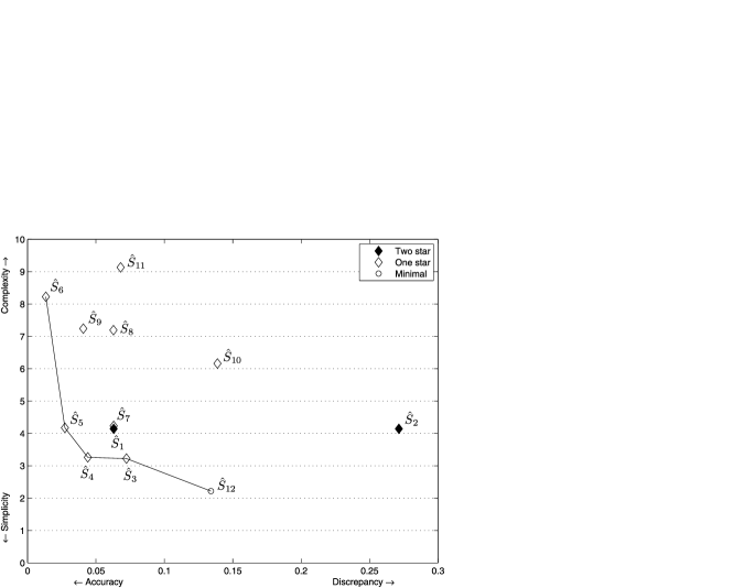
Figure 3: Solution set $\mathcal{S}$ for the exams data.

Figure 3 shows the corresponding scatterplot for the exams data where, overall, 12 different solutions were obtained. The numbering of the solutions reflects a particular principled order described below, together with the plot symbols used. In particular, the forwards solutions $\hat{S}(\theta^{[1]})$ and $\hat{S}(\theta^{[3]})$ discussed above appear here as $\hat{S}_{1}$ and $\hat{S}_{7}$, respectively.

2.4.2 Minimal and dominated solutions

Low values of both $\mathit{discr}(\hat{S})$ and $\mathit{compl}(\hat{S})$ are clearly desirable, but cannot usually be simultaneously achieved. For example, Figure 3 shows that there is a trade-off for the exams data, with no solution attaining the smallest value of both these coordinates. However, the five solutions joined by straight lines are visibly special, the rectangle formed by each of them with the origin containing no other solutions. For any set of solutions, we call these the minimal solutions—those for which no lower value of either coordinate can be found without increasing the other. Thus, here, among $\hat{S}_{3},\hat{S}_{4},\hat{S}_{5},\hat{S}_{6}$ and $\hat{S}_{12}$, the simpler solutions are less accurate, and the more accurate solutions are less simple.

There is always at least one minimal solution, usually more. Together, they form the lower-left boundary of the scatterplot whose shape reflects, in any particular case, the trade-off between simplicity and accuracy. All other solutions are dominated by a minimal solution. For example, here, $\hat{S}_{1}$ and $\hat{S}_{7}$ are dominated by $\hat{S}_{4}$, with $\hat{S}_{4}$ being simpler and more accurate than both.

2.4.3 Star quality solutions

In general, focusing only on solutions which lie in the minimal set does not necessarily capture all clearly interpretable solutions. Other, dominated, solutions may possess ‘star quality’ in the sense that there are striking overall patterns in the set of approximate axes found, deserving to be especially drawn to the user’s attention. For example, $\hat{S}_{1}$ (Table 4, repeated here as the left-hand part of Table 2.4.3) has a very clear and interpretable structure and so deserves to be brought early to the user’s attention, even though it does not lie in the minimal set. For many users this increased interpretability is likely to be worth the cost in terms of discrepancy and overall complexity.

We recognize that interpretability is a subjective concept. Rather than attempting a quantification, we use a star rating system to indicate the degree to which a solution conforms with one of a predefined set of clear structures: ‘two star’ solutions conform to the clearest structures and ‘one star’ to the next clearest, while ‘unstarred’ solutions do not conform to any of the predefined structures.

Here, we use six predefined structures, these being one and two star versions of three mutually exclusive types, denoted A, B and C, described next. There are clear points of contact with the work of Rousson and Gasser, summarized in the following Section 2.4.4.

=330pt $\bolds{\hat{\bolds{S}}_{1}}$ $\bolds{\hat{\bolds{S}}_{2}}$ Variable $\bolds{\hat{\mathbf{z}}_{1}}$, $\bolds{\hat{\mathbf{z}}_{2}}$0 $\bolds{\hat{\mathbf{z}}_{3}}$0 $\bolds{\hat{\mathbf{z}}_{4}}$0 $\bolds{\hat{\mathbf{z}}_{5}}$ $\bolds{\hat{\mathbf{z}}_{1}}$ $\bolds{\hat{\mathbf{z}}_{2}}$0 $\bolds{\hat{\mathbf{z}}_{3}}$0 $\bolds{\hat{\mathbf{z}}_{4}}$0 $\bolds{\hat{\mathbf{z}}_{5}}$0 Mechanics $1$ $1$ $1$ $0$ $1$ $1$ $1$ $1$ $1$ $0$ Vectors $1$ $1$ $-1$ $0$ $1$ $1$ $1$ $-1$ $1$ $0$ Algebra $1$ $0$ $0$ $0$ $-4$ $1$ $-1$ $0$ $1$ $1$ Analysis $1$ $-1$ $0$ $1$ $1$ $1$ $-1$ $0$ $1$ $-1$ Statistics $1$ $-1$ $0$ $-1$ $1$ $1$ $0$ $0$ $-4$ $0$ Accuracy $0.997$ $0.973$ $0.9375$ $0.937$ $0.974$ $0.997$ $0.802$ $0.9375$ $0.729$ $0.897$ Variance (%) $63.3$ $14.4$ $8.9$ $7.9$ $5.5$ $63.3$ $12.1$ $8.9$ $9.9$ $5.8$

Table 6: Integer representations of the two star solutions for the exams data

Let $\widehat{\mathbf{Z}}=(\hat{\mathbf{z}}_{1}|\cdots|\hat{\mathbf{z}}_{k})$ be a matrix of integer representations of $\hat{S}$. Each structure used requires that the $p$ variables can be partitioned into $b\geq 1$ blocks, where each block labels the set of nonzero (by convention, positive) elements of a single-signed column $\hat{\mathbf{z}}_{r}$. If $b<k$, orthogonality entails that the remaining $(k-b)$ columns of $\widehat{\mathbf{Z}}$ are contrasts—that is, have elements of both signs. The within-block condition W-B [condition 3 in Rousson and Gasser (2004)] holds if the nonzero elements of each contrast occur within a single block.

In this terminology, the three mutually exclusive types of predefined structure are as follows:

A:

$b=1$—that is, an overall (possibly, weighted) mean, plus orthogonal contrasts.

B:

$b>1$ and W-B holds, so that each block has type A structure.

C:

$b>1$ and W-B does not hold.

The type of each starred solution is noted in its table of information but, for visual clarity, not in the accuracy–simplicity scatterplot.

We call $\hat{\mathbf{z}}_{r}$ parsimonious if $N_{r}^{\sharp}$, the number of distinct nonzero elements it contains, is small. The more parsimonious a starred solution, the clearer its structure. Accordingly, we award two stars when it is as parsimonious as possible of its type, and one star otherwise. Orthogonality entails that, for each type, two star solutions are precisely those which obey the following two conditions:

$$\max\{N_{r}^{\sharp}\dvtx\hat{\mathbf{z}}_{r}\mbox{ defines a block}\} = 1\quad\mbox{and}$$

$$\max\{N_{r}^{\sharp}\dvtx\hat{\mathbf{z}}_{r}\mbox{ defines a contrast}\} = 2.$$

For example, adopting an obvious notation, an A^∗∗ solution has a simple arithmetic mean, plus a set of orthogonal contrasts in each of which the nonzero elements comprise $m$ times a value $n$, and $n$ times a value $-m$, whereas an A^∗ solution has either an unequally weighted mean, or a contrast not of this form.

Examples of the six possible starred structures are given below, the A^∗ example being $\hat{S}_{3}$ in Figure 3 and detailed in the left-hand part of Table 2.4.4.

	Structure type
	A	B	C
Two star	${{\left(\matrix{1&\phantom{-}1&\phantom{-}1&\phantom{-}0&\phantom{-}1\cr 1&\phantom{-}1&-1&\phantom{-}0&\phantom{-}1\cr 1&\phantom{-}0&\phantom{-}0&\phantom{-}0&-4\cr 1&-1&\phantom{-}0&\phantom{-}1&\phantom{-}1\cr 1&-1&\phantom{-}0&-1&\phantom{-}1}\right)}}$	${{\left(\matrix{1&0&\phantom{-}1&\phantom{-}0\cr 1&0&-1&\phantom{-}0\cr 0&1&\phantom{-}0&\phantom{-}1\cr 0&1&\phantom{-}0&-1}\right)}}$	${{\left(\matrix{1&0&\phantom{-}1&\phantom{-}1\cr 1&0&-1&-1\cr 0&1&\phantom{-}1&-1\cr 0&1&-1&\phantom{-}1}\right)}}$
One star	${{\left(\matrix{3&-1&\phantom{-}1&\phantom{-}0&\phantom{-}0\cr 3&-1&-1&\phantom{-}0&\phantom{-}0\cr 2&\phantom{-}1&\phantom{-}0&\phantom{-}0&-2\cr 2&\phantom{-}1&\phantom{-}0&\phantom{-}1&\phantom{-}1\cr 2&\phantom{-}1&\phantom{-}0&-1&\phantom{-}1}\right)}}$	${{\left(\matrix{1&0&\phantom{-}2&\phantom{-}0\cr 2&0&-1&\phantom{-}0\cr 0&1&\phantom{-}0&\phantom{-}2\cr 0&2&\phantom{-}0&-1}\right)}}$	${{\left(\matrix{1&0&\phantom{-}2&\phantom{-}2\cr 2&0&-1&-1\cr 0&1&\phantom{-}2&-2\cr 0&2&-1&\phantom{-}1}\right)}}$

2.4.4 Empirical support for assumed models: Points of contact with Rousson and Gasser

Our approach seeks solutions supported by the data in the sense that no modeling assumptions are imposed, apart from our axes being orthogonal and containing vectors of integers. Therefore, if an optimal solution under some modeling assumptions is produced by our analysis, this provides empirical evidence in favor of such a model.

We develop this general point here with respect to the Rousson and Gasser method, as reported in Rousson and Gasser (2004), with which there are clear points of contact, recalling that it applies to correlation matrices only.

=330pt $\bolds{\hat{S}_{1}}$ $\bolds{\hat{S}_{2}}$ Variable $\bolds{\hat{\mathbf{z}}_{1}}$, $\bolds{\hat{\mathbf{z}}_{2}}$0 $\bolds{\hat{\mathbf{z}}_{3}}$ $\bolds{\hat{\mathbf{z}}_{4}}$ $\bolds{\hat{\mathbf{z}}_{5}}$ $\bolds{\hat{\mathbf{z}}_{1}}$ $\bolds{\hat{\mathbf{z}}_{2}}$0 $\bolds{\hat{\mathbf{z}}_{3}}$0 $\bolds{\hat{\mathbf{z}}_{4}}$0 $\bolds{\hat{\mathbf{z}}_{5}}$0 Mechanics $3$ $-1$ $1$ $0$ $0$ $1$ $3$ $2$ $1$ $0$ Vectors $3$ $-1$ $-1$ $0$ $0$ $1$ $3$ $-2$ $-1$ $0$ Algebra $2$ $1$ $0$ $0$ $-2$ $1$ $-2$ $0$ $0$ $-2$ Analysis $2$ $1$ $0$ $1$ $1$ $1$ $-2$ $-1$ $2$ $1$ Statistics $2$ $1$ $0$ $-1$ $1$ $1$ $-2$ $1$ $-2$ $1$ Accuracy $0.996$ $0.928$ $0.937$ $0.937$ $0.959$ $0.997$ $0.956$ $0.98$ $0.978$ $0.959$ Variance (%) $60.2$ $17.3$ $8.9$ $7.9$ $5.7$ $63.3$ $14.2$ $8.9$ $7.8$ $5.7$

Table 7: Integer representations of the two best one star approximations for exams data

A key point is that two star structures emerging from our essentially exploratory analysis of the data correspond to assumed structures optimally fitted to it in Rousson and Gasser (2004), with the added condition of orthogonality between all pairs of approximate axes. Accordingly, solutions generated by Rousson and Gasser (2004) can only coincide with ours when they are orthogonal, in which case they are two star solutions. In particular, one star solutions—involving weighted means and/or contrasts not of the A^∗∗ form noted above—cannot arise in such an analysis.

For any given number of blocks $b$, the scalar target function optimized in Rousson and Gasser (2004)—the ‘corrected sum of variances’ [see the paper by Gervini and Rousson (2004)], denoted here by $\mathit{optim}(\hat{S})$—can be used whether components are orthogonal or not. Although not optimized for in our approach, its value can be calculated for each of our solutions and compared to the best value found in Rousson and Gasser (2004). However, its maximization reflects an exclusive interest in explaining variability, whereas, being as interested in exploring potential scientific laws, our approach treats all eigenvectors of interest equally.

Overall, the two methods will give complementary results, agreement only being expected when there is strong empirical evidence of an orthogonal two star structure underpinning the variability in the data.

2.4.5 A total order of solutions

A principled total order of the full set of solutions $\mathcal{S}$ is now obtained, in two stages.

First, we place each solution into one of four classes, ordered by interpretability: two star solutions, one star solutions, unstarred solutions lying in the minimal set for $\mathcal{S}$, and the rest. All solutions in a higher class are ranked ahead of all those in a lower class.

Then, we order the solutions within each class by simplicity and accuracy, with our usual bias toward the former, as follows. Having found the minimal set for a given class, we give its solutions the highest available rankings, ordering them by $\mathit{compl}(\hat{S})$ [any ties being broken by $\mathit{discr}(\hat{S})$]—in other words, working from right to left in the accuracy–simplicity scatterplot. We now remove this minimal set from the class and repeat the ranking procedure on the remainder until all solutions in the class have been ranked.

Tabular information for each solution is presented to the user in the resulting total order. For visual clarity, solutions in the lowest class—those neither starred, nor minimal for $\mathcal{S}$—are not numbered in the scatterplot.

For example, for the exams data, the two star class comprises $\hat{S}_{1}$ and $\hat{S}_{2}$ (shown in Table 2.4.3), reflecting the fact that they are considered top in terms of interpretability. Both are of type A. Between them, $\hat{S}_{1}$ is ranked higher as it dominates $\hat{S}_{2}$, having the same overall complexity but a much better minimum accuracy attained: $0.937$ compared to $0.729$ (for the fourth axis in both cases). Indeed, the corresponding angle for this axis being some $43^{\circ}$, it seems likely that many users will rule out $\hat{S}_{2}$ as being insufficiently accurate.

The one star class comprises solutions $\hat{S}_{3}$ to $\hat{S}_{11}$. Among them, solutions $\hat{S}_{3}$–$\hat{S}_{6}$ have the highest rankings since they form the corresponding minimal set—that is, within this class, it is not possible to improve on either overall simplicity or accuracy without doing worse on the other criterion. They are ranked by overall simplicity [small values of $\mathit{compl}(\hat{S})$]. Removing them from the class and continuing, the new (ordered) minimal classes are $\hat{S}_{7}$ to $\hat{S}_{9}$ and, finally, $\hat{S}_{10}$ and $\hat{S}_{11}$. For the exams data, $\hat{S}_{12}$ is the only unstarred solution in the minimal set for $\mathcal{S}$, while there are no solutions in the lowest class.

2.5 Running example: Summary comparison of results

We summarize here our results for the exam data running example (Section 1.4) displayed in Figure 3, whose terminology is explained above, comparing them with those of Rousson and Gasser (2004) and Vines (2000).

Overall, the user is referred first to $\hat{S}_{1}$, shown in the left part of Table 2.4.3. This effectively combines simplicity, accuracy and subject matter interpretability, this latter being particularly straightforward:

Represents overall mathematical ability.

Contrasts closed- and open-book exam performance, omitting Algebra.

Contrasts performance in the two closed-book exams, Mechanics and Vectors.

Contrasts performance in the two open-book exams, Analysis and Statistics, included in $\hat{\alpha}_{2}$.

Contrasts Algebra with all other subjects.

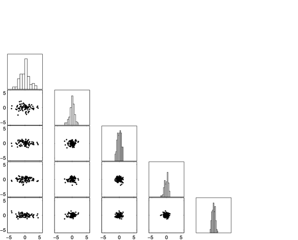
Figure 4: Scatterplot matrix of the simplified principal components for the exams data.

Figure 4 shows the scatterplot matrix for $\hat{S}_{1}$, the visualization and dimension reduction features offered by such orthogonal-axis plots only being guaranteed with rotation approaches such as ours. The performance of each student on each of these five readily interpreted axes is visible. In particular, two or three students stand out at either extreme of overall mathematical ability, these students having very similar open- and closed-book performances as measured by $\hat{\alpha}_{2}$. Again, we can see at once that there are no great correlations induced by this simplification—in fact, the two largest absolute correlations between the simple components are about $0.2$, for $(\hat{\alpha}_{1},\hat{\alpha}_{5})$ and $(\hat{\alpha}_{1},\hat{\alpha}_{4})$, respectively. Overall, the scatterplot matrix is visually close to the one given by an exact principal component analysis, but much more interpretable.

Skipping $\hat{S}_{2}$, the two best one star solutions, $\hat{S}_{3}$ and $\hat{S}_{4}$, again both of type A, are shown in Table 2.4.4. They remain clearly interpretable, having greater overall simplicity than $\hat{S}_{1}$ and comparable accuracies to it (indeed, $\hat{S}_{4}$ dominates $\hat{S}_{1}$). In particular, the first two simple components comprise an overall mean and an open-closed book contrast, $\hat{S}_{3}$ using a weighted mean and $\hat{S}_{4}$ a weighted contrast. Between them, our automated bias toward simplicity puts $\hat{S}_{3}$ first. In it, all other contrasts are either within closed-book exams ($\hat{\mathbf{z}}_{3}$) or within open-book exams ($\hat{\mathbf{z}}_{4}$ and $\hat{\mathbf{z}}_{5}$). Overall, $\hat{S}_{3}$ and $\hat{S}_{4}$ provide helpful, alternative views of the same data. As noted above (Section 2.4.4), Rousson and Gasser (2004) will not report such one star solutions.

The default version of Rousson and Gasser (2004) estimates one block to be appropriate for this data set. Our $\hat{S}_{1}$ solution coincides with their corresponding optimal $b=1$ fit, providing empirical support for its implicit model (see Section 2.4.4). Although orthogonal, their optimal $b=2$ fit does not appear among our solutions, adding further empirical evidence that a two block model is not appropriate for these data.

The method of Vines (2000) with associated parameter $c=0$ produces the same first and third components as our $\hat{S}_{1}$. Its other components differ and are somewhat harder to interpret, the highest complexity (11 for component 4) exceeding $N^{\ast}=9$.

3 Further examples

3.1 Reflexes data

The reflexes data, taken from Section 3.8.1 of Jolliffe (2002), comprise measurements on 143 individuals of left and right reflexes for five parts of the body, three in the upper limb and two in the lower.

Table 8: Exact PCA loadings (rounded to 2 decimal places) for the reflexes data

Variable	$\mathbf{q_{1}}$	$\mathbf{q_{2}}$	$\mathbf{q_{3}}$	$\mathbf{q_{4}}$	$\mathbf{q_{5}}$	$\mathbf{q_{6}}$	$\mathbf{q_{7}}$	$\mathbf{q_{8}}$	$\mathbf{q_{9}}$	$\mathbf{q_{10}}$
triceps.R	$0.35$	$-0.18$	$0.18$	$0.49$	$-0.27$	$-0.06$	$-0.05$	$0.00$	$0.10$	$0.69$
triceps.L	$0.36$	$-0.19$	$0.15$	$0.47$	$-0.27$	$-0.02$	$-0.13$	$0.01$	$-0.13$	$-0.70$
biceps.R	$0.36$	$-0.13$	$-0.14$	$0.04$	$0.71$	$-0.50$	$-0.22$	$-0.03$	$-0.19$	$0.04$
biceps.L	$0.39$	$-0.14$	$-0.09$	$0.05$	$0.41$	$0.70$	$0.35$	$0.02$	$0.19$	$-0.03$
wrist.R	$0.34$	$-0.24$	$0.14$	$-0.51$	$-0.16$	$-0.21$	$-0.13$	$-0.01$	$0.67$	$-0.10$
wrist.L	$0.34$	$-0.22$	$0.17$	$-0.52$	$-0.23$	$0.11$	$0.08$	$0.03$	$-0.67$	$0.12$
knee.R	$0.30$	$0.29$	$-0.50$	$0.02$	$-0.24$	$-0.35$	$0.62$	$-0.02$	$0.01$	$-0.04$
knee.L	$0.27$	$0.35$	$-0.54$	$-0.07$	$-0.18$	$0.28$	$-0.63$	$0.02$	$-0.02$	$0.06$
ankle.R	$0.20$	$0.53$	$0.41$	$-0.03$	$0.07$	$0.03$	$0.00$	$-0.71$	$-0.01$	$-0.02$
ankle.L	$0.19$	$0.54$	$0.40$	$-0.02$	$0.10$	$-0.04$	$0.01$	$0.70$	$0.03$	$-0.01$
Variance (%)	$52.23$	$20.36$	$10.94$	$8.57$	$4.96$	$1.08$	$0.86$	$0.59$	$0.23$	$0.19$

A principal component analysis of the correlation matrix is reported in Table 8. This brings out some of the structure in the data. It also provides a further example of the appropriateness of taking equal scientific interest in all the components.

The dominant component is an overall mean, while components 2–5 contrast reflexes in different parts of the body. Smaller components mainly contrast reflexes on the left and right sides of the body, the substantially smaller variances associated with them suggesting near constant linear relationships. However, more detailed interpretation of the principal components is not immediate. For example, interpretation of the first principal component is impaired by variability in the loadings, notably the relatively small ones allocated to the two ankle measurements.

3.1.1 Results of our approach

Our approach provides six different solutions for these data. The corresponding accuracy–simplicity plot (Figure 5) shows $\hat{S}_{1}$ and $\hat{S}_{2}$ with two stars, $\hat{S}_{3}$ and $\hat{S}_{4}$ with one star, $\hat{S}_{5}$ as an unstarred minimal solution, and one unlabeled ‘other’ solution $\hat{S}_{6}$.

Figure 5: Solution set $\mathcal{S}$ for the reflexes data.

The user is referred first to solution $\hat{S}_{1}$, shown in Table 3.1.1, which has the following clear interpretation. The dominant simple component $\hat{\alpha}_{1}$ is just the simple average of all the reflexes, while $\hat{\alpha}_{2}$ contrasts those in upper and lower limbs. Again, $\hat{\alpha}_{3}$ contrasts the two lower limb parts, while $\hat{\alpha}_{4}$ and $\hat{\alpha}_{5}$ contrast the three upper limb parts: first, triceps with wrist; then, biceps with these two. Taking the near constant simple components in reverse order, $\hat{\alpha}_{10}$ to $\hat{\alpha}_{8}$ suggest left–right symmetry in triceps, wrist and ankle respectively. Finally, taking $\hat{\alpha}_{7}$ and $\hat{\alpha}_{6}$ together as we may (they have essentially the same variance), the two-dimensional subspace which they span suggests left–right symmetry in knees and biceps. This follows at once from considering their sum and difference, corresponding to a $45^{\circ}$ rotation of axes within this subspace.

The variance explained by the first five simple components here is $96.7\%$ compared to $97.1\%$ for the exact principal components, each being close to that of its optimal counterpart. There are three absolute correlations of about $0.3$ [for $(\hat{\alpha}_{5},\hat{\alpha}_{7})$, $(\hat{\alpha}_{6},\hat{\alpha}_{9})$ and $(\hat{\alpha}_{7},\hat{\alpha}_{9})$], all others being appreciably smaller.

=330pt Variable $\bolds{\hat{\mathbf{z}}_{1}}$ $\bolds{\hat{\mathbf{z}}_{2}}$ $\bolds{\hat{\mathbf{z}}_{3}}$ $\bolds{\hat{\mathbf{z}}_{4}}$ $\bolds{\hat{\mathbf{z}}_{5}}$ $\bolds{\hat{\mathbf{z}}_{6}}$ $\bolds{\hat{\mathbf{z}}_{7}}$ $\bolds{\hat{\mathbf{z}}_{8}}$ $\bolds{\hat{\mathbf{z}}_{9}}$ $\bolds{\hat{\mathbf{z}}_{10}}$ triceps.R $1$ $2$ $1$ $1$ $-1$ triceps.L $1$ $2$ $1$ $1$ $1$ biceps.R $1$ $2$ $-2$ $-1$ $1$ biceps.L $1$ $2$ $-2$ $1$ $-1$ wrist.R $1$ $2$ $-1$ $1$ $-1$ wrist.L $1$ $2$ $-1$ $1$ $1$ knee.R $1$ $-3$ $-1$ $-1$ $-1$ knee.L $1$ $-3$ $-1$ $1$ $1$ ankle.R $1$ $-3$ $1$ $-1$ ankle.L $1$ $-3$ $1$ $1$ Accuracy $0.98$ $0.95$ $0.92$ $0.99$ $0.91$ $0.91$ $0.91$ $0.998$ $0.95$ $0.98$ Variance (%) $50.8$ $20.6$ $11.2$ $8.6$ $5.6$ $1.1$ $1.1$ $0.6$ $0.3$ $0.2$ []Notes:Reflexesdata.Emptyentriesmeanzeroes.

Table 9: Integer representations for $\hat{S}_{1}$

The one star solution $\hat{S}_{3}$ is very close to $\hat{S}_{1}$ in Figure 5. Indeed, it differs from it only in $\hat{\alpha}_{6}$ and $\hat{\alpha}_{7}$ representing another rotation within their span, already interpreted above as suggesting left–right symmetry in knees and biceps. This time, at the cost of increasing the complexity of both $\hat{\alpha}_{6}$ and $\hat{\alpha}_{7}$ by one, their accuracies improve to $0.95$ and $0.97$, respectively. This illustrates that subspace rotation can increase accuracy without changing overall interpretation.

Although dominated by $\hat{S}_{1}$, the other two star solution $\hat{S}_{2}$ provides an interesting alternative view. It differs only on two components, both having very clear interpretations:

Contrasts upper and lower limbs, omitting biceps, using only $\pm 1$ loadings.

Contrasts biceps with everything else, using only 1 and $-4$ loadings.

The other, unstarred, minimal solution $\hat{S}_{5}$ (details not shown) is simple and accurate, but somewhat less clearly structured. Its $\hat{\alpha}_{4}$ and $\hat{\alpha}_{8}$ to $\hat{\alpha}_{10}$ agree exactly with $\hat{S}_{1}$, the sign pattern of $\hat{\alpha}_{6}$ and $\hat{\alpha}_{7}$ also agreeing (each now has loadings of $\pm 2$). $\hat{\alpha}_{1}$ is a weighted mean, omitting ankle. $\hat{\alpha}_{5}$ also omits ankle, contrasting biceps with the other three body parts. $\hat{\alpha}_{2}$ contrasts upper and lower limbs, omitting biceps. Finally, $\hat{\alpha}_{3}$ also omit biceps, contrasting knee with the other three body parts.

The other two solutions, $\hat{S}_{4}$ and $\hat{S}_{6}$, are markedly less simple and accurate.

3.1.2 Comparison with other approaches

We briefly compare our results here with those of other methods.

The comparison with Rousson and Gasser’s approach for these data is, essentially, the same as it was for the running exams data (see the end of Section 2.5). The default version of Rousson and Gasser (2004) again estimates $b=1$, our $\hat{S}_{1}$ solution coinciding with their corresponding optimal fit, providing empirical support for its implicit model. Although orthogonal, their optimal $b=2$ fit does not appear among our solutions, adding further empirical evidence that a two block model is not appropriate for these data.

Table 10: Integer representations for the reflexes data using Vines’ method with $c=0$

Variable	$\bolds{\hat{\mathbf{z}}_{1}}$	$\bolds{\hat{\mathbf{z}}_{2}}$	$\bolds{\hat{\mathbf{z}}_{3}}$	$\bolds{\hat{\mathbf{z}}_{4}}$	$\bolds{\hat{\mathbf{z}}_{5}}$	$\bolds{\hat{\mathbf{z}}_{6}}$	$\bolds{\hat{\mathbf{z}}_{7}}$	$\bolds{\hat{\mathbf{z}}_{8}}$	$\bolds{\hat{\mathbf{z}}_{9}}$	$\bolds{\hat{\mathbf{z}}_{10}}$
triceps.R	$1$	$1$	$2$	$1$	$19$	$-19$	$19$	$19$	$-19$	$-1$
triceps.L	$1$	$1$	$2$	$1$	$19$	$-19$	$19$	$19$	$-19$	$1$
biceps.R	$1$	$1$	$-1$		$-42$	$-2479$	$-42$	$-42$	$42$
biceps.L	$1$	$1$	$-1$		$-40$	$2561$	$-40$	$-40$	$40$
wrist.R	$1$	$1$	$2$	$-1$	$18$	$-19$	$19$	$18$	$-2541$
wrist.L	$1$	$1$	$2$	$-1$	$20$	$-19$	$19$	$20$	$2503$
knee.R	$1$	$-1$	$-9$		$10$	$-9$	$-2512$	$10$	$-10$
knee.L	$1$	$-1$	$-9$		$8$	$-9$	$2530$	$8$	$-8$
ankle.R	$1$	$-2$	$6$		$-5$	$6$	$-6$	$-2529$	$6$
ankle.L	$1$	$-2$	$6$		$-7$	$6$	$-6$	$2517$	$6$
Accuracy	$0.98$	$0.97$	$0.99$	$0.99$	$0.97$	$0.85$	$0.89$	$1.00$	$0.95$	$0.98$
Variance (%)	$50.8$	$21.5$	$11$	$8.6$	$5$	$1.2$	$0.99$	$0.60$	$0.30$	$0.20$

[]Note: Empty entries mean zeroes.

Table 3.1.2 shows the components obtained using the method of Vines (2000) with associated parameter $c=0$. Compared to the original principal component analysis (Table 8), this gives a substantially simpler, more interpretable solution. It differs from $\hat{S}_{1}$, especially for middle components, but interestingly picks up the same simplified components $\hat{\alpha}_{1}$, $\hat{\alpha}_{4}$ and $\hat{\alpha}_{10}$, interpreted above (this might, in part, be because Vines’ method is able to seek simplifications of components in a nonsequential fashion). Axes $\hat{\alpha}_{8}$ and $\widehat{\alpha}_{9}$ here have virtually the same accuracy as in $\hat{S}_{1}$ but are much more complex, illustrating that our bias toward simplicity does not necessarily sacrifice accuracy. Indeed, having a dominant pair of elements of nearly equal size and opposite sign, $\hat{\alpha}_{8}$ and $\hat{\alpha}_{9}$ are both angle-close to the corresponding axes in $\hat{S}_{1}$, interpreted above as suggestive of left–right symmetry in the corresponding part of the body. By the same token, $\hat{\alpha}_{6}$ and $\hat{\alpha}_{7}$ are also angle-close to suggesting corresponding left–right symmetries. The remaining axes, $\hat{\alpha}_{2}$, $\hat{\alpha}_{3}$ and $\hat{\alpha}_{5}$, are more accurate, but less directly interpretable, than those in $\hat{S}_{1}$.

=280pt Variable $\mathbf{q_{1}}$ $\mathbf{q_{2}}$ $\mathbf{q_{3}}$ $\mathbf{q_{4}}$ Length $0.25$ $0.03$ $0.02$ $0.07$ Width $0.26$ $0.07$ $0.01$ $0.10$ Forwing $0.26$ $0.03$ $-0.05$ $0.07$ Hinwing $0.26$ $0.09$ $0.03$ $0.00$ Antseg 1 $0.24$ $-0.18$ $0.04$ $-0.01$ Antseg 2 $0.25$ $-0.16$ $0.00$ $0.02$ Antseg 3 $0.23$ $0.24$ $0.05$ $0.11$ Antseg 4 $0.24$ $0.04$ $0.16$ $0.01$ Antseg 5 $0.25$ $-0.03$ $0.10$ $-0.02$ Tarsus 3 $0.26$ $0.01$ $0.03$ $0.18$ Tibia 3 $0.26$ $0.03$ $0.08$ $0.20$ Femur 3 $0.26$ $0.07$ $0.12$ $0.19$ Rostrum $0.25$ $-0.01$ $0.07$ $0.04$ Ovipositor $0.20$ $-0.40$ $-0.02$ $0.06$ Spiracles $0.16$ $-0.41$ $-0.19$ $-0.62$ Ov-spines $0.11$ $-0.55$ $-0.15$ $0.04$ Anal fold $-0.19$ $-0.35$ $0.04$ $0.49$ Ant-spines $-0.13$ $-0.20$ $0.93$ $-0.17$ Hooks $0.20$ $0.28$ $0.05$ $-0.45$ Variance (%) $73.0$ $12.5$ $3.9$ $2.6$

Table 11: Exact principal component analysis loadings (rounded to 2 decimal places) for the alate adelges data

3.2 Alate adelges data

These data consist of 19 anatomical measurements of 40 alate adelges (winged aphids), as reported in Jeffers (1967). The measurements taken on each aphid are its length and width, fore-wing and hind-wing lengths, 5 antennal segment lengths, 3 leg bone measurements, measurements of the rostrum and the ovipositor, anal fold, and counts of the number of spiracles, ovipositor spines, antennal spines and hind-wing hooks.

Jeffers (1967) focuses attention on the $k=4$ dominant eigenvectors of the correlation matrix shown in Table 11, these accounting for $92\%$ of the total variability in the data. He interprets $\alpha_{1}$ as a general index of size, and $\alpha_{2}$ to $\alpha_{4}$ as essentially measuring the number of ovipositor spines, of antennal spines and of spiracles, respectively.

These tidy interpretations are not without difficulty. For $\alpha_{1}$, some later variables have notably smaller loadings, of both signs. For each other $\alpha_{r}$, the interpretation offered amounts to ‘thresholding’ (setting all smaller loadings to zero) at the maximum absolute value of $q_{r}$. Whereas this looks quite reasonable for $\alpha_{3}$, it seems much less so for $\alpha_{2}$ and $\alpha_{4}$, these axes containing a range of substantial loadings, some of comparable magnitude to their maximum.

Inspection of the correlation matrix in Jeffers (1967) shows that, while positively correlated with each other, the two variables with negative loadings on $\alpha_{1}$ are, with one insignificant exception, negatively correlated with all the other variables. Indeed, a single negative (at $-0.026$, essentially zero) correlation remains when both their signs are reversed. Following Rousson and Gasser (2003), one strategy is to reverse these two signs, analyze the data in some way and then, to retain the interpretation of the original variables, switch them back again. We call this process ‘sign reversal.’

We compare here three solutions for these data, detailed in Table 3.2:

• $\hat{S}_{1}$, as defined above,

• $\widetilde{S}_{1}$, the result of an $\hat{S}_{1}$ analysis with sign reversal, and

• $\widetilde{S}_{\mathit{RG}}$, an optimal Rousson and Gasser (2004) fit with $b=1$ and, again, sign reversal.

Vines’ method is not capable to produce any answer here, mainly due to the complexity of some of the approximate loading vectors growing far too big.

Whereas none is ideal (in particular, there is substantial correlation in each, especially $\hat{S}_{1}$), these three solutions provide helpful, complementary views of these data. We discuss them in turn.

Table 12: Integer representations for the alate adelges data

	$\bolds{\hat{S}_{1}}$				$\bolds{\widetilde{S}_{1}}$				$\bolds{\widetilde{S}_{\mathit{RG}}}$
Variable	$\bolds{\hat{\mathbf{z}}_{1}}$	$\bolds{\hat{\mathbf{z}}_{2}}$	$\bolds{\hat{\mathbf{z}}_{3}}$	$\bolds{\hat{\mathbf{z}}_{4}}$	$\bolds{\hat{\mathbf{z}}_{1}}$	$\bolds{\hat{\mathbf{z}}_{2}}$	$\bolds{\hat{\mathbf{z}}_{3}}$	$\bolds{\hat{\mathbf{z}}_{4}}$	$\bolds{\hat{\mathbf{z}}_{1}}$	$\bolds{\hat{\mathbf{z}}_{2}}$	$\bolds{\hat{\mathbf{z}}_{3}}$	$\bolds{\hat{\mathbf{z}}_{4}}$
Length	$1$				$2$				$1$		$3$
Width	$1$				$2$				$1$		$3$	$1$
Forwing	$1$				$2$				$1$			$1$
Hinwing	$1$				$2$				$1$		$3$
Antseg 1	$1$				$2$	$1$			$1$
Antseg 2	$1$				$2$	$1$			$1$
Antseg 3	$1$	$-1$			$2$	$-1$			$1$	$3$	$3$	$1$
Antseg 4	$1$				$2$				$1$		$3$
Antseg 5	$1$				$2$				$1$		$3$
Tarsus 3	$1$				$2$	$-1$		$1$	$1$		$3$	$1$
Tibia 3	$1$				$2$			$1$	$1$		$3$	$1$
Femur 3	$1$				$2$			$1$	$1$		$3$	$1$
Rostrum	$1$				$2$				$1$		$3$
Ovipositor	$1$	$1$			$1$	$2$			$1$	$-4$		$1$
Spiracles		$1$		$1$		$2$	$1$	$-2$	$1$	$-4$	$-11$	$-3$
Ov-spines		$1$			$1$	$2$			$1$	$-4$	$-11$	$1$
Anal fold		$1$		$-1$	$-1$	$2$		$2$	$-1$	$-3$		$3$
Ant-spines			$1$			$1$	$-2$	$-1$	$-1$	$-3$	$11$	$-1$
Hooks				$1$	$2$	$-1$		$-2$	$1$	$3$	$3$	$-3$
Accuracy	$0.93$	$0.87$	$0.93$	$0.90$	$0.97$	$0.95$	$0.92$	$0.96$	$0.98$	$0.94$	$0.75$	$0.96$
Variance (%)	$63.5$	$9.7$	$5.3$	$9.8$	$69$	$11.6$	$6$	$2.7$	$70.2$	$11.3$	$7.8$	$3$
Optimality (%)	$86.9$				$94.1$				$94.5$
Max correl	$0.83$				$0.63$				$0.63$

[]

Note:Emptyentriesmeanzeroes.

As expected, given that $\alpha_{1}$ is not single-signed, $\hat{S}_{1}$ is unstarred. Nevertheless, it is perhaps the most easily interpreted solution. It is the simplest and sparsest, all loadings being 0, 1 or $-1$. Its dominant component is the simple average of all the variables, excluding the four count variables and anal fold. Its third component is the number of antennal spines. The other two components are simple contrasts, whose pattern of zeroes is consistent with thresholding at lower levels with only two exceptions (the last two loadings in $\hat{\alpha}_{2}$), these zeroes ensuring orthogonality. However, $\hat{\alpha}_{2}$ is not very accurate and, indeed, explains less variance than $\hat{\alpha}_{4}$.

$\widetilde{S}_{1}$ is the most accurate solution, the minimum accuracy being 0.92. Although also unstarred, it is perhaps the next most easily interpreted. It is nearly as simple and as sparse as $\hat{S}_{1}$. It has a comparable corrected sum of variances to the optimized $\widetilde{S}_{\mathit{RG}}$ fit (94.1% compared to 94.5%), achieved despite having lower variances associated with the last two components, consistent with their suggestion of underlying regularities. Compared to $\hat{S}_{1}$, its dominant component gains accuracy and variance explained, but is less easily interpreted. Finally, the pattern of zeroes in its other components is consistent with thresholding at yet lower levels with only one exception (for Tarsus 3 on $\hat{\alpha}_{2}$), this nonzero loading ensuring orthogonality.

A $b=1$ solution such as $\widetilde{S}_{\mathit{RG}}$ comes from fitting the following assumed form of two star solution to the (sign reversed) data: a simple arithmetic mean, plus a set of contrasts in each of which the nonzero elements comprise $m$ times a value $n$, and $n$ times a value $-m$. As happens here, these contrasts need not be orthogonal, so that $\widetilde{S}_{\mathit{RG}}$ cannot appear among our solutions. Its dominant component fits well, having the highest accuracy and variance explained, while the zeroes in its second component are, without exception, consistent with the same lower thresholding as in $\hat{S}_{1}$. However, the other fits seem poor, $\hat{\alpha}_{3}$ having a particularly low accuracy, while $\hat{\alpha}_{4}$ is considerably less sparse than in $\widetilde{S}_{1}$ but without improving accuracy. Overall, despite dropping the orthogonality constraint, $\widetilde{S}_{\mathit{RG}}$ comes third in terms of simplicity, accuracy and sparseness. A likely reason for this is that its assumed model seems, at most, appropriate to the first two components.

3.3 Larger data sets

In this section we use simulated examples to give an idea of how our method behaves when the number of variables $p$ grows. These examples also illustrate the secondary, initially surprising, fact that certain simple structures in the population principal components can be recovered using only information from the sample. Such behavior has been observed, for small dimensions, in one other simplification method: see Sun (2006).

For $p=$ 8, 16, 32, 64, 128 and 256, we simulated 100 data sets of size $n$ from a $p$-variate, zero mean, normal distribution with covariance matrix of the following form. Its matrix $\mathbf{Q}_{\mathrm{pop}}$ of population eigenvectors is the particular integer matrix with orthogonal columns $\mathbf{Z}_{\mathrm{pop}}$ detailed below, normalized to unit column length. Its spectrum has four reasonably well-separated dominant eigenvalues $(16,8,4,2)$, the rest being equal with sum $1$. Thus, for each $p$, the first four population components explain $30/31\sim 97\%$ of total variability, the corresponding four sample components being used as input data here in each case. Sampling variability was kept constant across different values of $p$ in the sense that the ratio of the number of degrees of freedom in the centered data to that in $\mathbf{Q}_{\mathrm{pop}}$ was kept fixed at $8$, giving $n=4p-3$.

We use the following two star structure for the population eigenaxes generated by $\mathbf{Z}_{\mathrm{pop}}$. A so-called Hadamard matrix of order $p=2^{m}$ can be obtained inductively using

$$\mathbf{Z}_{\mathrm{pop}}(2)=\pmatrix{1&1\cr 1&-1}$$

and

$$\mbox{for }m>1\qquad\mathbf{Z}_{\mathrm{pop}}(2^{m})=\pmatrix{\mathbf{Z}_{\mathrm{pop}}(2^{m-1})&\mathbf{Z}_{\mathrm{pop}}(2^{m-1})\cr\mathbf{Z}_{\mathrm{pop}}(2^{m-1})&-\mathbf{Z}_{\mathrm{pop}}(2^{m-1})}.$$

For example, this gives

$$\mathbf{Z}_{\mathrm{pop}}(4)=\pmatrix{1&1&1&1\cr 1&-1&1&-1\cr 1&1&-1&-1\cr 1&-1&-1&1}$$

(axis-equivalent to that found in the blood flow data of Section 1.3.2). This structure is the opposite of sparse, having no zeroes. Instead, it has what Chipman and Gu (2005) call ‘homogeneity.’ At the same time, it is extremely simple. For any $m$, the $\lambda$ part of our overall complexity measure (Section 2.4.1) takes its maximum value $1/2$, so that $\mathit{compl}(S_{\mathrm{pop}})=1.5$ if and only if $\mathbf{Z}_{\mathrm{pop}}$ has this Hadamard form.

Figure 6 shows that the computation time required grows roughly linearly in $p$, which gives a good indication that the method is relatively quick when $p\leq 256$ and there is a simple structure in the sample eigenvectors.

Figure 7 is an accuracy–simplicity scatterplot for the $100$ simulated values of $\hat{S}_{1}$ obtained with $p=32$. The percentage of simulations with $\mathit{compl}(\hat{S}_{1})=1.5$, corresponding to $\hat{S}_{1}$ having a Hadamard structure, is substantial. Overall, this percentage was found to increase with $p$, as was the minimum accuracy attained.

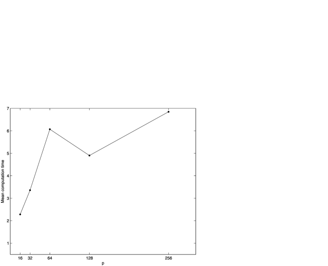
Figure 6: Mean computation times relative to the time for $p=8$.

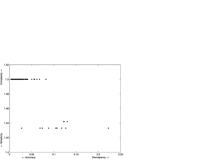
Figure 7: Accuracy and complexity for solution to simulated data when $p=32$.

4 Discussion

Combining principles with pragmatism, a new approach and accompanying algorithm to interpret (a subset of) principal components have been presented and shown to work well on a range of examples. The key idea is to approximate each eigenvector involved by an integer vector close to it in angle terms, while keeping the size of its maximum element as low as possible. Requiring orthogonality, attractive visualization and dimension reduction features of principal component analysis are retained. Being essentially exploratory, alternative views of the same data are provided in a clear, principled order. The user is then free to choose the set of solutions that best match his or her trade-off between simplicity and accuracy. Again, other things being equal, explicit models can be checked by seeing if their fits occur in our exploratory analysis (Sections 2.5 and 3.1.2), while alternatives can be provided where preconceived models appear inappropriate (Section 3.2). Although not directly targeted, sparsity can emerge where appropriate, as in the example in each of the three Sections just cited. Section 3.3 gives some idea of our algorithm’s performance in larger data sets, while also illustrating that sparsity is not always appropriate. Overall, this new tool adds to the applied statistician’s armoury, effectively combining simplicity, retention of optimality and computational efficiency, while complementing existing methods.

Although the examples given establish that our approach is useful in practice, an extensive simulation study is required to more fully explore its performance and to compare it with other simplification methods, such as those proposed by Rousson and Gasser, Chipman and Gu, and Vines. Such a simulation study would also provide further information about appropriate default values for the tuning parameters employed and help to identify possible alternative measures of interpretability, simplicity and accuracy that both highlight the best solutions and most effectively indicate situations where simple structures are perhaps not there to be found.

Any approach to interpreting principal components involves making specific choices and an overall compromise between conflicting objectives. Variants and extensions of the approach presented here meriting future study include:

• exploring the potential usefulness of sequences of approximation other than the four employed here (Section 2.1); more radical is the possibility of simplifying two or higher-dimensional subspaces of eigenvectors at each step;

• varying the minimum accuracy required across eigenaxes, for example, to reflect situations where it is more important for some components to be approximated accurately than others (in particular, this may be useful in connection with the variant discussed next);

• adapting it to reflect scientific contexts in which interest centers solely on, say, explaining variability;

• trading off the benefits of orthogonality against the advantages of separately approximating each eigenaxis;

• applying its ideas in other contexts, including Linear Discriminant Analysis and Canonical Correlation Analysis.

Appendix A Distance interpretation of the minimum accuracy attained

We show here that the minimum accuracy attained is a known, strictly decreasing, function of a natural measure of distance between any two ordered sets of axes.

For any two vectors $\mathbf{x}$ and $\mathbf{y}$ in $\mathbb{R}^{p}$ with unit length, define the angle $0\leq\theta\leq\pi$ between them by $\cos(\theta)=\mathbf{x}^{T}\mathbf{y}$ and the following measure of discrepancy between the axes $\pm\mathbf{x}$ and $\pm\mathbf{y}$ which they generate:

$$\delta(\pm\mathbf{x},\pm\mathbf{y}):=\min\bigl{\{}\|\mathbf{u}-\mathbf{v}\|/\sqrt{2}\dvtx\mathbf{u\in\{x,-x\},v\in\{y,-y\}}\bigr{\}}.$$

Then, omitting the straightforward proof, we have that

$$\delta(\pm\mathbf{x},\pm\mathbf{y})=\min\bigl{\{}\|\mathbf{x}-\mathbf{y}\|/\sqrt{2},\|\mathbf{x}+\mathbf{y}\|/\sqrt{2}\bigr{\}}=\sqrt{1-|\cos(\theta)|}$$

is a distance function on the set of all axes in $\mathbb{R}^{p}$ (i.e., is nonnegative, zero only when $\pm\mathbf{x}=\pm\mathbf{y}$, symmetric and obeys the triangle inequality), the angle-accuracy attained measure being thus a strictly decreasing function of it, namely,

$$|\cos(\theta)|=1-\delta^{2}(\pm\mathbf{x},\pm\mathbf{y}).$$

For any two ordered sets of axes $\mathbf{\pm X:=(\pm x}_{1}|\cdots|\mathbf{\pm x}_{m}\mathbf{)}$ and $\mathbf{\pm Y:=(\pm y}_{1}|\break\cdots|\mathbf{\pm y}_{m}\mathbf{)}$ in $\mathbb{R}^{p},$ with $\|\mathbf{x}_{r}\|=\|\mathbf{y}_{r}\|=1$ and corresponding angles $0\leq\theta_{r}\leq\pi$ given by $\cos(\theta_{r})=\mathbf{x}_{r}^{T}\mathbf{y}_{r}$ ($1\leq r\leq m$), define now the following overall discrepancy measure between them:

$$\Delta(\mathbf{\pm X},\mathbf{\pm Y}):=\max\{\delta(\pm\mathbf{x}_{r},\pm\mathbf{y}_{r})\dvtx 1\leq r\leq m\}.$$

Then, using the properties of $\delta(\cdot,\cdot)$ just established, and again omitting the straightforward proof, we have that

$$\Delta(\mathbf{\pm X},\mathbf{\pm Y})=\sqrt{1-\min\{|\cos(\theta_{r})|\dvtx 1\leq r\leq m\}}$$

is a distance function on the set of all ordered sets of axes in $\mathbb{R}^{p}$, the minimum angle-accuracy attained measure being thus a strictly decreasing function of it, namely,

$$\min\{|\cos(\theta_{r})|\dvtx 1\leq r\leq m\}=1-\Delta^{2}(\pm\mathbf{X},\pm\mathbf{Y}).$$

Appendix B Implementation

In Section B.1 we define a key approximation to the solution of the problem of minimizing accuracy without orthogonality restrictions, for a given complexity. In Section B.2 we outline approaches to the search for $\hat{\alpha}_{r}(\theta)$.

A set of R routines implementing our approach is available from the authors upon request.

B.1 $N$-ratio simplification

For a given vector $\mathbf{u}\in\mathbb{R}^{(l)}$ $(l\geq 2)$ and given complexity $N$, we describe here an approximation to the solution of the problem of maximizing $\mathit{accu}(\ell(\mathbf{u}),\ell(\mathbf{z}))$ over $\mathbf{z}\in\mathbb{Z}^{(l)}$ subject to $\mathit{compl}(\mathbf{z})=N$.

A necessary condition for $\mathbf{z}$ to be optimal is that $\mathbf{u}$ and $\mathbf{z}$ have the same signs, while the rank vector of $|\mathbf{z}|$ coincides with that of $|\mathbf{u}|$. Thus, subsuming sign changes and a permutation as required, there is no loss in taking $u_{1}\geq u_{2}\geq\cdots\geq u_{l}\geq 0$ and restricting attention to integer vectors $\mathbf{z}$ such that $z_{1}\geq z_{2}\geq\cdots\geq z_{l}\geq 0$, the corresponding inverse permutation and sign changes being applied at the end.

The $N$-ratio simplification of $\mathbf{u}$ is defined as $\hat{\mathbf{z}}^{(N)}=(N,\hat{z}_{2}^{(N)},\ldots,\hat{z}_{l}^{(N)})^{\top}$ in which the $\{\hat{z}_{r}^{(N)}\}_{r=2}^{l}$ are chosen so that each $\xi_{r}:=\tan^{-1}(\hat{z}_{r}^{(N)}/N)$ is as close as possible to $\psi_{r}:=\tan^{-1}(\lambda_{r})$ where $\lambda_{r}:=u_{r}/u_{1}$ (a final division by $\operatorname{hcf}(|\hat{\mathbf{z}}^{(N)}|)$ being left implicit). Explicitly, for each $r=2,\ldots,l$, defining $l_{r}$ as the integer part of $\lambda_{r}N$ and $0\leq\alpha_{r}\leq\psi_{r}<\beta_{r}\leq\pi/4$ by $\alpha_{r}:=\tan^{-1}(l_{r}/N)$ and $\beta_{r}:=\tan^{-1}((l_{r}+1)/N)$, we put

$$\hat{z}_{r}^{(N)}:=\cases{l_{r},&\quad if $\psi_{r}\leq(\alpha_{r}+\beta_{r})/2$,\cr l_{r}+1,&\quad if $\psi_{r}>(\alpha_{r}+\beta_{r})/2$.}$$ (5)

The accuracy of this approximation comes from the fact that $\ell(\hat{\mathbf{z}}^{(N)})=\ell(\mathbf{u})$ if and only if $\hat{z}_{r}^{(N)}/N=u_{r}/u_{1}$ for each $r=2,\ldots,l$. This is a very fast approximation since, reordering of elements apart, the computational effort involved is linear in $l$.

$N$-ratio simplification has the additional advantage that neighboring solutions close to $\hat{\mathbf{z}}^{(N)}$ can also be obtained easily. Before permuting back to the original order and restoring the signs, $l-1$ alternative neighboring approximations $\tilde{\mathbf{z}}$ can be obtained by adjusting the entries of $\hat{\mathbf{z}}^{(N)}$ in the following way: $\tilde{z}_{r}=\hat{z}_{r}^{(N)}+1$ if $\hat{z}_{r}^{(N)}=l_{r}$ and $\tilde{z}_{r}=\hat{z}_{r}^{(N)}-1$ if $\hat{z}_{r}^{(N)}=l_{r}+1$.

B.2 Search for $\hat{\alpha}_{r}(\theta)$

For the first axis to be simplified, $\hat{\alpha}_{1}(\theta)$ is approximated by the $N$-ratio simplification of $\mathbf{q}_{1}$ with the smallest $N$ that satisfies the minimum accuracy required $\cos(\theta)$. For $r\geq 2$, the orthogonality restrictions need to be taken into account. Here, we search for $\hat{\alpha}_{r}(\theta)$ using a hybrid approach which takes the best solution out of the three different procedures described below (two in Section B.2.1 and one in Section B.2.2), as ranked first by the smallest value of $N_{r}(\theta)$ found, and then by accuracy.

We denote by $\mathbf{H}_{r-1}$ the matrix representing orthogonal projection onto $\mathcal{N}(\mathbf{Z}_{r-1}^{\top})$, the null space of $\mathbf{Z}_{r-1}^{\top}$, where $\mathbf{Z}_{r-1}$ is any $p\times(r-1)$ matrix whose columns are integer representations of the axes already simplified, $\hat{\alpha}_{1},\ldots,\hat{\alpha}_{r-1}$. As detailed in Section B.2.4 below, $\mathbf{H}_{r-1}=\widetilde{\mathbf{H}}_{r-1}/N_{r-1}$ for some known integer matrix $\widetilde{\mathbf{H}}_{r-1}$ and positive integer $N_{r-1}$.

B.2.1 Algorithms based on convergence to orthogonality

We describe here two versions of an iterative algorithm to find an axis of minimal complexity that satisfies the orthogonality and minimum accuracy restrictions. Starting with $N=1$, the algorithm works by first obtaining the $N$-ratio simplification of $\mathbf{q}_{r}^{\perp}=\mathbf{H}_{r-1}\mathbf{q}_{r}$ and then modifying it, directly controlling its complexity, while aiming to maintain accuracy and improving the degree to which the orthogonality conditions are met.

The algorithm is based on the function $0<\omega(\mathbf{z}):=\mathit{accu}(\mathbf{z},\mathbf{H}_{r-1}\mathbf{z})\leq 1$ which measures the closeness of $\ell(\mathbf{z})$ to $\mathcal{N}(\mathbf{Z}_{r-1}^{\top})$, the orthogonality conditions being met if and only if $\omega(\mathbf{z})=1$.

The algorithm has three stages:

Stage 1.

[1] Compute $\hat{\mathbf{z}}^{(N)}$, the $N$-ratio simplification of $\mathbf{q}_{r}^{\perp}$. [1^∗] If $\omega(\hat{\mathbf{z}}^{(N)})=1$ and $\hat{\mathbf{z}}^{(N)}$ satisfies the minimum accuracy required, we take $\hat{\alpha}_{r}(\theta)$ to be $\ell(\hat{\mathbf{z}}^{(N)})$ and the algorithm stops. If $\omega(\hat{\mathbf{z}}^{(N)})=1$, but $\hat{\mathbf{z}}^{(N)}$ does not satisfy the minimum accuracy required, we update $N\leftarrow N+1$ and return to [1]. Otherwise, $\omega(\hat{\mathbf{z}}^{(N)})<1$ and we move on to Stage 2.

Stage 2.

Construct a set of neighbor vectors $\mathcal{Z}\subset\mathbb{Z}^{(p)}$ by increasing and decreasing one of the entries of $\hat{\mathbf{z}}^{(N)}$ by one unit (see Section B.1), identifying its (possibly empty) subset $\mathcal{Z}_{1}$ of vectors with $\omega(\mathbf{z})=1$. If there is a $\mathbf{z}\in\mathcal{Z}_{1}$ satisfying the minimum accuracy required, we take $\hat{\alpha}_{r}(\theta)$ to be the most accurate such vector and the algorithm stops. If there is a $\mathbf{z}\in\mathcal{Z}_{1}$, but no such vector satisfies the minimum accuracy required, we update $N\leftarrow N+1$ and return to [1]. Otherwise, $\omega(\mathbf{z})<1$ for all $\mathbf{z}\in\mathcal{Z}$ and we identify its (possibly empty) subset $\mathcal{Z}(\theta)$ of vectors satisfying the minimum accuracy required. If $\mathcal{Z}(\theta)$ is the empty set, we move on to Stage 3. Otherwise, we set $\mathbf{z}^{\prime}$ to be $\operatorname{\arg\,\max}\{\omega(\mathbf{z})\dvtx\mathbf{z}\in\mathcal{Z}(\theta)\}$. If $\omega(\mathbf{z}^{\prime})\leq\omega(\hat{\mathbf{z}}^{(N)})$, we again move on to Stage 3. Otherwise, if $\omega(\mathbf{z}^{\prime})>\omega(\hat{\mathbf{z}}^{(N)})$, we update $\hat{\mathbf{z}}^{(N)}\leftarrow\mathbf{z}^{\ast}$ (defined below) and return to [1^∗]. We have two variants of this algorithm, corresponding to two different choices of $\mathbf{z}^{\ast}$:

1. $\mathbf{z}^{\ast}=\mathbf{z}^{\prime}$: this hungrily pursues orthogonality, at a potential loss of accuracy.

2. $\mathbf{z}^{\ast}=\mbox{arg}\max\{\mathit{accu}(\mathbf{q}_{r}^{\perp},\mathbf{z})\dvtx\omega(\mathbf{z})>\omega(\hat{\mathbf{z}}^{(N)}),\mathbf{z}\in\mathcal{Z}(\theta)\}$: this retains accuracy as much as possible, while improving the extent to which the orthogonality conditions are met.

Stage 3.

We construct a set of higher order neighbor vectors $\mathcal{Z}$ by moving more than one entry of $\hat{\mathbf{z}}^{(N)}$ in the direction defined by the integer vector $\widetilde{\mathbf{H}}_{r-1}\hat{\mathbf{z}}^{(N)}-N_{r-1}\hat{\mathbf{z}}^{(N)}$. We then follow the same procedure as in Stage 2 except that, if $\mathcal{Z}(\theta)$ is empty or $\omega(\mathbf{z}^{\prime})\leq\omega(\hat{\mathbf{z}}^{(N)})$, we now update $N\leftarrow N+1$ and return to [1].

Remark 1.

If we obtain a vector of complexity strictly bigger than the current of $N$, we do not consider it at that stage, but keep it for later feasibility, provided its complexity is not bigger than $N^{\ast}$.

Remark 2.

It is easy to show that, for any $\mathbf{z}\in\mathbb{Z}^{(p)}$ with $\mathbf{H}_{r-1}\mathbf{z}\neq\mathbf{0}_{p}$,

$$\frac{\mathit{accu}(\mathbf{q}_{r}^{\perp},\mathbf{z})}{\mathit{accu}(\mathbf{q}_{r}^{\perp},\mathbf{H}_{r-1}\mathbf{z})} = \frac{\|\mathbf{H}_{r-1}\mathbf{z}\|}{\|\mathbf{z}\|}$$

$$= \mathit{accu}(\mathbf{z},\mathbf{H}_{r-1}\mathbf{z})\leq 1,$$

so that $\mathit{accu}(\mathbf{q}_{r}^{\perp},\mathbf{H}_{r-1}\mathbf{z})\geq\mathit{accu}(\mathbf{q}_{r}^{\perp},\mathbf{z})$, equality holding if and only if $\mathbf{z}$ obeys the orthogonality conditions $\mathbf{z=H}_{r-1}\mathbf{z}$. For any other $\mathbf{z}$, projection strictly increases accuracy. Given the general trade-off between accuracy and simplicity, this suggests that projection tends to increase complexity. Accordingly, there is a premium on algorithms, such as the one just described, which avoid projection per se.

B.2.2 Algorithm based on exact orthogonality

The following algorithm ensures exact orthogonality at every step by restricting attention to axes of the form $\ell(\mathbf{O}_{r-1}\mathbf{y})$, $\mathbf{y}\in\mathbb{Z}^{(p-r+1)}$, where $\mathbf{O}_{r-1}$ is a $p\times(p-r+1)$ integer matrix whose columns form a basis of $\mathcal{N}(\mathbf{Z}_{r-1}^{\top})$. The particular matrix $\mathbf{O}_{r-1}$ used, which appears to work well, mitigates the fact that the complexity and accuracy of $\mathbf{z=O}_{r-1}\mathbf{y}$ are indirectly controlled; see Section B.2.3.

Putting $\mathbf{y}^{\ast}:=(\mathbf{O}_{r-1}^{\top}\mathbf{O}_{r-1})^{-1}\mathbf{O}_{r-1}^{\top}\mathbf{q}_{r}$, $\mathbf{O}_{r-1}\mathbf{y}^{\ast}=\mathbf{q}_{r}^{\perp}$ is the closest point to $\mathbf{q}_{r}$ in $\mathcal{N}(\mathbf{Z}_{r-1}^{\top})$. Whereas the elements of $\mathbf{y}^{\ast}$ will not in general be integers, we may obtain an approximation $\tilde{\alpha}_{r}(\theta)$ to $\hat{\alpha}_{r}(\theta)$ as follows:

1. Compute the set of integer vectors $\mathcal{Y}\subset\mathbb{Z}^{(p-r+1)}$ obtained by $N$-ratio simplification of $\mathbf{y}^{\ast}$, together with their angle neighbors, for all $N\leq N^{\ast}$.

2. Obtain the set $\ell(\mathbf{O}_{r-1}\mathcal{Y})$ of all axes $\ell(\mathbf{O}_{r-1}\mathbf{y})$ with $\mathbf{y}\in\mathcal{Y}$, and find the minimum complexity $\tilde{N}_{r}(\theta)$ over all axes in this set which satisfy the minimum accuracy requirement $\cos(\theta)$.

3. Call $\tilde{\alpha}_{r}(\theta)$ the most accurate axis in $\ell(\mathbf{O}_{r-1}\mathcal{Y})$ with complexity $\tilde{N}_{r}(\theta)$.

B.2.3 Choice of $\mathbf{O}_{r-1}$

The choice $\mathbf{O}_{0}=\mathbf{I}_{p}$ is clearly optimal. For $r>1$, the choice of $\mathbf{O}_{r-1}$ depends on an initial permutation of the rows of $\mathbf{Z}_{r-1}$—defined below—such that the first $r-1$ are linearly independent, forming a nonsingular matrix $\mathbf{Z}_{a}$ in the corresponding partition $\mathbf{Z}_{r-1}^{\top}=(\mathbf{Z}_{a}^{\top}\mathbf{Z}_{b}^{\top})$. This permutation is inverted at the end to maintain the identity of the variables.

Conformably partitioning $\mathbf{u}\in\mathbb{R}^{p}$ as $\mathbf{u}^{\top}=(\mathbf{u}_{a}^{\top}\mathbf{u}_{b}^{\top})$, $\mathbf{u}\in\mathcal{N}(\mathbf{Z}_{r-1}^{\top})$ when $\mathbf{Z}_{a}^{\top}\mathbf{u}_{a}+\mathbf{Z}_{b}^{\top}\mathbf{u}_{b}=(0,\ldots,0)^{\top}$. Equivalently, $\det(\mathbf{Z}_{a})\mathbf{u}_{a}=-\operatorname{cof}(\mathbf{Z}_{a})\mathbf{Z}_{b}^{\top}\mathbf{u}_{b}$, where cof$(\mathbf{Z}_{a})$ is the matrix of cofactors of $\mathbf{Z}_{a}$. Thus,

$$\mathbf{O}_{r-1}:=\pmatrix{-\operatorname{cof}(\mathbf{Z}_{a})\mathbf{Z}_{b}^{\top}\cr\det(\mathbf{Z}_{a})\mathbf{I}_{p-r+1}}$$

is an integer matrix whose columns form a basis of $\mathcal{N}(\mathbf{Z}_{r-1}^{\top})$.

For any $\mathbf{y}\in\mathbb{Z}^{(p-r+1)}$, conformably partitioning $\mathbf{z=O}_{r-1}\mathbf{y}$ as $\mathbf{z}^{\top}=(\mathbf{z}_{a}^{\top}\mathbf{z}_{b}^{\top})$ gives $\ell(\mathbf{z}_{b})=\ell(\mathbf{y})$. We choose the initial permutation of the rows of $\mathbf{Z}_{r-1}$ so that the elements of $\mathbf{q}_{r}^{\perp}$ corresponding to $\mathbf{z}_{b}$ have the largest possible set of absolute values, these contributing most to angle-accuracy. Specifically, we proceed as follows. First, permute the elements of $\mathbf{q}_{r}^{\perp}$ so that the absolute values of its elements are in increasing order, permuting the rows of $\mathbf{Z}_{r-1}$ accordingly. Find the first set of $r-1$ rows of $\mathbf{Z}_{r-1}$ having nonzero determinant in the lexicographical ordering of such sets by their row labels. Finally, maintaining the internal ordering of these rows (and of their $p-r+1$ complementary rows), make them the first $r-1$ rows, $\mathbf{Z}_{a}$, of a new matrix $\mathbf{Z}_{r-1}$.

B.2.4 Construction of the projector $\mathbf{H}_{r-1}$

The matrix $\mathbf{H}_{r-1}$ is proportional to an integer matrix, so that $\mathbf{H}_{r-1}=\widetilde{\mathbf{H}}_{r-1}/N_{r-1}$ for some integer matrix $\widetilde{\mathbf{H}}_{r-1}$ and positive integer $N_{r-1}$. Simple updates are available to construct this matrix.

Putting $N_{0}=1$ and $\mathbf{H}_{0}=\widetilde{\mathbf{H}}_{0}=I_{p}$, for each $r\geq 1$, $\mathbf{H}_{r}=\mathbf{H}_{r-1}-\hat{\mathbf{z}}_{r}\hat{\mathbf{z}}_{r}^{\top}/\|\hat{\mathbf{z}}_{r}\|^{2},$ so that $\mathbf{H}_{r}=\widetilde{\mathbf{H}}_{r}/N_{r}$ with $\widetilde{\mathbf{H}}_{r}=[\|\hat{\mathbf{z}}_{r}\|^{2}\widetilde{\mathbf{H}}_{r-1}-N_{r-1}\hat{\mathbf{z}}_{r}\hat{\mathbf{z}}_{r}^{\top}]/h_{r}$ and $N_{r}=[N_{r-1},\times\break\|\hat{\mathbf{z}}_{r}\|^{2}]/h_{r}$, in which $h_{r}=\operatorname{hcf}(N_{r-1}\|\hat{\mathbf{z}}_{r}\|^{2})$. The simplicity of these updates is another advantage of requiring orthogonality.

Acknowledgments

We are grateful to Paddy Farrington and Chris Jones for useful comments on earlier versions of this manuscript, and to Nickolay Trendafilov for helpful discussions.

References

- Chipman and Gu (2005) Chipman, H. A. and Gu, H. (2005). Interpretable dimension reduction. J. Appl. Statist. 32 969–987. \MR2221888
- D’Aspremont et al. (2007) D’Aspremont, A., El Ghaoui, L., Jordan, M. I. and Lanckriet, G. R. G. (2007). A direct formulation for sparse PCA using semidefinite programming. SIAM Rev. 49 434–448. \MR2353806
- Fang and Li (1997) Fang, K.-T. and Li, R.-Z. (1997). Some methods for generating both an NT-net and the uniform distribution on a Stiefel manifold and their applications. Comput. Statist. Data Anal. 24 29–46. \MR1439565
- Farcomeni (2009) Farcomeni, A. (2009). An exact approach to sparse principal component analysis. Comput. Statist. 24 583–604.
- Gervini and Rousson (2004) Gervini, D. and Rousson, V. (2004). Criteria for evaluating dimension-reducing components for multivariate data. Amer. Statist. 58 72–76. \MR2041298
- Hausman (1982) Hausman, R. E. (1982). Constrained multivariate analysis. In Optimization in Statistics. Studies in the Managment Sciences 19 137–151. North-Holland, Amsterdam. \MR0723347
- Jeffers (1967) Jeffers, J. N. R. (1967). Two case studies in the application of principal component analysis. Appl. Statist. 16 225–236.
- Jolliffe (2002) Jolliffe, I. T. (2002). Principal Component Analysis. Springer, New York. \MR2036084
- Jolliffe, Trendafilov and Uddin (2003) Jolliffe, I. T., Trendafilov, N. T. and Uddin, M. (2003). A modified principal component technique based on the LASSO. J. Comput. Graph. Statist. 12 531–547. \MR2002634
- Kolda and O’Leary (1998) Kolda, T. G. and O’Leary, D. P. (1998). A semidiscrete matrix decomposition for latent semantic indexing in information retrieval. ACM Trans. Inform. Syst. 16 322–346.
- Lazzeroni and Owen (2002) Lazzeroni, L. and Owen, A. (2002). Plaid models for gene expression data. Statist. Sinica 12 61–86. \MR1894189
- Lee and Seung (1999) Lee, D. D. and Seung, H. S. (1999). Learning the parts of objects by non-negative matrix factorization. Nature 401 788–791.
- Mardia, Kent and Bibby (1979) Mardia, K. V. and Kent, J. T. and Bibby, J. M. (1979). Multivariate Analysis. Academic Press, London. \MR0560319
- Park (2005) Park, T. (2005). A penalized likelihood approach to rotation of principal components. J. Comput. Graph. Statist. 14 867–888. \MR2211371
- Rousson and Gasser (2003) Rousson, V. and Gasser, T. (2003). Some case studies of simple component analysis. Unpublished manuscript.
- Rousson and Gasser (2004) Rousson, V. and Gasser, T. (2004). Simple component analysis. Appl. Statist. 53 539–555. \MR2087771
- Sjöstrand, Stegmann and Larsen (2006) Sjöstrand, K., Stegmann, M. B. and Larsen, R. (2006). Sparse principal component analysis in medical shape modeling. In International Society for Optical Engineering (SPIE) 1579–1590.
- Sun (2006) Sun, L. (2006). Simple principal components. Ph.D. thesis, Open Univ. \MR2715931
- Thompson, Vines and Harrington (1999) Thompson, M. O., Vines, S. K. and Harrington, K. (1999). Assessment of blood volume flow in the uterine artery: The influence of arterial distensibility and waveform abnormality. Ultrasound in Obstetrics and Gynecology 14 71.
- Trendafilov and Jolliffe (2007) Trendafilov, N. T. and Jolliffe, I. T. (2007). DALASS: Variable selection in discriminant Analysis via the LASSO. Comput. Statist. Data Anal. 51 3718–3736. \MR2364486
- Vines (2000) Vines, S. K. (2000). Simple principal components. Appl. Statist. 49 441–451. \MR1824551
- Zou, Hastie and Tibshirani (2006) Zou, H., Hastie, T. and Tibshirani, R. (2006). Sparse principal component analysis. J. Comput. Graph. Statist. 15 265–286. \MR2252527