Density Functional Theory of Inhomogeneous Liquids IV. Squared-gradient approximation and Classical Nucleation Theory

Abstract

The Squared-Gradient approximation to the Modified-Core Van der Waals density functional theory model is developed. A simple, explicit expression for the SGA coefficient involving only the bulk equation of state and the interaction potential is given. The model is solved for planar interfaces and spherical clusters and is shown to be quantitatively accurate in comparisons to computer simulations. An approximate technique for solving the SGA based on piecewise-linear density profiles is introduced and is shown to give reasonable zeroth-order approximations to the numerical solution of the model. The piecewise-linear models of spherical clusters are shown to be a natural extension of Classical Nucleation Theory and serve to clarify some of the non-classical effects previously observed in liquid-vapor nucleation. Nucleation pathways are investigated using both constrained energy-minimization and steepest-descent techniques.

I Introduction

The description of inhomogeneous systems remains one of the most important problems in several areas of physics. Recently, it has been shown that classical Density Functional Theory (DFT) can give quantitatively accurate results for many inhomogeneous systems including the structure and surface tension of the liquid-vapor interface, confined fluids near walls, in slit poresLutsko_JCP_2008 and in small cavities0953-8984-22-3-035101 and of liquid-vapor nucleationLutsko_JCP_2008_2 . While these results confirm that DFT can be a useful tool for making quantitatively accurate calculations, they provide limited physical insight due to the complexity of the DFT models and the need for extensive numerical calculations.

One simplification of DFT is to relate it to more physically-inspired descriptions of inhomogeneous systems. The oldest, and in many contexts most important, such model is the squared-gradient approximation (SGA) that dates back to van der WaalsVDW1 ; VDW2 and has been re-invented and exploited in many different circumstances, most notably by Landau in the context of phase transitionsGL and by Cahn and HilliardCahnHilliard for the description of interfaces. Evans established the link whereby SGA is an approximation to more fundamental DFTEvans1979 and this link has more recently been refined and systematizedLowen1 ; Lowen2 ; LutskoGL . Despite this justification for SGA, it nevertheless has the reputation of giving only a qualitative, at best semi-quantitative, approximation to real systemsCornelisse . One result reported here is that SGA based on DFT can in fact be surprisingly accurate.

If DFT can be well approximated by SGA, then a substantial reduction of complexity has been achieved. However, for most applications, SGA must also be solved numerically. No matter what details go into the models, this fundamentally involves solving for the spatially-varying density which minimizes the free energy. A second development presented here is the use of piecewise-linear approximations for the density profiles. In the simplest case, this involves approximating the interface between two bulk phases as a linear function. The calculation can be systematically improved by replacing the single linear function by a sequence of linear functions, or links, so that the true profile is obtained in the limit of the number of links going to infinite. It is shown that the simplest single-link profile provides a rather accurate approximation to the numerical solution of the SGA with the benefit of giving nearly analytic expressions for surface tensions and interfacial width of planar interfaces and of interfacial width, surface tension and Tolman length for spherical clusters. An additional benefit is that by reducing the DFT integral theory to a simple algebraic model, it gives a systematic link between DFT and Classical Nucleation Theory (CNT).

Finally, the algebraic model for spherical clusters is used to study the nucleation pathway for homogeneous liquid-vapor nucleation. A first method is to minimize the free energy subject to constraints such as fixed number of atoms in the cluster or fixed radius of the cluster. It is found these and other constraints are all problematic and fail to give a consistent picture of homogeneous nucleation. An alternative method is the construction of steepest-descent paths in density space linking the transition state (i.e. the critical cluster) to the bulk liquid and bulk vapor free energy minimaWales . This is found to give a simple and plausible description of the nucleation pathway.

In the next Section, the SGA is formulated based on the quantitatively accurate Modified-Core Van der Waals model DFT. The result is an SGA model for fluids that requires only the bulk equation of state and the interaction potential as input. To the extent that the equation of state can be accurately approximation by, say, thermodynamic perturbation theory, only the interaction potential need be specified. The application to planar interfaces and for spherical clusters and the piecewise-linear approximation are also discussed. In the third Section, this model is used to explore liquid-vapor nucleation. First, the connection with the ideas that underlie Classical Nucleation Theory is made. There, different methods of formulating the problem of the determination of the nucleation pathway are described and their relative merits compared. The fourth Section gives a comparison of the SGA and the analytic models to computer simulation of both planar interfaces and clusters. The paper ends with a discussion of the results.

II Theory

II.1 Squared-gradient approximation

Density Functional Theory is an approach to equilibrium statistical mechanics which is formulated in the grand-canonical ensemble at constant temperature, $T$, chemical potential, $\mu$, and volume $V$. The fundamental object is the local number density $\rho\left(\mathbf{r}\right)$HansenMcdonald ; Evans1979 ; Evans1992 . It can be shown that there exists a functional of the local density, $\Omega\left[\rho\right]$, having the property that it is minimized by the equilibrium density function and that its value at this minimum is the grand-potential for the system. It can be written as

$$\Omega\left[\rho\right]=F\left[\rho\right]+\int\left(\phi\left(\mathbf{r}\right)-\mu\right)\rho\left(\mathbf{r}\right)d\mathbf{r}$$ (1)

where $\phi\left(\mathbf{r}\right)$ is any external field that may act on the system and where $F\left[\rho\right]$ is independent of the field but otherwise unknown except for special cases such as the ideal gas for which

$$F_{id}\left[\rho\right]=k_{B}T\int\rho\left(\mathbf{r}\right)\left(\ln\rho\left(\mathbf{r}\right)-1\right)d\mathbf{r}$$ (2)

where $k_{B}$ is Boltzmann’s constant. When evaluated at the equilibrium density, $F\left[\rho\right]$ is the intrinsic Helmholtz free energy. Minimization of $\Omega\left[\rho\right]$ gives the Euler-Lagrange equation

$$\frac{\delta F\left[\rho\right]}{\delta\rho\left(\mathbf{r}\right)}+\phi\left(\mathbf{r}\right)-\mu=0$$ (3)

A key result used to guide the formation of models is that the excess functional $F_{ex}\left[\rho\right]=F\left[\rho\right]-F_{id}\left[\rho\right]$ is related to the two-body direct correlation function via

$$c\left(\mathbf{r}_{1},\mathbf{r}_{2};\left[\rho\right]\right)=-\frac{\delta^{2}\beta F_{ex}\left[\rho\right]}{\delta\rho\left(\mathbf{r}_{1}\right)\delta\rho\left(\mathbf{r}_{2}\right)}$$ (4)

where $\beta=1/k_{B}T$. By definition, a bulk fluid is a system with constant equilibrium density, $\rho\left(\mathbf{r}\right)=\overline{\rho}$ in which case $F\left[\rho\right]=F\left(\overline{\rho}\right)$ is the usual Helmholtz free energy function for the fluid.

It can be shownLutskoGL that a systematic expansion of $F\left[\rho\right]$ takes the form

$$F\left[\rho\right]=\int_{V}\left\{f\left(\rho\left(\mathbf{r}\right)\right)+\frac{1}{2}K\left(\rho\left(\mathbf{r}\right)\right)\left(\mathbf{\nabla}\rho\left(\mathbf{r}\right)\right)^{2}+...\right\}d\mathbf{r}$$ (5)

where $f\left(\overline{\rho}\right)=\frac{1}{V}F\left(\overline{\rho}\right)$ is the Helmholtz free energy per unit volume of the homogeneous system, the ellipses indicate higher order terms in the gradients and the coefficient of the second order term is

$$\beta K\left(\rho(\mathbf{r})\right)=\frac{1}{6V}\int c\left(\mathbf{r}_{12};\rho(\mathbf{r})\right)r_{12}^{2}d\mathbf{r}_{1}d\mathbf{r}_{2}$$ (6)

where $c\left(\mathbf{r}_{12};\overline{\rho}\right)=c\left(\mathbf{r}_{1},\mathbf{r}_{2};\overline{\rho}\right)$ is the translationally invariant direct correlation function of the bulk state. The gradient expansion is thus seen as a link between the properties of the bulk state - which are generally accessible - and those of the inhomogeneous state which are generally much more difficult to determine. Truncating the expansion at second order gives the Squared-Gradient Approximation (SGA). Substituting into Eq.(3) and taking the external potential to be zero gives

$$\mathbf{\nabla}\cdot K\left(\rho\left(\mathbf{r}\right)\right)\mathbf{\nabla}\rho\left(\mathbf{r}\right)-\frac{1}{2}\left(\frac{\partial}{\partial\rho\left(\mathbf{r}\right)}K\left(\rho\left(\mathbf{r}\right)\right)\right)\left(\mathbf{\nabla}\rho\left(\mathbf{r}\right)\right)^{2}-\frac{\partial\omega\left(\rho\left(\mathbf{r}\right)\right)}{\partial\rho\left(\mathbf{r}\right)}=0$$ (7)

where $\omega\left(\rho\right)=f\left(\rho\right)-\mu\rho$ is the grand potential per unit volume.

To implement the theory, two elements are necessary: the Helmholtz free energy and the direct correlation function of the bulk system. These are not independent: the equation of state is easily calculated from the DCF via the compressibility equation as discussed below. For realistic potentials, the DCF can be calculated using liquid state theory such as the Percus-Yevick or the HNC approximations. However, when dealing with an interfacial system, the density typically varies a lot: for a liquid-vapor interface it obviously spans the range from (dense) liquid to (low density) vapor. In particular, it passes through densities that lie in the two-phase region of the bulk phase diagram and liquid-state theories often do not have solutions in those regions. While methods of circumventing this problem by means of e.g. interpolation have been proposed (see e.g. Ref.Cornelisse ) this remains a problematic issue. Of course, this is an issue facing all DFT’s since the free energy functional is always related to the DCF so that it might be suspected that a successful DCF would imply some means around this problem. The Modified-Core Van der Waals model DFT is based on a simple approximation to the DCF and gives good results for a wide variety of interfacial systemsLutsko_JCP_2008 ; Lutsko_JCP_2008_2 . The idea behind it is to begin with the simplest Van der Waals model whereby the DCF is approximated as that of a hard-sphere system with a mean-field treatment of the attractive tail of the interaction,

$$c_{VDW}\left(\mathbf{r}_{12};\overline{\rho}\right)=c_{HS}\left(\mathbf{r}_{12};\overline{\rho},d\right)-\beta v\left(r_{12}\right)\Theta\left(r-d\right)$$ (8)

where $v(r)$ is the molecular pair interaction potential, $d$ is the effective hard-sphere diameter, $c_{HS}\left(\mathbf{r}_{1},\mathbf{r}_{2};\overline{\rho},d\right)$ is the hard-sphere DCF and $\Theta(x)=1$ for $x>0$ and zero otherwise. Because of the relation between the DCF and the excess free energy of the uniform bulk fluid,

$$\beta f_{ex}\left(\bar{\rho}\right)\equiv\beta f\left(\overline{\rho}\right)-\beta f_{id}\left(\overline{\rho}\right)=-\frac{1}{V}\int_{0}^{\overline{\rho}}d\rho_{2}\int_{0}^{\rho_{2}}d\rho_{1}\int\int c\left(\mathbf{r}_{12};\rho_{1}\right)d\mathbf{r}_{1}d\mathbf{r}_{2},$$ (9)

this implies a rather inaccurate equation of state. Furthermore, it is discontinuous at the hard-sphere boundary. To address both of these problems, a linear correction is added to the core region giving the full approximationLutsko_JCP_2007

$$c\left(\mathbf{r}_{12};\overline{\rho}\right)=c_{HS}\left(\mathbf{r}_{12};\overline{\rho},d\right)+\left(b_{0}+b_{1}\frac{r}{d}\right)\Theta\left(d-r\right)-\beta v\left(r_{12}\right)\Theta\left(r-d\right)$$ (10)

The coefficients $b_{0}$ and $b_{1}$ depend on both density and temperature and are chosen to reproduce a given equation of state and to make the DCF continuous. This has been shown to give a rather good approximation for dense fluidsLutsko_JCP_2007 . At low density, one has the exact result

$$\lim_{\overline{\rho}\rightarrow 0}c\left(\mathbf{r}_{12};\overline{\rho}\right)=-\left(1-e^{-\beta v\left(r_{12}\right)}\right)$$ (11)

and is clearly not reproduced by the simple model. This limit can be enforced by generalizing to

$$c\left(\mathbf{r}_{12};\overline{\rho}\right)=c_{HS}\left(\mathbf{r}_{12};\overline{\rho},d\right)+\left(c\left(\mathbf{r}_{12};0\right)-c_{HS}\left(\mathbf{r}_{12};0\right)\right)+\left(b_{0}+b_{1}\frac{r}{d}\right)\Theta\left(d-r\right)$$ (12)

which also gives a reasonable approximation. However, as most properties are insensitive to the low-density limit of the DCF, it is more convenient and not much less accurate to work with the simpler approximation given above.

Assuming the hard-core diameter is chosen to be independent of density, the core-correction coefficients are fixed by the requirements that the model reproduce the given bulk equation of state, $f\left(\bar{\rho}\right)$, and that the DCF be continuous giving

$$\frac{\partial^{2}}{\partial\overline{\rho}^{2}}f\left(\overline{\rho}\right) =\frac{\partial^{2}}{\partial\overline{\rho}^{2}}f_{HS}\left(\overline{\rho}\right)-4\pi d^{3}\left(\frac{1}{3}b_{0}+\frac{1}{4}b_{1}\right)+4\pi\int_{d}^{\infty}\beta v\left(r\right)r^{2}dr$$ (13)

$$c_{HS}\left(d_{-};\overline{\rho},d\right)+b_{0}+b_{1} =-\beta v\left(d\right)$$

As shown in Appendix A, using common models for the hard-sphere DCF, the final result for the SGA coefficient takes the simple form

$$K=-\frac{\pi d^{5}}{180}a_{3}\left(\overline{\rho}d^{3}\right)-\frac{d^{2}}{15}\frac{\partial^{2}}{\partial\overline{\rho}^{2}}\beta f_{ex}\left(\overline{\rho}\right)+\frac{2\pi}{45}\int_{d}^{\infty}\left(3r^{5}-2d^{2}r^{3}\right)\frac{d\beta v\left(r\right)}{dr}dr$$ (14)

where $a_{3}\left(\overline{\rho}d^{3}\right)$ depends on the particular hard-sphere model used (explicit expressions are given in Appendix A). However, since the coefficient of $a_{3}\left(\overline{\rho}\right)$ is so small, this term contributes only about $1\%$ to the over-all value of $K$ and can usually be safely neglected. Thus, in this model, the SGA coefficient is a relatively simple function of the hard-sphere diameter, the potential and the equation of state. While any reasonable value for the hard-sphere diameter could be used, the calculations presented below are based on the Barker-Henderson formulaBarkerHend ; HansenMcdonald ,

$$d=\int_{0}^{r_{0}}\left(1-\exp\left(-\beta v\left(r\right)\right)\right)dr,$$ (15)

where $r_{0}$ is the smallest solution of $v\left(r_{0}\right)=0$.

II.2 Planar and spherical interfaces

A stable planar interface can only exist when the liquid and vapor are at conditions of coexistence so that the value of the chemical potential is $\mu_{coex}$ and the bulk liquid and vapor densities are $\rho_{l,coex}$ and $\rho_{v,coex}$ respectively. (All of these quantities are temperature-dependent.) Then, one can impose a density profile that varies in only one dimension, $\rho\left(z\right)$ so that Eq.(7) becomes

$$\frac{d}{dz}K\left(\rho\left(z\right)\right)\frac{d}{dz}\rho\left(z\right)-\frac{1}{2}\left(\frac{d}{d\rho\left(z\right)}K\left(\rho\left(z\right)\right)\right)\left(\frac{d}{dz}\rho\left(z\right)\right)^{2}-\frac{d\omega\left(\rho\left(z\right)\right)}{d\rho\left(z\right)}=0$$ (16)

Assuming that the density takes the value of the bulk liquid and vapor far from the boundary, and noting that $\omega\left(\rho_{l,coex}\right)=\omega\left(\rho_{c,coex}\right)\equiv\omega_{coex}$ the profile equation can be integrated to get

$$K\left(\rho\left(z\right)\right)\left(\frac{\partial}{\partial z}\rho\left(z\right)\right)^{2}=2\left(\omega\left(\rho\left(z\right)\right)-\omega_{coex}\right)$$ (17)

This allows the excess free energy, hereafter referred to as the ”surface tension”, to be evaluated as

$$\frac{\Omega-\Omega_{coex}}{A}=\int_{\rho_{v,coex}}^{\rho_{l,coex}}\sqrt{2\left(\omega\left(\rho\right)-\omega_{coex}\right)K\left(\rho\right)}d\rho$$ (18)

while the actual profile must be obtained by integrating Eq.(17) numerically.

Away from coexistence, a planar interface is unstable. In this case, it is more pertinent to study clusters since an unstable phase will transform to a stable phase by the formation and subsequent growth of a critical cluster. Assuming spherical symmetry, the equation for a (meta-)stable profile becomes

$$K\left(\rho\left(r\right)\right)\frac{1}{r}\frac{d^{2}}{dr^{2}}r\rho\left(r\right)+\frac{dK\left(\rho\left(r\right)\right)}{dr}\frac{d}{dr}\rho\left(r\right)-\frac{1}{2}\left(\frac{d}{d\rho\left(r\right)}K\left(\rho\left(r\right)\right)\right)\left(\frac{d}{dr}\rho\left(r\right)\right)^{2}-\frac{d\omega\left(\rho\left(r\right)\right)}{d\rho\left(r\right)}=0$$ (19)

and this does not admit of an exact quadrature. The only nontrivial solution will correspond to the critical cluster in which the density near the origin will be close to that of the stable phase, while the bulk (i.e. the density far from the origin) will be that of the unstable phase.

II.3 Analytic approximations

An alternative to solving these equations numerically is to assume some ansatz for the density, $\rho\left(\mathbf{r}\right)=\rho\left(\mathbf{r};\Gamma\right)$, where the quantity on the right has a specified spatial dependence, e.g. a sigmoidal function for the case of a planar interface, and where $\Gamma$ represents a collection of parameters (e.g. the width and center of the sigmoidal function). In fact, this procedure was been used for the planar interface by Telo da Gama and EvansGamaEvans and, recently, for droplets by Ghosh and GhoshGhosh . Then, rather than solving Eq.(7) to get the profile, one substitutes the ansatz into the expression for $\Omega\left[\rho\right]$ and extremizes the free energy with respect to the parameters $\Gamma$. For most cases, this will still involve numerical calculations however more progress is possible if one assumes the simplest reasonable approximation which is a piecewise-continuous profile. Thus, for the planar profile, one can try

$$\rho\left(z\right)=\left\{\begin{array}[]{c}\rho_{-\infty},\;z<-\frac{w}{2}\\ \rho_{-\infty}+\left(\rho_{\infty}-\rho_{-\infty}\right)\frac{z+w/2}{w},\;-\frac{w}{2}<z<\frac{w}{2}\\ \rho_{\infty},\;\frac{w}{2}<z\end{array}\right.$$ (20)

There are three parameters characterizing this profile: the densities $\rho_{\pm\infty}$ on either side of the interface and the width of the interface. The profile is continuous and differentiable except at $z=\pm\frac{w}{2}$ but this is sufficient to allow evaluation of the free energy. It is easy to see that the minimization of the free energy for the case that the volume is very large requires that

$$\frac{\partial f\left(\rho_{\infty}\right)}{\partial\rho_{\infty}}=\frac{\partial f\left(\rho_{-\infty}\right)}{\partial\rho_{-\infty}}=\mu$$ (21)

so that a non-trivial interface is only possible at coexistence in which case one of the densities must be that of the coexisting liquid and the other that of the coexisting vapor. Then, the excess free energy per unit area is

$$\gamma=\frac{\Omega-\Omega_{coex}}{A}=\int_{-\frac{w}{2}}^{\frac{w}{2}}\left\{\omega\left(\rho\left(z\right)\right)-\omega_{coex}+\frac{1}{2}K\left(\rho\left(z\right)\right)\left(\frac{\rho_{\infty}-\rho_{-\infty}}{w}\right)^{2}\right\}dz$$ (22)

or, more simply,

$$\gamma=w\left(\overline{\omega}-\omega_{coex}\right)+\frac{1}{2}\frac{\left(\rho_{\infty}-\rho_{-\infty}\right)^{2}}{w}\overline{K}$$ (23)

with

$$\overline{\omega} = \frac{1}{\rho_{\infty}-\rho_{-\infty}}\int_{\rho_{-\infty}}^{\rho_{\infty}}\omega\left(\rho\right)d\rho$$ (24)

$$\overline{K} = \frac{1}{\rho_{\infty}-\rho_{-\infty}}\int_{\rho_{-\infty}}^{\rho_{\infty}}K\left(\rho\right)d\rho$$

(For simplicity of notation, the dependence of $\bar{\omega}$ and $\bar{K}$ on the densities is not indicated explicitly). Minimizing with respect to the width gives

$$w=\sqrt{\frac{\left(\rho_{\infty}-\rho_{-\infty}\right)^{2}\overline{K}}{2\left(\overline{\omega}-\omega_{coex}\right)}}$$ (25)

and

$$\gamma=\sqrt{2\left(\rho_{\infty}-\rho_{-\infty}\right)^{2}\left(\overline{\omega}-\omega_{coex}\right)\overline{K}}$$ (26)

which is very similar to the exact result given in Eq.(18). However, in the present case, one has analytic expressions as well for the entire profile, including the width which can be written as

$$w=\frac{\gamma}{2\left(\overline{\omega}-\omega_{coex}\right)}=\frac{\left(\rho_{\infty}-\rho_{-\infty}\right)^{2}\overline{K}}{\gamma}$$ (27)

giving a simple relation between the interfacial width, the SGA coefficient and the surface tension. Notice that using the explicit expression for the SGA coefficient and neglecting the small hard-sphere term, one has that

$$\overline{K}=\frac{2\pi}{45}\int_{d}^{\infty}\left(3r^{5}-2d^{2}r^{3}\right)\frac{d\beta v\left(r\right)}{dr}dr$$ (28)

since the integral of the density-dependent part of the coefficient gives no contribution at coexistence. In fact, if the density dependence of $K(\rho)$ is weak, as will be seen to be the case for a simple fluid, then the approximation $K(\rho)\rightarrow\bar{K}$ should be adequate thus giving an even simpler expression for the gradient coefficient based solely on the interaction potential.

One can make a similar ansatz for the spherical cluster,

$$\rho\left(r\right)=\left\{\begin{array}[]{c}\rho_{0},\;r<R\\ \rho_{0}+\left(\rho_{\infty}-\rho_{0}\right)\frac{r-R}{w},\;R<r<R+w\\ \rho_{\infty},\;R+w<r\end{array}\right.$$ (29)

so that, with $\Omega_{\infty}\equiv V\omega(\rho_{\infty})$ and $\Delta\Omega\equiv\Omega-\Omega_{\infty}$,

$$\Delta\Omega = \frac{4\pi}{3}R^{3}\Delta\omega$$

$$+4\pi R^{2}w\left(\overline{\omega}_{0}+2\overline{\omega}_{1}\left(\frac{w}{R}\right)+\overline{\omega}_{2}\left(\frac{w}{R}\right)^{2}+\left(\frac{\left(\rho_{\infty}-\rho_{0}\right)^{2}}{2w^{2}}\right)\left(\overline{K}_{0}+2\overline{K}_{1}\left(\frac{w}{R}\right)+\overline{K}_{2}\left(\frac{w}{R}\right)^{2}\right)\right)$$

where $V$ is the total volume, the density moments of the bulk free energy and SGA coefficient are defined as

$$\overline{\omega}_{n}\left(\rho_{\infty},\rho_{0}\right) = \frac{1}{\rho_{\infty}-\rho_{0}}\int_{\rho_{0}}^{\rho_{\infty}}\left(\omega\left(\rho\right)-\omega\left(\rho_{\infty}\right)\right)\left(\frac{\rho-\rho_{0}}{\rho_{\infty}-\rho_{0}}\right)^{n}d\rho$$ (31)

$$\overline{K}_{n}\left(\rho_{\infty},\rho_{0}\right) = \frac{1}{\rho_{\infty}-\rho_{0}}\int_{\rho_{0}}^{\rho_{\infty}}K\left(\rho\right)\left(\frac{\rho-\rho_{0}}{\rho_{\infty}-\rho_{0}}\right)^{n}d\rho$$

Note that the density arguments have been suppressed (i.e. $\overline{\omega}_{0}\equiv\Delta\omega_{0}\left(\rho_{\infty},\rho_{0}\right)$, etc.), that $\Delta\omega=\omega\left(\rho_{0}\right)-\omega\left(\rho_{\infty}\right)$, and that the zeroth-order moment $\overline{\omega}_{0}\left(\rho_{\infty},\rho_{0}\right)$ is the same as the quantity $\overline{\omega}\left(\rho_{\infty},\rho_{0}\right)$ characterizing the planar interface. Equation (II.3) is completely general and involves no assumptions regarding the size of the cluster.

As shown in AppendixB, these piecewise-linear approximations can be systematically extended to include an arbitrary number of linear “links” in the profile, each with a separate width and slope. It is expected that as the number of links grows, the profile will become closer and closer to the true, free-energy minimizing profile so that this provides an alternative form of solution of the unconstrained problem. As will be noted below, only a few links are needed to obtain high accuracy in the excess free energy. This therefore provides a systematic, and computationally cheap, alternative to the direct solution of the Euler-Lagrange equation for the profile.

III Liquid-vapor Nucleation: Extending classical nucleation theory

For a given temperature, there is a unique value of the chemical potential at which the liquid and vapor phases can coexist. Any other value of the chemical potential implies stability of one phase over that of the other. In this Section, the transformation from the metastable phase to the stable phase is discussed based on the piecewise-linear model for the spherical cluster. The reason for concentrating on this model, rather than solving the SGA equations numerically, is to make contact with Classical Nucleation Theory and to show how it can be extended in a natural way to include non-classical effects. Furthermore, this simplified version of the theory is expected to be useful as a starting point for studying more complex systems.

III.1 Classical Nucleation Theory

For a given value of $\mu\neq\mu_{coex}$ there is a metastable phase, $\rho_{m}$, and a stable phase, $\rho_{s}$ and $\omega\left(\rho_{m}\right)>\omega\left(\rho_{s}\right)$ while $\omega^{\prime}\left(\rho_{m}\right)=\omega^{\prime}\left(\rho_{s}\right)=0$. The system is initially in the metastable state $\rho\left(\mathbf{r}\right)=\rho_{m}$ and homogeneous nucleation proceeds by the spontaneous formation of a critical cluster. Throughout this discussion, it will be assumed that such clusters are always spherical. In CNT, the interface between the two phases is sharp so that the cluster has a well-defined radius, $R$ and, on physical grounds, the free energy of a cluster is assumed to be given by

$$\Omega_{CNT}=\frac{4\pi}{3}R^{3}\omega\left(\rho_{0}\right)+\left(V-\frac{4\pi}{3}R^{3}\right)\omega\left(\rho_{\infty}\right)+4\pi R^{2}\gamma_{c}$$ (32)

where $\gamma_{c}$ is the planar excess free energy per unit area at coexistence and where the internal and external densities, $\rho_{0}$ and $\rho_{\infty}$ are to be determined. Extremizing the free energy gives $\omega^{\prime}\left(\rho_{0}\right)=\omega^{\prime}\left(\rho_{\infty}\right)=0$ showing that the interior and exterior densities are those of the bulk stable and metastable phases respectively. Then, since $\omega\left(\rho_{s}\right)<\omega\left(\rho_{m}\right)$ and $\gamma_{c}>0$, the free energy necessarily has a maximum at the critical radius,

$$R^{*}=\frac{2\gamma_{c}}{\omega\left(\rho_{m}\right)-\omega\left(\rho_{s}\right)}$$ (33)

giving the free energy barrier

$$\Omega_{CNT}^{\ast}-\Omega\left(\rho_{m}\right)=\frac{16\pi}{3}\frac{\gamma_{c}^{3}}{\left(\omega\left(\rho_{m}\right)-\omega\left(\rho_{s}\right)\right)^{2}}.$$ (34)

This can then be used to estimate the nucleation rateKashchiev where, in the course of the analysis, Eq.(32) is used to determine the number of non-equilibrium clusters of a given size under the assumption that the number of clusters of size $N=\frac{4\pi}{3}R^{3}\rho_{0}$ is proportional to the Boltzmann factor, $\exp\left(-\beta\Omega_{CNT}\left(N\right)\right)$. Since there is only one variable that can vary between clusters, i.e. the radius $R$, the implied nucleation pathway is simply one of increasing radius.

III.2 Energy-minimized pathways

Comparison of Eq.(32) and (II.3) shows that the CNT expression results from the DFT model if one takes the limit $\frac{w}{R}\rightarrow 0$ with $\frac{\left(\rho_{\infty}-\rho_{0}\right)^{2}}{2w^{2}}K_{0}$ held fixed which suggests looking at the large $R$ behavior of the DFT model. Suppose that the width in the planar (i.e. large radius) limit is $w_{0}$. Then, one can obtain the large-cluster limit by expanding in the small parameter $\epsilon\equiv w_{0}/R$ so that

$$w = w_{0}+\epsilon w_{1}+...$$ (35)

$$\rho_{0} = \rho_{00}+\epsilon\rho_{01}+...$$

Minimizing the excess free energy with respect to $w$ and $\rho_{0}$ at fixed $R$ then gives

$$\Delta\Omega=\frac{4\pi}{3}R^{3}\left(\omega\left(\rho_{00}\right)-\omega\left(\rho_{\infty}\right)\right)+4\pi R^{2}\gamma\left[1+\delta\frac{w_{0}}{R}+O\left(\frac{w_{0}}{R}\right)^{2}\right]$$ (36)

with the zeroth and first order densities determined from

$$\frac{\partial\omega\left(\rho_{00}\right)}{\partial\rho_{00}} = 0$$ (37)

$$\rho_{01} = -\frac{3}{\rho_{00}-\rho_{\infty}}\frac{\overline{\omega}_{0}}{\omega^{\prime\prime}\left(\rho_{00}\right)}\left(\frac{\Delta\omega\left(\rho_{00}\right)}{\overline{\omega}_{0}}+\frac{K\left(\rho_{00}\right)}{\overline{K}_{0}}\right)$$

where it is understood that $\overline{\omega}_{0}=\overline{\omega}_{0}\left(\rho_{\infty},\rho_{00}\right)$, etc. The first equation specifies that the density in the large $R$ limit is that of the bulk liquid for the applied chemical potential as expected. The zeroth order width is found to be

$$w_{0}=\sqrt{\frac{\left(\rho_{00}-\rho_{\infty}\right)^{2}}{2\Delta\omega\left(\rho_{00}\right)}\overline{K}_{0}}$$ (38)

and the coefficients for the expansion of the surface tension term are

$$\gamma = 2w_{0}\Delta\omega_{0}$$ (39)

$$\delta = \frac{\overline{\omega}_{1}}{\overline{\omega}_{0}}+\frac{\overline{K}_{1}}{\overline{K}_{0}}+\frac{1}{4}\frac{\rho_{01}}{\rho_{00}-\rho_{\infty}}\left(\frac{\omega\left(\rho_{00}\right)-\omega\left(\rho_{\infty}\right)}{\overline{\omega}_{0}}+\frac{K\left(\rho_{00}\right)}{\overline{K}_{0}}\right).$$

Although the radius parameter $R$ is a model-dependent quantity, it can be related to a more physical quantity, namely the equimolar radius $R_{e}$, via

$$R_{e}^{3}=\frac{3}{4\pi\left(\rho\left(0\right)-\rho\left(\infty\right)\right)}\int\left(\rho\left(\mathbf{r}\right)-\rho\left(\infty\right)\right)d\mathbf{r}=R^{3}+\frac{1}{4}w\left(6R^{2}+4Rw+w^{2}\right).$$ (40)

While this simple calculation serves to establish a direct link between the DFT and the CNT free energy model, it leaves open the question of what the nucleation pathway might be. There is certainly no reason to assume that clusters grow by increasing the radius parameter in this model while minimizing the free energy with respect to the other parameters. In fact, as shown below, there is reason to believe that the radius parameter varies non-monotonically along the nucleation pathway and that it cannot be used to parameterize movement along the nucleation pathway: i.e. it is not a good reaction coordinate. Physically, one expects the cluster to grow by adding atoms so that the excess number of atoms in the cluster should be a useful reaction coordinate. However, if one minimizes the model free energy with respect to $R,w$ and $\rho_{0}$ while holding $\Delta N$ constant, and then again solves perturbatively (now using $\epsilon=\left(\Delta N\right)^{-1/3}$ as the small parameter) the zeroth order central density is found to be given by

$$\frac{\partial\omega\left(\rho_{00}\right)}{\partial\rho_{00}}=\frac{\omega\left(\rho_{00}\right)-\omega\left(\rho_{\infty}\right)}{\rho_{00}-\rho_{\infty}}$$ (41)

which is physically incorrect since it implies that the final phase will not be the bulk liquid at the applied chemical potential. This happens because fixing the number of atoms in the cluster has the effect of changing the chemical potential as can easily be shown by formulating the problem with a Lagrange multiplier (see Appendix C).

A final possibility that suggests itself is to minimize at fixed equimolar radius. This avoids the issue of altering the chemical potential in the cluster. A perturbative solution, now using $\epsilon=w_{0}/R_{e}$ as the small parameter, gives

$$\Delta\Omega=\frac{4\pi}{3}R_{e}^{3}\Delta\omega\left(\rho_{00}\right)+4\pi R_{e}^{2}\gamma\left[1+\delta\frac{w_{0}}{R}+O\left(\frac{w_{0}}{R}\right)^{2}\right]$$ (42)

with the zeroth and first order densities

$$\frac{\partial\omega\left(\rho_{00}\right)}{\partial\rho_{00}} = 0$$ (43)

$$\rho_{01} = -\frac{3}{\rho_{00}-\rho_{\infty}}\frac{\overline{\omega}_{0}}{\omega^{\prime\prime}\left(\rho_{00}\right)}\left(\left(1-\frac{K\left(\rho_{00}\right)}{\overline{K}_{0}}\right)\frac{\Delta\omega\left(\rho_{00}\right)}{2\overline{\omega}_{0}}+\frac{K\left(\rho_{00}\right)}{\overline{K}_{0}\left(\rho_{00}\right)}\right)$$

a width of

$$w_{0}=\sqrt{\frac{\left(\rho_{00}-\rho_{\infty}\right)^{2}}{2\overline{\omega}_{0}-\Delta\omega\left(\rho_{00}\right)}K_{0}\left(\rho_{00}\right)}$$ (44)

and the coefficients for the expansion of the surface tension term are

$$\gamma = w_{0}\left(2\overline{\omega}_{0}-\Delta\omega\left(\rho_{00}\right)\right)$$ (45)

$$\delta = \frac{2\overline{\omega}_{1}-\frac{1}{3}\Delta\omega\left(\rho_{00}\right)}{2\overline{\omega}_{0}-\Delta\omega\left(\rho_{00}\right)}+\frac{K_{1}\left(\rho_{00}\right)}{K_{0}\left(\rho_{00}\right)}-1+\frac{1}{4}\left(\frac{\Delta\omega\left(\rho_{00}\right)}{2\overline{\omega}_{0}-\Delta\omega\left(\rho_{00}\right)}+\frac{K\left(\rho_{00}\right)}{K_{0}\left(\rho_{00}\right)}\right)\frac{\rho_{01}}{\rho_{00}-\rho_{\infty}}\allowbreak.$$

This energy-minimized path therefore gives the correct bulk density and seems the most likely candidate to be a good approximation to the nucleation pathway.

III.3 Transition-state and steepest descent description

The previous analysis shows that a description of the nucleation pathway in terms of minimum-energy configurations along some reaction coordinate is not trivial. Two candidate paths were found, one at fixed parameter $R$ and another at fixed equimolar radius. This leads to the question as to which prescription is ”correct” or whether there is a less arbitrary means of constructing such a description.

The process of nucleation of a stable phase from an unstable one is conceptually similar to that of a chemical reaction or a structural transition in a finite cluster of molecules. All of these involve the transition from a higher (free-) energy state to a lower energy state via an energy barrier. In principle, these processes should be described by dynamical theories. For the liquid-vapor transition, this would consist of a hydrodynamic description in which the free energy would enter via the local pressure. However, dynamical descriptions are computationally expensive and in the spirit of CNT, it is interesting to ask what can be learned simply from knowledge of the free energy functional governing the transition. For example, in CNT the free energy is a function of a single parameter, the radius, and the transition can be viewed as the growth of the radius from $R=0$, the homogeneous metastable phase, to $R\rightarrow\infty$, the homogeneous stable phase. The goal here is to generalize this picture for the case in which there are multiple parameters characterizing the transition, as is the case with the piecewise-linear density profile discussed above. It should be noted that the same question can be asked with regard to the SGA free energy functional Eq.(5), in which case there is a continuum of parameters, namely the values of $\rho\left(r\right)$ for all points $r$.

The standard approach to the descriptions between (meta-) stable states on an energy surface, widely used in the examples cited aboveWales , involves two parts. The first is the determination of transition states which are defined as saddle points in the free energy surface for which the Hessian of the (free-)energy function has a single negative eigenvalue. This is a generalization of the concept of the critical cluster in CNT. The second element is the determination of steepest descent pathways through the parameter space. These paths start at the transition state and consist of an initial small movement in the direction of the eigenvector with the negative eigenvalue. (Actually, there are two paths: one parallel to the eigenvector and the other anti-parallel.) The steepest descent paths are then the most efficient paths connecting the transition state to a local minimum - i.e. to a (meta-)stable state and, one expects, are closely related to the most likely paths when the processes is driven by thermal fluctuations. If a model for thermal fluctuations is available, then it is possible to define instead a most likely pathMaxLikelihoodPath and of course, kinetic effects may alter the dynamics substantially. The steepest-descent paths simply represent the best guess of how the transition will proceed in the absence of dynamical information.

In the simple case of liquid-vapor nucleation, one anticipates that there will be a single transition state (the critical cluster) and that the steepest descent path in one direction will lead to the homogeneous metastable phase while that in the other will lead to the homogeneous stable phase. In this case, it is the first part - the path connecting the initial homogeneous metastable phase to the transition state - which is primarily of interest.

For the sake of generality, suppose that the free energy depends on $n$ parameters and let $\Gamma$ denote a particular set of those parameters so that for the piecewise linear model, $n=3$ and $\Gamma=\left(\rho_{0},R,w\right)$. The transition state is a stationary point so must satisfy

$$\frac{\partial\Omega}{\partial\Gamma_{a}}=0$$ (46)

for all $a=1,...,n$. It can be efficiently located using so-called eigenvalue following techniquesEigen . These are similar to gradient-following minimization techniques except that one minimizes in directions corresponding to positive eigenvalues of the Hessian and maximizes in directions corresponding to negative eigenvalues.

The steepest descent paths are the quickest paths down the gradient starting at the transition states. The notion of ”quickest” involves a measure of distance in parameter space which leads to the question of how to define a distance between two points $\Gamma_{1}$ and $\Gamma_{2}$ given that the individual parameters will not in general even have the same units. Since the picture underlying the model is of a transition from one density profile to another, and since the concept of distance used to define the steepest descent directions should be independent of the model, it seems most natural to use the Euclidean distance in density space,

$$d^{2}\left[\rho_{1},\rho_{2}\right]=\int\left(\rho_{1}\left(\mathbf{r}\right)-\rho_{2}\left(\mathbf{r}\right)\right)^{2}d\mathbf{r}$$ (47)

which induces a distance measure in parameter space,

$$d^{2}\left(\Gamma_{1},\Gamma_{2}\right)=\int\left(\rho\left(\mathbf{r;\Gamma}_{1}\right)-\rho\left(\mathbf{r;\Gamma}_{2}\right)\right)^{2}d\mathbf{r}$$ (48)

It is clear that in the distance measure in parameter space is not Euclidean and in fact the induced metric is

$$g_{ab}\left(\Gamma\right)=\int\frac{\partial\rho\left(\mathbf{r;\Gamma}\right)}{\partial\Gamma_{a}}\frac{\partial\rho\left(\mathbf{r;\Gamma}\right)}{\partial\Gamma_{b}}d\mathbf{r.}$$ (49)

The steepest descent path for a non-Euclidean geometry is then determined by

$$g_{ab}\frac{d\Gamma_{b}}{ds}=\frac{1}{\sqrt{g^{ab}\frac{\partial\Omega}{\partial\Gamma_{a}}\frac{\partial\Omega}{\partial\Gamma_{b}}}}\frac{\partial\Omega}{\partial\Gamma_{a}}$$ (50)

where $s$ is the distance in parameter spaceWales . As an illustration, the metric for the piecewise-linear spherical profile is given explicitly in Appendix D. The procedure is then to find the transition state which occurs at some point $\Gamma_{0}$, to make a small displacement of $\Gamma_{0}$ in the direction of the unstable eigenvector and then to use this as an initial condition for the solution of the steepest descent equations. Note that the metric, Eq.(49), is only defined for density profiles which are at least continuous which is one reason that one cannot use the discontinuous zero-width profile implicitly assumed in CNT.

Finally, it should be noted that there are alternatives to this procedure. Techniques such as the Nudged Elastic BandNEB0 ; NEB ; NEB-CI and the String Methodstring are alternative, more heuristic, methods for determining steepest descent pathways. Both require a measure of distance in parameter space and so involve the same issues raised here. They are in general much less computationally demanding than the direct approach described above and have been used to determine pathways based on the inhomogeneous density, rather than a parameterization as used hereLutskoBubble1 ; Lutsko_JCP_2008_2 . The reason for using the present approach is that it seems most in keeping with the spirit of CNT plus the fact that with the simple piecewise-linear models, the direct integration of the steepest descent equations, Eq.(50), is computationally straightforward.

IV Comparison of theory and simulation

To evaluate the SGA theory and the analytic approximations introduced above, a comparison between the theory and simulations of planar and spherical liquid-vapor interfaces was carried out for a fluid with the Lennard-Jones pair potential

$$v(r)=4\epsilon\left(\left(\frac{\sigma}{r}\right)^{12}-\left(\frac{\sigma}{r}\right)^{6}\right).$$ (51)

All forms of the theory require as input the bulk equation of state. In order to minimize errors arising from this external input, the empirical Lennard-Jones equation of state of Johnson, Zollweg and Gubbins (JZG)JZG was used. Nevertheless, it is important to note that the JZG equation of state is based on simulations covering a limited range of temperatures and densities with corrections so as to describe the infinite-ranged Lennard-Jones potential while all of the simulation results used here are for a finite cutoff. Thus, in all cases, a mean-field correction was added to the JZG equation of state so as to account for the cutoffJZG . It is therefore expected that the input is most reliable for large cutoffs and becomes increasingly unreliable as the cutoff is decreased.

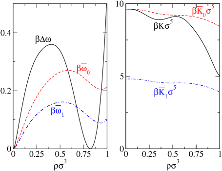
Figure 1: The free energy and SGA coefficient and their zeroth and first-order density moments for a Lennard-Jones fluid with no cutoff at $k_{B}T=0.75\epsilon=0.58k_{B}T_{c}$ and $\mu=\mu_{coex}$.

Figure 1 shows the free energy, density-averaged free energy and its first moment, $\Delta\omega\left(\rho,\rho_{v}\right),\bar{\omega}_{0}\left(\rho,\rho_{v}\right)$ and $\bar{\omega}_{1}\left(\rho,\rho_{v}\right)$, for the Lennard-Jones potential with no cutoff for coexistence, $\mu=\mu_{coex}$ and at temperature $k_{B}T=0.75\epsilon=0.58k_{B}T_{c}$ which is just above the triple point (and where $T_{c}=1.3\epsilon$ is the critical temperature). Also shown are $K\left(\rho\right)$, $\bar{K}_{0}\left(\rho,\rho_{v}\right)$ and $\bar{K}_{1}\left(\rho,\rho_{v}\right)$. The free energy, $\Delta\omega\left(\rho,\rho_{v}\right)$, has two minima corresponding to the vapor and the liquid states separated by a barrier of about $\allowbreak 0.36k_{B}T$. The density-averaged free energy shows less variation and the first moment is about half as large. The SGA coefficient varies relatively little as a function of density thus showing that it is dominated by the density-independent potential contributions. As a consequence, the density-averaged value is nearly constant and the first moment is very nearly half as large, $\bar{K}_{1}\left(\rho,\rho_{v}\right)\simeq\frac{1}{2}\bar{K}_{0}\left(\rho,\rho_{v}\right)$, over the whole range of densities. In Fig.2, the same quantities are shown for $k_{B}T=1.2\epsilon=0.92k_{B}T_{c}$. In this case, the difference between the free energy moments is much less but the SGA coefficient is still dominated by the density-independent contributions.

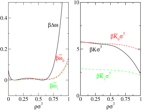
Figure 2: The same as Fig.1 but for $k_{B}T=1.2\epsilon=0.92k_{B}T_{c}$.

IV.1 Planar interface

As a first test of the SGA, the profile and excess free energy of the planar liquid-vapor interface at coexistence was calculated for the Lennard-Jones potential truncated at various positions, $r_{c}$, and shifted so that $v(r_{c})=0$. Figure 3 shows the excess free energy per unit area, or surface tension, as a function of temperature from the calculations as well as that calculated in the piecewise linear model and values obtained from Monte Carlo simulationsPGLutsko . The accuracy of the calculations is evident. In fact, the accuracy of the SGA appears to rival that of the underlying DFT (see Ref.Lutsko_JCP_2008 for comparison). The piecewise-linear approximation always gives higher values of the surface tension, as it must since the SGA result is obtained via an unconstrained minimization of the free energy, but is nevertheless very close to the SGA result.

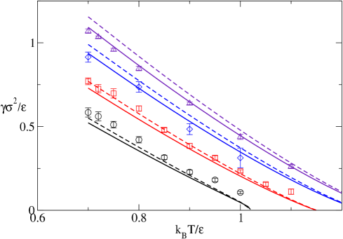
Figure 3: The surface tension as a function of temperature for potentials cutoff at $r_{c}=6\sigma$ (upper curves and symbols), $r_{c}=4\sigma$, $r_{c}=3\sigma$ and $r_{c}=2.5\sigma$ (lower curves and symbols). The symbols are the simulation data and error bars reported in Ref.PGLutsko , the full lines are from the SGA calculations and the dashed lines are from the piecewise-linear model.

Some calculated profiles are shown in Fig.4 and compared to simulation data reported in Ref.PGLutsko . The SGA profiles are in reasonable agreement with the simulations although some discrepancy is apparent, particularly in the narrowest interfaces. The crudeness of the piecewise-linear approximation is apparent; even so, the widths of the interfaces are tracked reasonably well as a function of cutoff and temperature.

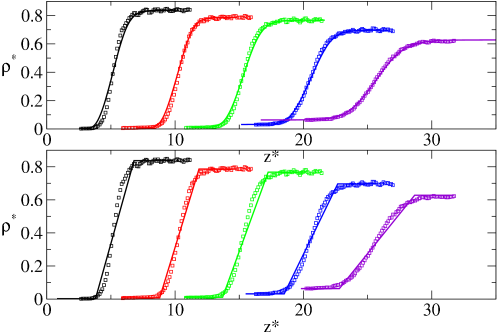
Figure 4: (Color online) Density profiles at the liquid-vapor interface calculated at different temperatures and values of the potential cutoff. From left to right, the curves correspond to $k_{B}T/\epsilon\equiv T^{*}=0.7$ and $r_{c}^{*}=5.0$, $T^{*}=0.7$ and $r_{c}^{*}=2.5$, $T^{*}=0.8$ and $r_{c}^{*}=5.0$, $T^{*}=0.8$ and $r_{c}^{*}=2.5$ and $T^{*}=1.1$ and $r_{c}^{*}=5.0$. The upper panel shows curves calculated in the SGA while the lower one shows the piece-wise linear approximation. The symbols are the data reported in ref. Mecke-LJ_Interface and extracted from ref. Katsov as the original is no longer availableFisher .

To illustrate the convergence to the exact result as the number of links in the profile increases, calculations were performed while varying the number of links. The results are shown in Fig.5 which shows that the simple single-link profile gives an error of about $5\%$ and that this decreases to about $0.5\%$ for 10 links. Linear extrapolation of the values as a function of $1/N$ gives the exact value.

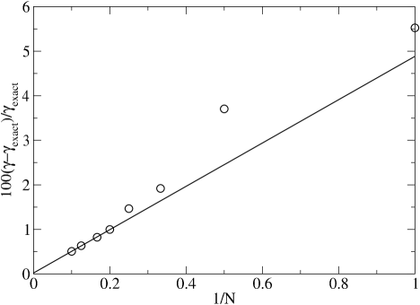
Figure 5: The relative error in the surface tension as calculated using piecewise-linear profiles with varying numbers of links, $N$, for $r_{c}^{*}=6$ and for $T^{*}=0.7$. The line shows the linear extrapolation of the profiles with 5,6,8 and 10 links demonstrating convergence to the exact value.

IV.2 Clusters

Small clusters pose more of a challenge since there is no bulk region and most, if not all, of the atoms in the cluster are affected by the interface. Furthermore, all clusters are out of equilibrium except the critical cluster which is in a metastable state. The description of unstable clusters will be discussed below: here attention is focussed on the transition states: i.e., the critical clusters.

Using the SGA, the properties of critical clusters were determined by solving Eq.(7) in a spherically symmetric geometry using a relaxation techniqueNR . Given an initial guess of the profile not too different from the critical cluster, this method relaxes to the critical cluster automatically. For the analytic model, the eigenvalue-following technique described above was used. The protocol is the same as described in Ref.Lutsko_JCP_2008_2 including a small temperature correction to account for deficiencies in the equation of state for small cutoffs.

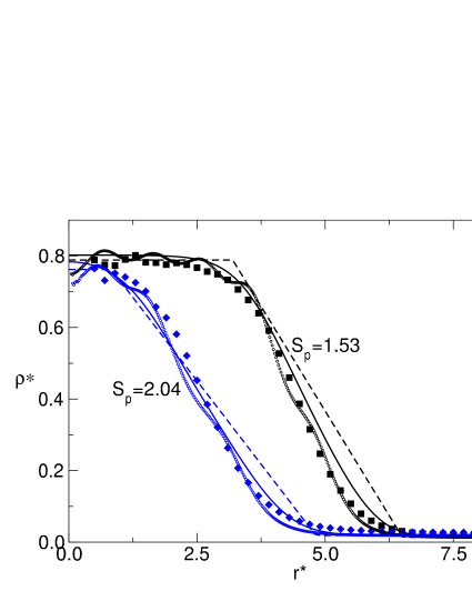
Figure 6: (Color online) Density profiles of the critical cluster for two different values of the supersaturation for the Lennard-Jones potential with cutoff $r_{c}=2.5\sigma$ and $k_{B}T/\epsilon=0.741$. The full symbols are the simulation data from Ref. frenkel_gas_liquid_nucleation , the full lines were calculated using the SGA, the dashed lines are the piecewise-analytic approximation and the open circles are the result of the full MC-VDWLutsko_JCP_2008_2 .

Figure 6 shows the density profiles for critical clusters at two different values of the supersaturation as well as simulation data from ten Wolde and Frenkelfrenkel_gas_liquid_nucleation . Note that following Ref.frenkel_gas_liquid_nucleation , supersaturation is defined as the ratio of the vapor pressure to that at coexistence. The SGA is seen to give a good description of the critical clusters, although there are greater differences from simulation than in the case of the planar profiles. In particular, the SGA profiles have wider interfaces than occurs in the data and the larger profile, corresponding to lower supersaturation, has somewhat larger radius than indicated by simulation. Also shown are the analytic approximations which give a reasonable approximation to the SGA profiles but which are still wider and therefore compare less well to simulation. To put these results in context, the underlying MC-VDW DFT model on which the present SGA is based is in close agreement with the simulated cluster profilesLutsko_JCP_2008_2 .

Figure 7 shows the cluster size and excess free energy as a function of supersaturation as computed from the SGA, the piecewise-linear profiles, CNT and determined from simulation. The SGA gives a good estimate of the free energy barrier, but systematically underestimates the cluster size due to more rapid convergence to the bulk vapor density. The analytic profiles again give reasonable approximations to the SGA. As noted by ten Wolde and Frenkelfrenkel_gas_liquid_nucleation CNT gives good estimates of the cluster size and poorer estimates for the barrier, especially at higher supersaturations.

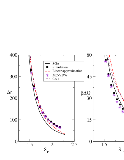
Figure 7: (Color online) The properties of the critical cluster as a function of supersaturation for the Lennard-Jones potential with cutoff $r_{c}=2.5\sigma$ and $k_{B}T/\epsilon=0.741$. The panel on the left shows the excess number of atoms in the cluster and that on the right shows the excess free energy. The squares are the simulation data from Ref. frenkel_gas_liquid_nucleation , the full lines are the result of solving the SGA, Eq.(19), the dashed-lines are from the piecewise-linear approximation and, for comparison, the results obtained from the full MC-VDW DFTLutsko_JCP_2008_2 are shown as stars and the CNT result is shown as a dashed-dotted line.

IV.3 Nucleation Pathways

The steepest descent pathways have been calculated by integrating Eq.(50) for several values of the supersaturation. Figure 8 shows the excess number of atoms in a cluster as a function of the distance along the pathway for two cases showing that $\Delta N$ is a monotonic function of the distance and therefore could serve as a reaction coordinate. Figure 9 illustrates the actual pathways and shows some surprising features. Although the excess number of atoms is a monotonic function of the path, the size of the bulk region, parameterized by $R$, and the width of the interface, parameterized by $w$, are both non-monotonic functions along the steepest-descent pathway. The width in particular grows with growing droplet size for small droplets until it reaches a maximum for clusters of about $75$ atoms and then slowly decreases thereafter. The size of the bulk region shows a local minimum at about the same point as the width has a maximum and is a decreasing function of cluster size for small clusters of $30-75$ atoms.

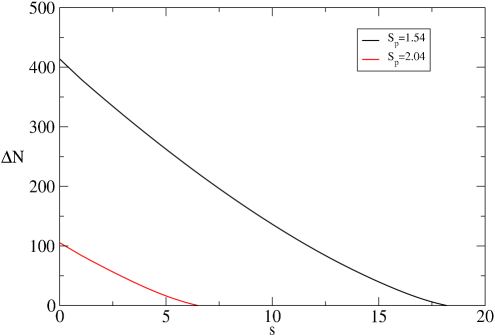
Figure 8: (Color online) The excess number of atoms in a cluster as a function of distance along the steepest-descent paths where $s=0$ corresponds to the critical cluster. The figure shows the results for the Lennard-Jones potential with a cutoff at $2.5\sigma$ for $T=0.683T_{c}$ for two different values of the supersaturation and illustrates the fact that the excess number varies monotonically with distance along the path so that it can sensibly be used as a reaction coordinate.

Figure 9 also shows the minimum energy pathways obtained by minimizing with respect to all parameters while holding $\Delta N$ fixed. The fact, noted above, that the inner density is incorrect for large $\Delta N$ is evident. However, the critical clusters are accurately determined since they are stationary points with respect to all parameters. This means that any energy minimized path, regardless of the constraints, will give the correct critical cluster. For smaller clusters, the fixed-$\Delta N$ paths are in qualitative agreement with the steepest descent paths showing the same non-monotonic behavior of both the width and radius. However, rather than varying smoothly and continuously as the cluster size goes to zero, it was found that below a certain cluster size, the energy-minimized path jumped discontinuously to a solution consisting of a very low central density, only slightly larger than the gas, and a very large width. This is not an accident: for the small values of $\Delta N$, there are no energy-minimized clusters with liquid-like cores. Calculations of the energy-minimized path at fixed equimolar radius gave good agreement with the steepest-descent paths for large clusters, but show similar unphysical behavior (i.e. the absence of liquid-like cores) beginning at larger cluster sizes than for the fixed $\Delta N$ paths. The conclusion is that while energy-minimized paths can give qualitative behavior similar to the steepest descent paths, they do not give a reasonable physical description of the entire nucleation pathway. This is somewhat at odds with the recent results of Ghosh and GhoshGhosh who examine energy-minimized paths at fixed radius for sigmoidal profiles and who appear to obtain nontrivial minimizations at all values of the radius. Perhaps this is simply due the use of different equations of state and values of the squared-gradient coefficient or because the piece-wise linear model is too crude. Another possibility is that it is related to the fact that the sigmoidal profile does not enforce the boundary condition that $d\rho(r)/dr=0$ at $r=0$ as do the piecewise-linear profiles used here and so are less constrained. Note that this boundary condition is used when solving the SGA Euler-Lagrange equations, Eq.(19), for the critical cluster and that without it, derivatives such as $d\rho(x,0,0)/dx$ do not exist at $x=0$.

Another interesting feature of the steepest-descent pathways is that the the interior density is that of the metastable vapor for very small clusters and increases rapidly as a function of cluster size until the cluster reaches about $100$ atoms. Since the radius of the bulk region never fully goes to zero, this gives a very different picture of the formation of small clusters from that implied in CNT. Recall that in the CNT model, small clusters have small radii while the central density is always that of the bulk. Here, the picture is one of increasing density in a bulk region that is always of finite extent. Figure 10 shows the equimolar radius which further emphasizes this difference. Whereas in the CNT model, the equimolar radius is equal to the radius of the cluster, and therefore goes to zero for small clusters, here it is a function of both the radius of the bulk region and the width and in fact is never small than about $2\sigma$. This is very similar to results found using the NEB method and a much more sophisticated DFT modelLutskoBubble1 ; Lutsko_JCP_2008_2 . Here, however, the physics behind this behavior is evident. As shown above, the surface free energy is proportional to the difference in densities inside and outside the droplet and inversely proportional to the width of the interfacial region. In order to minimize the free energy for small droplets, which is dominated by the surface tension contribution, as the size of the droplets decreases, the difference in densities must decrease as well. Since the free energy is inversely proportional to the width, the width stabilizes at a finite value and the $\Delta N\rightarrow 0$ limit is achieved via $\rho_{0}\rightarrow\rho_{\infty}$ at finite $w$ giving a non-zero equimolar radius.

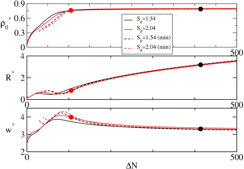
Figure 9: (Color online) The inner density, $\rho_{0}$, the radius, $R$, and the width, $w$, as a function of excess number of atoms in a cluster for the same conditions as described in Fig. 8. The full curves are the result of solving the steepest descent equations and the symbols mark the critical clusters. The dashed lines are the minimum-energy pathways calculated for fixed $\Delta N$.

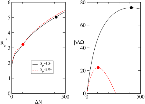
Figure 10: (Color online) The equimolar radius (left panel) and the excess free energy (right panel) as a function of cluster size as calculated along the steepest descent paths. The calculations were performed for two values of the supersaturation and the critical cluster in each case is indicated with a circle.

V Conclusions

The construction of the Squared-Gradient approximation starting with the Modified-Core van der Waals model for inhomogeneous fluids has been described. A relatively simple expression for the SGA coefficient was obtained which requires only the equation of state and interaction potential as input. The SGA model was shown to give quantitatively accurate surface free energies and density profiles for planar liquid-vapor interfaces of Lennard-Jones fluids as a function of temperature and potential cutoff. Similar comparisons were made for spherical clusters where it was found that the SGA was less accurate than the full DFT model nevertheless gives reasonable results.

It was also shown that the SGA could further be approximated using piecewise-linear density profiles. This model is of course less accurate in the same examples (planar interfaces and spherical clusters) than the SGA but is not unreasonable given its simplicity. Aside from providing a rather simple means to explore the solution of the SGA, the main advantage of the piecewise-linear model is that it offers a simple bridge between DFT and the ideas behind Classical Nucleation Theory.

Finally, the use of these tools to construct a description of homogeneous liquid-vapor nucleation was illustrated. The description was based on an analogy to chemical and structural transitions and made use of the transition-state/steepest-descent path methods used in those problems. Interesting non-classical behavior that was observed included the decrease of the interior density and the finite equimolar-radius as the size of the clusters tended to zero. Both effects were linked to the fact that the effective surface tension is density-dependent (unlike in CNT), a fact that is immediately evident in the case of the piecewise-linear approximation but that would be harder to isolate in purely numerical calculations using the SGA or the original DFT. This density dependence is crucial in following small clusters as, otherwise, the surface tension would cause $\Delta\Omega$ to diverge as the interfacial width goes to zero. This serves to illustrate the utility of such simple, yet not unrealistic, approximate methods in developing physical understanding of the more complex calculations.

Appendix A Evaluation of the coefficients

From Eq.(13), the explicit expression for the core-correction coefficients is

$$b_{0} =\frac{3}{\pi d^{3}}\left(\frac{\partial^{2}}{\partial\overline{\rho}^{2}}f_{HS}\left(\overline{\rho}\right)-\frac{\partial^{2}}{\partial\overline{\rho}^{2}}f\left(\overline{\rho}\right)\right)+3c_{HS}\left(d_{-};\overline{\rho},d\right)+3\beta v\left(d\right)+\frac{12}{d^{3}}\int_{d}^{\infty}\beta v\left(r\right)r^{2}dr$$ (52)

$$b_{1} =-\beta v\left(d\right)-c_{HS}\left(d_{-};\overline{\rho},d\right)-b_{0}$$

The gradient theory coefficient is given by

$$K = \frac{4\pi}{6}\int_{0}^{\infty}c_{HS}\left(r;\overline{\rho};d\right)r^{4}dr+\frac{4\pi}{6}\int_{0}^{d}\left(b_{0}+b_{1}\frac{r}{d}\right)r^{4}dr-\frac{4\pi}{6}\int_{d}^{\infty}\beta v\left(r\right)r^{4}dr$$

$$= \frac{4\pi}{6}\int_{0}^{\infty}c_{HS}\left(r;\overline{\rho};d\right)r^{4}dr+\frac{\pi d^{5}}{45}\left(6b_{0}+5b_{1}\right)-\frac{4\pi}{6}\int_{d}^{\infty}\beta v\left(r\right)r^{4}dr$$

$$= \frac{4\pi}{6}\int_{0}^{\infty}c_{HS}\left(r;\overline{\rho};d\right)r^{4}dr+\frac{\pi d^{5}}{9}\left(-\beta v\left(d\right)-c_{HS}\left(d_{-};\overline{\rho},d\right)\right)+\frac{\pi d^{5}}{45}b_{0}-\frac{4\pi}{6}\int_{d}^{\infty}\beta v\left(r\right)r^{4}dr$$

$$= \frac{4\pi}{6}\int_{0}^{\infty}c_{HS}\left(r;\overline{\rho};d\right)r^{4}dr-\frac{2}{45}\pi d^{5}c_{HS}\left(d_{-};\overline{\rho},d\right)+\frac{\pi d^{5}}{45}\left(\frac{3}{\pi d^{3}}\left(\frac{\partial^{2}}{\partial\overline{\rho}^{2}}f_{HS}\left(\overline{\rho}\right)-\frac{\partial^{2}}{\partial\overline{\rho}^{2}}f\left(\overline{\rho}\right)\right)\right)$$

$$-\frac{2}{45}\pi d^{5}\beta v\left(d\right)+\frac{4\pi}{30}\int_{d}^{\infty}\left(2d^{2}-5r^{2}\right)\beta v\left(r\right)r^{2}dr$$

Then, using

$$\frac{\partial^{2}}{\partial\overline{\rho}^{2}}\left(\beta f_{HS}\left(\overline{\rho}\right)-\beta f_{id}\left(\overline{\rho}\right)\right)=-\int c_{HS}\left(r;\overline{\rho};d\right)d\mathbf{r}$$ (54)

gives

$$K = \frac{4\pi}{30}\int_{0}^{\infty}c_{HS}\left(r;\overline{\rho};d\right)\left(5r^{2}-2d^{2}\right)r^{2}dr-\frac{2}{45}\pi d^{5}c_{HS}\left(d_{-};\overline{\rho},d\right)-\frac{d^{2}}{15}\frac{\partial^{2}}{\partial\overline{\rho}^{2}}f_{ex}\left(\overline{\rho}\right)$$

$$- \frac{2}{45}\pi d^{5}\beta v\left(d\right)+\frac{4\pi}{30}\int_{d}^{\infty}\left(2d^{2}-5r^{2}\right)\beta v\left(r\right)r^{2}dr$$

For both the Percus-Yevick approximation and the more accurate White-Bear DFT, the hard-sphere DCF can be written as

$$c_{HS}\left(r;\overline{\rho};d\right)=\left(a_{0}+a_{1}\frac{r}{d}+a_{3}\left(\frac{r}{d}\right)^{3}\right)\Theta\left(d-r\right)$$ (56)

giving

$$\beta K\left(\bar{\rho}\right) = -\frac{\pi d^{5}}{180}a_{3}\left(\overline{\rho}d^{3}\right)-\frac{d^{2}}{15}\frac{\partial^{2}}{\partial\overline{\rho}^{2}}\beta f_{ex}\left(\overline{\rho}\right)-\frac{2\pi}{45}d^{5}\beta v\left(d\right)+\frac{2\pi}{15}\int_{d}^{\infty}\left(2d^{2}-5r^{2}\right)\beta v\left(r\right)r^{2}dr$$

$$= -\frac{\pi d^{5}}{180}a_{3}\left(\overline{\rho}d^{3}\right)-\frac{d^{2}}{15}\frac{\partial^{2}}{\partial\overline{\rho}^{2}}\beta f_{ex}\left(\overline{\rho}\right)+\frac{2\pi}{45}\int_{d}^{\infty}\left(3r^{5}-2d^{2}r^{3}\right)\frac{d\beta v\left(r\right)}{dr}dr$$

Finally,

$$\left.\frac{\partial^{2}}{\partial\overline{\rho}^{2}}f\left(\overline{\rho}\right)\right|_{V,T} = \left.\frac{\partial\mu}{\partial\overline{\rho}}\right|_{V,T}$$

$$= \left.\frac{\partial\left(\frac{f}{\overline{\rho}}+\frac{\beta P}{\overline{\rho}}\right)}{\partial\overline{\rho}}\right|_{V,T}$$

$$= \overline{\rho}^{-1}\left.\frac{\partial f}{\partial\overline{\rho}}\right|_{V,T}-\frac{f}{\overline{\rho}^{2}}+\overline{\rho}^{-1}\left.\frac{\beta P}{\partial\overline{\rho}}\right|_{V,T}-\frac{\beta P}{\overline{\rho}^{2}}$$

$$= \overline{\rho}^{-1}\left.\frac{\beta P}{\partial\overline{\rho}}\right|_{V,T}$$

$$= \overline{\rho}^{-2}\kappa_{T}$$

where the isothermal compressibility is

$$\kappa_{T}=\beta_{T}^{-1}=-V\frac{\partial\beta P}{\partial V}$$ (59)

So

$$K=-\frac{\pi d^{5}}{180}a_{3}-\frac{d^{2}}{15}\overline{\rho}^{-2}\kappa_{T}-\frac{2\pi}{45}d^{5}\beta v\left(d\right)+\frac{2\pi}{45}\int_{d}^{\infty}\left(3r^{5}-2d^{2}r^{3}\right)\frac{d\beta v\left(r\right)}{dr}dr$$ (60)

For packing fraction $\eta=\frac{\pi}{6}\rho d^{3}$, the Percus-Yevick approximation gives

$$a_{3}=-\frac{\eta}{2}\frac{\left(1+2\eta\right)^{2}}{\left(1-\eta\right)^{4}}$$ (61)

while in the White-Bear approximation,

$$a_{3}=\frac{-3+10\eta-15\eta^{2}+5\eta^{3}}{\left(1-\eta\right)^{4}}-\frac{3\ln\left(1-\eta\right)}{\eta}$$ (62)

Appendix B More general planar interfaces

The piecewise-linear model is easily extended to include an arbitrary number of pieces. The density profile becomes

$$\rho\left(z\right)=\left\{\begin{array}[]{c}\rho_{-\infty},\;z<0\\ \rho_{-\infty}+\left(\rho_{1}-\rho_{-\infty}\right)\frac{z}{w_{1}},\;0<z<w_{1}\\ \rho_{1}+\left(\rho_{2}-\rho_{1}\right)\frac{z-w_{1}}{w_{2}},\;w_{1}<z<w_{1}+w_{2}\\ \rho_{2}+\left(\rho_{3}-\rho_{2}\right)\frac{z-w_{1}-w_{2}}{w_{3}},\;w_{1}+w_{2}<z<w_{1}+w_{2}+w_{3}\\ ...\\ \rho_{\infty},\;w_{1}+w_{2}+...+w_{n}<z\end{array}\right.$$

Defining

$$z_{i}=\sum_{j=1}^{i}w_{j}$$

this can be written as

$$\rho\left(z\right)=\left\{\begin{array}[]{c}\rho_{-\infty},\;z<0\\ \rho_{i-1}+\left(\rho_{i}-\rho_{i-1}\right)\frac{z-z_{i-1}}{w_{i}},\;z_{i-1}<z<z_{i}\\ \rho_{\infty},\;z_{n}<z\end{array}\right.$$ (63)

with the identifications $\rho_{0}=\rho_{-\infty}$, $\rho_{n}=\rho_{\infty}$. The free parameters are $\rho_{i}$ for $1\leq i\leq n-1$ and $w_{i}$ for $1\leq i\leq n$ giving a total of $2n-1$ parameters. Then, the excess energy is

$$\gamma = \frac{\Omega-\Omega_{coex}}{V}=\sum_{i=1}^{n}\int_{z_{i-1}}^{z_{i-1}+w_{i}}\left\{\omega\left(\rho\left(z\right)\right)-\omega_{coex}+\frac{1}{2}K\left(\rho\left(z\right)\right)\left(\frac{\rho_{i}-\rho_{i-1}}{w_{i}}\right)^{2}\right\}dz$$

$$= \sum_{i=1}^{n}\left\{w_{i}\int_{\rho_{i-1}}^{\rho_{i}}\left(\omega\left(x\right)-\omega_{coex}\right)dx+\frac{\left(\rho_{i}-\rho_{i-1}\right)^{2}}{2w_{i}}\int_{\rho_{i-1}}^{\rho_{i}}K\left(x\right)dx\right\}$$

which is simply the sum of the contribution of each link in the profile.

Appendix C Perturbative Solution for the spherical profile at constant particle number

The free energy is

$$\Delta\Omega=\frac{4\pi}{3}R^{3}\Delta\omega+4\pi R^{2}w\left(\overline{\omega}_{0}+2\overline{\omega}_{1}\left(\frac{w}{R}\right)+\overline{\omega}_{2}\left(\frac{w}{R}\right)^{2}+\frac{\left(\rho_{\infty}-\rho_{0}\right)^{2}}{2w^{2}}\left(\overline{K}_{0}+2\overline{K}_{1}\left(\frac{w}{R}\right)+\overline{K}_{2}\left(\frac{w}{R}\right)^{2}\right)\right)$$ (65)

which is to be minimized at constant particle number,

$$N=\int\left(\rho\left(\mathbf{r}\right)-\rho_{\infty}\right)d\mathbf{r}=\frac{\pi}{3}\left(\rho_{0}-\rho_{\infty}\right)\left(2R+w\right)\left(2Rw+2R^{2}+w^{2}\right)$$ (66)

Introducing a Lagrange multiplier,$\lambda$, and setting

$$0=\frac{\partial}{\partial\Gamma}\left(\Delta\Omega\left(R,\rho_{0},w\right)-\lambda\left(N-\frac{\pi}{3}\left(\rho_{0}-\rho_{\infty}\right)\left(2R+w\right)\left(2Rw+2R^{2}+w^{2}\right)\right)\right)$$

for $\Gamma=R,\rho_{0},w$ and $\lambda$ gives, after some simplification,

$$0 = \Delta\omega+2\frac{w}{R}\left(\overline{\omega}_{0}+\overline{\omega}_{1}\left(\frac{w}{R}\right)+\frac{\left(\rho_{0}-\rho_{\infty}\right)^{2}}{2w^{2}}\left(\overline{K}_{0}+\overline{K}_{1}\left(\frac{w}{R}\right)\right)\right)$$

$$+\lambda\frac{1}{3}\left(\rho_{0}-\rho_{\infty}\right)\left(3+3\left(\frac{w}{R}\right)+\left(\frac{w}{R}\right)^{2}\right)$$

$$0 = \frac{1}{3}\frac{\partial\Delta\omega}{\partial\rho_{0}}+\frac{w}{R}\left(\frac{\partial\overline{\omega}_{0}}{\partial\rho_{0}}+2\frac{\partial\overline{\omega}_{1}}{\partial\rho_{0}}\left(\frac{w}{R}\right)+\frac{\partial\overline{\omega}_{2}}{\partial\rho_{0}}\left(\frac{w}{R}\right)^{2}\right)$$

$$+\frac{w}{R}\frac{\left(\rho_{0}-\rho_{\infty}\right)^{2}}{2w^{2}}\left(\frac{\partial\overline{K}_{0}}{\partial\rho_{0}}+2\frac{\partial\overline{K}_{1}}{\partial\rho_{0}}\left(\frac{w}{R}\right)+\frac{\partial\overline{K}_{2}}{\partial\rho_{0}}\left(\frac{w}{R}\right)^{2}\right)$$

$$+\frac{w}{R}\frac{\left(\rho_{0}-\rho_{\infty}\right)}{w^{2}}\left(\overline{K}_{0}+2\overline{K}_{1}\left(\frac{w}{R}\right)+\overline{K}_{2}\left(\frac{w}{R}\right)^{2}\right)+\lambda\frac{1}{12}\left(4+6\frac{w}{R}+4\left(\frac{w}{R}\right)^{2}+\left(\frac{w}{R}\right)^{3}\right)$$

$$0 = \left(\overline{\omega}_{0}+4\overline{\omega}_{1}\left(\frac{w}{R}\right)+3\overline{\omega}_{2}\left(\frac{w}{R}\right)^{2}+\frac{\left(\rho_{0}-\rho_{\infty}\right)^{2}}{2w^{2}}\left(-\overline{K}_{0}+\overline{K}_{2}\left(\frac{w}{R}\right)^{2}\right)\right)$$

$$+\lambda\frac{1}{12}\left(\rho_{0}-\rho_{\infty}\right)\left(6+8\left(\frac{w}{R}\right)+3\left(\frac{w}{R}\right)^{2}\right)$$

$$0 = N-\frac{\pi}{3}\left(\rho_{0}-\rho_{\infty}\right)R^{3}\left(4+6\left(\frac{w}{R}\right)+4\left(\frac{w}{R}\right)^{2}+\left(\frac{w}{R}\right)^{3}\right)$$

These are solved perturbatively using $\epsilon\equiv N^{-1/3}$ as a small parameter where the expansion of the various quantities is assumed to take the form

$$R = \epsilon^{-1}R_{0}+R_{1}+\epsilon R_{2}+...$$ (68)

$$\rho_{0} = \rho_{00}+\epsilon\rho_{01}+...$$

$$w = w_{0}+\epsilon w_{1}+...$$

$$\lambda = \lambda_{0}+\epsilon\lambda_{1}+...$$

Then, the lowest order equations are

$$0 = \omega\left(\rho_{00}\right)-\omega\left(\rho_{\infty}\right)+\lambda_{0}\left(\rho_{00}-\rho_{\infty}\right)$$ (69)

$$0 = \frac{\partial\omega\left(\rho_{00}\right)}{\partial\rho_{00}}+\lambda_{0}$$

$$0 = \overline{\omega}_{0}\left(\rho_{\infty},\rho_{00}\right)-\frac{\left(\rho_{\infty}-\rho_{00}\right)^{2}}{2w_{0}^{2}}\overline{K}_{0}\left(\rho_{\infty},\rho_{00}\right)+\lambda_{0}\frac{1}{2}\left(\rho_{00}-\rho_{\infty}\right)$$

$$0 = 1-\frac{4\pi}{3}\left(\rho_{00}-\rho_{\infty}\right)R_{0}^{3}$$

giving

$$\lambda_{0} = -\frac{\omega\left(\rho_{00}\right)-\omega\left(\rho_{\infty}\right)}{\rho_{00}-\rho_{\infty}}$$ (70)

$$\frac{\partial\omega\left(\rho_{00}\right)}{\partial\rho_{00}} = \frac{\omega\left(\rho_{00}\right)-\omega\left(\rho_{\infty}\right)}{\rho_{00}-\rho_{\infty}}$$

$$w_{0}^{2} = \frac{\left(\rho_{\infty}-\rho_{00}\right)^{2}}{2\overline{\omega}_{0}\left(\rho_{\infty},\rho_{00}\right)-\left(\omega\left(\rho_{00}\right)-\omega\left(\rho_{\infty}\right)\right)}\overline{K}_{0}$$

$$R_{0}^{3} = \frac{3}{4\pi\left(\rho_{00}-\rho_{\infty}\right)}$$

Notice that the second equation can be written as

$$\frac{\partial f\left(\rho_{00}\right)}{\partial\rho_{00}}=\mu-\lambda_{0}$$ (71)

thus showing the shift of the chemical potential arising from the constraint.

Appendix D Metric

The metric is calculated using Eq.(49). The result for a piecewise-linear profile with a single link is

$$g_{\rho\rho} = \frac{2\pi}{15}\left(10R^{3}+10R^{2}w+5Rw^{2}+w^{3}\right)$$ (72)

$$g_{\rho R} = \left(\rho_{0}-\rho_{\infty}\right)\frac{\pi}{3}\left(6R^{2}+4Rw+w^{2}\right)$$

$$g_{\rho w} = \left(\rho_{0}-\rho_{\infty}\right)\frac{\pi}{15}\left(10R^{2}+10Rw+3w^{2}\right)$$

$$g_{RR} = \left(\rho_{0}-\rho_{\infty}\right)^{2}\frac{4\pi}{3}\frac{3R^{2}+3Rw+w^{2}}{w}$$

$$g_{Rw} = \left(\rho_{0}-\rho_{\infty}\right)^{2}\frac{\pi}{3}\frac{6R^{2}+8Rw+3w^{2}}{w}$$

$$g_{ww} = \left(\rho_{0}-\rho_{\infty}\right)^{2}\frac{2\pi}{15}\frac{10R^{2}+15Rw+6w^{2}}{w}$$

References

• (1) J. F. Lutsko, J. Chem. Phys. 128, 184711 (2008)
• (2) J. F. Lutsko, J. Laidet, and P. Grosfils, J. Phys.: Cond. Matt. 22, 035101 (2010)
• (3) J. F. Lutsko, J. Chem. Phys. 129, 244501 (2008)
• (4) J. S. Rowlinson, J. Stat. Phys. 20, 197 (1979)
• (5) J. D. van der Waals, Z. Phys. Chem. 13, 657 (1894)
• (6) V. Ginzburg and L. Landau, Zh. Eksp. Teor. Fiz. 20, 1064 (1950)
• (7) J. W. Cahn and J. E. Hilliard, J. Chem. Phys. 28, 258 (1958)
• (8) R. Evans, Adv. Phys. 28, 143 (1979)
• (9) H. Löwen, T. Beier, and H. Wagner, Europhys. Lett. 9, 791 (1989)
• (10) H. Löwen, T. Beier, and H. Wagner, Z. Phys. B 79, 109 (1990)
• (11) J. F. Lutsko, Physica A 366, 229 (2006)
• (12) P. M. W. Cornelisse, C. J. Peters, and J. de Swaan Arons, J. Chem. Phys. 106, 9820 (1997)
• (13) D. Wales, Energy Landscapes (Cambridge University Press, Cambridge, 2003)
• (14) J.-P. Hansen and I. McDonald, Theory of Simple Liquids (Academic Press, San Diego, Ca, 1986)
• (15) R. Evans, in Fundamentals of Inhomogeneous Fluids, edited by D. Henderson (Marcel Dekker, New York, New York, 1992)
• (16) J. F. Lutsko, J. Chem. Phys. 127, 054701 (2007)
• (17) J. A. Barker and D. Henderson, J. Chem. Phys. 47, 4714 (1967)
• (18) M. M. T. da Gama and R. Evans, Mol. Phys. 38, 367 (1979)
• (19) S. Ghosh and S. K. Ghosh, J. Chem. Phys. 134, 024502 (2011)
• (20) D. Kashchiev, Nucleation : basic theory with applications (Butterworth-Heinemann, Oxford, 2000)
• (21) M. Heymann and E. V. Eijnden, Phys. Rev. Lett. 100 (2008)
• (22) J. C. Mauro, R. J. Loucks, and J. Balakrishnan, J. Phys. Chem. A 109, 9578 (2005)
• (23) H. Jonsson, G. Mills, and G. K. Schenter, Surface Science 324, 305 (February 1995)
• (24) G. Henkelman and H. Jónsson, J. Chem. Phys. 113, 9978 (2000)
• (25) G. Henkelman, B. P. Uberuaga, and H. Jónsson, J. Chem. Phys. 113, 9901 (2000)
• (26) E. Weinan, W. Ren, and E. V. Eijnden, J. Chem. Phys. 126 (2007)
• (27) J. F. Lutsko, Europhys. Lett. 83, 46007 (2008)
• (28) J. K. Johnson, J. A. Zollweg, and K. E. Gubbins, Mol. Phys. 78, 591 (1993)
• (29) P. Grosfils and J. F. Lutsko, J. Chem. Phys. 130, 054703 (2009)
• (30) M. Mecke, J. Winkelmann, and J. Fischer, J. Chem. Phys. 107, 9264 (1997)
• (31) K. Katsov and J. D. Weeks, J. Phys. Chem. B 106, 8429 (2002)
• (32) J. Fischer, private communication (2007)
• (33) W. H. Press, S. A. Teukolsky, W. T. Vetterling, and B. P. Flannery, Numerical Recipes in C (Claredon Press, Oxford, 1993)
• (34) P. Rien ten Wolde and D. Frenkel, J. Chem. Phys. 109, 9901 (1998)