Gorenstein-duality for one-dimensional almost complete intersections – with an application to non-isolated real singularities

Abstract

We give a generalization of the duality of a zero-dimensional complete intersection to the case of one-dimensional almost complete intersections, which results in a Gorenstein module $M=I/J$. In the real case the resulting pairing has a signature, which we show to be constant under flat deformations. In the special case of a non-isolated real hypersurface singularity $f$ with a one-dimensional critical locus, we relate the signature on the jacobian module $I/J_{f}$ to the Euler characteristic of the positive and negative Milnor fibre, generalising the result for isolated critical points. An application to real curves in ${\mathbb{P}}^{2}({\mathbb{R}})$ of even degree is given.

1 Introduction

The algebraic determination of the number of real roots of a polynomial has a long history going back at least to Descartes. Of particular relevance are the methods of Sylvester and Hermite that determine the number of real roots as the signature of an associated quadratic form. For a nice account of the classical approaches we refer to [We].

In a similar spirit, the celebrated theorem of Eisenbud-Levine [EL], and Khimshiashvilli [K] provides an algebraic method to determine the local degree of a finite map germ $F:({\mathbb{R}}^{n},0)\longrightarrow({\mathbb{R}}^{n},0)$ with component functions $f_{1},f_{2},\ldots,f_{n}\in P:={\mathbb{R}}[[x_{1},x_{2},\ldots,x_{n}]]$. One considers the local ${\mathbb{R}}$-algebra

$${\cal A}_{F}:=P/(f_{1},f_{2},\ldots,f_{n}),$$

which has finite dimension precisely when $f_{1},f_{2},\ldots,f_{n}$ form a regular sequence in $P$. Morever, in that case ${\cal A}_{F}$ is a Gorenstein ring: if we let

$$h:=\left|\begin{array}[]{ccc}\partial_{1}f_{1}&\ldots&\partial_{n}f_{1}\\ \vdots&&\vdots\\ \partial_{1}f_{n}&\ldots&\partial_{n}f_{n}\\ \end{array}\right|$$

and choose any linear form $\phi:{\cal M}\longrightarrow{\mathbb{R}}$ with $\phi(h)\neq 0$, then the pairing

$$B_{\phi}:{\cal A}_{F}\times{\cal A}_{F}\longrightarrow{\mathbb{R}},\;(a,b)\mapsto\phi(a\cdot b)$$

is non-degenerate.

Theorem 1.1

(Eisenbud-Levine [EL], Khimshiashvilli [K]) If $\phi(h)>0$ then

$$Signature(B_{\phi})=Degree(F,0)$$

The theorem is a result of key importance and has been the starting point of many subsequent works. We mention a few of the applications and generalisations.

Consider an isolated complete intersection curve $C=f^{-1}(0)$, where $f:({\mathbb{R}}^{n},0)\longrightarrow({\mathbb{R}}^{n-1},0)$. According to Aoki, Fukuda and Nishimura [AFN], one can compute the number of real branches of $C$ as follows: consider $g:=x_{1}^{2}+x_{2}^{2}+\ldots+x_{n}^{2}$ and let

$$Jac(g):=\left|\begin{array}[]{ccc}\partial_{1}g&\ldots&\partial_{n}g\\ \partial_{1}f_{1}&\ldots&\partial_{n}f_{1}\\ \vdots&&\vdots\\ \partial_{1}f_{n-1}&\ldots&\partial_{n}f_{n-1}\\ \end{array}\right|$$

On the ${\mathbb{R}}$-algebra ${\cal A}_{f,Jac(g)}:=P/(f_{1},\ldots,f_{n-1},Jac(g))$ one defines as above a pairing $B_{\phi}$.

Theorem 1.2

(Aoki-Fukuda-Nishimura)

$$Signature(B_{\phi})=\textup{Number of real branches of}\;\;C$$

This result was further generalised to the case of arbitrary Gorenstein curve singularities $C$ in [MvS].

In a similar vein, the work [Sz1] associates to a polynomial mapping $f:{\mathbb{R}}^{n}\longrightarrow{\mathbb{R}}^{k}$ an ${\mathbb{R}}$-algebra ${\cal A}$ with a quadratic form $B_{\phi}$ such that

$$Signature(B_{\phi})=\chi(f^{-1}(0)),$$

and further variations can be found in [Sz2], [Sz3], [D].

Another type of application is to the topology of real hypersurface singularities. A function $f\in P$ defines an isolated hypersurface singularity precisely when the partial derivatives $f_{i}:=\partial f/\partial x_{i}$ form a regular sequence in $P$. In this case the algebra ${\cal A}$ is nothing but the (real) Milnor algebra $P/J_{f}$, where $J_{f}$ is the jacobian ideal of $f$. The degree of $F:=(\partial_{1}f,\ldots,\partial_{n}f)$ is the Poincaré-Hopf index of the gradient vector field of $f$.

The Milnor ring is the most important algebraic invariant of the singularity $f$. Its dimension $\mu(f):=\dim(P/J_{f})$ is the Milnor number, which equals the dimension of the cohomology $H^{n-1}(F)$ of the Milnor fibre $F$, [AGV], [Mi]. In the real case one can also consider the real Milnor fibres:

$$F_{\epsilon,\eta}:=\{x\in{\mathbb{R}}^{n}\;|\;\|x\|\leq\epsilon,f(x)=\eta\},\;\;0<\epsilon\ll 1,\;\;0<\eta\ll\epsilon$$

For $\eta>0$, we put $F_{+}:=F_{\epsilon,\eta}$ and $F_{-}:=F_{\epsilon,-\eta}$ and call them the positive and negative Milnor fibers of $f$.

Theorem 1.3

([A]) Let $f\in{\mathbb{R}}\{x_{1},x_{2},\ldots,x_{n}\}$ have an isolated critical point at the origin. Then:

$$Signature(f)=-\widetilde{\chi}(F_{-})=(-1)^{n-1}\widetilde{\chi}(F_{+}),$$

where $\widetilde{\chi}$ denotes the reduced Euler characteristic.

Although the positive and negative Milnor fibre have, in general, a quite different topology, it is a simple but remarkable fact that their reduced Euler characteristics are the same, up to a sign. The real $D_{4}$ surface singularity defined by $x(x^{2}-y^{2})+z^{2}=0$ may exemplify this.

negative Milnor fibre	$D_{4}$ singularity	positive Milnor fibre

In this paper we give a partial generalisation of this result to the case where the sequence $f_{1},f_{2},\ldots,f_{n}$ defines a one-dimensional locus. In this case one says the the ideal $J=(f_{1},\ldots,f_{n})$ defines an almost complete intersection. We show that the torsion sub-module $M=I/J$ of $P/J$ is a Gorenstein module. An isomorphism $\phi:P\stackrel{{\scriptstyle\cong}}{{\longrightarrow}}\Omega^{n}_{P}$ determines a natural pairing

$$B_{\phi}:I/J\times I/J\longrightarrow{\mathbb{R}}$$

Its signature is an invariant of the real topology of the situation.

In the case of partial derivatives $f_{i}=\partial f/\partial x_{i}$ of a function $f$ with a one-dimensional critical locus, such modules $I/J_{f}$ were also considered by Ruud Pellikaan [P1] under the name of jacobian module. The case where $I$ is a radical ideal defining a reduced curve, corresponds to $f$ having transverse type $A_{1}$. We proof the following theorem

Theorem 1.4

Assume that $f\in{\mathbb{R}}\{x_{1},x_{2},\ldots,x_{n}\}$ has one-dimensional critical locus and transverse type $A_{1}$. Assume furthermore that either $f$ has a morsification or that $n=3$. Then

$$2Signature(B_{\phi})=-\widetilde{\chi}(F_{-})+(-1)^{n-1}\tilde{\chi}(F_{+})$$

wher as before $F_{\pm}$ are the positive and negative Milnor fibres of $f$ and $\widetilde{\chi}$ denotes the reduced Euler characteristic.

Note that contrary to case of isolated singularities, the two Euler characteristics appearing at the right hand side are in general no longer equal up to a sign. It appears that the above statement has a much broader range of validity, and holds for many other transverse types of singularities. However, as stated, it is not true in full generality, but we were not able to identify the precise limits of its validity.

A nice application arises in the situation of a homogeneous polynomial $f\in{\mathbb{R}}[x,y,z]$ of even degree. It defines a curve $C=\{f=0\}\subset{\mathbb{P}}^{2}({\mathbb{R}})$, whose complement consists of a part $V_{+}$ where $f>0$ and a part $V_{-}$ where $f<0$.

Theorem 1.5

If $f\in{\mathbb{R}}[x,y,z]$ defines a curve with only ordinary double points, then

$$Signature(B_{\phi}(f))=\chi(V_{+})-\chi(V_{-})$$

The structure of the paper is as follows. After reviewing the duality in the complete intersection case, we explain the emergence of the Gorenstein module $I/J$ for one-dimensional almost complete intersections and explain how the pairing behaves in a relative situation. Then we revies some material about singularities with one-dimensional singular locus that provide a rich source of examples and explain for special situations the meaning of the resulting signature in the real case,

2 Duality for zero-dimensional complete intersections

Let $P=K[[x_{1},x_{2},\ldots,x_{n}]]$ or any other regular local $K$-algebra of dimension $n$. Let there be given a sequence of elements

$$f_{1},\ldots,f_{n}\in P$$

and let $J$ be ideal generated by them. We denote the Koszul-complex associated to the sequence ${\bf f}:=f_{1},f_{2},\ldots,f_{n}$ by

$$K_{\bullet}({\bf f}):=0\rightarrow K_{n}\rightarrow K_{n-1}\rightarrow\cdots\rightarrow K_{2}\rightarrow K_{1}\rightarrow K_{0}\rightarrow 0$$

Its terms are $K_{p}:=\bigwedge^{p}P^{n}$, so that $K_{0}=P$. The differentials are induced by sending the $i$-th basis vector $e_{i}$ of $P^{n}$ to $f_{i}\in P$. We denote its homology groups by

$$H_{k}({\bf f}):=H_{k}(K_{\bullet}({\bf f}))$$

The following result is well-known (see e.g. [BH], thm. 1.6.17 and thm. 2.1.2).

Proposition 2.1

Let $V(J)\subset Spec(P)$ the variety defined by the ideal $J$ and let $d:=dim(V(J))$. Then $H_{k}({\bf f})=0$ for $k>d$ and $H_{d}({\bf f})\neq 0$

Let us first look at the case where $\dim(J)=0$. Then the above result tells us that $H_{0}({\bf f})=P/J$ and $H_{k}({\bf f})=0$ for $k>0$. So ${\bf f}$ is a regular sequence and the Koszul complex provides a free resolution of $P/J$ as a $P$-module. As the transpose of the map $K_{n}\longrightarrow K_{n-1}$ can be identified, up to signs, with the map $K_{1}\longrightarrow K_{0}$, we obtain an isomorphism

$$Ext^{n}_{P}(P/J,P)\cong P/J$$

Recall Grothendiecks local duality theorem (see e.g. [BH], thm. 3.5.8):

Theorem 2.2

Let $P$ be a $n$-dimensional local ring with maximal ideal ${\mathfrak{m}}$ and dualizing module $\omega_{P}$. For any finitely generated $P$-module $M$, there exists a natural non-degenerate pairing

$$H^{i}_{\mathfrak{m}}(M)\times Ext^{n-i}_{P}(M,\omega_{P})\longrightarrow H^{n}_{\mathfrak{m}}(\omega_{P})\stackrel{{\scriptstyle tr}}{{\longrightarrow}}K$$

In particular, for $M=P/J$ and $i=0$ we obtain a non-degenerate pairing

$$P/J\times Ext^{n}_{P}(P/J,\omega_{P})\longrightarrow K$$

as $H^{0}_{\mathfrak{m}}(P/J)=P/J$. The choice of an isomorphism $\phi:P\stackrel{{\scriptstyle\cong}}{{\longrightarrow}}\omega_{P}$ induces isomorphisms

$$Ext^{n}_{P}(P/J,\omega_{P})\cong Ext^{n}_{P}(P/J,P)\cong P/J$$

then hence provides us with a perfect pairing

$$B_{\phi}:P/J\times P/J\longrightarrow K$$

As $B_{\phi}$ is $P$-linear, it follows that it factors over the multiplication map and is of the form $B_{\phi}(a,b)=\beta(a\cdot b)$ for some linear form

$$\beta:P/J\longrightarrow K$$

The linear space $ker(\beta)$ is the socle of $P/J$, that is, its unique minimal ideal. There is a classical result of Scheja and Storch that states that this socle has a canonical generator.

Theorem 2.3

[SS] If $char(K)=0$ and $x_{1},\ldots,x_{n}$ are generators of the maximal ideal, then the Jacobian determinant

$$h:=\left|\begin{array}[]{ccc}\frac{\partial f_{1}}{\partial x_{1}}&\ldots&\frac{\partial f_{1}}{\partial x_{n}}\\ \vdots&&\vdots\\ \frac{\partial f_{n}}{\partial x_{1}}&\ldots&\frac{\partial f_{n}}{\partial x_{n}}\\ \end{array}\right|$$

is a generator for the socle of $P/J$.

Remark 2.4

In the case where $f\in P$ and $f_{i}=\partial f/\partial x_{i}$, the complex can be identified (up to some signs) with the $df\wedge$-complex

$$0\longrightarrow P\stackrel{{\scriptstyle df\wedge}}{{\longrightarrow}}\Omega^{1}\stackrel{{\scriptstyle df\wedge}}{{\longrightarrow}}\ldots\longrightarrow\Omega^{n-1}\stackrel{{\scriptstyle df\wedge}}{{\longrightarrow}}\Omega^{n}\longrightarrow 0$$

and the natural pairing takes the form

$$B:\Omega^{n}/df\wedge\Omega^{n-1}\times\;\;\Omega^{n}/df\wedge\Omega^{n-1}\longrightarrow K$$

It is usually called residue pairing and has an analytic expression as

$$B(P\omega,Q\omega)=\frac{1}{(2\pi i)^{n}}\int_{T_{\epsilon}}\frac{PQ\omega}{\partial_{1}f\ldots\partial_{n}f}$$

where $\omega:=dx_{1}\wedge dx_{2}\wedge\ldots\wedge dx_{n}$ and $T_{\epsilon}:=\{x\;|\;|\partial_{i}f|=\epsilon\}$, $0<\epsilon\ll 1$. In the papers [GV], [V] the relation between this pairing and the Poincaré-pairing in the cohomology of the Milnor fibre is described. The pairing is also the first in a sequence of higher residue pairings, introduced by K. Saito, which express the self-duality of the Gauß-Manin system of the singularity, [Sa].

3 Homology and Cohomology

We have seen that in the case of a regular sequence ${\bf f}$, the origin of the pairing on $P/J$ lies in the self-dual nature of the Koszul complex. We now investigate in general what consequence this self-duality has for the Koszul homology groups.

Proposition 3.1

(c.f. [E], prop. 17.15) Let ${\bf f}=f_{1},f_{2},\ldots,f_{n}$ be a sequence of elements in a ring $P$. There are isomorphisms

$$\alpha_{p}:H_{p}\left({\bf f}\right)\cong H^{n-p}\left({\bf f}\right),\;\;p=0,1,\ldots,n,$$

where $H^{p}({\bf f}):=H^{p}(Hom_{P}\left(K_{\bullet}\left({\bf f}\right),P\right))$ is the Koszul cohomology.

Proof.

Using the basis $e_{1},e_{2},\ldots,e_{n}$ for the free module $P^{n}$ and the dual basis $\phi_{1},\ldots,\phi_{n}$ for the dual module $Hom_{P}(P^{n},P)$, one obtains basis elements $e_{I}:=e_{i_{1}}\wedge e_{i_{2}}\wedge\ldots\wedge e_{i_{p}}$ for $\bigwedge^{p}P^{n}$ and $\phi_{I}=\phi_{i_{1}}\wedge\ldots\wedge\phi_{i_{p}}$, $(I=(i_{1},i_{2},\ldots,i_{p}))$ for the dual module $Hom_{P}(\bigwedge^{p}P^{n},P)$. Define isomorphisms $\alpha_{p}:\bigwedge P^{p}\longrightarrow(\bigwedge^{p}P^{n})^{*}:=Hom_{P}(\bigwedge^{n-p}P^{n},P)$ by setting $\alpha_{p}(e_{I})=sign(\sigma)\phi_{J}$ where $J$ is the sequence of indices complementary to $I$ and $sign(\sigma)$ is the sign of the permutation that puts the sequence $(I,J)$ into $(1,2,\ldots,n)$. One verifies that in this way one obtains a mapping between complexes $\bigwedge^{\bullet}P^{n}$ and $(\bigwedge^{\bullet}P^{n})^{*}$.

We refer to [E], section 17.4 for more details. ∎

Remark 3.2

The modules $H_{i}(\bf f)$ and $H^{i}(\bf f)$ depend only on the ideal $J$ generated by $f_{1},f_{2},\ldots,f_{n}$. Note however, that changing the order changes $\alpha_{p}:H_{p}({\bf f})\longrightarrow H^{n-p}({\bf f})$ by a sign.

In general cohomology is also dual to homology, in the following sense.

Theorem 3.3

Let $P$ be a ring, $(F_{\bullet},\partial_{\bullet})$ a complex of free $P$-modules and $M$ a $P$-module. Then there exists a spectral sequence with

$$E_{2}^{p,q}=Ext^{p}_{P}(H_{q}(F_{\bullet}),M)\Longrightarrow H^{p+q}(Hom_{P}(F_{\bullet},M)).$$

Proof.

This is of course classical, see for example [CE, section XVI.2]. It can be shown as follows: consider an injective resolution $(G^{\bullet},\delta^{\bullet})$ of $M$ and the double complex $C_{\bullet,\bullet}$ with terms $C_{p,q}=Hom_{P}(F_{q},G^{p})$ and differentials induced from $\partial$ (going up. increasing $q$) and $\delta$ (going right, increasing $p$). The spectral sequence obtained by first taking $\delta$ and then $\partial$ degenerates at $E_{2}$ and has $H^{p}(Hom_{P}(F_{\bullet},M))$ at spot $(p,0)$ as homology. The other spectral sequence obtained by first taking $\partial$ and followed by $\delta$ has as $E_{2}$-term

$$\begin{array}[]{c|cccc}q&Hom_{P}(H_{q},M)&Ext^{1}_{P}(H_{q},M)&\ldots&Ext^{p}_{P}(H_{q},M)\\ \vdots&\vdots&\vdots&&\vdots\\ 1&Hom_{P}(H_{1},M)&Ext_{P}^{1}(H_{1},M)&\ldots&Ext^{p}_{P}(H_{1},M)\\ 0&Hom_{P}(H_{0},M)&Ext_{P}^{1}(H_{0},M)&\ldots&Ext^{p}_{P}(H_{0},M)\\ \hline\cr&0&1&\ldots&p\end{array}$$

where $H_{i}:=H_{i}(F_{\bullet})$. ∎

By taking $M=P$, this spectral sequence can be used to connect the homology and the cohomology of a complex. As a corollary, we note the two special situations which lead to exact sequences.

Corollary 3.4

(i) If the groups $Ext^{k}_{P}(H_{i}(F_{\bullet}),P)$ vanish for $k>1$, the spectral sequence collapses to exact sequences

$$0\longrightarrow Ext^{1}_{P}(H_{k}(F_{\bullet}),P)\longrightarrow H^{k+1}(F^{\bullet})\longrightarrow Hom_{P}(H_{k+1}(F_{\bullet}),P)\longrightarrow 0.$$

(“universal coefficient theorem”)

(ii) If the homology groups $H_{k}:=H_{k}(F_{\bullet})$ vanish for $k>1$, we get a long exact sequence

$$\cdots\rightarrow Ext^{k}_{P}(H_{0},P)\rightarrow H^{k}\rightarrow Ext^{k-1}_{P}(H_{1},P)\stackrel{{\scriptstyle d_{2}}}{{\rightarrow}}Ext^{k+1}_{P}(H_{0},P)\rightarrow\cdots$$

where $H^{i}:=H^{i}(F^{\bullet})$.

We specialise the above to the case of an almost complete intersection.

Definition 3.5

A sequence ${\bf f}=f_{1},f_{2},\ldots,f_{n}$ of elements in a ring $P$ is said to defines an almost complete intersection if $codim(V(J))=n-1$.

It follows from 2.1 that in this case one has two non-vanishing Koszul homology groups, $H_{0}({\bf f})=P/J$ and one further module $H_{1}({\bf f})$.

Proposition 3.6

Let ${\bf f}=f_{1},f_{2},\ldots,f_{n}$ define an almost complete intersection in $P$ and put $H_{i}:=H_{i}({\bf f})$. Then:
(i)

$$Ext^{n-1}_{P}(H_{0},P)\cong H_{1}$$

(ii) There is an exact sequence

$$0\longrightarrow Ext^{n}_{P}(H_{0},P)\longrightarrow H_{0}\longrightarrow Ext^{n-1}_{P}(H_{1},P)\stackrel{{\scriptstyle d_{2}}}{{\longrightarrow}}Ext_{P}^{n+1}(H_{0},P)\longrightarrow 0$$

(iii) For $k\geq n$ there are isomorphisms

$$Ext^{k}_{P}(H_{1},P)\stackrel{{\scriptstyle d_{2}}}{{\longrightarrow}}Ext_{P}^{k+2}(H_{0},P)$$

Proof.

The self-duality 3.1 of the Koszul complex gives $H^{n-1}\left({\bf f}\right)=H_{1}\left({\bf f}\right)$ and $H^{n}\left({\bf f}\right)=H_{0}\left({\bf f}\right)$ as only non-vanishing Koszul cohomology groups. As both modules are supported on $V(J)$, it follows from Ischebeck’s lemma that $Ext^{p}_{P}(H_{i}({\bf f}),P)=0$, for $p<n-1$. The theorem follows then immediately from the above long exact sequence 3.4 (ii). ∎

4 One-dimensional almost complete intersections

We now make the further assumption, that $dim(P)=n$, so that the almost complete intersection ${\bf f}:=f_{1},\ldots,f_{n}$ gives an ideal $J=(f_{1},f_{2},\ldots,f_{n})$ that defines a one-dimensional locus $V(J)\subset Spec(P)$.

Corollary 4.1

Let ${\bf f}:=f_{1},\ldots,f_{n}$ define a one-dimensional almost complete intersection. Then:
(i)

$$Ext^{n-1}_{P}(H_{0}({\bf f}),P)\cong H_{1}({\bf f}),\;\;Ext_{P}^{n}(H_{1}({\bf f}),P)=0.$$

(ii) There is an exact sequence

$$0\longrightarrow Ext^{n}_{P}(H_{0},P)\longrightarrow H_{0}({\bf f})\longrightarrow Ext^{n-1}_{P}(H_{1}({\bf f}),P)\longrightarrow 0$$

Proof.

As $P$ is a assumed to be a regular local ring of dimension $n$, we have $Ext^{k}_{P}(-,P)=0$ for $k>n$. So the result follows from the above proposition 3.6 ∎

Definition 4.2

For a one-dimensional almost complete intersection defined by ${\bf f}$ we put

$$M:=Ext^{n}_{P}(H_{0}({\bf f}),P)$$

As $Ext^{n}_{P}(H_{0}({\bf f}),P)\subset H_{0}({\bf f})=P/J$ we see that

$$M=I/J$$

for an ideal $I\subset P$.

In other words, $I$ is defined by having an isomorphism of exact sequences

$$\begin{array}[]{cccccccccc}0&\longrightarrow&Ext^{n}_{P}(H_{0}({\bf f}),P)&\longrightarrow&H_{0}({\bf f})&\longrightarrow&Ext^{n-1}_{P}(H_{1}({\bf f}),P)&\longrightarrow&0\\ &&\cong\downarrow&&\cong\downarrow&&\cong\downarrow&&\\ 0&\longrightarrow&I/J&\longrightarrow&P/J&\longrightarrow&P/I&\longrightarrow&0\\ \end{array}$$

Proposition 4.3

The ideal $I$ is equal to the saturation of $J$ with respect to the maximal ideal:

$$I=\bigcup_{k}(J:\mathfrak{m}^{k})\supset J$$

Thus the module $M=I/J$ is the $\mathfrak{m}$-torsion submodule of $P/J$:

$$M=I/J=H^{0}_{\mathfrak{m}}(P/J)$$

Proof.

Because $Ext^{n}_{P}(H_{1}({\bf f}),P)=0$, we see that the module $H_{1}({\bf f})$ has $Ext^{n-1}_{P}(H_{1}({\bf f}),P)=P/I$ as the only non-vanishing $Ext$. Hence it is a Cohen-Macaulay $P$-module of dimension one. It follows that $H^{0}_{\mathfrak{m}}(P/I)=0$ and thus the artinian module $M=Ext^{n}_{P}(H_{0}({\bf f}),P)$ is equal to $H^{0}_{\mathfrak{m}}(P/J)$. Hence $I$ is nothing but the saturation of $J$ with respect to ${\mathfrak{m}}$. ∎

Remark 4.4

In fact this provides an easy was to compute $I$ and $I/J$ using a computer algebra system like Singular or Macaulay. The ring $P/I$ obtained by dividing out the m-primary torsion of $P/J$ is sometimes called the Cohen-Macaulayfication of $P/J$.

Using $I/J$ and $P/I$ we can give a slight reinterpretation of the $Ext$ of Koszul homology.

Theorem 4.5

The map $P/J\longrightarrow P/I$ induces an isomorphism

$$Ext^{n-1}_{P}(P/I,P)\cong Ext^{n-1}_{P}(P/J,P)$$

and the map $I/J\longrightarrow P/J$ induces an isomorphism

$$Ext^{n}_{P}(P/J,P)\cong Ext^{n}_{P}(I/J,P)$$

Proof.

Apply $Hom_{P}(\bullet,P)$ to the short exact sequence of $P$-modules $0\longrightarrow I/J\longrightarrow P/J\longrightarrow P/I\longrightarrow 0$. As $I/J$ is $\mathfrak{m}$-torsion and $P/I$ is ${\mathfrak{m}}$-torsion free the result follows. ∎

We now have all the ingredients for the following central result.

Proposition 4.6

Let the sequence ${\bf f}=f_{1},\ldots,f_{n}$ define a one-dimensional almost complete intersection $J$, and $M=I/J=H^{0}_{\bf m}(P/J)$. Then there is an isomorphism

$$Ext^{n}_{P}(M,P)\cong M.$$

Proof.

Combining theorem 4.5 and theorem 4.1(i) we obtain an isomorphism

$$Ext^{n-1}_{P}(P/I,P)\cong Ext^{n-1}_{P}(P/J,P)\cong H_{1}({\bf f}),$$

showing that $H_{1}({\bf f})$ is isomorphic to the dualising module of $P/I$. Because $P/I$ is Cohen-Macaulay, we have

$$Ext^{n-1}_{P}(H_{1}({\bf f}),P)\cong Ext^{n-1}_{P}(Ext^{n-1}_{P}(P/I,P),P)\cong P/I.$$

Combining this with 4.1 (ii) we see that

$$Ext^{n}_{P}(P/J,P)\cong ker(P/J\rightarrow P/I)=I/J.$$

But by 4.5 we also have $Ext^{n}_{P}(I/J,P)\cong Ext^{n}_{P}(P/J,P)$ and as a result we obtain an isomorphism

$$Ext^{n}_{P}(I/J,P)\cong I/J$$

∎

As a corollary one finds:

Theorem 4.7

The module $M=I/J=H_{\mathfrak{m}}^{0}(P/J)$ is an artinian Gorenstein module. The choice of an isomorphism $\phi:P\stackrel{{\scriptstyle\cong}}{{\longrightarrow}}\omega_{P}$ determines a non-degenerate pairing

$$B_{\phi}:M\times M\longrightarrow K.$$

Proof.

From local duality 2.2 we obtain a non-degenerate pairing

$$M\times Ext^{n}(M,\omega_{P})\longrightarrow H^{n}_{\mathfrak{m}}(\omega_{P})\stackrel{{\scriptstyle tr}}{{\longrightarrow}}K$$

The choice of an isomorphism $\phi:P\stackrel{{\scriptstyle\cong}}{{\longrightarrow}}\omega_{P}$ determines an isomorphism $Ext^{n}_{P}(I/J,P)\cong Ext^{n}_{P}(M,\omega_{P})$ an thus a non-degenerate pairing $B_{\phi}:M\times M\longrightarrow K.$ ∎

Remark 4.8

(i) The material of this section should be rather well-known. For example, the isomorphism $H_{1}=Ext_{P}^{n-1}(P/I,P)$ can be found in [P3], but the self-duality of $I/J$ seems to have escaped attention. It is reflected in the readily observed symmetry of the Hilbert-Poincaré polynomial.
(ii) Using a computer algebra system, the duality pairing can in be calculated by running through the appropriate sequences and isomorphisms. This was implemented in Singular and is described in some detail in the thesis of the second author, [Wa]. As a simple example, for ${\bf f}=(xy,x^{2})\subset K[[x,y]]$, $\phi(1)=dx\wedge dy$ one has $I=(x)$, $\dim(I/J)=1$ and $B_{\phi}([x],[x])=1$.
(iii) The above can be generalised, with almost identical proof, to the case of a one-dimensional complete intersection in an arbitrary Gorenstein ring $P$. If $\omega_{P}$ denotes the dualising module of $P$, then one obtains a natural pairing

$$B:{\cal M}\times{\cal M}\longrightarrow K$$

where ${\cal M}=H_{\bf m}^{0}(\omega_{P}/J\omega_{P})$.
(iv) In the special case of hypersurfaces singularity with one-dimensional singular locus, these modules $I/J$ were studied in [P1] under the name of Jacobian modules and play a rôle that can be compared to that of the Milnor ring in the isolated case. See also section 6.
(v) In the case of hypersurface singularities with one-dimensional singular locus it is again more natural to consider the cohomology $H^{n}$ and $H^{n-1}$ of the $df\wedge$-complex. On the $\mathfrak{m}$-torsion submodule of $H^{n}=\Omega^{n}/df\wedge\Omega^{n-1}$ (isomorphic to $I/J$) there again is a pairing that does not involve any choice. In this situation there is also a map $d:H^{n-1}\longrightarrow H^{n}$ induced by exterior differentiation. That map plays a role in the Gauss-Manin system of $f$, [vS].
(vi) Hypersurfaces in projective space with isolated singularities correspond to homogeneous singularities with one-dimensional singular locus. The module $I/J$ plays a role in the Dwork-Griffiths description of the Hodge-pieces of the cohomology. For example, let $f\in{\mathbb{C}}[x_{0},x_{1},x_{2},x_{3},x_{4}]$ be the equation of a projective threefold $X=V(f)\subset{\mathbb{P}}^{4}$ of degree $d$ with only nodes as singularities, and let $\pi:Y\longrightarrow X$ a small resolution. Then the degree $a=2d-5$ part $(I/J)_{a}$ of $I/J$ can be identified with $H^{2,1}:=H^{1}(\Omega^{2}_{Y})$ via

$$A\longrightarrow\pi^{*}(Res(\frac{A\Omega}{f}))$$

where $\Omega:=\iota_{E}(dx_{0}\wedge\ldots\wedge dx_{4})$. Similarly, the degree $b=3d-5$ part of $I/J$ is identified with $H^{1,2}:=H^{2}(\Omega^{1}_{Y})$, making a commutative diagram

$$\begin{array}[]{ccccc}(I/J)_{a}&\times&(I/J)_{b}&\longrightarrow&{\mathbb{C}}\\ \downarrow&&\downarrow&&\cong\downarrow\\ H^{2,1}&\times&H^{1,2}&\stackrel{{\scriptstyle\cup}}{{\longrightarrow}}&H^{3,3}\\ \end{array}$$

For details we refer to [DSW].

5 Behaviour under flat deformations

We now study the behaviour of the module $I/J$ under deformation. By this we mean that we let the almost complete interesection $f_{1},\ldots,f_{n}$ depend on additional parameters. If we require $H_{0}=P/(f_{1},f_{2},\ldots,f_{n})$ to deform in a flat way, then the same will be true for $I/J$.

Definition 5.1

Consider a local ring $S$ with maximal ideal $\mathfrak{m}_{S}$ and $K=S/\mathfrak{m}_{S}$ and let $R$ be a flat $S$-algebra such that $P=K\otimes_{S}R$. A sequence ${\bf F}:=F_{1},F_{2},\ldots,F_{n}\in R$ is called relative almost complete intersection if
1)

$$f_{i}:=F_{i}\;\;\textup{mod}\;\;\mathfrak{m}_{S}$$

2) $H_{0}({\bf F})$ is $S$-flat.

Proposition 5.2

If ${\bf F}$ defines a relative almost complete intersection, then $Ext_{R}^{n}(H_{0}({\bf F}),R)$ is free as $S$-module and $Ext_{R}^{k}(H_{0}({\bf F}),R)=0$ for $k\geq n+1$.

Proof.

This follows from a cohomology-and-base change argument. We assume for simplicity $S=K[[t]]$, so that we have an exact sequence $0\longrightarrow R\stackrel{{\scriptstyle t\cdot}}{{\longrightarrow}}R\longrightarrow P\longrightarrow 0$. As ${\bf F}$ defines an almost complete intersection in $R$, we have as before only two Koszul groups $H_{0}:=H_{0}({\bf F})$ and $H_{1}:=H_{1}({\bf F})$, and by assumption we have an exact sequence

$$0\longrightarrow H_{1}\stackrel{{\scriptstyle t\cdot}}{{\longrightarrow}}H_{1}\longrightarrow\overline{H}_{1}\stackrel{{\scriptstyle 0}}{{\longrightarrow}}H_{0}\stackrel{{\scriptstyle t\cdot}}{{\longrightarrow}}H_{0}\longrightarrow\overline{H}_{0}\longrightarrow 0$$

where $\overline{H}_{k}:=H_{k}({\bf f})$. Furthermore, we have the statements from 3.6. We will show that $Ext^{n+1}_{R}(H_{0},R)=0$, as are all further higher $Ext^{k}_{R}(H_{1},R)\cong Ext^{k+2}_{R}(H_{0},R)$, $k\geq n$. For this, note that one obtains a long exact sequence

$$\ldots\longrightarrow E^{n+1}\stackrel{{\scriptstyle t\cdot}}{{\longrightarrow}}E^{n+1}\longrightarrow\overline{E}^{n+1}\longrightarrow E^{n+2}\stackrel{{\scriptstyle t\cdot}}{{\longrightarrow}}E^{n+2}\longrightarrow\overline{E}^{n+2}\longrightarrow\ldots$$

where we put temporarily $E^{k}:=Ext^{k}_{R}(H_{0},R)$, $\overline{E}^{k}:=Ext_{P}(\overline{H}_{0},P)$. As $\overline{E}^{k}=0$ for $k\geq n+1$ and the modules are $S$-finite, one concludes with Nakayama that all $E^{k}=0,k\geq n+1$. As $H_{1}=E^{n-1}$ it follows that we have an exact sequence

$$0\longrightarrow E^{n-1}\stackrel{{\scriptstyle t\cdot}}{{\longrightarrow}}E^{n-1}\longrightarrow\overline{E}^{n-1}\stackrel{{\scriptstyle 0}}{{\longrightarrow}}E^{n}\stackrel{{\scriptstyle t\cdot}}{{\longrightarrow}}E^{n}\longrightarrow\overline{E}^{n}\longrightarrow 0$$

hence we find that $E^{n}=Ext_{P}^{n}(H_{0}({\bf F}),P)$ and $S$-flat, and hence $S$-free. ∎

As in 4.1 we have

$$Ext^{n-1}_{R}(H_{0}({\bf F},R))=H_{1}({\bf F}),\;\;\;Ext^{n}_{R}(H_{1}({\bf F}),R)=0$$

$$0\longrightarrow Ext_{R}^{n}(H_{0}({\bf F}),R)\longrightarrow H_{0}({\bf F})\longrightarrow Ext^{n-1}_{R}(H_{1}({\bf F}),R)\longrightarrow 0$$

Definition 5.3

In the above situation we put

$$M_{S}:=Ext^{n}_{R}(H_{0}({\bf F}),R)$$

As $H_{0}({\bf F})=R/J_{S}$, we see as before from the exact sequence that there exists an ideal $I_{S}\subset R$ such that $M_{S}=I_{S}/J_{S}$. Completely analoguous to 4.6 we have

Proposition 5.4

$$Ext^{n}_{R}(M_{S},R)=M_{S}$$

Proof.

We omit the proof, that is identical to that of 4.6. ∎

However, we want to understand this duality in terms of a family of pairings, parametrised by $S$. We can not just apply the local duality theorem, but rather we would have to use the duality statement for the morphism $Spec(R)\longrightarrow Spec(S)$.

To treat this in an elementary way, we express higher $Ext$-groups $Ext_{R}^{i}(M,R)$ as groups $Hom_{\overline{R}}(M,\overline{R})$ of homomorphisms, where $\overline{R}$ arises from $R$ by dividing out suitable elements. In this way we can reduce to the case of a finite ring extension and use the duality for a finite map, a change-of-rings isomorphism. First we recall

Theorem 5.5

Let $R$ be a ring and let $M$, $N$ be two non-trivial finite $R$-modules. If $\textup{ann}(M)+\textup{ann}(N)=R$, $Ext_{R}^{i}(M,N)$ is zero for all $i\in{\mathbb{N}}$. Otherwise

$$d=\textup{depth}(\textup{ann}(M),N)$$

is the smalles number $i$ with $Ext^{i}_{R}(M,N)$ not equal to zero. If $t_{1},\ldots,t_{d}$ is a maximal regular $N$-sequence in $\textup{ann}(M)$ and we define

$$\overline{R}=R/(t_{1},\ldots,t_{d}),\overline{N}=N/(t_{1},\ldots,t_{d})N,$$

then there is an isomorphism

$$Ext^{d}_{R}(M,N)\cong Hom_{\overline{R}}(M,\overline{N}).$$

Proof.

This is well-known. The first part of the statement is essentially [BH], 1.2.10 and the rest follows by induction from the long exact Ext-sequence, obtained by dividing out an element. ∎

Theorem 5.6

An isomorphism $\phi:R\stackrel{{\scriptstyle\cong}}{{\longrightarrow}}\omega_{R/S}$ defines a bilinear pairinng

$$B_{\phi}:M_{S}\times M_{S}\longrightarrow S$$

This pairing is non-degenerate in the sense that the adjoint map

$$M_{S}\cong Hom_{S}(M_{S},S)$$

is an isomorphism of $S$-modules.

Proof.

From 5.4 there is is an isomorphism $M_{S}\cong Ext^{n}_{R}(M_{S},R)$. We take a maximal regular sequence $t_{1},\ldots,t_{d}$ in the annihilator of $M_{S}$. We divide out these elements and obtain a factor ring $\overline{R}$ of $R$ and applying 5.5 we get an isomorphism $Ext^{n}_{R}(M_{S},R)=Hom_{\overline{R}}(M_{S},\overline{R})$. As $M_{S}$ is a finite $S$-module, the ring $\overline{R}$ is finite over $S$. From the isomorphism $\phi:R\stackrel{{\scriptstyle\cong}}{{\longrightarrow}}\omega_{R/S}$ we obtain by dividing out $t_{1},\ldots,t_{d}$ an isomorphism $\overline{R}\cong\omega_{\overline{R}/S}$. Duality for the finite map $S\longrightarrow\overline{S}$ tells us $\omega_{\overline{R}/S}=Hom_{S}(\overline{R},S)$. From the change-of-rings isomorphism we get

$$Hom_{\overline{R}}\left(M_{S},Hom_{S}\left(\overline{R},S\right)\right)\cong Hom_{S}(M_{S},S).$$

Combining these isomorphisms we obtain

$$Ext_{R}^{n}(M_{S},R)\cong Hom_{\overline{R}}(M_{S},\overline{R})\cong Hom_{S}(M_{S},S)$$

Hence, in total we obtain a natural isomorphism $M_{S}\cong Hom_{S}\left(M_{S},S\right)$, which can be seen as a family of non-degenerate pairings $B_{\phi}:M_{S}\times M_{S}\longrightarrow S.$ ∎

In the case $S=K[[t]]$ we obtain a commutative diagram of the following form

$$\begin{array}[]{ccccccccc}0&\longrightarrow&M_{S}&\stackrel{{\scriptstyle t\cdot}}{{\longrightarrow}}&M_{S}&\longrightarrow&M_{0}&\longrightarrow&0\\ &&\uparrow\cong&&\uparrow\cong&&\uparrow\cong&&\\ 0&\longrightarrow&Ext^{n}_{R}(M_{S},R)&\stackrel{{\scriptstyle t\cdot}}{{\longrightarrow}}&Ext^{n}_{R}(M_{S},R)&\longrightarrow&Ext^{n}_{P}(M_{0},P)&\longrightarrow&0\\ &&\uparrow\cong&&\uparrow\cong&&\uparrow\cong&&\\ 0&\longrightarrow&Hom_{S}(M_{S},S)&\stackrel{{\scriptstyle t\cdot}}{{\longrightarrow}}&Hom_{S}(M_{S},S)&\longrightarrow&Hom_{K}(M_{0},K)&\longrightarrow&0\\ \end{array}$$

6 Application to non-isolated hypersurface singularity with one-dimensional critical locus

6.1 Hypersurfaces with one-dimensional singular locus

Following [P1], the primitive of an ideal $I\subset P:={\mathbb{C}}\{x_{1},\ldots,x_{n}\}$ is the ideal

$$\int I:=\{f\in P\;|\;(f,\partial_{1}f,\ldots,\partial_{n}f)\subset I\}$$

This ideal arises when studying functions $f$ which contain a specific sub-space $\Sigma:=V(I)$ inside their critical locus. One can pursue the classification program of singularity theory in this context and Siersma [Si] started the investigation of line-singularities, which correspond to the case where $I$ is a radical ideal defining a line. The extended $I$-codimension of a function $f\in\int I$ is defined as

$$c_{e,I}(f):=dim_{{\mathbb{C}}}(\int I/\int I\cap J_{f})$$

and one can try to classify the cases of low codimension. Here $J_{f}=(\partial_{1}f,\ldots\partial_{n}f)$ is the jacobian ideal of $f$, [P1]. As $J_{f}\subset I$, one can consider the associated jacobian module $I/J_{f}$.

We will assume from now on that $I$ is a radical ideal, defining a curve germ $\Sigma\subset({\mathbb{C}}^{n},0)$. On has the following basic result.

Proposition 6.1

(Pellikaan, [P1], prop. 1.7) The following statements about a function $f\in\int I$ with jacobian ideal $J_{f}$ are equivalent:
1) $\dim(I/J_{f})<\infty$
2) $c_{e,I}(f)<\infty$
3) The singular locus of $f$ is $\Sigma$ and $f$ has only $A_{1}$-singularities transverse to $\Sigma\setminus\{0\}$.

Note that in this situation $I=rad(J_{f})$, which is the same as the saturation of $J_{f}$ with respect to $\mathfrak{m}$. So the jacobian module $I/J_{f}$ is precisely the module considered in 4.2 for the sequence $f_{1},f_{2},\ldots,f_{n}$, with $f_{i}=\partial f/\partial x_{i}$.

There is a formula expressing $\dim I/J$ in terms of $c_{e,I}$ and some other invariant that we explain now. The two dual exact sequences

$$I/I^{2}\stackrel{{\scriptstyle d}}{{\longrightarrow}}\Omega\otimes\mathcal{O}_{\Sigma}\longrightarrow\Omega_{\Sigma}\longrightarrow 0$$

$$0\longrightarrow\Theta_{\Sigma}\longrightarrow\Theta\otimes\mathcal{O}_{\Sigma}\stackrel{{\scriptstyle d^{*}}}{{\longrightarrow}}Hom(I/I^{2},\mathcal{O}_{\Sigma})$$

provide important invariants of the curve $\Sigma$.

$\bullet$ The first tangent homology is $T_{1}(\Sigma)=ker(d)=\int I/I^{2}$. In case $I$ is a reduced complete intersection, one has $\int I=I^{2}$. But for $I=(xy,yz,zx)\subset{\mathbb{C}}\{x,y,z\}$ one has $\int I=(xyz,I^{2})$, so $\int I/I^{2}$ is one-dimensional.

$\bullet$ The first tangent cohomology if $T^{1}(\Sigma)=Coker(d^{*})$. It is the space of first order infinitesimal deformations of $\Sigma$. The normal module $N=Hom_{\Sigma}(I/I^{2},{\cal O}_{\Sigma})$ is identified with the space of embedded deformations of $\Sigma$.

$\bullet$ Dualising once more, we obtain a double duality map $I/I^{2}\longrightarrow N^{*}$, where $N^{*}:=Hom_{\Sigma}(N,P/I)$. The kernel is again $\int I/I^{2}$, the cokernel $N^{*}/I:=N^{*}/(I/\int I)$ is a further invariant. For $I=(xy,xz,zx)$ one finds $\dim(N^{*}/I)=3$.

$\bullet$ In the special where $\Sigma\subset({\mathbb{C}}^{3},0)$ is a space curve, $I$ is Cohen-Macaulay of codimension $2$. Such curves are syzygetic ($T_{2}(\Sigma)=0$) and unobstructed ($T^{2}(\Sigma)=0$). Furthermore, one has in that case

$$\int I/I^{2}=Ext^{1}({\cal O}_{\Sigma},{\omega_{\Sigma}}),\;\;\;N^{*}/I=Ext^{2}({\cal O}_{\Sigma},{\omega_{\Sigma}})$$

$\bullet$ In [dJ] and [dJdJ] an invariant $VD_{\infty}(f)$ called the virtual number of $D_{\infty}$-points was defined. In case that $f\in I^{2}$ Pellikaan [P2] (and more generally in [dJvS1]), the expression of $f$ as a quadratic form in the generators of $I$ can be used to define a transverse Hessian map

$$H:N\times N\longrightarrow{\cal O}_{\Sigma}$$

which defines by transposition a map

$$h:N\longrightarrow N^{*}$$

which has a finite cokernel in case $f$ has transverse $A_{1}$-singularities.

Theorem 6.2

([P2], [dJvS1]) Let the radical ideal define a curve $\Sigma$ and let $f\in\int I$ have transverse type $A_{1}$. Assume furthermore that $\Sigma$ is smoothable, with $T_{2}(\Sigma)=T^{2}(\Sigma)=0$. Then:

$$\dim(I/J_{f})=c_{e,I}(f)+\dim(T^{1}(\Sigma))+VD_{\infty}(f)-\dim(\int I/I^{2})$$

$$VD_{\infty}(f)=\dim(N/h(N))-\dim(N^{*}/I)+\dim(\int I/I^{2})$$

These invariants have furthermore an interpretation in terms of deformation theory. An admissible deformation of the pair $f,\Sigma$ over a base $S$ consist a flat deformation of $\Xi\longrightarrow S$ of $\Sigma$, together with a deformation of the $F:({\mathbb{C}}^{n}\times S,0)\longrightarrow({\mathbb{C}}\times S,0)$, such that $\Xi$ is contained in the critical locus of $F$. We refer to [P2] and [dJvS1] for more details. There is a notion of good represenetatives for the germs involved and such a good representative of a one-parameter deformation $F$, $\Xi$ is called a morsification, if for $t\neq 0$ the curve $\Xi_{t}$ is smooth and the critical points of $F_{t}:X\longrightarrow{\mathbb{C}}$ are of the simplest possible type, namely $A_{1}$, $A_{\infty}$ or $D_{\infty}$. If the curve $\Sigma$ defined by $I$ is smoothable, and $f\in I^{2}$, then morsifications do exist ([P2], prop. 3.4). But even for functions of three variables morsifications do not alway exist, as triple points $f=xyz$ generically occur. Allowing for these leads to the notion of disentanglement, but even these do not always exists, as projections of non-smoothable normal surfaces singularities to $({\mathbb{C}}^{3},0)$ show. The following result can be found in [P2].

Theorem 6.3

(Pellikaan, [P2], prop. 2.19) If $f$ posesses a morsification, then

$$\dim(I/J_{f})=\#A_{1}+\#D_{\infty}$$

where $\#A_{1}$ and $\#D_{\infty}$ denote the number of these singularities appearing in a morsification.

Proof.

(sketch) Consider a morsification over $S$. The construction of $I/J$ in the relative case 5.3 sheafifies in an obvious way to produce a sheaf ${\cal M}_{S}={\cal I}_{S}/{\cal J}_{S}$. Result 5.2 implies that $\pi_{*}({\cal M}_{S})$ is a free ${\cal O}_{S}$-module of finite rank, equal to $\dim(I/J)$. The freeness implies that this number is also equal to sum of the local contributions for the function $F_{t}$. A local calculation shows that both an $A_{1}$- and $D_{\infty}$-point give a contribution of $1$, hence the fomula follows. ∎

In a similar vein, T. de Jong has shown that for a disentaglement of $f$ one has $VD_{\infty}(f)=\#D_{\infty}-2\#T$ where $T$ denotes the triple point $f=xyz$.

6.2 A signature theorem for functions

We now consider a real function $f\in{\mathbb{R}}\{x_{1},x_{2},\ldots,x_{n}\}$ with jacobian ideal $J_{f}$ with $\dim(V(J_{f}))=1$. We let $I$ be the saturation of $J_{f}$ and consider the jacobian module $I/J_{f}$. Using the sequence ${\bf f}=f_{1},f_{2},\ldots,f_{n}$ and the isomorphism $\phi:P\longrightarrow\Omega^{n}$ given by $1\mapsto dx_{1}\wedge dx_{2}\wedge\ldots dx_{n}$. From theorem 4.7 we obtain a non-degenerate pairing

$$B_{f}:I/J_{f}\times I/J_{f}\longrightarrow{\mathbb{R}}$$

Definition 6.4

The signature invariant of $f$ is

$$\sigma(f):=Signature(B_{f})\in{\mathbb{Z}}$$

This is indeed an invariant of $f$; it equals the signature of the canonical pairing $B:M_{f}\times M_{f}\longrightarrow{\mathbb{R}}$, where $M_{f}:=H_{\bf m}^{0}(\Omega^{n}/df\wedge\Omega^{n-1})$. Note that, in the definition with $B_{f}$, if we interchange two coordinates, then $dx_{1}\wedge\ldots\wedge dx_{n}$ changes sign, but also the order the $f_{i}$ is changed in a corresponding way. As a result, the signature of $B_{f}$ does not change.

Example 6.5

It is easy to verify that $\sigma$ has the following properties:
1) $\sigma(-f)=(-1)^{n}\sigma(f)$.
2) If $f$ has at most one-dimensional critical locus, and $g$ has an isolated critical point, then

$$\sigma(f\oplus g)=\sigma(f)\cdot\sigma(g)$$

Here $\oplus$ denotes the Thom-Sebastiani sum of $f$ and $g$. Furthermore, one computes $\sigma(x^{2})=1$, hence $\sigma(-x^{2})=-1$, and so $\sigma(x^{2}+y^{2})=\sigma(-(x^{2}+y^{2})=1$, whereas $\sigma(x^{2}-y^{2})=-1$. For $x^{2}y\in{\mathbb{R}}[[x,y]]$ one finds

$$\sigma(x^{2}y)=1$$

so that $\sigma(x^{2}y+z^{2})=1$, $\sigma(x^{2}y-z^{2})=-1$. Note that $x^{2}y-z^{2}=-(x^{2}(-y)+z^{2})$, but indeed $\sigma(-f)=-\sigma(f)$ for a function of three variables.

Theorem 6.6

Let $f\in{\mathbb{R}}\{x_{1},x_{2},\ldots,x_{n}\}$ be a function with a one-dimensional critical locus $\Sigma$ and let $F:X\times S\longrightarrow{\mathbb{R}}\times S$ be a good representative of an admissible deformation of $f,\sigma$. Then for a $s\in S$ one has

$$\sigma(f)=\sum_{p\in X}\sigma(F_{s},p)$$

Proof.

We denote by $\pi:X\times S\longrightarrow S$ the canonical projection and consider as before the sheaf ${\cal M}_{S}={\cal I}_{S}/{\cal J}_{S}$. Recall that $\pi_{*}({\cal M}_{S})$ is a free ${\cal O}_{S}$-module of finite rank, equal to $\dim(I/J)$. Using 5.6 we obtain a family of pairings

$$B_{S}:\pi_{*}({\cal M}_{S})\times\pi_{*}({\cal M}_{S})\longrightarrow{\cal O}_{S}$$

parametrised by $s\in S$. Let $B_{S,s}$ the resulting pairing on the fibre $\pi_{*}({\cal M}_{S})_{s}$. The function

$$Signature:S\longrightarrow{\mathbb{Z}},\;\;s\mapsto Signature(B_{S,s})$$

is constant, as in a basis it is described as the signature of a non-singular matrix that depends holomorphically on $s\in S$. For fixed $s\neq 0$, this matrix appears in block diagonal form, corresponding to the singularities of the function $F_{s}$. Note also that complex singularities appear in complex conjugate pairs, whose contribution to $\sigma$ turn out to cancel each other. The result follows. ∎

Theorem 6.7

Let $f\in{\mathbb{R}}\{x_{1},x_{2},\ldots,x_{n}\}$ have a one-dimensional critical locus which admits a morsfication. Let $F_{\pm}$ denote the positive and negative Milnor fibre of $f$. Then one has:

$$2\sigma(f)=-\widetilde{\chi}(F_{-})+(-1)^{n-1}\widetilde{\chi}(F_{+})$$

Proof.

We apply the previous result to a (good representative of a) morsification $F:X\times S\longrightarrow{\mathbb{R}}\times S$. For $s\neq 0$ the singularities of the function $F_{s}$ are of typ $A_{1}$, $A_{\infty}$ and $D_{\infty}$. For each case there are different real forms to consider. Furthermore, complex singularities appear in complex conjugate pairs, whose contribution to $\sigma$ turn out to cancel each other. The result then follows from the truth for these singularities, an easy cut and paste argument. More details can be found in [Wa]. ∎

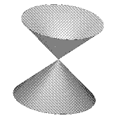
$A_{1}$	$A_{\infty}$	$D_{\infty}$

Figure 1: Morse type of non-isolated singularites

Remark 6.8

We conjecture the above formula to hold for all singularities with critical locus a curve $\Sigma$ and with transverse type $A_{1}$. However, the above proof does not apply, in particular not if the curve $\Sigma$ is not smoothable.

Theorem 6.9

The formula of theorem 6.7 is valid for all non-isolated hypersurface singularities in three space with one-dimensional critical locus of transverse type $A_{1}$:

$$2\sigma(f)=\chi(F_{+})-\chi(F_{-})$$

Proof.

Let $\Sigma\subset({\mathbb{C}}^{3},0)$ be the critical locus of $f$, described by a radical ideal $I$, so $f\in\int I$ and let $g\in I^{2}$ be generic. The statement holds for $g$, because for these a morsification does exist and thus we can apply the previous result. Also, there is an admissible deformation described by $F=tf+(1-t)g$ and where the curve $\Sigma$ is deformed trivially. By 6.6 we have $\sigma(g)=\sigma(f)+\sum\sigma_{i}(f_{i},p_{i})$, where the $(f_{i},p_{i}$ are the germs of singularties (of type $A_{1}$ of $D_{\infty}$ that split off in this deformation. As we know the truth for these singularities, we can conclude the truth of the statement for $f$ itself. ∎

Remark 6.10

(i) The formula 6.9 appears to holds for a much broader class of surface singularities with other transverse types, but it is not true without further assumptions. For example, the jacobian module $I/J_{f}$ for the sextic $f=(x^{2}+y^{2})^{3}-4x^{2}y^{2}z^{2}=0$ has $2t^{5}+3t^{6}+2t^{7}$ as Poincaré polynomial. So its dimension is seven, and thus the signature in any case is odd. In fact it can be computed to be equal to three. In contrast, the difference of the real Euler characterisics is eight.
(ii) From additivity of the Euler number one has

$$\chi(F_{+})+\chi(F_{-})+\chi(F_{0})=2$$

where $\chi(L_{0})$ is the Euler number of the real link $L_{0}:=S^{n-1}\cap F_{0}$ of the singularity. In turn, this number is equal to

$$\chi(L_{0})=\sum_{i}\sigma(\Sigma_{i})$$

where the sum runs over the real half-branches $\Sigma_{i}$ of the curve $\Sigma$, and where $\sigma(\Sigma_{i})$ denotes the $\sigma$ of the singularity transverse to $\Sigma_{i}$. Formulated differently,

$$\sum_{i}\sigma(\Sigma_{i})=N-D$$

where $N$ denotes the nunmber of naked half-branches (transverse type $\pm(x^{2}+y^{2})$) and $D$ the number of dressed half-branches (transverse type $x^{2}-y^{2}$).

6.3 A signature theorem for projective curves

A homogenous polynomial $f\in{\mathbb{R}}[x,y,z]$ defines a cone $X:=\{f=0\}\subset{\mathbb{R}}^{3}$ which is the same as a projective curve $C\subset{\mathbb{P}}^{2}({\mathbb{R}})$. Furthermore, if $f$ has even degree, $f$ has a well defined sign for each point in the complement of the curve. We put $V_{+}:=\{(x:y:z)\in{\mathbb{P}}^{2}({\mathbb{R}}):f(x,y,z)>0\}$ and $V_{-}:=\{(x:y:z)\in{\mathbb{P}}^{2}({\mathbb{R}}):f(x,y,z)<0\}$ The singularities of the cone $X$ is a finite union of lines, namely the cone over the singularities of $C$. The curve $C$ has ordinary double points, precisely if the the transverse type outside the origin ist $A_{1}$.

Theorem 6.11

Let $f\in{\mathbb{R}}[x,y,z]$ be a homogenous polynomial of even degree defining a curve with only double points as singularities. Then

$$\sigma_{f}=\chi(V_{+})-\chi(V_{-}).$$

Proof.

(see also [A]) Let $F_{+}$ and $F_{-}$ denote the positive and negativ Milnor fibre of $f$ in ${\mathbb{R}}^{3}$. The restriction of the canonical projection ${\mathbb{R}}^{3}\setminus\{0\}\rightarrow{\mathbb{P}}^{2}({\mathbb{R}})$ to the Milnor fibres $F_{+}\rightarrow V_{+}$ and $F_{-}\rightarrow V_{-}$ is an unramified $2:1$ covering. For the Euler characteristics we thus obtain $\chi(F_{+})=2\chi(V_{+})$, $\chi(F_{-})=2\chi(\mathcal{V}_{-})$. hence the result follows from 6.9. ∎

Example 6.12

The signature of the cone over the nodal quartic defined by

$$(x^{2}+y^{2})^{2}+3x^{2}y-y^{3}=0$$

is $\sigma=-3$, we see $\chi_{+}=0$ and $\chi_{-}=3$. The signature of the cone over the quartik with a $D_{4}$-singularity defined by

$$2(x^{2}+y^{2})^{2}+10y(3x^{2}-y^{2})+11(x^{2}+y^{2})-3=0$$

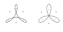
Figure 2: Two Quartics

is $\sigma=-4$, the Euler numbers are $\chi_{+}=0$ and $\chi_{-}=4$. Figure 2 shows the curves and the defined regions.

Example 6.13

Depending on the situation, the signature can be used to find real components of algebraic curves.

$$\begin{array}[]{ccc}\psfig{}&\psfig{}&\psfig{}\\ \sigma=2&\sigma=0&\sigma=-2\end{array}$$

Figure 3: Relative position of a line and a cubic with signature of product quartic

In figure 3, the signature of the quartic, consisting of the shown cubic and a moving test line, separates the different topological positions of the line relative to the cubic.

Example 6.14

In figure 4 the signature of the shown quartic separates the relative topological configuration of the two quadrics.

$$\begin{array}[]{ccccc}\psfig{}&\psfig{width=48.36958pt}&\psfig{}&\psfig{}&\psfig{}\\ \sigma=1&\sigma=0&\sigma=-1&\sigma=-2&\sigma=-3\end{array}$$

Figure 4: Relative position of two quadrics and signature of the product quartic

7 Some open problems

We have shown that the self-duality of the Koszul-complex leads in the almost complete intersection case to a self-duality of $I/J$. In the real case one can define a signature. For the special case of Jacobi-modules of hypersurface singularities with one-dimensional singular locus this signature was related, in special cases, to Euler-characteristics of positive and negative Milnor fibre, which can be seen as a generalisation of the theorem formulated in [A].

$\bullet$ What is the topological meaning of the signature in general? In other words, proper generalisation of the Eisenbud-Levine theorem? We have seen that for Jacobi-modules of a special class of hypersurfaces with one-dimensional singular locus there is a direct relation with the Euler characteristic of the positive and negative Milnor fibre. But we have also seen that this relation does not hold in all examples. The more special question is: for exactly what class of singularities with one-dimensional singular locus is theorem 6.7 is true?

$\bullet$ In the complete intersection case the pairing on $P/J$ factors over the multiplication map. For an almost complete intersection the non-degenerate pairing

$$I/J\times I/J\longrightarrow K$$

is also $P$-linear, but there is no evident ’multiplication map’ to factor over.

Conjecture 7.1

In the case where $I$ is a radical ideal one has:

1) The pairing on $I/J$ factors over the multiplication map

$$I/J\times I/J\longrightarrow I^{2}/IJ$$

2) If $I/J\neq 0$ then The $P$-module $I^{2}/IJ$ has a one-dimensional socle.

3) The socle of $I^{2}/IJ$ is generated by the Jacobian determinant

$$h:=\left|\begin{array}[]{ccc}\frac{\partial f_{1}}{\partial x_{1}}&\ldots&\frac{\partial f_{1}}{\partial x_{n}}\\ \ldots&\ldots&\ldots\\ \frac{\partial f_{n}}{\partial x_{1}}&\ldots&\frac{\partial f_{n}}{\partial x_{n}}\\ \end{array}\right|$$

We note that for radical ideals $I$ in three variables one always has $\dim(I/J)=\dim(I^{2}/IJ)$, by [dJvS1] For non-radical ideals $I$ the statements of the conjecture often hold, but again the function $f=(x^{2}+y^{2})^{3}-x^{2}y^{2}z^{2}$ provides a counterexample. Here $I^{2}/IJ$ has Poincaré polynomial $2t^{10}+2t^{11}$, however, the Hessian $h$ sits in degree $12$. The series $(x^{3}+y^{3})^{p}-x^{p}y^{p}z^{p}$ provides further examples.

The pairing on $I/J$ is symmetric, but we do not know a good algebraic proof of this fact. Of course it would be explained by the above conjecture.

$\bullet$ Is there a way to exhibit a self-dual resolution resolution of $I/J$ as $P$-module?
If

$$0\longrightarrow F_{n-1}\longrightarrow\ldots\longrightarrow F_{1}\longrightarrow P\longrightarrow P/I$$

is a free resolution over $P$, the map $P/J\longrightarrow P/I$ can be covered by a map of the Koszul-complex $\wedge^{\bullet}$ to $F_{\bullet}$ giving a diagram

$$\begin{array}[]{cccccccccc}\wedge^{n-1}&\longrightarrow&\wedge^{n-2}&\longrightarrow&\ldots&\wedge^{1}&\longrightarrow&P&\longrightarrow&P/J\\ \downarrow&&\downarrow&&&\downarrow&&\downarrow&&\downarrow\\ F_{n-1}&\longrightarrow&F_{n-2}&\ldots&\longrightarrow&F_{1}&\longrightarrow&P&\longrightarrow&P/I\\ \end{array}$$

Applying $Hom_{P}(-,P)$ to the diagram, and using $Hom(\wedge^{p},P)=\wedge^{n-p}$ we obtain also maps

$$\begin{array}[]{ccccccccc}F_{1}^{*}&\longrightarrow&F_{2}^{*}&\longrightarrow&\ldots&\longrightarrow&F_{n-2}^{*}&\longrightarrow&F_{n-1}^{*}\\ \downarrow&&\downarrow&&&&\downarrow&&\downarrow\\ \wedge^{n-1}&\longrightarrow&\wedge^{n-2}&\longrightarrow&\ldots&\longrightarrow&\wedge^{2}&\longrightarrow&\wedge^{1}\\ \end{array}$$

These two diagrams can be put on top of each other:

$$\begin{array}[]{ccccccccc}F_{1}^{*}&\longrightarrow&F_{2}^{*}&\longrightarrow&\ldots&\longrightarrow&F_{n-2}^{*}&\longrightarrow&F_{n-1}^{*}\\ \downarrow&&\downarrow&&&&\downarrow&&\downarrow\\ \wedge^{n-1}&\longrightarrow&\wedge^{n-2}&\longrightarrow&\ldots&\longrightarrow&\wedge^{2}&\longrightarrow&\wedge^{1}\\ \downarrow&&\downarrow&&&&\downarrow&&\downarrow\\ F_{n-1}&\longrightarrow&F_{n-2}&\longrightarrow&\ldots&\longrightarrow&F_{2}&\longrightarrow&F_{1}\\ \end{array}$$

If this were a double complex, the total complex would be a self-dual resolution of $I/J$ of the right length, see [P3]. Unfortunately, is is not clear that the maps always can be chosen as to obtain a double complex.

$\bullet$ Furthermore, one might ask for generalisations going further than almost complete intersections and look for self-dual pieces in the Koszul-homology. It is not clear how such a theorem might look like: there are simple examples of sequences $f_{1},\ldots,f_{n}$ in $P$ with $\dim(P/J)=2$, but for which $H^{0}_{\mathfrak{m}}(P/J)$ is not a Gorenstein module. The homogeneous function $f=(x+y)(xu)^{2}+(u+v)(xv)^{2}+(x+u+v)(yu)^{2}+(y+u)(yv)^{2}$ is singular along the union of two planes defined by the ideal $(x,y)\cap(u,v)$, so the locus defined by $J=J_{f}$ is two-dimensional. The module $H^{0}_{\mathfrak{m}}(P/J)$ is computed to have

$$6t^{4}+13t^{5}+15t^{6}+9t^{7}$$

as Poincaré series, so it is not Gorenstein.

Acknowledgement: The first author wants to thank D. Eisenbud for showing interest in the pairing in an early stage of this work and asked the question as to the meaning of the signature in the real case. The work was part of the Ph. D. thesis of the second author. The authors thank further R. Pellikaan exchange of ideas and T. de Jong for suggesting the argument used in 6.9.

References

- [AFN] K. Aoki, T. Fukuda and T. Nishimura, On the number of branches of the zero locus of a map germ , In: Topology and computer science (Atami, 1986), 347–-363, (Kinokuniya, Tokyo, 1987).
- [AGV] , V. I. Arnold, S. M. Guzein-Zade, A. N. Varchenko, Singularities of differentiable maps. Vol. I and II. Monographs in Mathematics 83. (Birkhäuser Boston, 1988).
- [A] V. I. Arnold,The index of a singular point of a vector field, the Petrovskiĭ-Oleĭnik inequalities, and mixed Hodge structures, Funct. Anal. Appl. 12 no.1 (1978), 1-–14.
- [BH] , W. Bruns, J. Herzog, Cohen-Macaulay rings, Cambridge studies in adv. math. 39, Cambridge University Press, 1993.
- [CE] H. Cartan and S. Eilenberg, Homological Algebra, (Princeton University Press, 1956).
- [D] N. Dutertre, On topological invariants associated with a polynomial with isolated critical points. Glasg. Math. J. 46 (2004), no. 2, 323–-334.
- [DSW] A. Dimca, M. Saito, L. Wotzlaw, A generalization of the Griffiths theorem on rational integrals. II. Michigan Math. J. 58 (2009), no. 3, 603-–625.
- [E] D. Eisenbud, Commutative Algebra with a View Toward Algebraic Geometry, (Springer, Berlin, 1995).
- [EG] W. Ebeling, S. M. Gusein-Zade, Indices of vector fields and 1-forms on singular varieties. Global aspects of complex geometry, 129-–169, (Springer, Berlin, 2006).
- [EL] D. Eisenbud and H. Levine, An algebraic formula for the degree of a map germ, Annals of Mathematics, 106 (1977), 19–44.
- [dJ] T. de Jong, The virtual number of points. I. Topology 29 (1990), no. 2, 175–184.
- [dJdJ] J. de Jong, T. de Jong, The virtual number of points. II. Topology 29 (1990), no. 2, 185–188.
- [dJvS1] T. de Jong and D. van Straten, A deformation theory for nonisolated singularities. Abh. Math. Sem. Univ. Hamburg 60 (1990), 177–208.
- [dJvS2] T. de Jong and D. van Straten, Disentanglements, In: Singularity theory and its applications, Part I (Coventry, 1988/1989), 199–211, Lecture Notes in Math., 1462, (Springer, Berlin, 1991).
- [GV] A. N. Varchenko, A. B. Givental, The period mapping and the intersection form. Funct. Anal. Appl. 16 (1982), no. 2, 7–-20.
- [K] G. M. Khimshiashvilli, On the local degree of a smooth map, Soobshch. Akad. Nauk. GruzSSR, 85(2) (1977), 309–311.
- [Ma] H. Matsumura, Commutative ring theory, (Cambridge Universtiy Press 1986).
- [Mi] J. Milnor, Singular points of complex hypersurfaces, Ann. Math. Stud. 61 (Princeton University Press, 1968).
- [MvS] J. Montaldi and D. van Straten, D. One-forms on singular curves and the topology of real curve singularities. Topology29 (1990), no.4, 501–510.
- [P1] R. Pellikaan, Finite determinacy of functions with nonisolated singularities. Proc. London Math. Soc. (3) 57 (1988), no. 2, 357–-382.
- [P2] R. Pellikaan, Deformations of hypersurfaces with a one-dimensional singular locus. J. Pure Appl. Algebra 67 (1990), no. 1, 49–71.
- [P3] R. Pellikaan, Projective resolutions of the quotient of two ideals. Nederl. Akad. Wetensch. Indag. Math. 50 (1988), no. 1, 65–84.
- [Sa] K. Saito, The higher residue pairings for a family of hypersurface singular points. Singularities, Part 2 (Arcata, Calif., 1981), 441-–463, Proc. Sympos. Pure Math. 40, (Amer. Math. Soc., Providence, RI, 1983).
- [Si] D. Siersma, Isolated line singularities. Singularities, Part 2 (Arcata, Calif., 1981), 485–496, Proc. Sympos. Pure Math. 40, (Amer. Math. Soc., Providence, RI, 1983).
- [vS] D. van Straten, On the Betti numbers of the Milnor fibre of a certain class of hypersurface singularities. In: Singularities, representation of algebras, and vector bundles (Lambrecht, 1985), 203–220, Lecture Notes in Math. 1273, (Springer, Berlin, 1987).
- [SS] G. Scheja und U.Storch, Über Spurfunktionen bei vollständigen Durchschnitten. J. Reine und Angew. Math. 278/279 (1975), 174–189.
- [Sz1] Z. Szafraniec, A formula for the Euler characteristic of a real algebraic manifold. Manuscripta Math. 85 (1994), no. 3-4, 345–360.
- [Sz2] Z. Szafraniec, Topological degree and quadratic forms. J. Pure Appl. Algebra 141 (1999), no. 3, 299–314.
- [Sz3] Z. Szafraniec, Topological invariants of real Milnor fibres. Manuscripta Math. 110 (2003) 2, 159–169.
- [V] A. N. Varchenko, Local residue and the intersection form in vanishing cohomology, Izv. Akad. Nauk SSSR Ser. Mat. 49 (1985), no. 1, 32–54.
- [Wa] T. Warmt, Gorenstein-Dualität und topologische Invarianten von Singularitäten, PhD thesis, Johannes-Gutenberg Universität Mainz (2003).
- [We] H. Weber, Lehrbuch der Algebra, Bd. 1, (Verlag Vieweg und Sohn, Braunschweig 1898).