Efficient Maximum Likelihood Estimation of a 2-D Complex Sinusoidal Based on Barycentric Interpolation

Abstract

This paper presents an efficient method to compute the maximum likelihood (ML) estimation of the parameters of a complex 2-D sinusoidal, with the complexity order of the FFT. The method is based on an accurate barycentric formula for interpolating band-limited signals, and on the fact that the ML cost function can be viewed as a signal of this type, if the time and frequency variables are switched. The method consists in first computing the DFT of the data samples, and then locating the maximum of the cost function by means of Newton’s algorithm. The fact is that the complexity of the latter step is small and independent of the data size, since it makes use of the barycentric formula for obtaining the values of the cost function and its derivatives. Thus, the total complexity order is that of the FFT. The method is validated in a numerical example.

Index Terms— Frequency estimation, parameter estimation, fast Fourier transform (FFT), barycentric interpolation, sampling.

1 Introduction

The estimation of the parameters of a complex sinusoidal in either one or two dimensions is a pervasive problem in signal processing. For this problem, the maximum likelihood (ML) principle provides an optimal estimator, in the sense that it achieves the Cramer-Rao bound at relatively low signal-to-noise ratios. Yet in practice this estimator is deemed too complex, due to the associated maximization problem. In rough terms, the situation is that, though the ML cost function can be regularly sampled using the FFT efficiently, the localization of its maximum requires some search procedure, and here is where the high computational burden seems unavoidable. This observation was first stated by B. G. Quinn in [1], where it was shown that a Gauss-Newton iteration may fail to find the global maximum of the cost function, if the initial iteration is taken from the DFT of the data samples (without zero padding). This has led several researches to give up the ML approach, and look for sub-optimal estimators with lower computational burden, [2, 3]. However, in some references [4, 5, 6] there has been an attempt to recover the initial ML approach, based on two arguments. The first is that it is feasible to approximately locate the maximum of the ML cost function, simply by looking for the DFT sample with largest module. Besides, the accuracy of this coarse localization can be improved by zero padding. And the second is that it is possible to interpolate the cost function close to this location from the nearby DFT samples with some accuracy, since it is a smooth function. These arguments, if properly exploited, make it possible to improve the performance significantly, with a complexity similar to that of the FFT. The purpose of this paper is to go one step further in this direction, and show that it is feasible to perform this interpolation with high accuracy from a small number of DFT samples, so that the actual ML estimate can be obtained with the complexity of a single FFT. The key lies in viewing the DFT as a band-limited signal in the frequency variable.

The basic concept in this paper is first presented in the next section in the context of time-domain interpolation. It is a simple an efficient technique to interpolate a band-limited signal from a small number of samples with high accuracy. Then, the estimation problem in one dimension is introduced in Sec. 3, where it is shown that the method in the next section is actually the key for an efficient solution, if the independent variable is properly interpreted. Afterward, Sec. 4 presents the extension of the method in Sec. 3 to the two-dimensional case, and finally Sec. 5 contains a numerical example.

2 High accuracy interpolation of a band-limited signal and its derivatives

Given a band-limited signal ${\mathrm{s}}(t)$ with two-sided bandwidth $B$, a usual task is to interpolate its value from a finite set of samples surrounding $t$. If the sampling period is $T$ with $BT<1$ (Nyquist condition), and $2P+1$ samples are taken symmetrically around $t$, then this task consists in finding a set of coefficients $a_{p}(u)$ such that the formula

$${\mathrm{s}}(t)\approx\sum_{p=-P}^{P}{\mathrm{s}}((n-p)T)a_{p}(u)$$ (1)

is accurate, where $t=nT+u$ is the modulo-$T$ decomposition of $t$,

$$n\equiv\lfloor t/T+1/2\rfloor,\;\;u\equiv t-nT.$$ (2)

For fixed $u$, the $a_{p}(u)$ can be obtained numerically using filter optimization techniques [7]. Yet this approach is cumbersome, if not only ${\mathrm{s}}(t)$ but also its derivatives must be interpolated for varying values of $u$ efficiently. Recently, a so-called barycentric interpolator was derived in [8] that solves this problem satisfactorily. This interpolator takes the form

$${\mathrm{s}}(nT+u)\approx\left.\sum_{p=-P}^{P}\frac{{\mathrm{s}}((n-p)T)w_{p}}{u-pT}\right/\sum_{p=-P}^{P}\frac{w_{p}}{u-pT},$$ (3)

where $w_{p}$ is a set of constants which are samples of a fixed function ${\mathrm{w}}(t)$, [$w_{p}\equiv{\mathrm{w}}(pT)$]. In [8], this function is given by the formula

$${\mathrm{w}}(t)\equiv\frac{{\mathrm{\Gamma}}(t/T+P+1){\mathrm{\Gamma}}(-t/T+P+1){\mathrm{g}}(t)}{{\mathrm{L}}^{\prime}(t)},$$ (4)

where ${\mathrm{\Gamma}}(\cdot)$ is the Gamma function, ${\mathrm{g}}(t)$ is the pulse

$$\frac{{\mathrm{sinc}}((1-BT)\sqrt{(t/T)^{2}-(P+1)^{2})}}{{\mathrm{sinc}}(j(1-BT)(P+1))},$$ (5)

and ${\mathrm{L}}(t)$ is the polynomial

$${\mathrm{L}}(t)\equiv\prod_{p=-P}^{P}(t-pT).$$ (6)

(See [8] for further details.) The fact is that the error of (1) decreases exponentially with trend ${\mathrm{e}}^{-\pi(1-BT)P}$. In practice this means that a small $P$ is enough to obtain high accuracy. Besides, as shown in [8], Eq. (1) can be differentiated with low complexity, so as to interpolate the differentials of ${\mathrm{s}}(t)$ of any order, and (3) can be evaluated using only one division. This interpolator will be the fundamental tool in the next section.

3 ML frequency estimation: 1-D case

Consider a signal ${\mathrm{z}}(t)$ consisting of an undamped exponential with complex amplitude $a$ and frequency $f_{o}$, contaminated by complex white noise ${\mathrm{n}}(t)$ of zero mean and variance $\sigma^{2}$,

$${\mathrm{z}}(t)={\mathrm{e}}^{j2\pi f_{o}t}+{\mathrm{n}}(t).$$ (7)

For simplicity, $f_{o}$ is assumed to lie in $[-1/2,1/2[$. Next, assume that $M$ samples of ${\mathrm{z}}(t)$ are taken at instants $m_{1},m_{1}+1,\ldots,m_{1}+M-1$ with $m_{1}\equiv-\lceil M/2\rceil$. The maximum likelihood estimation of $f_{o}$ from these samples is the argument that maximizes the cost function

$${\mathrm{L}}(f)\equiv|{\mathrm{c}}(f)|^{2},$$ (8)

where ${\mathrm{c}}(f)$ is the correlation

$${\mathrm{c}}(f)\equiv\sum_{m=m_{1}}^{m_{1}+M-1}{\mathrm{z}}(m){\mathrm{e}}^{-j2\pi fm}.$$ (9)

Since ${\mathrm{c}}(f)$ is the DFT of the samples ${\mathrm{z}}(m)$, the maximum of ${\mathrm{L}}(f)$ can be approximately located by selecting a frequency spacing $\Delta f$ such that $1/\Delta f$ is a power of two, and then computing the samples

$${\mathrm{c}}(k\Delta f)\equiv\sum_{m=m_{1}}^{m_{1}+M-1}{\mathrm{z}}(m){\mathrm{e}}^{-j2\pi km\Delta f},$$ (10)

by means of a radix-2 FFT algorithm. The cost of this operation is only ${\mathrm{O}}(M\log M)$. This way, it is possible to obtain a frequency $k_{o}\Delta f$ that lies close to the true abscissa of the maximum of ${\mathrm{L}}(f)$. However, if $\hat{f}_{o}$ is this abscissa, the approximation of $\hat{f}_{o}$ using $k_{o}\Delta f$ is very inaccurate. In this situation, the accuracy can be improved by reducing $\Delta f$ (over-sampling), but then the computational burden becomes high.

The barycentric interpolator in the previous section provides an efficient method to obtain $\hat{f}_{o}$ The key idea is that the correlation ${\mathrm{c}}(f)$ in (9) is a band-limited signal in the $f$ variable of bandwidth $2m_{1}$, i.e, the variable $f$ in (9) plays the same role as the variable $t$ in (1). Also, ${\mathrm{L}}(f)$ is band-limited with bandwidth $4m_{1}$. So, the method of sampling the correlation using the FFT, and then looking for its maximum module can be reformulated taking into account these information. First, since ${\mathrm{L}}(f)$ has two-sided bandwidth $4m_{1}$, it is necessary to sample this function with a spacing smaller than its Nyquist period $1/(4m_{1})$, in order to coarsely locate its maximum. This implies that a factor-two zero padding is enough to ensure the localization of the maximum of ${\mathrm{L}}(f)$. And second, since ${\mathrm{c}}(f)$ has bandwidth $2m_{1}$, it can be interpolated using the barycentric formula in (1) with $2m_{1}$ in place of $B$, and $\Delta f$ in place of $T$, i.e,

$${\mathrm{c}}(f)\approx\left.\sum_{p=-P}^{P}\frac{{\mathrm{c}}((k-p)\Delta f)w_{p}}{\gamma-p\Delta f}\right/\sum_{p=-P}^{P}\frac{w_{p}}{\gamma-p\Delta f},$$ (11)

where $f=k\Delta f+\gamma$ is the modulo-$\Delta f$ decomposition of $f$ defined as in (2). If $\tilde{{\mathrm{c}}}(f)$ denotes the approximation to ${\mathrm{c}}(f)$ in (11), then one may replace the problem of maximizing $\tilde{{\mathrm{L}}}(f)$ with that of maximizing

$$\tilde{{\mathrm{L}}}(f)\equiv|\tilde{{\mathrm{c}}}(f)|^{2}$$ (12)

Besides, the maximum of this function is close to the abscissa of the largest FFT sample in (10), $k_{o}\Delta f$.

Since $P$ is small and there is a coarse estimate of the maximum abscissa, the maximization of (12) is a low-complexity problem that can be solved using standard numerical methods. Given that the differentials of the barycentric interpolator can be easily computed [8, Sec. IV], a suitable numerical method is Newton’s algorithm, in which the $r$th iteration $f_{r}$ is refined using

$$f_{r+1}=f_{r}+\tilde{{\mathrm{L}}}^{\prime}(f_{r})/\tilde{{\mathrm{L}}}^{\prime\prime}(f_{r})$$ (13)

where

$$\begin{array}[]{r@{\,=\,}l}\displaystyle\tilde{{\mathrm{L}}}^{\prime}(f)&\displaystyle\frac{2}{M}\mathrm{Re}\{\tilde{{\mathrm{c}}}^{\prime}(f)\tilde{{\mathrm{c}}}(f)^{*}\},\\ \displaystyle\tilde{{\mathrm{L}}}^{\prime\prime}(f)&\displaystyle\frac{2}{M}(\mathrm{Re}\{\tilde{{\mathrm{c}}}^{\prime\prime}(f)\tilde{{\mathrm{c}}}(f)^{*}\}+|\tilde{{\mathrm{c}}}^{\prime}(f)|^{2}).\end{array}$$ (14)

This process can be initiated with $f_{1}=k_{o}\Delta f$, and a small number of iterations (3 to 5) is enough to obtain $\hat{f}_{o}$.

The computational burden of this method is given by that of the FFT, i.e, it is ${\mathrm{O}}(M\log M)$, and it yields the actual ML estimate of $f_{o}$.

4 ML frequency estimation: 2-D case

The method in the previous section can be extended to two-dimensional signals with non-essential changes. For this, it is only necessary to consider two variables, $t_{1}$ and $t_{2}$, and repeat the same interpolation procedure. The initial model, equivalent to (7), is

$${\mathrm{z}}(t_{1},t_{2})={\mathrm{e}}^{j2\pi(f_{1,o}t_{1}+f_{2,o}t_{2})}+{\mathrm{n}}(t_{1},t_{2}).$$ (15)

Next, this signal is sampled at the integer pairs $(m,n)$ for $m_{1}\leq m<m_{1}+M$ and $n_{1}\leq n<n_{1}+N$, with $m_{1}\equiv-\lceil M/2\rceil$, $n_{1}\equiv-\lceil N/2\rceil$. The 2-D equivalent of the cost function in (8) is

$${\mathrm{L}}(f_{1},f_{2})\equiv|{\mathrm{c}}(f_{1},f_{2})|^{2},$$ (16)

where ${\mathrm{c}}(f_{1},f_{2})$ is the correlation

$${\mathrm{c}}(f_{1},f_{2})\equiv\sum_{m=m_{1}}^{m_{1}+M-1}\sum_{n=n_{1}}^{n_{1}+N-1}{\mathrm{z}}(m,n){\mathrm{e}}^{-j2\pi(f_{1}m+f_{2}n)}.$$ (17)

This function can be sampled with spacings $\Delta f_{1}$, $\Delta f_{2}$ using a radix-2 2-D FFT. These samples provide a frequency pair $(k_{1,o}\Delta f_{1},$ $k_{2,o}\Delta f_{2})$ that lies close to the maximum of ${\mathrm{L}}(f_{1},f_{2})$. Then, it is possible to set up an interpolation formula like (11) but in two dimensions,

$$\begin{array}[]{l}\displaystyle{\mathrm{c}}(f_{1},f_{2})\approx\sum_{p_{1}=-P_{1}}^{P_{1}}\sum_{p_{2}=-P_{2}}^{P_{2}}\\ \displaystyle{}\hskip 14.22636pt\frac{{\mathrm{c}}((k_{1}-p_{1})\Delta f_{1},(k_{2}-p_{2})\Delta f_{2})w_{1,p_{1}}w_{2,p_{2}}}{(\gamma_{1}-p_{1}\Delta f_{1})(\gamma_{1}-p_{1}\Delta f_{1})}\cdot\\ \displaystyle{}\hskip 25.6073pt\Big{[}\sum_{p_{1}=-P_{1}}^{P_{1}}\frac{w_{1,p_{1}}}{\gamma_{1}-p_{1}\Delta f_{1}}\sum_{p_{2}=-P_{2}}^{P_{2}}\frac{w_{2,p_{2}}}{\gamma_{2}-p_{2}\Delta f_{2}}\Big{]}^{-1},\end{array}$$ (18)

where $f_{1}=k_{1}\Delta f_{1}+\gamma_{1}$ and $f_{2}=k_{2}\Delta f_{2}+\gamma_{2}$ are the modulo decompositions, and $w_{1,p_{1}}$ and $w_{2,p_{2}}$ are the barycentric weights corresponding to bandwidths $2m_{1}$ and $2n_{1}$, and truncation indices $P_{1}$ and $P_{2}$, respectively. If $\tilde{{\mathrm{c}}}(f_{1},f_{2})$ denotes the formula in (18), the problem of maximizing ${\mathrm{L}}(f_{1},f_{2})$ can be substituted by the problem of maximizing

$$\tilde{{\mathrm{L}}}(f_{1},f_{2})\equiv|\tilde{{\mathrm{c}}}(f_{1},f_{2})|^{2}.$$ (19)

Finally, the Newton iteration for this problem is

$$(f_{1,r+1},f_{2,r+1})=(f_{1,r},f_{2,r})+\mathcal{H}\tilde{{\mathrm{L}}}^{-1}\nabla\tilde{{\mathrm{L}}},$$ (20)

where $\nabla\tilde{{\mathrm{L}}}$ and $\mathcal{H}\tilde{{\mathrm{L}}}$ are the gradient and Hessian of $\tilde{{\mathrm{L}}}$ respectively, evaluated at $(f_{1,r},f_{2,r})$. These functionals are

$$\nabla\tilde{{\mathrm{L}}}=\frac{2}{MN}\,\mathrm{Re}\{\nabla\tilde{{\mathrm{c}}}\tilde{{\mathrm{c}}}^{*}\}$$ (21)

and

$$\mathcal{H}\tilde{{\mathrm{L}}}=\frac{2}{MN}\,\mathrm{Re}\{\mathcal{H}\tilde{{\mathrm{c}}}\,\tilde{{\mathrm{c}}}^{*}+\nabla\tilde{{\mathrm{c}}}\nabla\tilde{{\mathrm{c}}}^{\mathrm{H}}\},$$ (22)

where $\nabla{\tilde{{\mathrm{c}}}}$ and $\mathcal{H}\tilde{{\mathrm{c}}}$ are the corresponding gradient and Hessian of $\tilde{{\mathrm{c}}}$.

Since the evaluation of $\tilde{{\mathrm{c}}}(f_{1},f_{2})$ has a small cost which is independent of either $M$ or $N$, the complexity is given by the 2-D FFT, i.e, it is ${\mathrm{O}}(MN\log(MN))$. Note that sub-optimal methods like that in [3] have complexity ${\mathrm{O}}(MN(M+N))$, that is, the method in this section yields the ML estimate and, besides, has a smaller complexity order.

5 Numerical examples

Let ${\mathrm{\phi}}(f,t)$ denote the value delivered by the barycentric formula in (3), when the input signal is the undamped exponential ${\mathrm{s}}(t)={\mathrm{e}}^{j2\pi ft}$. Since the functions to interpolate in this paper are sums of exponentials like ${\mathrm{e}}^{j2\pi ft}$, a simple way to assess the interpolation accuracy is to evaluate the maximum module of ${\mathrm{e}}^{j2\pi fu}-{\mathrm{\phi}}(f,u)$, for $|u|\leq T/2$ and $f$ varying in $[-B/2,B/2]$, i.e, to assess the spectrum function

$${\mathrm{E}}(f)\equiv\max_{|u|\leq T/2}|{\mathrm{e}}^{j2\pi fu}-{\mathrm{\phi}}(f,u)|.$$ (23)

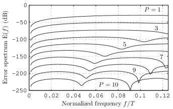
Fig. 1: Error spectrum ${\mathrm{E}}(f)$ of the barycentric interpolator in (3) for several truncation indices $P$.

Fig 1 shows ${\mathrm{E}}(f)$ for $BT=0.25$ and several truncation indices $P$. Note that any accuracy can be achieved uniformly in $[-B/2,B/2]$, by slightly increasing $P$.

In order to test the interpolation error in a specific example, a 2-D undamped exponential with $M=500$, $N=651$ and frequencies $f_{o,1}=0.234452$ and $f_{o,2}=-0.143254$ was generated. Then, complex white noise was added, so that the signal-to-noise ratio was $S/N=5$ dB. Fig. 2 shows the interpolation error for the cost function ${\mathrm{L}}(f_{1},f_{2})$, defined by

$$\epsilon\equiv\frac{\max_{f_{1},f_{2}}|{\mathrm{L}}(f_{1},f_{2})-\tilde{{\mathrm{L}}}(f_{1},f_{2})|}{\max_{f_{1},f_{2}}{\mathrm{L}}(f_{1},f_{2})},$$ (24)

for varying truncation index $P$. Again, it is clear that any accuracy can be achieved by slightly increasing $P$.

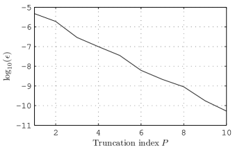
Fig. 2: Truncation index $P$ versus the $\log_{10}$ of the maximum interpolation error ($\log_{10}\epsilon$) for the cost function ${\mathrm{L}}(f_{1},f_{2})$.

Next, two estimators were compared in this example. To describe them, let $\mathbf{Z}$ denote the data matrix obtained by sampling (15) as described in that section,

$$[\mbox{\boldmath$\mathbf{Z}$\unboldmath}]_{m,n}\equiv{\mathrm{z}}((m_{1}+m-1)T_{1},(n_{1}+n-1)T_{2}),$$ (25)

and let $\mbox{\boldmath$\mathbf{u}$\unboldmath}_{1}$, $\mbox{\boldmath$\mathbf{v}$\unboldmath}_{1}$ denote its first left and right singular vectors, respectively. The first method consisted in computing the 1-D ML estimator from $\mbox{\boldmath$\mathbf{u}$\unboldmath}_{1}$ and $\mbox{\boldmath$\mathbf{v}$\unboldmath}_{1}$ so as to obtain the respective estimations of $f_{o,1}$ and $f_{o,2}$,

$$\begin{array}[]{l}\displaystyle\hat{f}_{o,1}=\arg\max_{f}\Big{|}\sum_{m=1}^{M}[\mbox{\boldmath$\mathbf{u}$\unboldmath}_{1}]_{m}{\mathrm{e}}^{-j2\pi(m_{1}-1+m)f}\Big{|}^{2}.\\ \displaystyle\hat{f}_{o,2}=\arg\max_{f}\Big{|}\sum_{n=1}^{N}[\mbox{\boldmath$\mathbf{v}$\unboldmath}_{1}]_{n}{\mathrm{e}}^{-j2\pi(n_{1}-1+n)f}\Big{|}^{2}.\end{array}$$ (26)

The actual estimations $\hat{f}_{o,1}$ and $\hat{f}_{o,2}$ were computed from $\mbox{\boldmath$\mathbf{u}$\unboldmath}_{1}$ and $\mbox{\boldmath$\mathbf{v}$\unboldmath}_{1}$ by applying the 1-D method in Sec. 3 to each of them. This method had complexity ${\mathrm{O}}(MN(M+N))$, since it involved the computation of the singular vectors $\mbox{\boldmath$\mathbf{u}$\unboldmath}_{1}$ and $\mbox{\boldmath$\mathbf{v}$\unboldmath}_{1}$, and is equivalent to the method in [3]. The second method computed the actual ML estimator from $\mathbf{Z}$ using the method in Sec. 4, and its complexity was just ${\mathrm{O}}(MN\log(MN))$. For the values of $M$ and $N$ given above, the over-sampling factors were $2.048$ and $1.523$, respectively, i.e, the FFT had size 1024 in both dimensions.

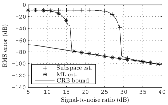
Fig. 3: Root-Mean-Square (RMS) error of the subspace and ML estimators, together with the Cramer-Rao bound.

Fig. 3 shows the root-mean-square (RMS) error for the first estimator, termed subspace estimator, for the second estimator (interpolated ML estimator), and the Cramer-Rao bound. The threshold performance of the second is clearly superior.

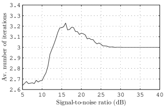
Fig. 4: Average number of iterations required by the Newton method.

Finally, Fig. 4 shows the average number of iterations that required the interpolated ML estimator, which was roughly equal to three.

6 Conclusions

A method has been presented that allows one to compute the maximum likelihood (ML) estimation of a complex 2-D sinusoidal, with the complexity of the fast Fourier transform (FFT). First, it is recalled in the paper that a band-limited signal can be interpolated with high accuracy from a small number of samples, if the sampling frequency is somewhat higher than the Nyquist frequency. Besides, a specific barycentric formula is proposed to perform this kind of interpolation. And second, it is shown that the ML cost function for the estimation of a complex 2-D (and 1-D) sinusoidal can be viewed as a band-limited signal, if the time and frequency variables are switched. Finally, these two results are combined in a method that is able to deliver the ML estimate with the complexity order of the FFT, which is based on Newton’s algorithm.

References

- [1] B. G. Quinn, “A fast efficient technique for the estimation of frequency,” Biometrika, vol. 78, no. 3, pp. 489–497, 1991.
- [2] B. G. Quinn, “Estimating frequency by interpolation using Fourier coefficients,” IEEE Transactions on Signal Processing, vol. 42, no. 5, pp. 1264–1268, 1994.
- [3] H. C. So, F. K. W. Chan, W. H. Lau, and C. Chan, “An efficient approach for two-dimensional parameter estimation of a single-tone,” IEEE Transactions on Signal Processing, vol. 58, no. 4, pp. 1999–2009, Apr 2010.
- [4] E. Aboutanios and B. Mulgrew, “Iterative frequency estimation by interpolation on Fourier coefficients,” IEEE Transactions on Signal Processing, vol. 53, no. 4, pp. 1237–1242, Apr 2005.
- [5] M. D. Macleod, “Fast nearly ML estimation of the parameters of real or complex single tones or resolved multiple tones,” IEEE Transactions on Signal Processing, vol. 46, no. 1, pp. 141–148, Jan 1998.
- [6] I. Perisa and J. Lindner, “Employing simple FFT-interpolation for improved complex tone detection and fine estimation,” in 3rd International Symposium on Wireless Communication Systems, 2006. (ISWCS ’06), 6-8 2006, pp. 744 –748.
- [7] T. I. Laakso, V. Välimäki, M. Karjalainen, and U. K. Laine, “Splitting the Unit Delay,” IEEE Signal Processing Magazine, vol. 13, no. 1, pp. 30–60, Jan 1996.
- [8] J. Selva, “Design of barycentric interpolators for uniform and nonuniform sampling grids,” IEEE Transactions on Signal Processing,, vol. 58, no. 3, pp. 1618 –1627, Mar 2010.