Abstract

Given an atlas of the brain and a number of injections to be performed in order to map out the connections between parts of the brain, we propose an algorithm to compute the coordinates of the injections. The algorithm is designed to sample the brain in the most homogeneous way compatible with the separation of brain regions. It can be applied to other species for which a neuroanatomical atlas is available. The computation is tested on the annotation at a resolution of 25 microns corresponding to the Allen Reference Atlas, which is hierarchical and consists of 209 regions. The resulting injections are being used for the injection protocol of the Mouse Brain Architecture project. Due to its large size and layered structure, the cerebral cortex is treated in a separate algorithm, which is more adapted to its geometry.

Introduction

Neuroanatomy is experiencing a renaissance thanks to the huge amount of data generated through molecular biology and image-processing [1, 2]. Brain regions can be separated in a data-driven way and compared to brain regions defined by classical neuroanatomy [3, 4]. Ongoing data generation at the Mouse Brain Architecture project aims to construct the full matrix of directed connections between parts of the brain [5]. In order to do so, various tracers are injected in vivo into the brain of a mouse. Cryosectioning of the brain after a survival period produces a series of images showing the projections of the injection sites.

The present note presents the algorithm used to compute the coordinates of the injections. The problem we address is a coding problem in the sense that a three-dimensional object, with complex internal structure, has to be represented by a set of points, and the number of points in the set is much smaller than the number of voxels in the numerical atlas encoding the internal structure. The algorithm is not specific to the atlas or number of injections we considered. The injection coordinates can be recomputed if a different number of injections is chosen, or if a different atlas is used. This allows the protocol to be extended to other species for which a neuroanatomical atlas is available. For species that do not have a cerebral cortex for instance, the special treatment of the cortex that is made in one of the loops of the algorithms will simply not be executed. The corresponding Matlab code is available upon request, to be executed using an atlas formatted into a three-dimensional grid by the user.

Given an atlas of the brain, we have to compute the coordinates of $I$ injections in the left hemisphere in such a way that these injection sites encode the atlas. The computation of coordinates has to satisfy the following two constraints:
1. Sampling constraint. In order to explore the brain efficiently, injections must not be too far from each other.
2. Separation constraint. In order to assign the origin of the tracers to a definite brain region, injections must not be too close to the boundaries of the regions.

If the brain had no internal structure, the atlas would consist of a single big region. Both constraints would be satisfied by filling the brain with a hexagonal sphere packing, with some exclusion zone around the surface of the brain. Injections would be placed at the centers of the spheres. They would form a crystal structure. The algorithm we propose applies this method to regions within the brain. The whole set of injections is therefore not quite regular: it resembles a crystal with defects induced by the boundaries of brain regions. Across a large brain region, the injections sites will look like a crystal. In a cluster of very small brain regions, they will look like an amorphous pile of points, with the coordinates of the points dictated mostly by the geometry of the boundaries of the regions (see Figures (9) and (8) for illustrations).

The structure of the paper is as follows. The algorithm used to choose regions and to compute coordinates is first described in pseudocode. Relevant orders of magnitudes for the sizes of brain regions in the Allen Reference Atlas are then derived. This leads to an estimate of a reasonable security distance to be used to satisfy the separation constraint. The computational techniques used to estimate distances from boundaries are then exposed. They are based on solutions to the eikonal equation. The cerebral cortex is treated in a separate way due to its large size and layered structure. Results are presented for the mouse brain. We used the Allen Reference Atlas[6], which consists of 209 regions, with a resolution of 25 microns, intersected with the left hemisphere of the brain. The value $I=250$ was dictated by time constraints on the production of data for the Mouse Brain Architecture project. The algorithm can be used to encode other atlases, with another number $I$ of injection sites. Geometric properties of the resulting injection coordinates (pairwise distances and distances to boundaries of brain regions) are then studied in order to check that the sampling and separation constraints are resonably satisfied.

Algorithm

Given an atlas $\mathcal{A}$ of the left hemisphere of the brain (i.e. a hierarchical partition of the left hemisphere of the brain, endowed with a natural tree structure), and given the total number of injections $I$ to be placed, the algorithm reads as the following pseudocode:

1. Choose the targeted brain regions.
1.1 Compute the critical size for a targeted region: $V_{inj}=V_{tot}/I$, where $V_{tot}$ is the total volume of the left hemisphere of the brain.
1.2 For each region in the atlas $\mathcal{A}$ that is a leaf of the tree, compute its volume. If it is larger than $V_{inj}$, declare the region to be one of the targeted regions, and cut the corresponding leaf.
Otherwise lump the region with is parent region on the tree, and cut the corresponding leaf.
1.3 Repeat the procedure until the root of the tree is reached.

2. Define a security distance $\sigma$: distances between injections and boundaries of neuroanatomical regions should be larger than $\sigma$ in order to satisfy the separation constraint. The value of $\sigma$ is estimated below for the left hemisphere of the mouse brain.

3. For each targeted region $r$:
3.1 Compute the number $I_{r}$ of injections to be placed in the region, under the constraint $\sum_{r}I_{r}=I$.
3.2 If $I_{r}=1$, place the injection at the centroid of the region.
Otherwise, intersect the region with a sphere packing, and adjust the radius of the spheres so that exactly $I_{r}$ centers of spheres are in the region, and at distances from the boundary that exceed $\sigma$. If this fails, retry with a reduced value of sigma.

Given the large size of the cerebral cortex and its layered structure, it deserves a separate study in the mouse brain. Injections into the cortex are performed as a series of pulses along the trajectory of the needle. Given the sampling and separation constraints, these trajectories must be distributed as line segments intersecting an average layer of the cerebral cortex at sites that are homogeneously distributed on the layer. This gives rise to a intrinsically two-dimensional algorithm, described in a separate subsection, to be executed in the case of cerebral cortex only. It should be skipped when the algorithm is applied to species for which the delineation of the cerebral cortex is problematic or impossible.

Choice of targeted regions

We used a numerical version of the Allen Reference Atlas on a grid of size $528\times 320\times 456$, with voxel side 25 micrometers. The volume of a voxel is therefore roughly 0.016 nanoliter. At this resolution, 209 regions of the left hemisphere can be detected. For each of them, we computed the percentage of the volume of the left hemisphere it occupies.

As $I$ injection sites have to be chosen in the atlas ($I=250$ for the Mouse Brain Architecture project), a region is declared to be too small to be targeted if its volume is smaller than the typical injection volume defined as $V_{inj}=V_{tot}/I$, where $V_{tot}$ is the volume of the brain (or of the left hemisphere of the brain if the atlas is restricted to the left hemisphere).

Security distances from boundaries of regions

In order to separate the regions, the injection sites should not be too close to the boundary of any of the regions. In order to ensure this in a systematic way, we need to define a security distance, denoted by $\sigma$. We would like to forbid the placement of any injection site within $\sigma$ of the boundary of any region (however, this can fail for a fixed value of $\sigma$ in the case of regions that are very thin in one direction; the algorithm handles such cases by decreasing sigma until the sites have some room to be included). We present a simple scaling argument to derive an estimate of $\sigma$ that serves as an initial value of the security distance in the algorithm. But first we have to define the way distances to surfaces are computed.

Let us denote by $\mathcal{V}$ the space occupied by the region of interest, say caudoputamen, in the left hemisphere. Its boundary is a surface, denoted by $\mathcal{B}$. As we need to know how far the injection sites are from the boundary, we need to compute the distance $h$ between every point of $\mathcal{V}$ and the boundary. This is achieved by solving the eikonal equation in $\mathcal{V}$, with boundary conditions on $\mathcal{B}$:

$$|\nabla h|=1\;\;{\mathrm{in}}\;{\mathcal{V}},$$ (1)

$$h=0\;{\mathrm{on}}\;{\mathcal{B}}.$$

The eikonal equation is solved using level-set methods, such as the ones described in [7]. If we think of the surface as an object emitting light, the value of the solution $h$ at a given point is the shortest optical path followed by light coming from the object, provided the light propagates in a medium with index 1 (the index of the medium is actually the r.h.s. of the eikonal equation, as this equation is the Euler–Lagrange equation associated to an action equal to the optical path [8]). Another intuitive interpretation of the eikonal equation (1) is in terms of combustion: if the boudary $\mathcal{B}$ is set on fire, and the fire propagates in a homogeneous medium, $h(x)$ is the time at which point $x$ in the medium will be touched by the fire. This interpretation gives rise to the level-set algorithm in a natural way.

Having solved the eikonal equation, we can assess how well the separation constraint is satisfied. Injections should be comfortably far from the boundary of the region. So we define a security region given by points inside $\mathcal{V}$ whose distance from the boundary is larger than a security value, denoted by $\sigma$, which can be estimated based on the packing density of a regular hexagonal sphere packing. As the packing density for a hexagonal packing is

$$d=\frac{\pi}{3\sqrt{2}},$$

a first guess for the security value corresponds to a situation where spheres of radius $\sigma$ are hexagonally packed in the volume $V_{tot}$, without any dislocation

$$I\times\frac{4\pi}{3}\sigma^{3}=d\times V_{tot},$$

i.e.

$$\sigma=\left(\frac{V_{tot}}{4\sqrt{2}I}\right)^{1/3}\simeq 500\;{\mathrm{microns}}$$

for the left hemisphere of the mouse brain with $I=250$, which can be difficult to achieve for very thin regions. Hence this value will be the initial value of the security distance in the algorithm, and will be lowered until the desired number of injections can be hexagonally packed in the region, with all the distances to boundary larger than the security value. In particular, for the region labelled ’Striatum’, which consists of several small subregions of striatum lumped together (larger subregions such as nucleus accumbens and caudoputamen, are targeted regions and receive several injections of their own), the security distance has to be reduced.

For each targeted region, given the solution $h$ of the eikonal equation with boundary condition at the boundary of the region (meaning internal boundary on a grid), the set of voxels within the region for which $h$ is larger than $\sigma$ will be referret to as the security region. As some of the hemisphere will not be used for injections because it does not fall into any security region, the minimal values of distances to boundaries obtained at the end of the algorithm will be smaller on average than the initial value of $\sigma$. See the discussion section for statistics on the distances to boundaries.

Computation of injection sites in a given brain region

In every brain region (apart from the cerebral cortex that will be treated separately, the injections are placed at the centers of speres in a hexagonal packing of regular spheres, whose radius is calibrated so that there are the desired number of injection sites in the region. There is some freedom in translations, dilations and rotations of the packing, which has not been used so far to maximize the average distance to the boundary, as the first configuration found was accepted.

If there is just one injection to be made in the region, its coordinates are taken to be those of the centroid $C_{r}$ of the security region ${\mathcal{S}}_{r}$, which is the point within the security region that minimizes the variance:

$$C_{r}={\mathrm{argmin}}_{C}\sum_{x\in{\mathcal{S}}_{r}}(x-C)^{2}.$$

In case the security region ${\mathcal{S}}_{r}$ is convex, the coordinates of $C_{r}$ are just the averages of the coordinates of the points in ${\mathcal{S}}_{r}$, as the average is the quantity that minimizes the variance.

If more injections are to be placed in the region, a precomputed grid of injections is superposed onto the security regions (the axes of the packing coincide with those of the grid containing the atlas). The intersection between the grid and the security region contains a number of points that depends on just one parameter, which is the radius of the sphere packing. The algorithm tries a range of values of this parameter until the intersection contains exactly the desired number of injections. It can be that the number of points in the intersection jumps by large quantities, thereby missing the desired number of injections. This occurs for very singular, anisotropic regions. In such cases, the security distance $\sigma$ is lowered until a suitable value for the radius of the sphere packing exists.

Results for the mouse brain, using the Allen Reference Atlas and $I=250$ injections

We used a numerical version of the Allen Reference Atlas on a grid of size $528\times 320\times 456$, with voxel side 25 micrometers. The volume of a voxel is therefore roughly 0.016 nanoliter. At this resolution, 209 regions of the left hemisphere can be detected. For each of them, we computed the percentage of the volume of the left hemisphere it occupies. The results are contained in the tables at the end of the present note.

As $I=250$ injection sites have to be chosen in the atlas, a region is declared to be too small if its volume is smaller than the typical injection volume defined as $V_{inj}=V_{tot}/I$, where $V_{tot}\simeq 0.19\;{\mathrm{mL}}$ is the volume of the left hemisphere of the mouse brain. The value of $V_{inj}$ is roughly $0.7$ microliters, corresponding to 0.4 percent of the volume of the left hemisphere.

As described in step 1.2 of the algorithm, one starts with the leaves of the hierarchical annotation with 209 indices. If the volume of a leaf is smaller than the critical volume $V_{inj}$, it is lumped with its parent, otherwise the leaf is declared to be one of the targeted regions. The leaves are then ’cut’ and this procedure is repeated until the root of the tree is reached. Some regions in the Allen Reference ATlas [6], such as ’Basic Cell Groups and Regions’, ’Cerebrum’ and ’Brain Stem’, do not form a clear anatomical pattern. We discarded them, and as their volumes add up to eight times the volume $V_{inj}$ taken by a single injection, eight injections were added to the number of injections into the cerebral cortex.

The first table of brain regions, Figure (1), shows a list of the leaves big enough to be targeted. The first column contains the name of the brain region, the second column, called ’Nb inj.’ contains the number of injections to be placed in the region, which is the closest integer to the quotient of the volume of the region by the critical volume $V_{inj}$. The third column, called ’Index’, contains the index of the region, which can be used to access the region in the full table of regions in the annotation. The fourth column, called ’Parent’, is the index in the main table of the parent of the region. The last column, called ’LumpedIndices’, gives the list of indices of regions (drawn from the full table), that have been lumped with the region because they are smaller than $V_{inj}$. As we are at the level of leaves in the annotation, the values contained in the third and fifth columns are the same.

Name	Nb Inj.	Index	Parent	LumpedIndices
Main olfactory bulb	10	6	5	6
Anterior olfactory nucleus	2	8	5	8
Piriform area	7	10	5	10
Ammon’s Horn	8	17	16	17
Dentate gyrus	3	18	16	18
Subiculum	2	20	19	20
Caudoputamen	13	24	23	24
Nucleus accumbens	3	26	25	26
Olfactory tubercle	2	28	25	28
Lateral septal nucleus	1	30	29	30
Pallidum- dorsal region	1	37	36	37
Substantia innominata	2	40	38	40
Ventral posterior complex of the thalamus	1	82	80	82
Zona incerta	1	110	107	110
Inferior colliculus	3	113	112	113
Superior colliculus- sensory related	1	118	112	118
Superior colliculus- motor related	3	120	119	120
Cerebellar cortex	26	209	204	209

Figure 1: Results of the first loop of the algorithmic choice of targeted regions. Leaves of the ’standard’ annotation (at ’level 7’ in the tree) whose volumes are larger than $V_{inj}$, with the numbers of injections they receive.

The result of the next step of the algorithm is presented in another table, Figure (2), organized in the same way. For instance one can see that the lateral group of the dorsal thalamus (index 57), was lumped with the lateral posterior nucleus of the thalamus (index 58) and the suprageniculate nucleus (index 59). The volumes of those three regions add up to $\simeq 0.48$ percentage points of the left hemisphere, which is just above the the fraction represented by $V_{inj}$, thus leading to one injection for this group of structures. Indeed the second column shows one injection. A coronal section intersecting the three regions is shown on figure (3). As the annotation is hierarchical, the resulting targeted region is connected.

Name	Nb Inj.	Index	Parent	LumpedIndices
Olfactory areas	4	5	4	5 7 9 11 12 13 14
Retrohippocampal region	7	19	15	19
Striatum-like amygdalar nuclei	2	32	22	32 33 34 35
Anterior group of the dorsal thalamus	1	49	48	49 50 51 52 53 54 55
Lateral group of the dorsal thalamus	1	57	48	57 58 59
Ventral group of the dorsal thalamus	1	80	75	80 81
Periaqueductal gray	2	124	119	124 125
Pons- sensory related	2	149	148	149 150 151 152 153
Pons- motor related	2	154	148	154 155 156 157 158 159 160 161 162
Vestibular nuclei	1	195	184	195 196 197

Figure 2: Results of the second loop of the algorithmic choice of targeted regions. Leaves of the ’standard’ annotation (at ’level 6’ in the tree) whose volumes are larger than $V_{inj}$ after being lumped with the leaves at level 7 that are too small to be targeted, with the numbers of injections they receive.

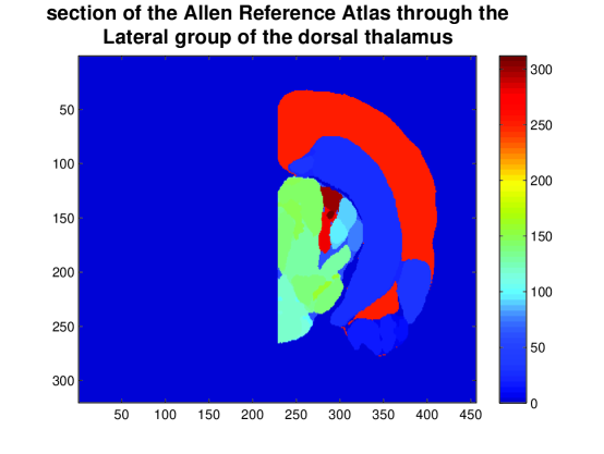
Figure 3: A coronal section of the standard annotation with non-empty intersection with the lateral group of the dorsal thalamus (value 259 in the color bar), the lateral posterior nucleus of the thalamus (value 279 in the color bar), and the suprageniculate nucleus (value 309 in the color bar). These three brain regions, when lumped together, make up a region just big enough to be targeted by one injection.

Brain Region	Volumetric fraction	Nb injections
Cerebral cortex	0.31	66
Retrohippocampal region	0.04	10
Hippocampal reg.	0.04	10
Olfactory areas	0.10	25
Medulla	0.06	15
Cerebellum	0.12	30
Thalamus	0.05	13
Pons	0.05	13
Striatum	0.09	23
Hypothalamus	0.04	10
Midbrain	0.08	20
Pallidum	0.02	5

Figure 4: The twelve big regions in the left hemisphere (coarsest non-hierarchical partition), with fractions of the volume occupied by each region, and numbers of injections received.

Full details of the whole hierachical procedure are not included in the present note, however the hierarchical atlas is compatible with the (non-hierarchical) partition of the left hemisphere into 12 regions, also provided by the Allen Reference Atlas [6]. The number of injections into each of those twelve regions, as shown in a separate table, Figure (4), is rougly proportional to the fraction of the volume of the left hemisphere it occupies.

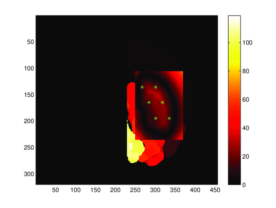
Figure 5: A coronal section of the caudoputamen, showing distances to the boundary and injection sites. A coronal section of the eikonal distances to the surface of the caudoputamen (computed in a small region enclosing the caudoputamen), overlaid onto the atlas, with six injections displayed as green stars. Distances in the colorbar are expressed in multiples of the voxel side, which is 25 microns. The characteristic level-set structure of the solution to the eikonal equation is manifest. The boundary of the caudoputamen in this section is at level 0.

Since the targeted regions are all treated separately by the algorithm, the injection grid looks locally like a crystal, but irregularities are induced by the boundaries between targeted brain regions. The locally hexagonal structure of the packing is visible in a coronal section of caudoputamen containing six of the thirteen injection sites computed in this structure. The eikonal distance function to the boundary of caudoputamen was only computed in a box containing caudoputamen, for the sake of speed. As the algorithm uses only values of the eikonal function inside the brain region.

The special case of the cerebral cortex

Figure 6 is a coronal section of the eikonal distance function to the boundary of the cerebral cortex in the mouse brain. By applying a mask onto the interior of the region, one can extract the surface inside the cerebral cortex that maximizes the distance to the boundary on any coronal section. This surface serves as an average layer, or average surface of the cerebral cortex.

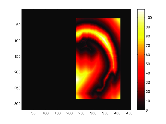
Figure 6: A coronal section of the eikonal distances to the surface of the cerebral cortex. Distances in the colorbar are expressed in multiples of the voxel side, which is 25 microns.

We would like to sample this surface in a homogeneous way. As it is not too singular, a reasonable tiling of the surface is induced by projecting a regular 2D hexagonal lattice (pictured in blue on the figure 7) onto the surface. The resulting sites are shown in magenta.

Given such a site, five injections are regularly distributed along a line oriented by the maximum gradient of the eikonal ditance across this site, so that the needle cut the brain along the shortest possible length. There are some boundary effects as the left-hemisphere has a vertical boundary on the right side that is not physical and can be caught by the algorithm.

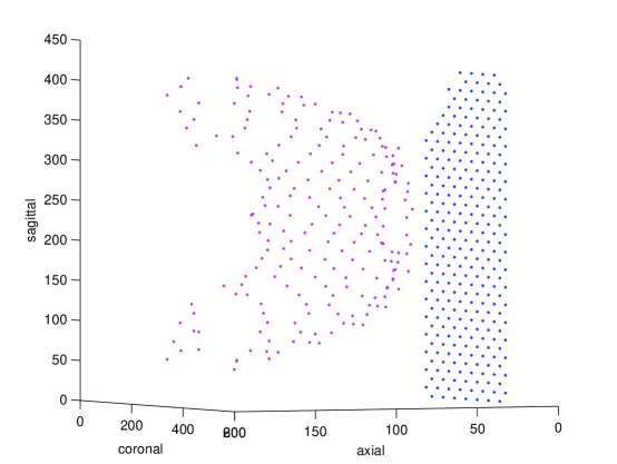
Figure 7: The intersections of the needle trajectory and the average surface of the cerebral cortex, in magenta. They are obtained by projecting the two-dimensional grid shown in blue onto the average surface.

The results of the algorithm in the left hemisphere of the mouse brain, with special treatment of the cerebral cortex, can be observed on a coronal section (Figure (8)) containing cortical injections, placed as columns of five pulses intersecting the average surface of the cortex, at sites sampling the average surface of the cortex. This coronal section also contains two injections targeting nucleus accumbens. From this figure it is clear that the local grids of injections going into each regions are slightly displaced in the rostrocaudal direction wrt the grid of injections into nucleus accumbens. Otherwise, all the other targeted regions, apart from cerebral cortex and nucleus accumbens, would have injection sites in this coronal plane. The boundary of nucleus accumbens therefore introduces an irregularity into the grid of injections.

A 3D plot of the injection targets, shown on Figure (9), looks locally like a crystal with many irregularities induces by boundaries of brain regions. On top of this crystal, the cortical injections look like a bunch of ordered spines.

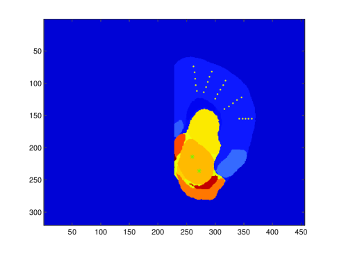
Figure 8: A coronal section with five ’columns of injections’ in the cerebral cortex (shown in yellow) and two injections into nucleus accumbens (shown in green).

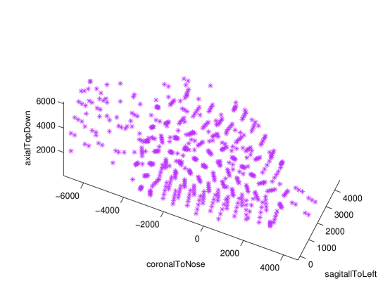
Figure 9: The injection targets shown as a cloud of magenta stars.

Discussion

Sampling constraint: pairwise distances within a region

If more than one injection is made in a region, the minimum pairwise distance between those injections should not be too different from $\sigma$, the spacing between vertices of a hexagonal packing that would fill the whole brain. Discrepancies between these minimal distances and $\sigma$ come from the shape of the region, for example in cases were the region is much more elongated in one dimension than in the other two. The average value of those distances is 762 microns, and the standard deviation is 433 microns.

Separation constraints: distances to the boundaries

As the security distance from the boundary has sometimes to be lowered in order to fit a hexagonal packing with the desired number of vertices, and as the centroid of a region can happen to be close to the boundary when the region is not convex, it is interesting to compute the minimal distances between the injections made in a region, and the boundary of this region (one just has to look up the values at injection sites of the eikonal distance functions that were evaluated when the security regions were determined). The mean distance to the boundary is 278 microns, close to $\sigma/2$, and the standard deviation is 72 microns. The exclusion of structures at the root of the tree, and the very procedure of excluding security regions from the computation, were expected to make the mean distance smaller than $\sigma$, with the same order of magnitude.

Distances between injections belonging to different regions

For a given pair of regions indexed by $r$ and $s$ in the set of targeted regions, one can compute the three following quantities:

- the distance $d_{rs}$ between the averages of the voxels in the regions $r$ and $s$,

- the minimal distance $m_{rs}$ between an injection site in $r$, and an injection site in $s$,

- the maximal distances $M_{rs}$ between an injection site in $r$, and an injection site in $s$.

The plots of sorted values $m$ and $M$ should reproduce roughly the behaviour of $d$. This is indeed what we infer for the tubular shape of the three plots shown on the neighboring figure.

Degrees of freedom and brain variability

The placement of single injections at the centroid of the brain regions (step 3.2 of the algorithm) would generalize naturally to larger sets of $k$ injections by minimizing the sums of squared distances to the injections across the region. This is the $k$-means algorithm [10]. Using this algorithm, or any other clustering algorithm applied to the set of coordinates of points within each brain region, would only change the step 3.2 of the algorithm. We did not choose to use $k$-means as the initialization step of the algorithm would introduce some more randomness. Of course the coordinates that are returned by our code are not the single admissible solutions to the algorithm. Each of the set of injections that consists of more than one injection has three translation invariances within the region, one for each coordinate axis. The amount of translation invariance is equal to the distance by which the injections can be collectively moved without any of them touching the boundary of the security region. Rotation degrees of freedom could also be considered, but this would break the alignment between planes containing several injections, and coronal sections of the atlas.

For practical purposes in the Mouse Brain Architecture project [5], the precision of the computations has to be matched by the surgical precision of the injections. As the positions of boundaries between regions are computed at a resolution of 25 microns, and as security distances from those boundaries are typically a few hundreds of microns, the geometric targets of the injections have to be reached with a comparable precision. The alignment between the coordinate systems in the Allen Atlas and in the live mouse is a first (geometric) step to take in order to achieve such a precision. A second (more biological) step consists in an estimation of the animal-to animal variability from a laser scan of the top of the skull. Both steps are taken algorithmically in a computer-guided stereotactic protocol presented in [9].

We treated the cerebral cortex seperately, and its characteristic layered structure will be sampled by columns of injections rather than by pointwise injections. The cerebellar cortex also has a layered structure, with layers separated by boundaries that could be described in a useful way in terms of level sets of an eikonal function. However, the boundary of the cerebellum has a folded profile that could not be resolved on the grid we used. The many more singularities of the boundary that are introduced by the layers would also make the result of the algorithm less robust against brain variability. The injection coordinates into cerebellar cortex were therefore computed using the three-dimensional algorithm based on sphere packings. Addressing the folded structure of the cerebellum in a computational way remains an open problem.

References

- 1. L. Ng, A. Bernard, C. Lau, C.C. Overly, H.-W. Dong, C. Kuan, S. Pathak, S.M. Sunkin, C. Dang, J.W. Bohland, H. Bokil, P.P. Mitra, L. Puelles, J. Hohmann, D.J. Anderson, E.S. Lein, A.R. Jones and M. Hawrylycz, An anatomic gene expression atlas of the adult mouse brain, Nature Neuroscience 12, 356 - 362 (2009).
- 2. L. Ng, M. Hawrylycz and D. Haynor, Automated high-throughput registration for localizing 3D mouse brain gene expression using ITK, Insight-Journal (2005).
- 3. J.W. Bohland, H. Bokil, S.D. Pathak, C.-K. Lee, L. Ng, C. Lau, C. Kuan, M. Hawrylycz and P.P. Mitra,Clustering of spatial gene expression patterns in the mouse brain and comparison with classical neuroanatomy, Methods (2010).
- 4. P. Grange and P.P. Mitra, Marker genes and the anatomy of the mouse brain, SFN Abstracts (2010), and in preparation.
- 5. J.W. Bohland et al., A proposal for a coordinated effort for the determination of brainwide neuroanatomical connectivity in model organisms at a mesoscopic scale, PLoS Computational Biology, 5(3), e1000334. PMID: 19325892.
- 6. H.-W. Dong, The Allen reference atlas: a digital brain atlas of the C57BL/6J male mouse, Wiley, 2007.
- 7. J.A. Sethian, Level Set Methods and Fast Marching Methods: Evolving Interfaces in Computational Geometry, Fluid Mechanics, Computer Vision and Materials Science, Cambridge University Press, 1999.
- 8. L.D. Landau and E.M. Lifshitz, Course of Theoretical Physics: Classical Mechanics, Vol. 1, Pergamon Press (1976, 3rd ed.).
- 9. P. Grange, T. Pologruto, V. Pinskiy, H. Wang, A. Khabbaz, S, Spring, L. Yu, J. Germann, M. Henkelman and P.P. Mitra, Computer-guided stereotactic injections for the Mouse Brain Architecture project, SFN Abstracts (2010, and in preparation.
- 10. J MacQueen, Some methods for classification and analysis of multivariate observations, Proceedings of the fifth Berkeley symposium (1967).
- 11. T. Hastie, R. Tibshirani and J. Friedman, The elements of statistical learning: data mining, inference, and prediction, Springer Series in Statistics (2009).