Possible observation sequences of Brans-Dicke wormholes

Abstract

The purpose of this study is to investigate observational features of Brans-Dicke wormholes in a case if they exist in our Universe. The energy flux from accretion onto a Brans-Dicke wormhole and the so-called “maximum impact parameter” are studied (the last one might allow to observe light sources through a wormhole throat). The computed values were compared with the corresponding ones for GR-wormholes and Schwarzschild black holes. We shown that Brans-Dicke wormholes are quasi-Schwarzschild objects and should differ from GR wormholes by about one order of magnitude in the accretion energy flux.

I Introduction

Different types of wormholes were extensively studied recently, especially in the framework of extended gravitational models. A lot of attention was paid to wormholes with massless scalar fields ellis ; bronn2 , in multidimentional theories clement1 ; clement2 ; clement3 ; bhawal ; dotti , in brane-world models anch ; bronn3 ; cam ; lobo1 , in semiclassical gravitation garat , and for different equations of state addressing the Dark Matter (or energy) issues sushkov . An important question naturally arises: would it be possible to distinguish between wormholes in different gravitational models using observational data available in the near future with better precision? There are several methods of compact objects’ study nowadays. Novikov and Shatsky shat1 ; shat2 ; shat3 have extracted distinctive features of gravitational lensing of light passing through the wormhole throat. It this work we focus on the possible observations of accretion disks around Brans-Dicke wormholes. According to the latest results, there are gas accretion disks or gas clouds around almost all galactic nuclei at distances from $0.1$ to $10^{3}$ pc urry . It is possible to evaluate the mass of the object through the gas flux in the clouds. The accretion speed allows to establish the existence of a surface and hence to determine the object’s nature because black holes and wormholes do not have any surface in the opposite to neutron stars that have the one. In the articles by T. Harko, Z. Kovacs and F.S.N. Lobo lobo2 ; lobo3 it was shown that fluxes of accretion onto different types of wormholes in General Relativity (GR) should differ by orders of magnitude. This approach therefore sounds meaningful. Our work is devoted to analogous considerations for Brans-Dicke wormholes and studies some of their topological aspects as well. We consider a stationary model of accretion disk lobo3 . Isotropic coordinates are used, as in the original Brans-Dicke formalism. All the results are written down in Planck units $c=G=\hbar=1$.

II Brans-Dicke wormholes

Brans-Dicke theory is a scalar-tensor gravitational model that leads to GR when the coupling constant $|\omega|\to\infty$. The action is:

$$S=\frac{1}{16\pi}\int d^{4}x\ \sqrt{-g}\ (\phi R+\frac{\omega}{\phi}\ g^{\mu\nu}\phi_{,\mu}\phi_{,\nu}+L_{matter}),$$ (1)

where $R$ is the Ricci scalar, $\phi$ is a scalar field, $g_{\mu\nu}$ is the metric tensor and $L_{matter}$ is the contribution of matter fields. The corresponding field equations are

$$\begin{split}R_{\mu\nu}-\frac{1}{2}\ g_{\mu\nu}R&=\frac{8\pi}{\phi}\ T_{\mu\nu}+\frac{\omega}{\phi^{2}}\left(\phi_{,\mu}\phi_{,\nu}-\frac{1}{2}\ g_{\mu\nu}\phi^{,\sigma}\phi_{,\sigma}\right)\\ &+\ \frac{1}{\phi}(\nabla_{\mu}\nabla_{\nu}\phi-g_{\mu\nu}\ \Box\phi),\\ \Box\phi&=\frac{8\pi T}{2\omega+3},\end{split}$$ (2)

where $T=T^{\mu}_{\mu}$, $T_{\mu\nu}$ is the stress-energy tensor and $\Box$ is d’Alembert operator.

There is a set of energy conditions in GR hock1 that imposes limits on the stress-energy tensor $T_{\mu\nu}$ caroll . To form a wormhole, one needs a matter that breaks the null energy condition but still remains stable. As usual, Jordan-Brans-Dicke theory allows gravity to influence matter via the space-time metric tensor. But the matter itself can change the metric both directly and via the additional scalar field. Thus, the gravitational constant $G$ depends on the scalar field which is variable in space and time. In the theory just the scalar field of Brans-Dicke plays the role of matter. This model does not restrict other kinds of matter or dust to be added of course, it just can not be completely matterless. As the Einstein tensor breaks the null energy condition due to its definition, the right part of expression (2) also breaks that condition.

There are four static spherically-symmetric solutions in Brans-Dicke theory brans but only the first and the fourth ones are independent. Scalar fields in Brans-Dicke model should satisfy the equation bhadra

$$\phi=\phi_{0}\left(1+\frac{1}{\omega+2}\ \frac{M}{r}\right)$$ (3)

up to first order in $1/r$. $M$ is the asymptotic mass of the wormhole at infinity. The forth solution breaks this condition so we consider only the first Brans-Dicke class of solutions with the metric

$$\begin{split}ds^{2}&=-\left(\cfrac{1-1/x}{1+1/x}\right)^{2l}dt^{2}+\left(1+\cfrac{1}{x}\right)^{4}\left(\frac{1-1/x}{1+1/x}\right)^{n}\\ &\quad\times\ (d\rho^{2}+\rho^{2}d\Omega^{2}),\\ \phi&=\phi_{0}\left(\cfrac{1-1/x}{1+1/x}\right)^{p}.\end{split}$$ (4)

Here $x=\rho/B$, $\quad l=1/\lambda$, $\quad n=(\lambda-C-1)/\lambda$, $\quad p=C/\lambda$, $\rho$ is the isotropic radial coordinate, $\lambda,\ B,\ C$ and $\omega$ are the constants related by brans :

$$\lambda=\sqrt{\cfrac{2\omega+3}{2\omega+4}},\quad B=\cfrac{M}{2\phi_{0}}\ \sqrt{\cfrac{2\omega+4}{2\omega+3}},\quad C=-\ \frac{1}{\omega+2}.$$ (5)

At infinity, the metric asymptotically approaches the Schwarzschild solution

$$ds^{2}=\left(\cfrac{1-\cfrac{r_{g}}{4\rho}}{1+\cfrac{r_{g}}{4\rho}}\right)^{2}dt^{2}-\left(1-\cfrac{r_{g}}{4\rho}\right)^{4}\left(d{\rho}^{2}+{\rho}^{2}d\Omega^{2}\right)$$

if $\omega\to\pm\ \infty$. The case $\omega\to+\ \infty$ corresponds to black holes and the one $\omega\to-\ \infty$ leads to wormholes. Thus $\lambda\to 1$, $C\to 0$ and $B\to M/2$ at the infinity.

Numerical values for the expressions in Brans-Dicke theory depend on the value of the coupling constant $\omega$. So it should be possible to fix $\left|\omega\right|$ from observational data. As it was shown by Agnese and La Camera, the discussed wormhole is traversable if $\omega<-\ 2$ agness . Thus the scalar field itself plays the role of the required exotic matter. Using Cassini experiments on PPN measuring, it is easy to find that $\left|\omega\right|>50000$ and only such values are considered.

III Flux and topology. Results

By solving geodesic equations, it is straightforward to establish that energy, angular momentum and angular velocity for particles on Keplerian orbits in the equatorial region of the accretion disk are:

$$\begin{split}\tilde{E}&=\left(\cfrac{x-\lambda}{x+\lambda}\right)^{l}\sqrt{\cfrac{x^{2}+\lambda^{2}-2x\ (C+1)}{x^{2}+\lambda^{2}-2x\ (C+2)}},\\ \tilde{L}&=\sqrt{\cfrac{2}{x}}\ B\ \cfrac{x^{2}-\lambda^{2}}{\sqrt{x^{2}+\lambda^{2}-2x\ (C+2)}}\left(\cfrac{x+\lambda}{x-\lambda}\right)^{l+p},\\ \Omega&=\cfrac{x}{B}\ \cfrac{1}{x^{2}-\lambda^{2}}\ \sqrt{\cfrac{2x}{x^{2}+\lambda^{2}-2x\ (C+1)}}\left(\cfrac{x-\lambda}{x+\lambda}\right)^{p+2l}.\end{split}$$ (6)

The flux of energy emitted from the disk surface during the accretion to the Brans-Dicke wormhole can be calculated numerically after substituting (6) into the expression pagethorn :

$$F(r)=-\ \frac{\dot{M_{0}}}{4\pi\sqrt{-g}}\ \frac{\Omega_{,r}}{(\tilde{E}-\Omega\tilde{L})^{2}}\int\limits_{r_{ms}}^{r}(\tilde{E}-\Omega\tilde{L})\ \tilde{L}_{,r}\ dr,$$ (7)

where $r_{ms}$ is the marginally stable orbit, and $\dot{M_{0}}$ is the accretion speed $\cfrac{dM}{dt}$. On Fig. 1–4 we compare the obtained values of angular velocity and moment, energy and energy flux of the accretion disk particles with the corresponding magnitudes for wormholes in GR and Schwarzschild black holes.

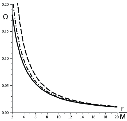
Figure 1: Angular velocities of the accretion disk particles ($\times 10^{-4}\ \mbox{rad}/\mbox{c}$) for wormholes in GR (dashdot line), Schwarzschild black hole (dash line) and Brans-Dicke wormhole (solid line) as a function of the normalized radius.

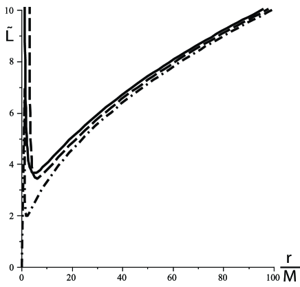
Figure 2: Angular moments of the accretion disk particles ($\times 10^{4}\ \mbox{cm}^{2}/\mbox{c}$) for wormholes in GR (dashdot line), Schwarzschild black hole (dash line) and Brans-Dicke wormhole (solid line) as a function the normalized radius.

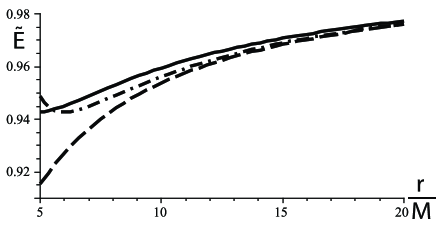
Figure 3: Energy of the accretion disk particles ($\mbox{cm}^{2}/\mbox{c}^{2}$) in mass unites for wormholes in GR (dashdot line), Schwarzschild black hole (dash line) and Brans-Dicke wormhole (solid line) as a function of the normalized radius.

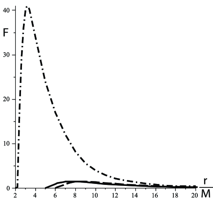
Figure 4: Energy flux of the accretion disk particles ($\times 10^{23}\ \mbox{erg}/\mbox{cm}^{2}/\mbox{c}$)for wormholes in GR (dashdot line), Schwarzschild black hole (dash line) and Brans-Dicke wormhole (solid line) as a function of the normalized radius.

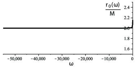
Figure 5: Wormhole’s throat radius in mass units as a function of the Brans-Dicke parameter $\omega$.

The wormhole throat is the surface with the minimal possible area surrounding the entry into another universe. The isotropic radial coordinate $\rho$ on the throat surface is given by

$$\rho_{0}=\cfrac{\sqrt{2}B}{2}\left(\cfrac{2\ |\omega+1|\pm\sqrt{-8-6\omega}}{\sqrt{(2\omega+3)(\omega+2)}}\right).$$ (8)

If $\left|\omega\right|>50000$ the throat radius in arbitrary coordinates is $r_{0}=2M$ (Fig. 5) with a high precision. Hence, it coincides with the Schwarzschild gravitational radius of the black hole with corresponding mass.

The maximum impact parameter $h_{max}$ that allows to observe light sources from the other universe shat1 for Brans-Dicke wormholes in almost the full range of $\omega$ is $h_{max}=3\sqrt{3}M\approx 5.18M$ (Fig. 6). This expected result confirms the fact that the observable Brans-Dicke wormholes must be quasi-Schwarzschild (for them $\omega\to-\ \infty$ by definition).

The marginally stable orbit in the considered model was found numerically and has a value $r_{ms}\approx 5M$.

One can find the stress-energy tensor for the Brans-Dicke scalar field from:

$$\begin{split}T_{\mu\nu}&=\frac{\omega}{\varphi^{2}}\left(\varphi_{,\mu}\varphi_{,\nu}-\frac{1}{2}\ g_{\mu\nu}\varphi^{,\sigma}\varphi_{,\sigma}\right)\\ &+\frac{1}{\varphi}\ (\nabla_{\mu}\nabla_{\nu}\varphi-g_{\mu\nu}\ \Box\varphi).\end{split}$$ (9)

Therefore

$$\begin{split}T_{rr}&=\cfrac{\omega}{2}\ C^{2}l^{2}\left(\cfrac{2}{\rho x\left(1-1/x^{2}\right)}\right)^{2}\left(\cfrac{1-1/x}{1+1/x}\right)^{2Cl}\\ &+\ \cfrac{1}{\rho^{2}}\left(\cfrac{1-1/x}{1+1/x}\right)^{Cl}\left\{1-\left(1+\cfrac{1}{x}\right)^{4}\right.\\ &\times\left.\left(\cfrac{1-1/x}{1+1/x}\right)^{2\left(1-Cl-l\right)}\right\}\\ &\times\left[\left(-\cfrac{2Cl}{x\left(1-1/x^{2}\right)}-1\right)^{2}-\cfrac{4Cl}{x\left(1-1/x^{2}\right)^{2}}-1\right].\end{split}$$ (10)

The study of this expression can reveal new properties of the scalar field and will be the subject or further researches.

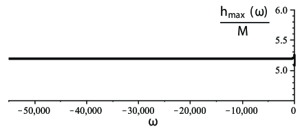
Figure 6: Wormhole’s maximum impact parameter in mass units as a function of the Brans-Dicke parameter $\omega$.

IV Conclusions

We have calculated the flux from accretion onto the Brans-Dicke wormhole. It is important to underline that the observer at infinity sees only the integral flux. The distribution of the flux of energy emitted form the accretion disk is almost Gauss one, so its integral flux is proportional to the maximum of the energy one. These maxima are just the values to be compared. The maximum energy for the accretion onto spherically-symmetric wormholes in GR is one order of magnitude larger that the one for the accretion onto the Brans-Dicke wormhole or on a Schwarzschild black hole. As shown here, for the last two types the values or the energy maximum are almost the same. As allowed values for $\omega$ are already restricted, measuring of the energy flux allows to test the considered model and can help to distinguish between different types of compact objects in future.

The throat radius and maximum impact parameter for a Brans-Dicke wormhole were found. We show that these values do not differ from the ones associated with a quasi-Schwarzschild wormhole. According to the Birkhoff theorem the Schwarzschild metric is the most common spherically-symmetric one in a curved space-time. This solution by itself describes the black hole and does not lead to such objects as wormholes, but the studied wormholes tend to the Schwarzschild metric at the infinity. So it is possible to claim that Brans-Dicke wormholes are asymptotically Schwarzschild. This fact allows to search for them basing on future observational data with more accuracy.

V Acknowledgements

Authors would like to thank Prof. Aurelien Barrau and Dr. Alexander Shatsky for the useful discussions on the subject of this work. The work was supported by the Federal Agency on Science and Innovations of Russian Federation via State Contract No. 02.740.11.0575.

References

- (1) H.G. Ellis, J. Math. Phys. 14, 104 (1973)
- (2) K.A. Bronnikov, Acta Phys. Polon. B 4, 251 (1973)
- (3) G. Clement, Gen. Rel. Grav. 16, 131 (1984)
- (4) G. Clement, Gen. Rel. Grav. 16, 477 (1984)
- (5) G. Clement, Gen. Rel. Grav. 16, 491 (1984)
- (6) B. Bhawal, S. Kar, Phys. Rev. D 46, 2464 (1992)
- (7) G. Dotti, J. Oliva, R. Troncoso, Phys. Rev. D 75, 024002 (2007)
- (8) L.A. Anchordoqui, S.E. PerezBergliaffa, Phys. Rev. D 62, 067502 (2000)
- (9) K.A. Bronnikov, S.-W. Kim, Phys. Rev. D 67, 064027 (2003)
- (10) M. La Camera, Phys.Lett. B 573, 27 (2003)
- (11) F.S.N. Lobo, Phys. Rev. D 75, 064027 (2007)
- (12) R. Garattini, F.S.N. Lobo, Class. Quant. Grav. 24, 2401 (2007)
- (13) S. Sushkov, Phys. Rev. D 71, 043520 (2005)
- (14) A.A. Shatsky, Phys.Usp. 52, 811 (2009)
- (15) A.A. Shatsky, I.D. Novikov, N.S. Kardashev, Phys.Usp. 51, 457 (2008)
- (16) I.D. Novikov, N.S. Kardashev, A.A. Shatsky, Phys.Usp. 50, 965 (2007)
- (17) C.M. Urry, P. Padovani, Publ. Astron. Soc. of the Pacific 107, 803 (1995)
- (18) T. Harko, Z. Kovacs, F.S.N. Lobo, Phys. Rev. D 78, 084005 (2008)
- (19) T. Harko, Z. Kovacs, F.S.N. Lobo, Phys. Rev. D 79, 064001 (2009)
- (20) S.W. Hawking and G.F.R. Ellis, The Large Scale Structure of Space-Time, (Cambridge, Cambridge University Press: 1973)
- (21) S.M. Carroll, M. Hoffman, M. Trodden, Phys. Rev. D 68, 023509 (2003)
- (22) C.H. Brans, R.H. Dicke, Phys. Rev. 124, 925 (1961)
- (23) A. Bhadra, K. Sarkar, Mod. Phys. Lett. A 20, 1831 (2005)
- (24) A.G. Agnese, M. La Camera, Phys. Rev. D 51, 2011 (1995)
- (25) D.N. Page, K.S. Thorn, Astrophys. J. 191, 499 (1974)