Measuring Spin Accumulations with Current Noise

Abstract

We investigate the time-dependent fluctuations of the electric current injected from a reservoir with a non-equilibrium spin accumulation into a mesoscopic conductor. We show how the current noise power directly reflects the magnitude of the spin accumulation in two easily noticeable ways. First, as the temperature is lowered, the small-bias noise saturates at a value determined by the spin accumulation. Second, in the presence of spin-orbit interactions in the conductor, the current noise exhibits a sample-dependent mesoscopic asymmetry under reversal of the electric current direction. These features provide for a purely electric protocol for measuring spin accumulations.

Noise measurements on non-equilibrium electric currents are very efficient probes of the dynamics and nature of the charge carriers bla00 . At low temperature, the classical Johnson-Nyquist noise is suppressed and quantum effects govern the behavior of the surviving shot noise. In the mesoscopic regime, the noise power $S$ is reduced below its uncorrelated Poisson value $S_{0}=2|q|\langle I\rangle$, where $\langle I\rangle$ is the average electric current, by the Fano factor $F=S/S_{0}$. The value of $F$ depends on the electronic dynamics. For instance, one finds $F=1/3$ in diffusive systems and $F=1/4$ in ballistic chaotic systems bla00 ; bee03 . Alternatively, shot noise measurements have determined the charge $|q|$ of current-carrying quasiparticles in normal-metal/superconductor junctions and in the fractional quantum Hall effect bla00 ; bee03 ; rez98 . In this manuscript we further illustrate the usefulness of current noise measurements by showing how they can reveal the magnitude of non-equilibrium spin accumulations. Our results provide for a purely electric protocol to measure spin accumulations, which has the potential to quantitatively determine their magnitude. It therefore goes one step further than the optical methods used so far to detect magneto-electrically generated spin accumulations she1 ; she2 . Alternatively, the noise measurement we propose, coupled with an electric measurement of the spin Hall and inverse spin Hall effects she3 ; she4 ; she5 , can provide key experimental information on the conversion between spin accumulations and spin currents.

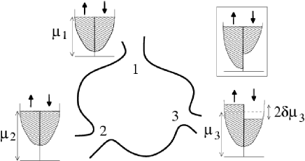
Figure 1: Three-terminal quantum dot connected to two unpolarized electron reservoirs (labeled 1 and 2) and one reservoir (3) with a non-equilibrium spin accumulation. Top right inset: a ferromagnetic reservoir with an equilibrium spin accumulation (a case we do not consider in this paper).

A number of works have investigated charge current noise from polarized reservoirs. Reference erl05 suggested using current and noise measurements in the single-channel limit to measure the spin injection efficiency from a ferromagnet for weak spin flip scattering. Other related works have pointed out that noise measurements in hybrid paramagnetic/ferromagnetic structures can reveal information on the relative orientation of the ferromagnets tser and on the spin relaxation processes in the paramagnet Mish ; lam ; belzig ; Nag . These results have been at least partially confirmed by numerical simulations nik . In non-interacting systems, current cross-correlations have a sign determined by the statistics of the charge carriers. Investigations of a single-level interacting fermionic quantum dot coupled to ferromagnetic leads have demonstrated the emergence of positive (boson like) current cross-correlations for certain relative orientations of the polarizations bruder . In all these instances, only ferromagnetic, i.e.,  equilibrium polarizations were considered. Below we show that non-equilibrium spin accumulations generate fundamentally different electric current noises. Our main findings are that (i) at low enough temperature, the small-bias noise saturates at a value reflecting the spin accumulation, and (ii) in the presence of spin-orbit interactions, the current noise exhibits a sample-dependent, mesoscopic asymmetry under reversal of the electric current direction. These two features appear only in the presence of non-equilibrium spin accumulations.

We consider a system such as the one sketched in Fig. 1, where a mesoscopic conductor is connected via multichannel leads to $M$ external reservoirs, $\alpha=1,2,\ldots,M$, at electro-chemical potentials $\mu_{\alpha}=(\mu_{\alpha\uparrow}+\mu_{\alpha\downarrow})/2$ and with non-equilibrium spin accumulations $\delta\mu_{\alpha}=(\mu_{\alpha\uparrow}-\mu_{\alpha\downarrow})/2$, along reservoir-dependent axes de- fined by unit vectors ${\bf m}_{\alpha}=(m_{\alpha x},m_{\alpha y},m_{\alpha z})$. We use the linear response scattering approach to transport to write the zero-frequency noise power in units of $(e^{2}/h)$ as bla00 ; nik

$${S}_{\alpha\beta} = \sum_{\gamma\delta}\sum_{(m,\sigma)\in\gamma}\sum_{(n,\sigma^{\prime})\in\delta}\int dE\;A_{\gamma\delta}^{m,\sigma;n,\sigma^{\prime}}\left(\alpha;E\right)A_{\delta\gamma}^{n,\sigma^{\prime};m,\sigma}\left(\beta;E\right)\;\left[f_{\gamma}^{\sigma}\left(1-f_{\delta}^{\sigma^{\prime}}\right)+f_{\delta}^{\sigma^{\prime}}\left(1-f_{\gamma}^{\sigma}\right)\right]\,,$$ (1)

where $f_{\gamma}^{\sigma}$ is the Fermi function for electrons with spin $\sigma=\pm$ along ${\bf m}_{\gamma}$ in terminal $\gamma$, and the sums run over all terminals $\gamma$ and $\delta$ (including $\alpha$ and $\beta$), all channels $m\in\gamma$ and $n\in\delta$, and all spin orientations $\sigma,\sigma^{\prime}=\pm$. We defined

$$A_{\gamma\delta}^{m,\sigma;n,\sigma^{\prime}}\left(\alpha;E\right) =\delta_{mn}\delta_{\sigma\sigma^{\prime}}\delta_{\alpha\gamma}\delta_{\alpha\delta}-[s_{\alpha\gamma}^{\dagger}(E)s_{\alpha\delta}(E)]_{m,\sigma;n,\sigma^{\prime}}\,,$$ (2)

where $s_{\alpha\gamma}$ denotes the $2N_{\alpha}\times 2N_{\gamma}$ subblock of the scattering matrix of the total system, corresponding to scattering from lead $\gamma$ to lead $\alpha$, $N_{\alpha,\gamma}$ being the number of channels in those leads. This assumes that $N_{\alpha}$ is spin-independent in all leads, and we will comment on the case $N_{\alpha\uparrow}\neq N_{\alpha\downarrow}$ later. Equation (1) differs from Eq. (52) in Ref. bla00 in that spin indices are explicitly written down here. All our calculations below are current-conserving, gauge invariant, and satisfy linear response reciprocity relations, as they should. We assume that the temperature, applied voltages, and spin accumulations are low enough that the scattering matrix is essentially constant in the energy interval where the square bracket in Eq. (1) does not vanish. We then substitute $A_{\gamma\delta}^{m,\sigma;n,\sigma^{\prime}}\left(\alpha;E\right)\rightarrow A_{\gamma\delta}^{m,\sigma;n,\sigma^{\prime}}\left(\alpha;E_{\rm F}\right)$, define

$${\cal F}^{\sigma\sigma^{\prime}}_{\gamma\delta}\equiv\int dE\left[f_{\gamma}^{\sigma}\left(1-f_{\delta}^{\sigma^{\prime}}\right)+f_{\delta}^{\sigma^{\prime}}\left(1-f_{\gamma}^{\sigma}\right)\right]\;,$$ (3)

and introduce the two-terminal symmetry coefficients

$${\cal F}^{SS}_{\gamma\delta} = \frac{1}{4}\sum_{\sigma\sigma^{\prime}}{\cal F}^{\sigma\sigma^{\prime}}_{\gamma\delta}\;,\;\;{\cal F}^{AA}_{\gamma\delta}=\frac{1}{4}\sum_{\sigma\sigma^{\prime}}\sigma\sigma^{\prime}{\cal F}^{\sigma\sigma^{\prime}}_{\gamma\delta}\;,\qquad$$ (4a)

$${\cal F}^{AS}_{\gamma\delta} = \frac{1}{4}\sum_{\sigma\sigma^{\prime}}\sigma{\cal F}^{\sigma\sigma^{\prime}}_{\gamma\delta}\;,\;\;{\cal F}^{SA}_{\gamma\delta}=\frac{1}{4}\sum_{\sigma\sigma^{\prime}}\sigma^{\prime}{\cal F}^{\sigma\sigma^{\prime}}_{\gamma\delta}\;.\qquad$$ (4b)

The indices $S$ ($A$) indicate that the function is symmetric (antisymmetric) with respect to the spin accumulation in the corresponding lead, e.g.  ${\cal F}^{SA}_{\gamma\delta}(\delta\mu_{\gamma},\delta\mu_{\delta})={\cal F}^{SA}_{\gamma\delta}(-\delta\mu_{\gamma},\delta\mu_{\delta})=-{\cal F}^{SA}_{\gamma\delta}(\delta\mu_{\gamma},-\delta\mu_{\delta})$. We obtain

$${S}_{\alpha\beta} = 2k_{\rm B}T\,\left[2N_{\alpha}\delta_{\alpha\beta}-\text{Tr}\left(s_{\beta\alpha}^{\dagger}s_{\beta\alpha}+s_{\alpha\beta}^{\dagger}s_{\alpha\beta}\right)\right]\qquad$$

$$+ \sum_{\gamma\delta}{\cal F}^{SS}_{\gamma\delta}\,{\cal T}_{\,\gamma\delta\alpha\beta}^{00}+2{\cal F}^{AS}_{\gamma\delta}{\rm Re}{\cal T}_{\,\gamma\delta\alpha\beta}^{z0}+{\cal F}^{AA}_{\gamma\delta}{\cal T}_{\,\gamma\delta\alpha\beta}^{zz}\;,$$

with the spin-dependent noise coefficients

$${\cal T}_{\,\gamma\delta\alpha\beta}^{ab} = \text{Tr}\left[\left(\mathbb{1}_{\gamma}\otimes\sigma_{\gamma}^{a}\right)s_{\alpha\gamma}^{\dagger}s_{\alpha\delta}\left(\mathbb{1}_{\delta}\otimes\sigma_{\delta}^{b}\right)s_{\beta\delta}^{\dagger}s_{\beta\gamma}\right].$$ (6)

Here, the trace runs over both spin and channel indices, $\mathbb{1}_{\gamma}$ is the $N_{\gamma}\times N_{\gamma}$ identity matrix, $\sigma_{\gamma}^{z}\equiv\boldsymbol{\sigma}\cdot{\bf m}_{\gamma}$, where $\boldsymbol{\sigma}$ is the vector of Pauli matrices, and $\sigma_{\gamma}^{0}$ is the $2\times 2$ identity matrix. The coefficients given by Eq. (6) generalize those introduced in Ref. bar07 for the calculation of spin conductance, to the calculation of noise. The linear response Eq. (Measuring Spin Accumulations with Current Noise) is valid for any number of terminals whose temperatures, electro-chemical potentials, and spin accumulations are encoded in the coefficients ${\cal F}$, and for any particle dynamics contained in the noise coefficients ${\cal T}$.

We first mention symmetry properties of the coefficients ${\cal F}$. Aside from their symmetry with respect to spin accumulations [see Eqs. (4)], they satisfy (i) ${\cal F}^{SA}_{\gamma\delta}={\cal F}^{AA}_{\gamma\delta}={\cal F}^{AS}_{\delta\gamma}=0$ if $\delta\mu_{\delta}=0$, (ii) ${\cal F}^{SA}_{\gamma\delta}={\cal F}^{AS}_{\delta\gamma}$, (iii) ${\cal F}^{SS}_{\gamma\delta}$ and ${\cal F}^{AA}_{\gamma\delta}$ are symmetric, while ${\cal F}^{SA}_{\gamma\delta}$ and ${\cal F}^{AS}_{\gamma\delta}$ are antisymmetric with respect to the voltage bias between $\gamma$ and $\delta$, and (iv) ${\cal F}^{AS}_{\gamma\gamma}=0$. Property (iii) is of particular interest, since together with Eq. (Measuring Spin Accumulations with Current Noise), it implies that in the presence of spin-orbit interactions, the noise power is no longer symmetric under reversal of the current/voltage when there is spin accumulation in at least one reservoir.

The system-dependent noise coefficients ${\cal T}$ are determined by the orbital and spin dynamics of the electrons. We calculate their mesoscopic ensemble average and, when it vanishes, their typical value, taken as the root mean square of their distribution. In the absence of spin accumulation, only spin-independent coefficients ${\cal T}_{\,\gamma\delta\alpha\beta}^{00}$ enter Eq. (Measuring Spin Accumulations with Current Noise), whose mesoscopic averages $\langle{\cal T}_{\,\gamma\delta\alpha\beta}^{00}\rangle$ have been computed using, for example, random matrix theory Bro96 or the trajectory-based semiclassical theory whi06 . Extended to account for the Pauli matrices in Eq. (6), these methods give for chaotic ballistic systems

$$\langle{\cal T}_{\,\gamma\delta\alpha\beta}^{ab}\rangle=2\frac{N_{\alpha}N_{\beta}N_{\gamma}N_{\delta}}{N_{\rm T}^{2}}\delta_{ab}\left[\left(\frac{\delta_{\alpha\beta}}{N_{\alpha}}-\frac{1}{N_{\rm T}}\right)\delta_{a0}+\frac{\delta_{\gamma\delta}}{N_{\delta}}\right],$$ (7)

a result which holds to leading order in the total number of channels, $N_{\rm T}=\sum_{\alpha}N_{\alpha}\gg 1$, and for both the unitary (broken time reversal symmetry) and the symplectic (broken spin rotational symmetry but preserved time reversal symmetry) ensembles mehta . In the orthogonal ensemble (preserved spin rotational and time reversal symmetries), Eq. (7) holds provided one substitutes $\delta_{a0}\rightarrow 1$. Then, in the case of non-collinear spin accumulations in leads $\gamma$ and $\delta$, the symbol $\delta_{ab}$ for $a=z=b$ should be understood as ${\bf m}_{\gamma}\cdot{\bf m}_{\delta}$.

As a first example, we consider a spin preserving system with only collinear spin accumulations. This gives ${\cal T}_{\,\gamma\delta\alpha\beta}^{zz}={\cal T}_{\,\gamma\delta\alpha\beta}^{00}$ and ${\cal T}_{\,\gamma\delta\alpha\beta}^{z0}=0$. Only spin-diagonal coefficients ${\cal F}^{\sigma\sigma}$ enter Eq. (Measuring Spin Accumulations with Current Noise) and the two spin species are uncorrelated, with additive contributions to the current noise. Despite zero charge current, the current noise can be finite in the presence of spin accumulations.

Aiming at an all-electrical measurement protocol for spin accumulations, we show how the previous a priori trivial observation carries over to spin systems with fully broken spin rotational symmetry, where the electron dwell time is larger than the spin-orbit time. For simplicity, we focus on symmetric two-terminal geometries, $N=N_{L}=N_{R}$, with a spin accumulation only in the left lead, $\delta\mu_{\rm L}\equiv\delta\mu\neq 0$, $\delta\mu_{\rm R}=0$, and with an applied voltage $eV\equiv\mu_{\rm L}-\mu_{\rm R}$. Current conservation ensures that ${S}_{\rm RR}={S}_{\rm LL}=-{S}_{\rm RL}=-{S}_{\rm LR}$, and accordingly we only discuss ${S}\equiv{S}_{\rm RR}$ from now on. Equation (3) gives

$${\cal F}^{\sigma\sigma^{\prime}}_{\rm LR} = \left(eV+\sigma\delta\mu\right)\text{coth}\left[(eV+\sigma\delta\mu)/2k_{\rm B}T\right]\,,$$ (8a)

$${\cal F}^{\sigma\sigma^{\prime}}_{\rm LL} = \left(\sigma-\sigma^{\prime}\right)\,\delta\mu\,\text{coth}\left[(\sigma-\sigma^{\prime})\delta\mu/2k_{\rm B}T\right]\,,\qquad$$ (8b)

$${\cal F}^{\sigma\sigma^{\prime}}_{\rm RL} = {\cal F}^{\sigma^{\prime}\sigma}_{\rm LR}\,,\;\;\;\;\;\;\;\;\;{\cal F}^{\sigma\sigma^{\prime}}_{\rm RR}=2k_{\rm B}T\,,$$ (8c)

while Eq. (7) gives

$$\langle{\cal T}_{\,\gamma\delta\rm RR}^{ab}\rangle_{\rm chaotic}=(N/4)\delta_{ab}\left(\delta_{a0}+2\delta_{\gamma\delta}\right).$$ (9)

In the limit of zero temperature, we get the ensemble averaged zero-frequency noise power as

$$\begin{split}\langle{S}\rangle=&(1/4)N\left(|eV+\delta\mu|+|eV-\delta\mu|+|\delta\mu|\right)\;.\end{split}$$ (10)

This function is plotted in Fig. 2(a). The spin accumulation manifests itself as a change in the slope of the noise at a crossover voltage $|eV|=|\delta\mu|$, with a saturation at $\langle S\rangle=3/4\times N|\delta\mu|$ for $|eV|<|\delta\mu|$, turning into $\langle S\rangle=N/4\times(2|eV|+|\delta\mu|)$ for $|eV|>|\delta\mu|$. For $\delta\mu=0$, we reproduce the result $\langle S\rangle=2eFI$ with $F=1/4$, valid for chaotic ballistic systems bla00 . The abrupt change in slope at $|eV|=|\delta\mu|$ is smoothed out at finite temperature. This is shown in Fig. 2(b), where we plot the finite temperature analytic formula for $\langle S\rangle$ obtained from Eqs. (Measuring Spin Accumulations with Current Noise), (8), and (9). The crossover from low bias, $|eV|<|\delta\mu|$, to high bias, $|eV|>|\delta\mu|$, is still extractable from $\partial^{2}S/\partial V^{2}$, as illustrated in Fig. 2(c). The second derivative reaches its maximum close to $|eV|=|\delta\mu|$ as long as $k_{\rm B}T\lesssim|\delta\mu|$.

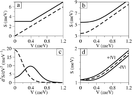
Figure 2: Current noise in a two terminal conductor vs. applied bias voltage for a spin accumulation of $\delta\mu=400$ $\mu$eV in a single lead (solid lines) or no spin accumulation in either lead (dashed lines). (a) $T=0$ K and $N=10$. (b) $T=1$ K and $N=10$. (c) Second derivative of the data in panel (b). (d) Typical asymmetry in the current noise as a function of applied bias for $T=1$ K and $N=2$.

For zero applied voltage, $V=0$, we get

$$\begin{split}\langle{S}\rangle=&(11/4)Nk_{\rm B}T+(1/4)N\delta\mu\\ &\times\left[2\coth(\delta\mu/2k_{\rm B}T)+\coth(\delta\mu/k_{\rm B}T)\right]\,.\end{split}$$ (11)

In the low temperature limit, $k_{\rm B}T\ll|\delta\mu|$, the noise due to the spin accumulation decouples from the thermal noise, allowing for the measurement of $\delta\mu$ by varying the temperature. In the opposite limit, $k_{\rm B}T\gg|\delta\mu|$, we recover the standard result for the Johnson-Nyquist noise, $S=4k_{\rm B}TG$.

So far we have shown how a spin accumulation can be quantitatively extracted from the ensemble averaged current noise. According to Eq. (7), the average $\langle{\cal T}_{\,\rm LR\rm RR}^{z0}\rangle$ vanishes. However, individual samples might exhibit a nonzero ${\cal T}_{\,\rm LR\rm RR}^{z0}$, which, quite importantly, generates a contribution to the noise that is antisymmetric in the bias voltage. Using Eq. (Measuring Spin Accumulations with Current Noise) we get, at zero temperature,

$$\delta S\equiv{S}(V)-{S}(-V)=2\,{\cal T}_{\,\rm LR\rm RR}^{z0}\big{\{}|eV+\delta\mu|-|eV-\delta\mu|\big{\}}\,,$$ (12)

while at high temperature the effect is washed out, as expected: $\delta S(V)=4/3\times T^{z0}_{\rm LRRR}\times\delta\mu\,{\rm e}V/k_{\rm B}T$.

We estimate the magnitude of this asymmetry in a typical mesoscopic sample by calculating the root mean square of ${\cal T}_{\,\gamma\delta\alpha\beta}^{z0}$. Again, using the method of Ref. Bro96 , we find that in chaotic ballistic systems

$$\langle{\rm var}\,{\cal T}_{\,\rm LR\rm RR}^{z0}\rangle_{\rm chaotic}=1/128+{\cal O}(N_{\rm T}^{-1})\,.$$ (13)

Accordingly, one has a typical asymmetry of $\delta S_{\rm typ}={\rm rms}(\delta S)=|eV|/2\sqrt{2}$ at low voltages and $\delta S_{\rm typ}=|\delta\mu|/2\sqrt{2}$ at higher voltages. This typical noise asymmetry is illustrated in Fig. 2(d). Interestingly, the asymmetry renders the noise smaller at finite voltage than at $V=0$. A noise asymmetry was reported in Ref. heidi in systems with broken time-reversal symmetry in the nonlinear regime. The mechanism for this asymmetry is, however, different here.

Because the asymmetry does not scale with the number of channels, while the total noise does, we predict that it is more evident in systems with few channels. The next order contributions tend to somewhat reduce the leading order result in Eq. (13). This is most pronounced at $N=1$, where time-reversal symmetry requires that ${\cal T}_{\,\rm LR\rm RR}^{z0}$ vanish identically. This is analogous to the vanishing of $\text{Tr}\left[\left(\mathbb{1}_{\beta}\otimes\sigma_{\beta}^{a}\right)s_{\alpha\beta}^{\dagger}s_{\alpha\beta}\right]$ found in Ref. kis . Our calculations therefore suggest that the asymmetry is best visible for $N=2$.

The method of Ref. Bro96 can also be applied to diffusive systems with an elastic mean free path much smaller than the linear system size, $\ell\ll L$. One obtains

$$\langle{\cal T}_{\,\rm LL\rm RR}^{ab}\rangle_{\rm diffusive} = \delta_{ab}\delta_{a0}(4/3)N\ell/L\,,$$ (14)

$$\langle{\cal T}_{\,\rm LR\rm RR}^{00}\rangle_{\rm diffusive} = (2/3)N\ell/L\,,$$ (15)

$$\langle{\rm var}\,{\cal T}_{\,\rm LR\rm RR}^{z0}\rangle_{\rm diffusive} = (2/35)\ell/L\,.$$ (16)

This gives, in particular, for $T=0$

$$\langle{S}\rangle=(2N\ell/3L)\left(|eV+\delta\mu|+|eV-\delta\mu|+2|\delta\mu|\right)\;,$$ (17)

and for $V=0$

$$\begin{split}\langle{S}\rangle=&(4N\ell/3L)\{3k_{\rm B}T+\delta\mu\\ &\times\left[\coth(\delta\mu/2k_{\rm B}T)+\coth(\delta\mu/k_{\rm B}T)\right]\}\,.\end{split}$$ (18)

Comparing Eqs. (10) and (11) with Eqs. (17) and (18) we see that after the substitution $N\to N\ell/L$, the noise averages for chaotic and diffusive conductors differ only by prefactors of order one.

With the above results, we now evaluate the ratio of a typical noise asymmetry to the ensemble averaged noise. At $|eV|=|\delta\mu|$, where this ratio is maximal, we get, at zero temperature,

$$\delta S_{\rm typ}/\langle S\rangle=(1/N)\times\left\{\begin{array}[]{ll}\sqrt{2}/3\,,&{\rm chaotic}\,,\\ \sqrt{9L/70\ell}\,,&{\rm diffusive}\,.\end{array}\right.\\ \,$$ (19)

Because metallic diffusive wires have $N\gg L/\ell$, we see that a chaotic system is better suited for detection of spin accumulation from the noise asymmetry.

We finally comment on the case of a spin dependent number of channels, $N_{\alpha\uparrow}\neq N_{\alpha\downarrow}$, which occurs for large enough spin accumulations, $\delta\mu_{\alpha}/\mu_{\alpha}>1/N_{\alpha}$ and breaks time-reversal symmetry. Equation (7) becomes

$$\begin{split}\langle{\cal T}_{\,\gamma\delta\alpha\beta}^{ab}\rangle=&N_{\alpha}^{0}N_{\beta}^{0}(N_{\rm T}^{0})^{-2}\,\left\{N_{\gamma}^{a}N_{\delta}^{b}\left(\frac{\delta_{\alpha\beta}}{N_{\alpha}^{0}}-\frac{1}{N_{T}^{0}}\right)\right.\\ &\left.+\delta_{\gamma\delta}\left[N_{\gamma}^{0}\delta_{ab}+N_{\gamma}^{z}(1-\delta_{ab})\right]\right\}\,,\end{split}$$ (20)

with $N^{0/z}_{\gamma}=N_{\gamma\uparrow}\pm N_{\gamma\downarrow}$. Interestingly, Eq. (20) implies a finite average asymmetry $\langle\delta S\rangle={\cal O}(N_{\gamma}^{z})$.

In our derivation of Eq. (Measuring Spin Accumulations with Current Noise), we neglected the energy dependence of the scattering matrix. This is legitimate as long as the expression in brackets in Eq. (1) is finite only in a narrow energy range. When this is not the case, the noise asymmetry will be damped even in individual samples $\delta S_{\rm typ}\rightarrow 0$, unless the spin accumulation is large enough that $N_{\rm L\uparrow}\neq N_{\rm L\downarrow}$. Simultaneously, Eq. (Measuring Spin Accumulations with Current Noise) may still give $\langle S\rangle$ provided one substitutes ${\cal T}\to\langle{\cal T}\rangle$. This is legitimate as long as the response is linear, meaning the applied voltages do not change the electrostatic profile of the conductor, and no substantial energy relaxation takes place in the system. We finally note that, in presence of dephasing, the noise asymmetry determined by Eq. (13) is algebraically damped, in the same way as conductance fluctuations are.wht We thus believe that the noise asymmetry we predict is observable even when dephasing is taken into account.

We thank Markus Büttiker and Eugene Mishchenko for interesting discussions. This work has been supported by NSF under Grant DMR-0706319.

References

(1) Ya.M. Blanter and M. Büttiker, Phys. Rep. 336,
1 (2000).
(2) C.W.J. Beenakker and C. Schönenberger,
Physics Today 56(5), 37 (2003).
(3) M. Reznikov, E. de-Picciotto, M. Heiblum, D.C. Glattli,
A. Kumar, and L. Saminadayar, Superlatt. Microstruct. 23, 901 (1998).
(4) Y.K. Kato, R.C. Myers, A.C. Gossard, and D.D. Awschalom,
Science 306, 1910 (2004).
(5) J. Wunderlich, B. Kästner, J. Sinova, and T. Jungwirth,
Phys. Rev. Lett. 94, 047204 (2005).
(6) E. Saitoh, M. Ueda, H. Miyajima, and G. Tatara,
Appl. Phys. Lett. 88, 182509 (2006)
(7) S.O. Valenzuela and M. Tinkham, Nature 442, 176 (2006).
(8) T. Kimura, Y. Otani, T. Sato, S. Takahashi, and S. Maekawa,
Phys. Rev. Lett. 98, 156601 (2007); ibid98,
249901(E) (2007).
(9) S.I. Erlingsson and D. Loss, Phys. Rev. B 72,
121310(R) (2005).
(10) Y. Tserkovnyak and A. Brataas, Phys. Rev. B 64,
214402 (2001).
(11) E.G. Mishchenko, Phys. Rev. B 68, 100409(R) (2003).
(12) A. Lamacraft, Phys. Rev. B 69, 081301(R) (2004).
(13) W. Belzig and M. Zareyan, Phys. Rev. B 69, 140407(R) (2004); M. Zareyan and W. Belzig, Europhys. Lett. 70, 817 (2005)
(14) K.E. Nagaev and L.I. Glazman, Phys. Rev. B 73, 054423 (2006).
(15) R.L. Dragomirova and B.K. Nikolic̀, Phys. Rev. B 75,
085328 (2007); R.L. Dragomirova, L.P. Zrbo, and B.K. Nikolic̀,
Europhys. Lett. 84, 37004 (2008).
(16) A. Cottet, W. Belzig, and C. Bruder, Phys. Rev. Lett. 92, 206801 (2004).
(17) J.H. Bardarson, İ. Adagideli and Ph. Jacquod,
Phys. Rev. Lett. 98, 196601 (2007); İ. Adagideli, J.H. Bardarson, and
Ph. Jacquod, J. Phys.: Condens. Matter 21, 155503 (2009).
(18)
P.W. Brouwer and C.W.J. Beenakker, J. Math. Phys. 37, 4904 (1996).
(19) R.S. Whitney and Ph. Jacquod,
Phys. Rev. Lett. 96, 206804 (2006).
(20) M.L. Mehta, Random Matrices, 2nd Ed.,
Academic Press (San Diego, 1991).
(21) A. A. Kiselev and K. W. Kim, Phys. Rev. B, 71 153315 (2005);F. Zhai and H.Q. Xu, Phys. Rev. Lett. 94, 246601 (2005).
(22) H. Förster and M. Büttiker, in AIP Conference Proceedings 1129, Twentieth International Conference on Noise edited by M. Macucci and G. Basso (Melville, New York, 2009).
(23) R. S. Whitney, Ph. Jacquod and C. Petitjean, Phys. Rev. B, 77, 045315 (2008).