Thermodynamics, spin-charge separation and correlation functions of spin-$1/2$ fermions with repulsive interaction

Abstract

We investigate the low temperature thermodynamics and correlation functions of one-dimensional spin-1/2 fermions with strong repulsion in an external magnetic field via the thermodynamic Bethe ansatz method. The exact thermodynamics of the model in a weak magnetic field is derived with the help of Wiener-Hopf techniques. It turns out that the low energy physics can be described by spin-charge separated conformal field theories of an effective Tomonaga-Luttinger liquid and an antiferromagnetic $SU(2)$ Heisenberg spin chain. However, these two types of conformally invariant low-lying excitations may break down as excitations take place far away from the Fermi points. The long distance asymptotics of the correlation functions and the critical exponents for the model in the presence of a magnetic field at zero temperature are derived in detail by solving dressed charge equations and by conformal mapping. Furthermore, we calculate the conformal dimensions for particular cases of correlation functions. The leading terms of these correlation functions are given explicitly for a weak magnetic field $H\ll 1$ and for a magnetic field close to the critical field $H\rightarrow H_{c}$. Our analytical results provide insights into universal thermodynamics and criticality in one-dimensional many-body physics.

I Introduction

Since the pioneering work in the 60’s, 70’s and 80’s by McGuire, Yang, Lieb, Sutherland, Baxter et al., and of the St Petersburg and Kyoto schools, the study of integrable models has flourished into a major activity. Almost without exception, the energy levels are given exactly in terms of the Bethe ansatz (BA) equations, from which physical properties can be calculated. This is a hallmark of integrable models that exhibit Yang-Baxter symmetry Bethe1931 . The knowledge and understanding gained from integrable models have greatly enhanced progress in the theory of phase transitions and critical phenomena. The most significant results achieved to date have been for two-dimensional lattice models and their related one-dimensional (1D) quantum spin chains as well as strongly correlated electronic systems book1 ; tak ; book2 ; book3 ; book4 . Integrable models are also known for systems such as Bose-Einstein condensates ZJMG ; Cao , metallic nanograins Siera and impurity models Konik ; Mehta2006 .

In general, the BA solution for 1D integrable systems is a set of coupled algebraic equations. Finding a set of solutions of quasimomenta and spin rapidities $\{k_{j},\Lambda_{j}\}$ for the BA equations gives the energy $\sum_{j}k_{j}^{2}$ and the momentum $\sum_{j}k_{j}$ of the system. However, the BA equations by themselves do not explicitly exhibit any temperature dependence. At zero temperature, the BA equations in principle give the complete eigenstates of the model. However, at finite temperatures, the equilibrium states become degenerate. Thus the thermodynamics of these BA solvable models are instead determined by a set of coupled nonlinear integral equations called the thermodynamic Bethe ansatz (TBA) equations Yang1969 . The TBA equations are expressed in terms of the dressed energies of different “Fermi seas” that are functions of temperature, chemical potential and external magnetic fields. The TBA equations in the zero temperature limit, i.e., $T\to 0$, give rise to the so called dressed energy equations which describe the band fillings with respect to Zeeman fields and chemical potentials.

The TBA equations are very difficult to solve in general. They involve an infinite number of coupled nonlinear integral equations for spin strings which are quite cumbersome to solve using either analytical or numerical methods tak ; book3 . Recently, Caux et al Caux1 ; Caux2 developed numerical schemes to solve the TBA equations of the 1D two-component spinor Bose gas with delta-function interaction. The results obtained by these numerical schemes show an insightful interplay between quantum statistics, interactions and temperature in 1D interacting many-body systems. In the context of the quantum transfer matrix method QTM , Klümper and Patu Klumper derived the nonlinear integral equations for the 1D Bose and Fermi gases with repulsive delta-function interaction. This approach opens up the possibility of obtaining the thermodynamics of the continuum models of interacting fermions and bosons by taking an appropriate limit for the integrable lattice models. The advance of such approaches is the reduction of the infinite number of TBA equations to a finite number of the nonlinear integral equations. Where the finite number of the nonlinear integral equations for the lattice models can be solved numerically and analytically in certain temperature regimes BGOT ; T-system . Despite giving high precision numerical thermodynamics, finding the universal nature of interacting particles requires further analytical input. Significant universal features of 1D many-body systems are Tomonaga-Luttinger liquid physics and quantum critical phenomena at low temperatures which involve finding essentially universal parameters such as central charges, Luttinger parameters, correlation exponents and dynamical critical exponents. All studies of these universal parameters call for mathematical analysis and analytical derivation.

Some progress has been made to derive low temperature analytic results for BA solvable models. For example, Mezincescu et al. Nepomechie1992 ; Nepomechie1993 obtained the free energy of spin chains at low temperatures under a small magnetic field by using the Wiener-Hopf technique. Johnson and McCoy Johnson1972 obtained the leading temperature dependent terms in a low temperature expansion of the free energy for the massive regime of the Heisenberg model. Filyov et al. Filyov1981 gave an exact solution to the s-d exchange model expressed as a series in terms of the temperature. Some analytical results for the TBA equations of 1D many-body systems are restricted to the ground state ($T=0$) in the strong coupling limit ($c\gg 1$) Penc ; GB ; Wadati . Recently, further progress has been made to obtain the analytic finite temperature thermodynamics and quantum criticality of 1D attractive fermions with strongly attractive interactions Zhao2009 ; Guan2010 ; GHo ; GBat .

(1+1)-dimensional critical systems not only have global scale invariance but exhibit local scale invariance (conformal invariance) too. The conformal group in (1+1)-dimensions is infinite dimensional and completely determines the critical exponents and bulk correlation functions at criticality for gapless excitations Belavin1984 . Close to criticality, the dispersion relations for 1D quantum systems are approximately linear. Conformal invariance predicts that the energy per unit length has a universal finite size scaling form $E=E_{0}+\Delta/L^{2}$ where $E_{0}$ is the ground state energy per unit length for the infinite system and $\Delta$ is a universal term. These universality classes are characterized by the dimensionless number $C$ (contained in the term $\Delta$) which is the central charge of the underlying Virasoro algebra Affleck1986 ; Blote1986 . Affleck Affleck1986 also showed that conformal invariance gives a universal form for the finite temperature effects on the free energy by replacing $1/L$ with $T$ in the conformal map $z=\exp(2\pi\omega/L)$. At the same time, Cardy Cardy1986 showed that the two-point correlation function between primary fields can be directly derived from conformal mapping using transfer matrix techniques and expressed the conformal dimensions in terms of finite-size corrections to the energy spectrum. When $C<1$, it takes on discrete values only i.e., $C$ is quantized and hence the conformal dimensions are restricted to certain rational numbers Friedan1984 . On the other hand when $C\geq 1$, the critical exponents may depend continuously on the parameters of the model Zamolodchikov1985 .

The critical exponents for BA integrable models can be calculated via the quantum inverse scattering method (QISM) in terms of a function $Z(\lambda)$ called the dressed charge. In this way Bogoliubov et al. Bogoliubov1986 obtained explicit expressions for the correlation functions for the Bose gas and the XXX and XXZ chains. Izergin et al. Izergin1989 considered the finite-size corrections to multicomponent BA systems and presented a formula for the dressed charge matrix $Z_{\alpha\beta}$ which determines the critical exponents. They also showed that the integral equations for the dressed charge matrix depend only on the quantum $R$-matrix of the model, which means that the universal class of critical exponents are described by the $R$-matrix and the structure of the ground states of the integrable models. This universality property is a consequence of conformal invariance. Other models like the impenetrable Bose gas Its1990 , the supersymmetric $t-J$ model Kawakami1991 and the Hubbard model Frahm1990 ; Frahm1991 ; Woynarovich1987 ; Woynarovich1989 have also been considered in the context of the QISM approach. The Luttinger liquid is an alternative approach based on the fact that these models are certain realizations of the Gaussian model Haldane1981a ; Haldane1981b . Progress has also been made using Fredholm determinant representations of time-dependent temperature correlation functions for bosons and fermions in 1D when $c=\infty$ Izergin1997 ; Izergin1998 .

In this paper, we focus on the universal nature of 1D repulsive spin-1/2 fermions in the frame work of the TBA formalism, including Luttinger physics and critical behaviour of correlation functions. In order to elucidate the significant features of spin-charge separation and critical exponents at quantum criticality, it is essential to analytically calculate the dressed energy potentials which encode the quantum and thermal fluctuations of the spin and charge degrees of freedom in the critical regime. We investigate the low temperature thermodynamics of strongly repulsive spin-1/2 fermions in a small magnetic field and a magnetic field close to the saturation field via the TBA method. We take an approximation to the TBA equations in the strong coupling regime, where the interacting strength $c\gg 1$. Thus the TBA equations are transformed into a new set of equations which can be solved using the Wiener-Hopf method. A comparison of the pressure and the entropy is made between the application of two different integral expansions. These are Sommerfeld’s lemma, which is valid for very low temperatures, and the polylogarithm function which is valid for finite temperatures. The result from Sommerfeld expansion agrees with the conformal field theory prediction Affleck1986 ; Blote1986 . It is shown that the low energy physics can be described by a spin-charge separated theory of an effective Tomonaga-Luttinger liquid and antiferromagnetic $SU(2)$ Heisenberg spin chain. A universal crossover from a relativistic dispersion to a nonrelativistic dispersion is determined by the exact thermodynamics extracted from the polylogarithm function. We also derive the explicit dressed charge matrix elements for the model in a weak external field $H\ll 1$ using the Wiener-Hopf method again, and also for the case that is close to the ferromagnetic state $H\rightarrow H_{c}$, where $H_{c}$ is the critical magnetic field. Various two-point and multi-point correlation functions at zero temperature are derived based on the expressions obtained from the dressed charge matrix. The leading terms and their critical exponents are given explicitly. Our results show that there is indeed no long-range order in this system.

The spin-1/2 fermion model under consideration is the continuum limit of the 1D Hubbard model (see, e.g., pp 45-49 of Ref. book3 ), which has been widely studied book3 . In particular, the various correlation functions and scaling dimensions obtained here for the spin-1/2 fermion model have been derived for the 1D Hubbard model, for interacting fermions and for a mixture of bosons and fermions using the dressed charge formalism book3 ; Frahm1990 ; Frahm1991 ; Frahm-P ; Lee-Guan . Accordingly our results in the infinite coupling limit reduce to those obtained for the 1D Hubbard model with an infinitely strong repulsion. Caution should be paid to the order of the limits $T\to 0$ and infinite strong coupling Cheianov . Taking the $T\to 0$ limit first, the correlations (for example, the one-particle correlation) show the scaling behavior of conformal field theory in the infinite strong coupling limit. However, taking the infinite strong coupling limit first, the correlations decay exponentially in the $T\to 0$ limit. The two limits do not commute. Moreover, in the grand canonical ensemble, the Tomonaga-Luttinger liquid exists only in a certain region where the chemical potential is greater than the critical value. Below the critical chemical potential, the low temperature thermodynamics is that of an ideal gas in another regime, see Gohmann .

The corrections we have obtained in terms of strong but finite coupling are of importance because of the experimental developments which enable access to the finitely strong coupling regime nature . Our analytical $1/c$ order corrections to the critical exponents indicate an important signature – the critical exponents depend on the model parameters with central charge $C\geq 1$. In addition, our thermodynamical properties are valid for temperatures from $T=0$ to $T\ll c^{2}$. Results of this kind are necessary to test critical phenomena and spin-charge separation theory in experiments with trapped fermionic atoms. Indeed, along with extending the known results for the thermodynamics and correlations, this is our main motivation here.

This paper is set out as follows. In Section II we introduce the model and present the TBA equations. The low temperature thermodynamics is derived in Section III by expressing the TBA equations in the form of Wiener-Hopf integral equations. We solve the dressed charge equations for the model in the small field limit ($H\ll 1$) and in the limit where the field approaches the critical value ($H\rightarrow H_{c}$) in Section IV. In Section V, we calculate the correlation functions of various operators in both limits. We then give a summary of our main results and concluding remarks in Section VI. Some detailed working and results are given in the Appendices. In Appendix A, we derive the ground state thermodynamics and the critical field for the model. The Wiener-Hopf method is discussed in Appendix B. A more detailed derivation of the low temperature thermodynamics is given in Appendix C. The leading terms of the zero temperature correlation functions are given in Appendices D and D.

II The TBA equations

We consider a system of 1D spin-1/2 fermions with delta-function interaction, with hamiltonian

$$\mathscr{H}=\mathscr{H}_{0}-\mu N,\qquad\mathscr{H}_{0}=-\sum_{j=1}^{N}\frac{\partial}{\partial x_{j}^{2}}+2c\sum_{1\leq j<k\leq N}\delta(x_{j}-x_{k})-HM.$$ (1)

Here $N=N_{\uparrow}+N_{\downarrow}$ is the total number of spin-up $N_{\uparrow}$ and spin-down $N_{\downarrow}$ fermions and $M=(N_{\uparrow}-N_{\downarrow})/2$ is the magnetization. $\mu$ and $H$ are the chemical potential and the magnetic field. In this paper, we exclusively consider the case of repulsive interaction for which $c>0$.

The ground state properties can be obtained using the BA solution Yang ; Gaudin (see Appendix A for a brief review). On the other hand, at finite temperatures $T>0$, the physical quantities are described by the following set of non-linear integral equations, which are referred to as the TBA equations tak ; Lai . In the thermodynamic limit, their explicit form is

$$\varepsilon(k) =k^{2}-\mu-\frac{H}{2}-T\sum_{n=1}^{\infty}a_{n}\ast\ln\left(1+e^{-\phi_{n}(k)/T}\right)$$ (2)

$$\phi_{n}(\lambda) =nH-Ta_{n}\ast\ln\left(1+e^{-\varepsilon(\lambda)/T}\right)+T\sum_{m=1}^{\infty}T_{nm}\ast\ln\left(1+e^{-\phi_{m}(\lambda)/T}\right)$$ (3)

or equivalently

$$\varepsilon(k) =k^{2}-\mu-TK\ast\ln(1+e^{-\varepsilon(k)/T})-Ts\ast\ln\left(1+e^{\phi_{1}(k)/T}\right)$$ (4)

$$\phi_{1}(\lambda) =Ts\ast\ln\left(1+e^{\phi_{2}(\lambda)/T}\right)-Ts\ast\ln\left(1+e^{-\varepsilon(\lambda)/T}\right)$$ (5)

$$\phi_{n}(\lambda) =Ts\ast\ln\left(1+e^{\phi_{n-1}(\lambda)/T}\right)+Ts\ast\ln\left(1+e^{\phi_{n+1}(\lambda)/T}\right)$$ (6)

where the functions $\phi_{n}(\lambda)$ must satisfy the condition

$$\lim_{n\rightarrow\infty}\frac{\phi_{n}(\lambda)}{n}=H.$$ (7)

The functions $a=a_{n}(\lambda)$, $s=s(\lambda)$, $K=K(\lambda)$ and $T_{nm}=T_{nm}(\lambda)$ are defined by

$$a_{n}(\lambda)=\frac{1}{\pi}\frac{nc/2}{(nc)^{2}/4+\lambda^{2}},\quad s(\lambda)=\frac{1}{2c\cosh(\pi\lambda/c)},\quad K(\lambda)=\frac{1}{2\pi}\int_{-\infty}^{\infty}\frac{1}{1+e^{c|\omega|}}e^{-i\omega\lambda}d\omega,$$

$$T_{nm}(\lambda)=\begin{cases}a_{|n-m|}(\lambda)+2a_{|n-m|+2}(\lambda)+\ldots+2a_{n+m-2}(\lambda)+a_{n+m}(\lambda)&\text{ for $n\neq m$};\\ 2a_{2}(\lambda)+2a_{4}(\lambda)+\ldots+2a_{2n-2}(\lambda)+a_{2n}(\lambda)&\text{ for $n=m$}.\end{cases}$$ (8)

The asterisk $*$ denotes the convolution $f\ast g(x)=\int_{-\infty}^{\infty}f(x-x^{\prime})g(x^{\prime})dx^{\prime}$.

The bulk quantities are characterized by the solution to the TBA equations. For instance, the free energy per unit length $F$ and the pressure $P$ are given by

$$F=\mu n_{c}-P,\qquad P=\frac{T}{2\pi}\int_{-\infty}^{\infty}\ln(1+e^{-\varepsilon(k)/T})dk,$$ (9)

where $n_{c}$ denotes the particle density.

III Low-temperature thermodynamics

The most complicated part of the TBA equations is the string part (which characterizes the spin excitations) consisting of an infinite number of string functions $\phi_{n}(\lambda)$ ((3) or (5) and (6)). These coupled nonlinear integral equations have not been solved in the most generic manner, but the obstacles can be overcome if we make certain assumptions for the parameters involved. Among them, one of the most crucial cases which we consider below, is the low-temperature limit $T\ll 1$. In this limit, the TBA equations reduce to a set of linearly coupled equations, which are easier to deal with. Moreover for the strong coupling regime $c\gg 1$ in a weak magnetic field $H\ll 1$, we can solve the linear integral equations analytically. Below we derive the analytical solutions in this physical regime: strong coupling $c\gg 1$, weak magnetic field $H\ll 1$ and low-temperature $T\ll 1$. The low-temperature thermodynamics for the generic case of $c>0$ and $H\leq H_{c}$ ($H_{c}$ is the critical field) is derived in Appendix C.

We first observe from equation (6) that $\phi_{n}(\lambda)>0$ for $n>1$, because $s(\lambda)>0$ and $\ln(1+e^{\phi_{n}(\lambda)/T})>0$ for $\lambda\in\mathbb{R}$ and $n\geq 1$. This positivity condition implies that the function $T\ln(1+e^{-\phi_{n}(\lambda)/T})\rightarrow 0$ for $T\rightarrow 0$ and $n>1$. Therefore, in the low temperature limit $T\ll 1$, all the higher spin string functions drop off leaving only the function $\phi_{1}(\lambda)$ in the first set of TBA equations. The revised form is

$$\varepsilon(k) =k^{2}-\mu-\frac{H}{2}-Ta_{1}\ast\ln(1+e^{-\phi_{1}(k)/T})$$ (10)

$$\phi_{1}(\lambda) =H-Ta_{1}\ast\ln(1+e^{-\varepsilon(\lambda)/T})+Ta_{2}\ast\ln(1+e^{-\phi_{1}(\lambda)/T}).$$ (11)

We now have to solve two coupled integral equations with only two unknown functions $\varepsilon(k)$ and $\phi_{1}(\lambda)$. Let us analyze them in the strong coupling regime $c\gg 1$, where the above equations are further simplified. Analyzing the dispersion $\varepsilon(k)$, we are able to rewrite the term GBT

$$Ta_{1}\ast\ln\left(1+e^{-\varepsilon(\lambda)/T}\right)\approx 2\pi Pa_{1}(\lambda)+O\left(\frac{1}{c^{3}}\right),$$ (12)

where the major contribution to the integral comes from a finite range $(-k_{0},k_{0})$. As shown in Appendix A, one notices that the points $\pm k_{0}$ correspond to the Fermi points in the charge Fermi sea. Thus equation (11) simplifies to

$$\phi_{1}(\lambda)=H-2\pi Pa_{1}(\lambda)+Ta_{2}\ast\ln\left(1+e^{-\phi_{1}(\lambda)/T}\right).$$ (13)

Using the Fourier transform, this equation and Eq. (10) can also be expressed as

$$\varepsilon(k)=k^{2}-\mu-2\pi PK(k)-Ts\ast\ln(1+e^{\phi_{1}(k)/T})$$

$$\phi_{1}(\lambda)=\frac{H}{2}-2\pi Ps(\lambda)+TK\ast\ln(1+e^{\phi_{1}(\lambda)/T}).$$ (14)

To proceed further, let us separate the function $\phi_{1}(\lambda)$ into two parts:

$$\phi_{1}(\lambda)=\phi_{1}^{(0)}(\lambda)+\phi_{1}^{(1)}(\lambda).$$ (15)

The first part $\phi_{1}^{(0)}(\lambda)$ corresponds to the leading order term when $T=0$, while the second part $\phi_{1}^{(1)}(\lambda)$ is the first order correction to the limit $T\to 0$. Analyzing the leading term $H/2-2\pi Ps(\lambda)$ in Eq. (14), we find that $\phi_{1}^{(0)}(\lambda)$ should satisfy the linear integral equation

$$\phi^{(0)}_{1}(\lambda)=\frac{H}{2}-2\pi P_{0}s(\lambda)+K\ast\phi_{1}^{(0)+}(\lambda)$$ (16)

where $P_{0}$ denotes the pressure at $T=0$. Here we have divided $\phi_{1}^{(0)}(\lambda)$ into its positive and negative parts:

$$\phi_{1}^{(0)}(\lambda)=\phi_{1}^{(0)+}(\lambda)+\phi_{1}^{(0)-}(\lambda),$$

$$\phi_{1}^{(0)-}(\lambda)=\begin{cases}\phi_{1}^{(0)}(\lambda)&\text{ for $|\lambda|\leq\lambda_{0}$}\\ 0&\text{ for $|\lambda|>\lambda_{0}$}\end{cases}.$$ (17)

Note that the function $\phi_{1}^{(0)}(\lambda)$ is nothing but the dressed energy $\varepsilon_{s}(\lambda)$ (106) denoting the energy of a spinon excitation with rapidity $\lambda$, and the points $\pm\lambda_{0}$ are the Fermi points (see Appendix A for details). On the other hand, the function $\varepsilon(k)$ at $T=0$ corresponds to the dressed energy $\varepsilon_{c}(k)$ (106) describing the energy of charge excitation with momentum $k$.

Substituting Eq. (15) into Eq. (14), and subtracting Eq. (16) from the resulting equation gives

$$\phi_{1}^{(1)}(\lambda) =-2\pi(P-P_{0})s(\lambda)+\int_{|\mu|\geq\lambda_{0}}K(\lambda-\mu)\left(T\ln\left(1+e^{(\phi_{1}^{(0)}(\mu)+\phi_{1}^{(1)}(\mu))/T}\right)-\phi_{1}^{(0)+}(\mu)\right)d\mu$$

$$\quad+\int_{|\mu|\leq\lambda_{0}}TK(\lambda-\mu)\ln\left(1+e^{(\phi_{1}^{(0)}(\mu)+\phi_{1}^{(1)}(\mu))/T}\right)d\mu.$$ (18)

An iteration procedure shows that $\phi_{1}^{(1)}(\lambda)=o(T)$. Thus one sees that

$$\phi_{1}^{(1)}(\lambda)\approx-2\pi(P-P_{0})s(\lambda)+E_{K}(\lambda)+\int_{|\mu|\geq\lambda_{0}}K(\lambda-\mu)\phi_{1}^{(1)}(\mu)d\mu$$ (19)

where we denote

$$E_{K}(\lambda)=TK\ast\ln\left(1+e^{-|\phi_{1}^{(0)}(\lambda)|/T}\right).$$ (20)

In the limit $T\to 0$, the major contributions towards $E_{K}(\lambda)$ come from the regions near $\pm\lambda_{0}$. Hence we expand $\phi_{1}^{(0)}(\lambda)$ around $\lambda=\pm\lambda_{0}$

$$\phi_{1}^{(0)}(\lambda)=t(\lambda-\lambda_{0})+O((\lambda-\lambda_{0})^{2})$$ (21)

where $t\equiv\left.d\phi_{1}^{(0)}(\lambda)/d\lambda\right|_{\lambda=\lambda_{0}}$. Then we find

$$E_{K}(\lambda) \approx T\int_{|\mu-\lambda_{0}|<\epsilon}K(\lambda-\mu)\ln(1+e^{-t|\mu-\lambda_{0}|/T})d\mu$$

$$\approx\frac{2T^{2}}{t}[K(\lambda-\lambda_{0})+K(\lambda+\lambda_{0})]\int_{0}^{\infty}\ln\left(1+e^{-u}\right)du$$

$$=\frac{\pi^{2}T^{2}}{6t}[K(\lambda-\lambda_{0})+K(\lambda+\lambda_{0})].$$ (22)

Therefore we obtain a linear integral equation which determines $\phi_{1}^{(1)}(\lambda)$, namely

$$\phi_{1}^{(1)}(\lambda)\approx-2\pi(P-P_{0})s(\lambda)+\frac{\pi^{2}T^{2}}{6t}[K(\lambda-\lambda_{0})+K(\lambda+\lambda_{0})]+\int_{|\mu|\geq\lambda_{0}}K(\lambda-\mu)\phi_{1}^{(1)}(\mu)d\mu.$$ (23)

In completely the same way, one finds that the low temperature behavior of $\varepsilon(k)$ (14) is described by

$$\varepsilon(k)\approx k^{2}-\mu-2\pi PK(k)-\frac{\pi^{2}T^{2}}{6t}[s(k-\lambda_{0})+s(k+\lambda_{0})]-\int_{|\lambda|\geq\lambda_{0}}s(k-\lambda)\left[\phi_{1}^{(0)}(\lambda)+\phi_{1}^{(1)}(\lambda)\right]d\lambda.$$ (24)

Eq. (16) and Eq. (23) can be solved for $H\ll 1$ via the Wiener-Hopf technique as in Nepomechie1992 ; Nepomechie1993 ; book3 . For convenience, let us introduce the functions

$$y^{(k)}(\lambda):=\phi_{1}^{(k)}(\lambda+\lambda_{0})\qquad(k=0,1).$$ (25)

By definition (see Eq. (17)), the Fermi points $\pm\lambda_{0}$ are determined by the condition

$$\phi_{1}^{(0)}(\lambda_{0})=y^{(0)}(0)=0.$$ (26)

Applying the iterative procedure to Eq. (16), one sees $y^{(0)}(0)=0=H/2-2\pi P_{0}s(\lambda_{0})+O(H)$. Solving this equation, one finds that $\lambda_{0}\approx-\ln H$ for $H\ll 1$. Because $K(\lambda)$ rapidly decreases with $\lambda>0$, we may solve the integral equations (16) and (23) by expanding

$$y^{(k)}(\lambda)=\sum_{n=0}^{\infty}y^{(k)}_{n}(\lambda)\qquad(k=0,1).$$ (27)

$y_{n}^{(k)}(\lambda)$ obeys the integral equation

$$y_{n}^{(k)}(\lambda)=g^{(k)}_{n}(\lambda)+\int_{0}^{\infty}K(\lambda-\mu)y_{n}^{(k)}(\mu)d\mu$$ (28)

where the driving terms $g_{n}^{(0)}(\lambda)$ and $g_{n}^{(1)}(\lambda)$ in the limit of $T\ll 1$ are explicitly given by

$$g_{0}^{(0)}(\lambda)=\frac{H}{2}-2\pi P_{0}s(\lambda+\lambda_{0})\quad$$

$$g_{0}^{(1)}(\lambda)=-2\pi(P-P_{0})s(\lambda+\lambda_{0})+\frac{\pi^{2}T^{2}}{6t}K(\lambda)$$

$$g_{n}^{(k)}(\lambda)=\int_{0}^{\infty}K(\lambda+\mu+2\lambda_{0})y^{(k)}_{n-1}(\mu)d\mu\qquad(n\geq 1).$$ (29)

The above equations are the so-called Wiener-Hopf type integral equations. In Appendix B, a method to solve the Wiener-Hopf type integral equations is given. Let us decompose $\widehat{y}^{(k)}(\omega)$ into a sum of two parts, i.e., $\widehat{y}^{(k)}(\omega)=\widehat{y}^{(k)}_{+}(\omega)+\widehat{y}^{(k)}_{-}(\omega)$, where $\widehat{y}_{+}^{(k)}(\omega)$ ($\widehat{y}_{-}^{(k)}(\omega)$) is analytic in the upper (lower) half plane (see Eq. (114) in Appendix B). For the leading terms $\widehat{y}_{0}^{(k)}(\omega)$, we obtain (see Eqs (131) and (134))

$$\widehat{y}_{0+}^{(0)}(\omega)=G_{+}(\omega)\left[\frac{iHG_{-}(-i\epsilon)}{2(\omega+i\epsilon)}-\frac{2\pi iP_{0}}{c}\frac{G_{-}(-\pi i/c)e^{-\pi\lambda_{0}/c}}{\omega+\pi i/c}\right]+O(H^{2})$$

$$\widehat{y}_{0+}^{(1)}(\omega)=\frac{\pi^{2}T^{2}}{6t}(G_{+}(\omega)-1)-\frac{2\pi i(P-P_{0})}{c}\frac{G_{+}(\omega)G_{-}(-\pi i/c)e^{-\pi\lambda_{0}/c}}{\omega+\pi i/c}$$ (30)

where $G_{\pm}(\omega)$ is defined by Eq. (123). Using the formula as in (121), and combining the above equation with the condition (26), we determine the leading term of the Fermi points $\lambda_{0}$ to be

$$\lambda_{0}\approx\frac{c}{\pi}\ln\left(\frac{H_{0}}{H}\right),\qquad H_{0}=\frac{4\pi P_{0}G_{-}(-\pi i/c)}{cG_{-}(0)}=\frac{4\pi P_{0}}{c}\sqrt{\frac{\pi}{2e}}=\sqrt{\frac{\pi^{3}}{2e}}H_{c}+O\left(\frac{1}{c^{2}}\right)$$ (31)

where we have used the formulae (116) and (124). To derive the last equality in the second equation we used the property (see Appendix A)

$$\frac{P_{0}}{c}=-\frac{1}{2\pi c}\int_{-k_{0}}^{k_{0}}\varepsilon_{c}(k)dk\approx\frac{H_{c}}{4}+O\left(\frac{1}{c}\right)$$ (32)

where $H_{c}$ is the critical magnetic field, where all fermion spins point up (see Guan2008 or Eq. (111) in Appendix A), with $H_{c}\approx 8n_{c}^{3}\pi^{2}/3c$.

From the relation (25), the integral in (24) can be evaluated as follows:

$$\int_{|\lambda|\geq\lambda_{0}}s(k-\lambda)\phi_{1}^{(k)}(\lambda)d\lambda \approx\frac{2e^{-\frac{\pi}{c}\lambda_{0}}}{c}\int_{0}^{\infty}e^{-\frac{\pi}{c}\lambda}y_{0}^{(k)}(\lambda)d\lambda$$

$$=\frac{2e^{-\frac{\pi}{c}\lambda_{0}}}{c}\int_{0}^{\infty}e^{-\frac{\pi}{c}\lambda}d\lambda\int_{-\infty}^{\infty}\frac{d\omega}{2\pi}e^{-i\lambda\omega}\widehat{y}_{0+}^{(k)}(\omega)$$

$$=-\frac{ie^{-\frac{\pi}{c}\lambda_{0}}}{\pi c}\int_{-\infty}^{\infty}\frac{d\omega}{\omega-\pi i/c}\widehat{y}_{0+}^{(k)}(\omega)$$

$$=\frac{2e^{-\frac{\pi}{c}\lambda_{0}}}{c}\widehat{y}_{0+}^{(k)}\left(\frac{\pi i}{c}\right)$$ (33)

where the relation $s(k\pm|\lambda+\lambda_{0}|)\approx e^{-\pi(\lambda+\lambda_{0})/c}/c$ is used in the first line. Substitution of Eq. (33) together with Eqs. (31), (30) and (124) into Eq. (24) yields

$$\varepsilon(k)\approx k^{2}-\mu-2\pi PK(k)-\frac{cPH^{2}}{4\pi^{2}P_{0}^{2}}-\frac{\pi T^{2}H}{6\sqrt{2}P_{0}t}.$$ (34)

Inserting the relations

$$K(k)\approx\frac{\ln 2}{c\pi},\qquad t\approx y_{0}^{\prime}(0)=-\lim_{\omega\to\infty}\omega^{2}\widehat{y}_{0+}^{(0)}(\omega)=\frac{\pi H}{\sqrt{2}c}$$ (35)

and using $P\approx P_{0}$, we arrive at

$$\varepsilon(k)\approx k^{2}-\mu-\frac{2P\ln{2}}{c}-\frac{cH^{2}}{4\pi^{2}P}-\frac{cT^{2}}{6P}=k^{2}-A$$ (36)

where $A:=\mu+2P\ln 2/c+cH^{2}/4\pi^{2}P+cT^{2}/6P$. We would like to address that the calculation of the dressed energy potential (36) is essential for catching spin-charge separation signature and quantum criticality at low temperatures. The terms in the function $A$ show an important implementation of spin density and charge density fluctuations that reveals a physical origin of spin-charge separation. This is clearly seen from the following low temperature and finite temperature thermodynamics. In view of this validity of catching this universal nature, we see that the result (36) is also helpful to numerics. Using this function $A$, we then perform integration by parts on the pressure of the system (9) to get

$$P=\frac{1}{\pi}\int_{0}^{\infty}\frac{\sqrt{\varepsilon}d\varepsilon}{1+e^{(\varepsilon-A)/T}}=-\frac{1}{\sqrt{4\pi}}T^{\frac{3}{2}}\mathrm{Li}_{\frac{3}{2}}\left(-e^{A/T}\right)$$ (37)

where $\mathrm{Li}_{s}(z)$ is polylogarithm function defined by

$$\mathrm{Li}_{s}(z)=\sum_{k=1}^{\infty}\frac{z^{k}}{k^{s}}.$$ (38)

For fixed particle density, the chemical potential is determined by solving the equation $n_{c}=\partial P/\partial\mu$. By inserting Eq. (37) into Eq. (9), the low-temperature thermodynamics in the region $H\ll 1$ and $c\gg 1$ is completely determined. To capture universal features of the low-temperature thermodynamics, we further expand Eq. (37) by making use of Sommerfeld’s lemma (see Pathria ; GBT for instance):

$$P=\frac{2A^{3/2}}{3\pi}\left(1+\frac{\pi^{2}}{8}\left(\frac{T}{A}\right)^{2}+O(T^{4})\right).$$ (39)

Furthermore, we use the relation $n_{c}=\partial P/\partial\mu$ and repeatedly iterate the terms to eliminate those with orders higher than $T^{2}$, $H^{2}$ and $1/c$. After some lengthy algebra, we finally obtain the chemical potential

$$\mu\approx\pi^{2}n_{c}^{2}\left(1-\frac{16\ln 2}{3\gamma}\right)+\frac{3\gamma H^{2}}{4\pi^{4}n_{c}^{2}}\left(1+\frac{3\ln 2}{\gamma}\right)+\frac{\gamma T^{2}}{2\pi^{2}n_{c}^{2}}\left(1+\frac{3\ln 2}{\gamma}\right)+\frac{T^{2}}{12n_{c}^{2}}$$ (40)

where $\gamma$ denotes $\gamma:=c/n_{c}$. Substituting (40) into the expression for the pressure (39) and then iterating the pressure itself, we obtain

$$P\approx\frac{2}{3}\pi^{2}n_{c}^{3}\left(1-\frac{6\ln 2}{\gamma}\right)+\frac{9\gamma H^{2}}{8\pi^{4}n_{c}}\left(1+\frac{4\ln 2}{\gamma}\right)+\frac{3\gamma T^{2}}{4\pi^{2}n_{c}}\left(1+\frac{4\ln 2}{\gamma}\right)+\frac{T^{2}}{6n_{c}}.$$ (41)

The free energy of the system defined by Eq. (148) is given by

$$F\approx\frac{1}{3}\pi^{2}n_{c}^{3}\left(1-\frac{4\ln 2}{\gamma}\right)-\frac{3\gamma H^{2}}{8\pi^{4}n_{c}}\left(1+\frac{6\ln 2}{\gamma}\right)-\frac{\gamma T^{2}}{4\pi^{2}n_{c}}\left(1+\frac{6\ln 2}{\gamma}\right)-\frac{T^{2}}{12n_{c}}.$$ (42)

From this free energy (42), we have the susceptibility

$$\chi=-\frac{\partial^{2}F}{\partial H^{2}}\approx\frac{3\gamma}{4\pi^{4}n_{c}}\left(1+\frac{6\ln 2}{\gamma}\right).$$ (43)

This susceptibility can be possibly tested in an trapped 1D Fermi gas of cold atom. We rewrite the pressure (37)

$$p=-\sqrt{\frac{m}{2\pi\hbar^{2}}}T^{\frac{3}{2}}\mathrm{Li}_{\frac{3}{2}}\left(-e^{X}\right)$$ (44)

where

$$X = \frac{\mu}{T}-\frac{\ln 2}{\sqrt{\pi}}\sqrt{\frac{T}{\varepsilon_{0}}}\mathrm{Li}_{\frac{3}{2}}\left(-e^{\frac{\mu}{T}}\right)-\frac{1}{2\pi^{\frac{3}{2}}}\frac{H^{2}}{T^{2}}\frac{1}{\sqrt{\frac{T}{\varepsilon_{0}}}\mathrm{Li}_{\frac{3}{2}}\left(-e^{\frac{\mu}{T}}\right)}$$ (45)

$$-\frac{\sqrt{\pi}}{3}\frac{1}{\sqrt{\frac{T}{\varepsilon_{0}}}\mathrm{Li}_{\frac{3}{2}}\left(-e^{\frac{\mu}{T}}\right)}.$$

In dimensionless units, i.e. $h=H/\varepsilon_{0}$ and $\mu=\mu/\varepsilon_{0}$ with $\varepsilon_{0}=\frac{\hbar^{2}}{2m}c^{2}$, the susceptibility is given by

$$\frac{\chi}{\varepsilon_{0}}=\frac{c}{\varepsilon_{0}}\frac{3\gamma}{4\pi^{4}n^{\prime}(\mu,h)}\left(1+\frac{6\ln 2}{\gamma}\right).$$ (46)

which agrees with the field theory prediction $\chi v_{s}=\theta/\pi$. Here $\theta=1/2$. The holon velocity $v_{c}$ and spinon velocity $v_{s}$ at $H=0$ are given in (150) in Appendix C. In the above equation, the density is given by

$$n^{\prime}: = \frac{n}{\sqrt{\varepsilon_{0}}}\approx\frac{\mu}{\pi}\left[1-\frac{3}{8\pi\sqrt{\mu}}\left(\frac{h}{\mu}\right)^{2}\left(1+\frac{3\sqrt{\mu}\ln 2}{\pi}\right)+\frac{8\sqrt{\mu}\ln 2}{3\pi}\right]$$ (47)

and the dimensionless interaction strength is given by

$$\frac{1}{\gamma}\approx\frac{\sqrt{\mu}}{\pi}-\frac{3}{8\pi^{2}}\left(\frac{h}{\mu}\right)^{2}.$$ (48)

In Fig. 1, we plot the susceptibility for different values of the chemical potentials at low temperatures. In contrast, in Chapter 13 of Ref. book3 , the thermal and magnetic properties of the 1D Hubbard model are plotted by using the result obtained for the thermodynamics of the 1D Hubbard model by numerically solving nonlinear integral equations (NLIE). The thermodynamics for the Hubbard model can be calculated by the quantum transfer matrix method for all temperatures. Here we have obtained an explicit low temperature expansion for the fermion model. The result (44) for the pressure contains the spin density and charge thermal potentials at criticality and may thus possibly be used to test the spin and charge velocities in experiments with ultracold atomic fermions in a 1D harmonic trap.

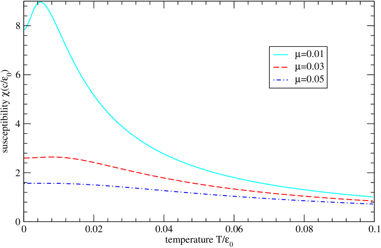
Figure 1: Susceptibility vs temperature for different values of chemical potentials $\mu=0.01,0.03,0.05$ and $h=0.001$. At $T=0$, the susceptibility values for different values of chemical potentials are consistent with the field theory prediction $\chi v_{s}=\theta/\pi$. This possibly gives a way to test effective spin velocities of the spin-1/2 ultracold atoms with a repulsive delta-function interaction.

By substitution of the holon velocity $v_{c}$ and spinon velocity $v_{s}$ at $H=0$ (see (150) in Appendix C), the free energy (42) suggests the universal low temperature form of spin-charge separation theory, namely

$$F=E_{0}-\frac{\pi CT^{2}}{6}\left(\frac{1}{v_{s}}+\frac{1}{v_{c}}\right),$$ (49)

where $E_{0}$ denotes the ground state energy density and $C=1$. The above behavior can also be derived for generic $c$ and $H$ (see Appendix C). This expression corresponds to two central charge $C=1$ conformal field theories Affleck1986 . This universal nature of (49) means that the low-lying excitations are decoupled into two massless degrees of freedom which are described by two Gaussian theories. However, if the excitations involve highly excited states, these theories break down. In Fig.  2 we compare the exact thermodynamics with the predictions of conformal field theory and show the breakdown of the two Gaussian theories at higher temperatures.

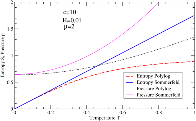
Figure 2: (Color online) Pressure and entropy vs temperature $T$. Solid lines show the pressure (41) and entropy obtained from the free energy (49); dashed lines show pressure and entropy obtained from the polylogarithm function (37) which gives the precise thermodynamics for temperatures below the Fermi temperature $k_{B}T_{F}=E_{F}=\frac{\pi^{2}\hbar^{2}n^{2}}{6m}$ in the strong coupling limit. At low temperatures, they are indeed consistent with the field theory predictions. The deviation of the entropy from the linear temperature dependence marks a breakdown of the two massless field theories.

IV Dressed charge

The excitation spectrum for repulsive spin-1/2 fermions is gapless for any magnetic field strength $H$. As a consequence, the asymptotic behavior of the correlation functions of the model can be described by conformal field theory (CFT) Cardy1986 ; Blote1986 ; Affleck1986 . CFT relates the critical exponents of the correlation functions to the finite-size corrections in the energy spectrum. The basic tool used to determine the critical exponents from the finite-size corrections is the dressed charge matrix. For this model, it is a $2\times 2$ matrix which couples the charge and spin degrees of freedom together and at the same time governs the excitations of charge and spin waves near the Fermi surface.

The dressed charge matrix of this system is explicitly given by

$$\mathbf{Z}=\left(\begin{array}[]{cc}Z_{cc}(k_{0})&Z_{cs}(\lambda_{0})\\ Z_{sc}(k_{0})&Z_{ss}(\lambda_{0})\\ \end{array}\right)$$ (50)

while the integral equations of its elements are given by

$$Z_{cc}(k) = 1+\int_{-\lambda_{0}}^{\lambda_{0}}a_{1}(k-\lambda)Z_{cs}(\lambda)d\lambda$$ (51)

$$Z_{cs}(\lambda) = \int_{-k_{0}}^{k_{0}}a_{1}(\lambda-k)Z_{cc}(k)dk-\int_{-\lambda_{0}}^{\lambda_{0}}a_{2}(\lambda-\mu)Z_{cs}(\mu)d\mu$$ (52)

$$Z_{sc}(k) = \int_{-\lambda_{0}}^{\lambda_{0}}a_{1}(k-\lambda)Z_{ss}(\lambda)d\lambda$$ (53)

$$Z_{ss}(\lambda) = 1+\int_{-k_{0}}^{k_{0}}a_{1}(\lambda-k)Z_{sc}(k)dk-\int_{-\lambda_{0}}^{\lambda_{0}}a_{2}(\lambda-\mu)Z_{ss}(\mu)d\mu.$$ (54)

This set of equations are in turn made up of two coupled sets of equations. Equations (51) and (52) can be treated separately from equations (53) and (54). The following relations are useful for further calculation:

$$\int_{-k_{0}}^{k_{0}}\frac{Z_{sc}(k)}{2\pi}dk =\int_{-\lambda_{0}}^{\lambda_{0}}\frac{Z_{cs}(\lambda)}{2\pi}d\lambda=\int_{-\lambda_{0}}^{\lambda_{0}}\rho_{s}(\lambda)d\lambda=n_{\downarrow}$$ (55)

$$\int_{-k_{0}}^{k_{0}}\frac{Z_{cc}(k)}{2\pi}dk =\int_{-k_{0}}^{k_{0}}\rho_{c}(k)dk=n_{c}$$ (56)

where $n_{\downarrow}$ is the density of down-spin fermions. To derive these relations, we first multiply each set of density equations with the dressed charge equations and integrate them. While making use of the fact that the kernels are symmetric, we then subtract one equation from the other to eliminate the same terms. FIG. 3 shows a depiction of the numerical solutions to Eqs. (51)–(54).

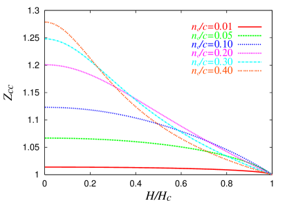
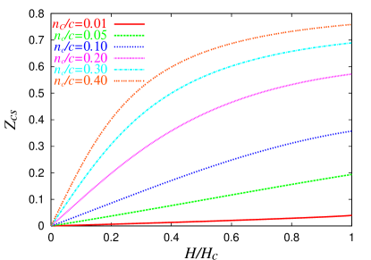
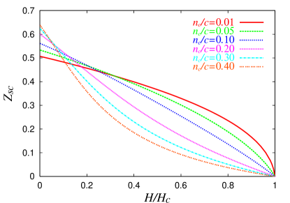
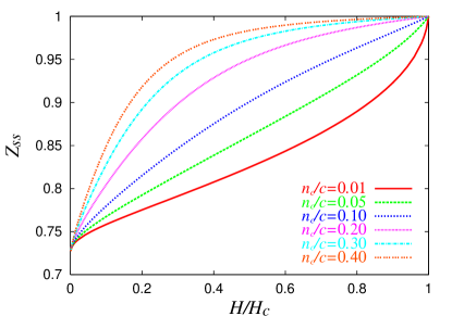
Figure 3: (Color online) This figure shows the dressed charges $Z_{cc}(k_{0})$, $Z_{cs}(\lambda_{0})$, $Z_{sc}(k_{0})$ and $Z_{ss}(\lambda_{0})$ as a function of the external field $H/H_{c}$. The dressed charges are plotted for different values of $n_{c}/c$ which is the inverse of the interaction parameter $\gamma$. These curves are plotted by numerically solving Eqs. (51)–(54).

IV.1 The limit $H\ll 1$

When $H=0$, the ground state of the system is antiferromagnetic. We now solve the dressed charge equations under a small magnetic field by the Wiener-Hopf technique. Considering only terms of up to order $1/c$ in the strong coupling limit, equation (54) can be written as

$$Z_{ss}(\lambda) =1+a_{1}(\lambda)\int_{-k_{0}}^{k_{0}}Z_{sc}(k)dk-\int_{-\lambda_{0}}^{\lambda_{0}}a_{2}(\lambda-\mu)Z_{ss}(\mu)d\mu$$

$$=1+2\pi n_{\downarrow}a_{1}(\lambda)-\int_{-\lambda_{0}}^{\lambda_{0}}a_{2}(\lambda-\mu)Z_{ss}(\mu)d\mu$$ (57)

where the property (55) was used. Applying the Fourier transform, we obtain

$$Z_{ss}(\lambda)=\frac{1}{2}+2\pi n_{\downarrow}s(\lambda)+\int_{|\mu|\geq\lambda_{0}}K(\lambda-\mu)Z_{ss}(\mu)d\mu.$$ (58)

This equation is the same as Eq. (16) other than the driving term, and hence a similar procedure as introduced in Section III is applicable. Introducing the function $y(\lambda)=Z_{ss}(\lambda+\lambda_{0})$ and expanding it as $y(\lambda)=\sum_{n=0}^{\infty}y_{n}(\lambda)$, we obtain the integral equation (see the corresponding equation (28) in Sec. III)

$$y_{n}(\lambda)=g_{n}(\lambda)+\int_{0}^{\infty}K(\lambda-\mu)y_{n}(\mu)d\mu$$ (59)

where $g_{n}(\lambda)$ is given by

$$g_{0}(\lambda)=\frac{1}{2}+2\pi n_{\downarrow}s(\lambda+\lambda_{0}),$$

$$g_{n}(\lambda)=\int_{0}^{\infty}K(\lambda+\mu+2\lambda_{0})y_{n-1}(\mu)d\mu\qquad(n\geq 1).$$ (60)

For $n=0$, setting $a=1/2$ and $b=2\pi n_{\downarrow}$ in Eq. (131), one has

$$\widehat{y}_{0+}(\omega)=G_{+}(\omega)\left[\frac{iG_{-}(-i\epsilon)}{2(\omega+i\epsilon)}+\frac{2\pi in_{\downarrow}G_{-}(-\pi i/c)e^{-\pi\lambda_{0}/c}}{c(\omega+\pi i/c)}\right]+O(H^{2}).$$ (61)

Combining this result with Eq. (121), and finally substituting the relations (124), (116) and (31), one obtains the first order contribution to $Z_{ss}(\lambda_{0})$:

$$y_{0}(0)=\frac{1}{\sqrt{2}}\left(1+\frac{4n_{\downarrow}}{c}\frac{H}{H_{c}}\right)+O(H^{2}).$$ (62)

To obtain the second order correction to $y(0)=Z_{ss}(\lambda_{0})$, we must consider the contribution of $y_{1}(0)$. The Fourier transform of $g_{1}(\lambda)$ is given by

$$\widehat{g}_{1}(\omega)=e^{-2i\lambda_{0}\omega}\widehat{y}_{0+}(-\omega)\widehat{K}(\omega)=e^{-2i\lambda_{0}\omega}\widehat{y}_{0+}(-\omega)\left[1-\frac{1}{G_{+}(\omega)G_{-}(\omega)}\right].$$ (63)

Here we have used the decomposition of the kernel (116). As demonstrated in Appendix. B, let us decompose $\widehat{g}_{1}(\omega)G_{-}(\omega)$ into the two parts $\Phi_{\pm}(\omega)$ which are analytic in the upper and lower half planes, respectively: $\widehat{g}_{1}(\omega)G_{-}(\omega)=\Phi_{+}(\omega)+\Phi_{-}(\omega)$. Now $\Phi_{+}(\omega)$ is given by

$$\Phi_{+}(\omega)=-\frac{1}{2\pi i}\int_{-\infty}^{\infty}\frac{e^{-2i\lambda_{0}x}\widehat{y}_{0+}(-x)}{x-\omega-i\epsilon}\frac{1}{G_{+}(x)}dx$$ (64)

where $\epsilon$ is a small positive constant. Note that the function $G_{+}(x)$ has a branch cut along the negative imaginary axis. Deforming the integration contour to avoid the branch cut, we have

$$\Phi_{+}(\omega) = \frac{1}{2\pi i}\int_{0}^{\infty}\frac{e^{-2\lambda_{0}x}\widehat{y}_{0+}(ix)}{x-i\omega}\left[\frac{1}{G_{+}(-ix-\epsilon)}-\frac{1}{G_{+}(-ix+\epsilon)}\right]dx$$ (65)

$$= \frac{1}{(2\pi)^{\frac{3}{2}}i}\int_{0}^{\infty}\frac{e^{-2\lambda_{0}x}\widehat{y}_{0+}(ix)}{x-i\omega}\left(\frac{cx}{2\pi e}\right)^{\frac{cx}{2\pi}}\Gamma\left(\frac{1}{2}-\frac{cx}{2\pi}\right)(e^{\frac{icx}{2}}-e^{\frac{-icx}{2}})dx$$

$$= \frac{2}{(2\pi)^{\frac{3}{2}}}\int_{0}^{\infty}\frac{e^{-2\lambda_{0}x}\widehat{y}_{0+}(ix)}{x-i\omega}\left(\frac{cx}{2\pi e}\right)^{\frac{cx}{2\pi}}\Gamma\left(\frac{1}{2}-\frac{cx}{2\pi}\right)\sin\left(\frac{cx}{2}\right)dx$$

$$\approx \frac{1}{2\pi}\int_{0}^{\infty}\frac{e^{-2\lambda_{0}x}}{-i\omega}\left(\frac{c}{\sqrt{2}}+O(x)\right)dx$$

$$= \frac{1}{-i\omega}\left(\frac{c}{4\sqrt{2}\pi\lambda_{0}}+O\left(\frac{1}{\lambda_{0}^{2}}\right)\right).$$

Note that, from the third to the fourth step in the above equation, we have used the fact that the integrand rapidly decreases for $x>0$ because $\lambda_{0}\gg 1$, and hence the integral can be approximated by expanding the terms other than $\exp(-2\lambda_{0}x)$ around $x=0$. By a relation similar to Eq. (120), $\widehat{y}_{1+}(\omega)$ is expressed as

$$\widehat{y}_{1+}(\omega)=G_{+}(\omega)\Phi_{+}(\omega)=\frac{G_{+}(\omega)}{-i\omega}\left(\frac{c}{4\sqrt{2}\pi\lambda_{0}}+O\left(\frac{1}{\lambda_{0}^{2}}\right)\right).$$ (66)

Insertion of the relation (121) and Eq. (116) yields

$$y_{1}(0)=\frac{c}{4\sqrt{2}\pi\lambda_{0}}+O\left(\frac{1}{\lambda_{0}^{2}}\right).$$ (67)

Therefore from (62), (67) and (31), we finally obtain the expression

$$Z_{ss}(\lambda_{0})=\frac{1}{\sqrt{2}}\left[1+\frac{4n_{\downarrow}}{c}\left(\frac{H}{H_{c}}\right)+\frac{1}{4\ln(H_{0}/H)}\right]+O\left(\frac{1}{(\ln H_{0}/H)^{2}}\right).$$ (68)

Next we evaluate the dressed charge $Z_{sc}(k_{0})$. The Fourier transforms of (53) and (58) give

$$Z_{sc}(k)=\frac{1}{2}+2\pi n_{\downarrow}K(k)-\int_{|\mu|\geq\lambda_{0}}s(k-\lambda)Z_{ss}(\lambda)d\lambda.$$ (69)

Applying the same procedure as used in the derivation of Eq. (33), we immediately obtain

$$Z_{sc}(k_{0}) =\frac{1}{2}+2\pi n_{\downarrow}K(k_{0})-\frac{2e^{-\frac{\pi}{c}\lambda_{0}}}{c}\widehat{y}_{0+}\left(\frac{\pi i}{c}\right)$$

$$=\frac{1}{2}+\frac{2n_{\downarrow}\ln 2}{c}-\frac{2}{\pi^{2}}\left(\frac{H}{H_{c}}\right)+O\left(\frac{H}{H_{c}\ln(H_{0}/H)}\right)$$ (70)

where we have used the relation (35).

Repeating this whole process to evaluate $Z_{cs}(\lambda_{0})$ and $Z_{cc}(k_{0})$, we find that

$$Z_{cs}(\lambda_{0})=\frac{2\sqrt{2}n_{c}}{c}\left(\frac{H}{H_{c}}\right)+O\left(\frac{H}{H_{c}(\ln(H_{0}/H))^{2}}\right)$$ (71)

and

$$Z_{cc}(k_{0})=1+\frac{2n_{c}\ln 2}{c}-\frac{4n_{c}}{\pi^{2}c}\left(\frac{H}{H_{c}}\right)^{2}+O\left(\frac{H^{2}}{H^{2}_{c}(\ln(H_{0}/H))^{2}}\right).$$ (72)

The down-spin density $n_{\downarrow}$ can be explicitly written in terms of the external magnetic field $H$ by evaluating Eq. (55). Using the property that $Z_{sc}(k)\approx Z_{sc}(k_{0})+O(1/c^{2})$ for $c\gg 1$ and $k_{0}\approx\pi n_{c}/(1+2\ln 2/\gamma)$ (see Eq. (146)), we find that

$$n_{\downarrow}=\frac{n_{c}}{2}\left[1-\frac{4}{\pi^{2}}\left(\frac{H}{H_{c}}\right)\right].$$ (73)

By substituting the expression (73) into Eqs. (68) and (70), the dressed charges in the strong coupling regime $c\gg 1$ and a weak magnetic field $H\ll 1$ are explicitly determined in terms of the fixed particle density $n_{c}$ and the external magnetic field $H$.

IV.2 The limit $H\rightarrow H_{c}$ for $\gamma\gg 1/\sqrt{1-H/H_{c}}$

When $H\geq H_{c}$, the ground state of the system is ferromagnetic. Correspondingly the Fermi point $\lambda_{0}$ becomes zero. Before solving the dressed charged matrix for $H$ approaching the critical field $H_{c}$ from below, we have to know how $\lambda_{0}$ behaves in this vicinity. The spin part of the TBA equation at $T=0$ (i.e., $\phi_{1}^{(0)}(\lambda)$ in Eq. (16) or equivalently the dressed energy $\varepsilon_{s}(\lambda)$ in Eq. (106)) is approximately

$$\varepsilon_{s}(\lambda) =H+\int_{-k_{0}}^{k_{0}}a_{1}(\lambda-k)\varepsilon_{c}(k)dk-\int_{-\lambda_{0}}^{\lambda_{0}}a_{2}(\lambda-\mu)\varepsilon_{s}(\mu)d\mu$$

$$\approx H-2\pi P_{0}a_{1}(\lambda)-2\lambda_{0}a_{2}(\lambda)\varepsilon_{s}(0)$$ (74)

which is derived by approximating the first integral as in (12) and expanding the second integral around $\lambda_{0}\approx 0$. Let us assume $\gamma\gg 1/\sqrt{1-H/H_{c}}\gg 1$. In this region, one sees from Eq. (111) that Eq. (74) further reduces to

$$\varepsilon_{s}(\lambda)=H-\frac{H_{c}}{1+4\lambda^{2}/c^{2}}-\frac{2\lambda_{0}}{\pi c}\frac{\varepsilon_{s}(0)}{1+\lambda^{2}/c^{2}}.$$ (75)

With this result, we can explicitly find $\varepsilon_{s}(0)$ to be

$$\varepsilon_{s}(0)=-\frac{H_{c}-H}{1+2\lambda_{0}/\pi c}.$$ (76)

The last step to derive an explicit expression for $\lambda_{0}$ is to use the condition $\varepsilon_{s}(\pm\lambda_{0})=0$. This gives

$$H-\frac{H_{c}}{1+4\lambda_{0}^{2}/c^{2}}+\frac{2\lambda_{0}}{\pi c}\frac{H_{c}-H}{(1+\lambda_{0}^{2}/c^{2})(1+2\lambda_{0}/\pi c)}=0.$$ (77)

Multiplying the equation with each denominator and then ignoring the terms of order $O(\lambda_{0}^{3}/c^{3})$ or higher yields the equation

$$H-H_{c}+\frac{5\lambda_{0}^{2}}{c^{2}}H-\frac{\lambda_{0}^{2}}{c^{2}}H_{c}=0.$$ (78)

After rearranging the terms and using the fact that $H\rightarrow H_{c}$, we arrive at the result

$$\lambda_{0}\approx\frac{c}{2}\sqrt{1-\frac{H}{H_{c}}}$$ (79)

which is also similar to the result obtained for the 1D Hubbard model Frahm1991 and the XXZ Heisenberg chain Bogoliubov1986 .

With this expression, we can evaluate the dressed charge matrix explicitly in terms of $H$. For $Z_{cs}(\lambda_{0})$, from (52)

$$Z_{cs}(\lambda)\approx 2\pi a_{1}(\lambda)n_{c}-2\lambda_{0}a_{2}(\lambda)Z_{cs}(0).$$ (80)

Here an approximation similar to the above and the property (56) have been used. Solving for $Z_{cs}(0)$ and neglecting terms of order $O(1/c^{2})$, we have $Z_{cs}(0)\approx 4/\gamma$. Substituting this together with (79) implies that

$$Z_{cs}(\lambda_{0})\approx\frac{4}{\gamma}\left(1-\frac{1}{\pi}\sqrt{1-\frac{H}{H_{c}}}\right).$$ (81)

$Z_{cc}(k_{0})$ is easily obtained by substituting the above results into the approximation form $Z_{cc}(k_{0})\approx 1+2\lambda_{0}a_{1}(k_{0})Z_{cs}(0)$ of Eq. (51). The result reads

$$Z_{cc}(k_{0})\approx 1+\frac{8}{\pi\gamma}\sqrt{1-\frac{H}{H_{c}}}.$$ (82)

The remaining dressed charges $Z_{ss}(\lambda_{0})$ and $Z_{sc}(k_{0})$ are also evaluated by similar calculations. For $Z_{ss}(\lambda_{0})$, Eq. (54) becomes $Z_{ss}(\lambda)=1+2\pi n_{\downarrow}a_{1}(\lambda)-2\lambda_{0}a_{2}(\lambda)Z_{ss}(0)$, and hence $Z_{ss}(\lambda_{0})=1+4n_{\downarrow}/c-2\lambda_{0}/(\pi c)$. The density of down-spin fermions $n_{\downarrow}$ is evaluated by applying the same method as in the above to Eq. (103), with result

$$n_{\downarrow}=\int_{-\lambda_{0}}^{\lambda_{0}}\rho_{s}(\lambda)d\lambda\approx 2\lambda_{0}\rho_{s}(0)\approx\frac{2n_{c}}{\pi}\sqrt{1-\frac{H}{H_{c}}}.$$ (83)

This in turn gives

$$Z_{ss}(\lambda_{0})\approx 1-\frac{1}{\pi}\sqrt{1-\frac{H}{H_{c}}}+\frac{8}{\pi\gamma}\sqrt{1-\frac{H}{H_{c}}}.$$ (84)

Likewise,

$$Z_{sc}(k_{0})\approx\frac{2}{\pi}\sqrt{1-\frac{H}{H_{c}}}.$$ (85)

In FIG. 4, we compare the numerical solutions to the leading order solutions for the dressed charges in both limits $H\ll 1$ and $H\rightarrow H_{c}$. It shows good agreement between our leading order solutions and the numerical solutions at points not far from $H=0$ and $H=H_{c}$.

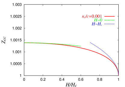
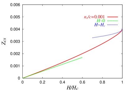
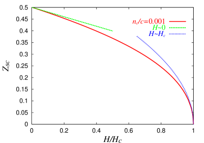
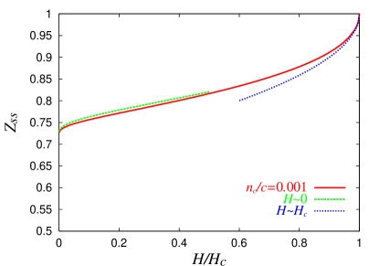
Figure 4: (Color online) This figure shows a comparison between the numerical solutions (solid lines) and the leading order corrections to the dressed charges $Z_{cc}(k_{0})$, $Z_{cs}(\lambda_{0})$, $Z_{sc}(k_{0})$ and $Z_{ss}(\lambda_{0})$ in the limits $H\ll 1$ and $H\rightarrow H_{c}$ for $n_{c}/c=0.001$.

V Correlation functions

We turn now to the calculation of the long distance asymptotics of various correlation functions and scaling dimensions which have been obtained for the 1D Hubbard model in terms of the dressed charge formalism book3 ; Frahm1990 ; Frahm1991 . Our results extend these results into the strong but finite coupling regime for the spin-1/2 repulsive fermion model.

The spin-1/2 repulsive fermion model is gapless and thus critical at zero temperature. At $T=0$, the correlation functions decay as some power of distance governed by the critical exponent which we shall denote conventionally by $\theta$. For $T>0$ the decay is exponential. It was shown that conformal invariance leads to universality classes of critical theories that are related to the central charge $C$ related to the underlying Virasoro algebra Belavin1984 . The critical behavior of the model under consideration is described by the direct product of two Virasoro algebras, one characterizing the spin degree and the other characterizing the charge degree. Both Virasoro algebras have central charge $C=1$.

The general two-point correlation function for primary fields $\varphi$ with conformal dimensions $\Delta^{\pm}_{c,s}$ at $T=0$ and $T>0$ are given by

$$\langle\varphi(x,t)\varphi(0,0)\rangle=\frac{\exp(-2iD_{c}(k_{F\uparrow}+k_{F\downarrow})x)\exp(-2iD_{s}k_{F\downarrow}x)}{(x-iv_{c}t)^{2\Delta^{+}_{c}}(x+iv_{c}t)^{2\Delta^{-}_{c}}(x-iv_{s}t)^{2\Delta^{+}_{s}}(x+iv_{s}t)^{2\Delta^{-}_{s}}}$$ (86)

and

$$\langle\varphi(x,t)\varphi(0,0)\rangle_{T}$$ (87)

$$=\exp(-2iD_{c}(k_{F\uparrow}+k_{F\downarrow})x)\exp(-2iD_{s}k_{F\downarrow}x)$$

$$\times\left(\frac{\pi T}{v_{c}\sinh(\pi T(x-iv_{c}t)/v_{c})}\right)^{2\Delta_{c}^{+}}\left(\frac{\pi T}{v_{c}\sinh(\pi T(x+iv_{c}t)/v_{c})}\right)^{2\Delta_{c}^{-}}$$

$$\times\left(\frac{\pi T}{v_{s}\sinh(\pi T(x-iv_{s}t)/v_{s})}\right)^{2\Delta_{s}^{+}}\left(\frac{\pi T}{v_{s}\sinh(\pi T(x+iv_{s}t)/v_{s})}\right)^{2\Delta_{s}^{-}}$$

where $k_{F\downarrow,\uparrow}$ are the Fermi momenta, $0<x\leq L$ and $-\infty<t<\infty$ is Euclidean time. The conformal dimensions of the fields can be written in terms of the elements of the dressed charge matrix as

$$2\Delta_{c}^{\pm}(\Delta N_{c,s},N^{\pm}_{c,s},D_{c,s})=\left(Z_{cc}D_{c}+Z_{sc}D_{s}\pm\frac{Z_{ss}\Delta N_{c}-Z_{cs}\Delta N_{s}}{2\det Z}\right)^{2}+2N_{c}^{\pm}$$ (88)

and

$$2\Delta_{s}^{\pm}(\Delta N_{c,s},N^{\pm}_{c,s},D_{c,s})=\left(Z_{cs}D_{c}+Z_{ss}D_{s}\pm\frac{Z_{cc}\Delta N_{s}-Z_{sc}\Delta N_{c}}{2\det Z}\right)^{2}+2N_{s}^{\pm}.$$ (89)

The non-negative integers $\Delta N_{\alpha}$, $N_{\alpha}^{\pm}$ and the parameter $D_{\alpha}$ where $\alpha=c,s$ represent the three types of low-lying excitations. Here $\Delta N_{\alpha}$ denotes the change in the number of down-spin fermions. $N_{\alpha}^{\pm}$ characterizes particle-hole excitations where $N_{\alpha}^{+}$ ($N_{\alpha}^{-}$) is the number of occupancies that a particle at the right (left) Fermi level jumps to. $N_{\alpha}^{\pm}$ also enumerates the descendent fields for the primary fields $\varphi$. And lastly, $D_{\alpha}$ represents fermions that are backscattered from one Fermi point to the other. They are restricted by the condition

$$D_{c}\equiv\frac{\Delta N_{s}+\Delta N_{s}}{2}\quad(\mathrm{mod}1),\qquad D_{s}\equiv\frac{\Delta N_{c}}{2}\quad(\mathrm{mod}1).$$ (90)

We want to find the asymptotic behavior of the general two-point correlation functions for the operators $O(x,t)$, namely $\langle O(x,t)O^{\dagger}(0,0)\rangle$. The operators can be written as a linear combination of primary fields with conformal dimensions $\Delta^{\pm}_{c,s}$ and their descendent fields. Noting that the correlation functions for fields with different conformal dimensions are zero, we can express the correlation functions at $T=0$ and $T>0$ respectively as

$$\langle O(x,t)O^{\dagger}(0,0)\rangle=\sum_{\mathbf{n}}A(\Delta N_{c,s},N^{\pm}_{c,s},D_{c,s})\frac{\exp(-2iD_{c}(k_{F\uparrow}+k_{F\downarrow})x)\exp(-2iD_{s}k_{F\downarrow}x)}{(x-iv_{c}t)^{2\Delta^{+}_{c}}(x+iv_{c}t)^{2\Delta^{-}_{c}}(x-iv_{s}t)^{2\Delta^{+}_{s}}(x+iv_{s}t)^{2\Delta^{-}_{s}}}$$ (91)

and

$$\langle O(x,t)O^{\dagger}(0,0)\rangle_{T}$$ (92)

$$=\sum_{\mathbf{n}}A(\Delta N_{c,s},N^{\pm}_{c,s},D_{c,s})\exp(-2iD_{c}(k_{F\uparrow}+k_{F\downarrow})x)\exp(-2iD_{s}k_{F\downarrow}x)$$

$$\times\left(\frac{\pi T}{v_{c}\sinh(\pi T(x-iv_{c}t)/v_{c})}\right)^{2\Delta_{c}^{+}}\left(\frac{\pi T}{v_{c}\sinh(\pi T(x+iv_{c}t)/v_{c})}\right)^{2\Delta_{c}^{-}}$$

$$\times\left(\frac{\pi T}{v_{s}\sinh(\pi T(x-iv_{s}t)/v_{s})}\right)^{2\Delta_{s}^{+}}\left(\frac{\pi T}{v_{s}\sinh(\pi T(x+iv_{s}t)/v_{s})}\right)^{2\Delta_{s}^{-}}$$

where $\mathbf{n}$ denotes the set of quantum numbers

$$\mathbf{n}=(\Delta N_{c,s},N^{\pm}_{c,s},D_{c,s})$$ (93)

which are determined by the condition given in (90) and the selection rules for the form factors while performing a spectral decomposition of the correlation functions Cardy1986 .

Let us consider the correlation functions of operators which are written in terms of the field operators $\psi_{\sigma}(x,t)$ where $\sigma=\uparrow,\downarrow$. They obey the canonical commutation relations

$$\{\psi_{\sigma}(x,t),\psi_{\sigma^{\prime}}^{\dagger}(x,t^{\prime})\} = \delta_{\sigma\sigma^{\prime}}\delta(x-x^{\prime})$$

$$\{\psi_{\sigma}(x,t),\psi_{\sigma}(x,t^{\prime})\} = \{\psi_{\sigma}^{\dagger}(x,t),\psi_{\sigma}^{\dagger}(x,t^{\prime})\}=0.$$ (94)

Here we consider the following correlation functions:

(i) One particle Green’s function:

$$G_{\sigma}(x,t)=\langle\psi_{\sigma}(x,t)\psi_{\sigma}^{\dagger}(0,0)\rangle.$$ (95)

(ii) Charge density correlation function:

$$G_{nn}(x,t)=\langle n(x,t)n(0,0)\rangle$$ (96)

where

$$n(x,t)=n_{\uparrow}(x,t)+n_{\downarrow}(x,t),\qquad n_{\sigma}(x,t)=\psi_{\sigma}^{\dagger}(x,t)\psi_{\sigma}(x,t).$$ (97)

(iii) Longitudinal spin-spin correlation function:

$$G^{z}(x,t)=\langle S^{z}(x,t)S^{z}(0,0)\rangle$$ (98)

where

$$S^{z}(x,t)=\frac{1}{2}(n_{\uparrow}(x,t)-n_{\downarrow}(x,t)).$$ (99)

(iv) Transverse spin-spin correlation function:

$$G^{\perp}(x,t)=\langle S^{+}(x,t)S^{-}(0,0)\rangle$$ (100)

where

$$S^{+}(x,t)=\psi_{\uparrow}^{\dagger}(x,t)\psi_{\downarrow}(x,t),\qquad S^{-}(x,t)=\psi_{\downarrow}^{\dagger}(x,t)\psi_{\uparrow}(x,t).$$ (101)

(v) Pair correlation function:

$$G_{p}(x,t)=\langle\psi_{\downarrow}(x,t)\psi_{\uparrow}(x,t)\psi_{\uparrow}^{\dagger}(0,0)\psi_{\downarrow}^{\dagger}(0,0)\rangle.$$ (102)

For each of the correlation functions considered above, the values of $\mathbf{n}$ are given by

$$G_{\uparrow}(x,t) : (\Delta N_{c}=1,\Delta N_{s}=0,D_{c}\in\mathbb{Z}+1/2,D_{s}\in\mathbb{Z}+1/2)$$

$$G_{\downarrow}(x,t) : (\Delta N_{c}=1,\Delta N_{s}=1,D_{c}\in\mathbb{Z},D_{s}\in\mathbb{Z}+1/2)$$

$$G_{nn}(x,t) : (\Delta N_{c}=0,\Delta N_{s}=0,D_{c}\in\mathbb{Z},D_{s}\in\mathbb{Z})$$

$$G^{z}(x,t) : (\Delta N_{c}=0,\Delta N_{s}=0,D_{c}\in\mathbb{Z},D_{s}\in\mathbb{Z})$$

$$G^{\perp}(x,t) : (\Delta N_{c}=0,\Delta N_{s}=1,D_{c}\in\mathbb{Z}+1/2,D_{s}\in\mathbb{Z})$$

$$G_{p}(x,t) : (\Delta N_{c}=2,\Delta N_{s}=1,D_{c}\in\mathbb{Z}+1/2,D_{s}\in\mathbb{Z}).$$

with $N^{\pm}_{c,s}\in\mathbb{Z}_{\geq 0}$ for every case. The explicit results for these correlation functions for $H\ll 1$ and $H\to H_{c}$ are given in Appendices D and E, which include the order of $1/\gamma$ corrections in the critical exponents.

VI Conclusion

We have derived the low temperature thermodynamics and long distance asymptotics of correlation functions for the spin-1/2 repulsive delta-function interacting Fermi gas with an external field by means of the thermodynamic Bethe ansatz method and dressed charge formalism. With the help of Wiener-Hopf techniques we have calculated the low temperature free energy and thermodynamics and found that the low energy physics can be described by a spin-charge separated theory of a Tomonaga-Luttinger liquid and an antiferromagnetic spin Heisenberg chain. The dressed charge equations have been solved analytically for a small external field $H\to 0$ and a large external field $H\to H_{c}$ using the Wiener-Hopf method. We have also calculated the conformal dimensions for many correlation functions including the one particle Green’s function, the charge density correlation function and pairing correlation, as given in Section V.

In particular, the explicit form of the critical exponents which we have obtained in terms of the external magnetic field and the interaction strength up to $1/c$ corrections extends the known results obtained for the 1D Hubbard model in the infinite coupling limit book3 ; Frahm1990 . They provide insight into understanding the critical behaviour of interacting fermions in 1D. The result for the free energy at low temperature shows a universal signature of Tomonaga-Luttinger liquids where the leading low temperature contributions are solely dependent on the spin and charge velocities. It is to be expected that this universal nature can be tested via the finite temperature density profiles of the repulsive Fermi gas in an harmonic trap. This opens a way to experimentally observe how the low temperature thermodynamics of a 1D many-body system naturally separates into two free Gaussian field theories.

We have also presented results for the low temperature thermodynamics which extend beyond the range covered by spin-charge separation theory. As effective as it is, the Wiener-Hopf method does not allow the full derivation of the equation of state for temperatures beyond the Tomonaga-Luttinger liquid regime. This is because the Tomonaga-Luttinger low temperature physics does not contain enough information on thermal fluctuations necessary to describe the quantum critical regime. This restricts access to quantum criticality in the whole physical regime. However, as we have demonstrated, the polylog formalism is suitable for the study of low temperature and strong coupling in the $\mu-H$ phase plane for weak magnetic field. The pressure we obtained captures the essential spin density and charge density fluctuations at criticality and may possibly be used to test the spin-charge separation theory in experiment with ultracold atomic fermions. This points to the further study of quantum criticality in 1D interacting Fermi gases with repulsive interaction, as has been done recently for attractive interaction and for the Lieb-Liniger Bose gas GHo ; GBat .

This work has been supported by the Australian Research Council. The authors thank Professor Tin-Lun Ho and Professor Rafael I. Nepomechie for helpful discussions.

Appendix A The ground state properties

Here we briefly describe the ground state properties of spin-1/2 fermions with repulsive interaction. The full spectrum of the Hamiltonian can be obtained by the BA method Yang ; Gaudin . In the thermodynamic limit, the ground state properties are characterized by two Fermi seas made up of charges and (down) spins. The distribution functions $\rho_{c}(k)$ of charges with holon momentum $k$, and $\rho_{s}(k)$ of down spins with spinon rapidity $\lambda$ are written as integral equations,

$$\rho_{c}(k) =\frac{1}{2\pi}+\int_{-\lambda_{0}}^{\lambda_{0}}a_{1}(k-\lambda)\rho_{s}(\lambda)d\lambda$$

$$\rho_{s}(\lambda) =\int_{-k_{0}}^{k_{0}}a_{1}(\lambda-k)\rho_{c}(k)dk-\int_{-\lambda_{0}}^{\lambda_{0}}a_{2}(\lambda-\mu)\rho_{s}(\mu)d\mu$$ (103)

where the function $a_{n}(x)$ is given by (8) and $\pm k_{0}$ and $\pm\lambda_{0}$ correspond to the Fermi points. The density of the fermions $n_{c}=n_{\uparrow}+n_{\downarrow}$ ($n_{\sigma}$ denotes the density of spin-$\sigma$ fermions) and the density of the down-spin fermions $n_{\downarrow}$ are respectively given by

$$\int_{-k_{0}}^{k_{0}}\rho_{c}(k)dk=n_{c},\qquad\int_{-\lambda_{0}}^{\lambda_{0}}\rho_{s}(\lambda)d\lambda=n_{\downarrow}.$$ (104)

The ground state energy per unit length (denoted by $E_{0}$) is

$$E_{0}-\mu n_{c}=-P_{0}=\int_{-k_{0}}^{k_{0}}(k^{2}-\mu-H/2)\rho_{c}(k)dk+H\int_{-\lambda_{0}}^{\lambda_{0}}\rho_{s}(\lambda)d\lambda$$ (105)

where $P_{0}$ is the pressure at zero-temperature (see (9) for finite temperature). The ground state properties are also described in terms of the charge dressed energy $\varepsilon_{c}(k)$ and the spin dressed energy $\varepsilon_{s}(\lambda)$ as

$$\varepsilon_{c}(k) =k^{2}-\mu-H/2+\int_{-\lambda_{0}}^{\lambda_{0}}a_{1}(k-\lambda)\varepsilon_{s}(\lambda)d\lambda$$

$$\varepsilon_{s}(\lambda) =H+\int_{-k_{0}}^{k_{0}}a_{1}(\lambda-k)\varepsilon_{c}(k)dk-\int_{-\lambda_{0}}^{\lambda_{0}}a_{2}(\lambda-\mu)\varepsilon_{s}(\mu)d\mu.$$ (106)

The above dressed energies define the energy bands. The ground state corresponds to the fillings of $\varepsilon_{c}(k)\leq 0$ and $\varepsilon_{s}(\lambda)\leq 0$. Thus the Fermi points $\pm k_{0}$ and $\pm\lambda_{0}$ are given by the conditions

$$\varepsilon_{c}(\pm k_{0})=0,\qquad\varepsilon_{s}(\pm\lambda_{0})=0.$$ (107)

Using the above dressed energies, $E_{0}$ is written as

$$E_{0}-\mu n_{c}=-P_{0}=\frac{1}{2\pi}\int_{-k_{0}}^{k_{0}}\varepsilon_{c}(k)dk.$$ (108)

One can immediately realize that the dressed energies $\varepsilon_{c}(k)$ and $\varepsilon_{s}(\lambda)$ respectively correspond to $\varepsilon(k)$ and $\phi_{1}(\lambda)$ in the TBA equations (2) and (3) in the limit $T\to 0$.

Let us evaluate the value of the critical field $H=H_{c}$. At this point, the density of down-spin electrons is zero ($n_{\downarrow}=0$) i.e., $\lambda_{0}=0$. Therefore the expressions (103) and (106) are significantly simplified. Inserting $\rho_{c}(k)=1/(2\pi)$ into (104), one has $k_{0}=\pi n_{c}$. The Fermi point $k_{0}$ is also calculated by $\varepsilon_{c}(k)=k^{2}-\mu-H_{c}/2$ (106) and the condition (107), i.e. $k_{0}^{2}=\mu+H_{c}/2$. Substituting these expressions into $\varepsilon_{s}(\lambda)$ and using the condition (107), one finally arrives at

$$H_{c}=\left(\frac{c^{2}}{2\pi}+2\pi n_{c}^{2}\right)\tan^{-1}\left(\frac{2\pi n_{c}}{c}\right)-cn_{c}.$$ (109)

The pressure $P_{0}$ at $H=H_{c}$ is

$$P_{0}=\frac{2}{3}\pi^{2}n_{c}^{3}.$$ (110)

In the strong coupling limit $c\gg 1$, $H_{c}$ and $P_{0}$ are given by

$$H_{c}\approx\frac{8\pi^{2}n_{c}^{2}}{3\gamma}\left(1-\frac{4\pi^{2}}{5\gamma^{2}}\right),\qquad P_{0}\approx\frac{n_{c}\gamma H_{c}}{4}\left(1+\frac{4\pi^{2}}{5\gamma^{2}}\right).$$ (111)

Appendix B The Wiener-Hopf method

In this appendix, we briefly review how to solve the integral equations appearing in the main text (see Eq. (28) for instance) by using the Wiener-Hopf method.

Consider a Wiener-Hopf integral equation

$$y(\lambda)=g(\lambda)+\int_{0}^{\infty}K(\lambda-\mu)y(\mu)d\mu$$ (112)

which determines an unknown function $y(\lambda)$ where $K(\lambda)$ is defined by Eq. (8), and the driving term $g(\lambda)$ defined on the entire real axis is assumed to be a known function. By Fourier transforming Eq. (112), we obtain

$$\widehat{y}_{+}(\omega)=\left(1-\widehat{K}(\omega)\right)^{-1}\left(\widehat{g}(\omega)-\widehat{y}_{-}(\omega)\right)$$ (113)

where the functions $\widehat{y}_{\pm}(\omega)$ are defined by

$$\widehat{y}_{\pm}(\omega)=\int_{-\infty}^{\infty}\theta(\pm\lambda)y(\lambda)e^{i\lambda\omega}d\lambda$$ (114)

with $\theta(\lambda)$ representing the Heaviside step function. The function $\widehat{K}(\omega)$ can be explicitly written as

$$\widehat{K}(\omega)=\frac{e^{-c|\omega|/2}}{2\cosh(c|\omega|/2)}.$$ (115)

Eqs. (114) denote a decomposition of $\widehat{y}(\omega)$ into the sum of functions analytic on the upper and lower half-planes, respectively, with $\widehat{y}(\omega)=\widehat{y}_{+}(\omega)+\widehat{y}_{-}(\omega)$. Hereafter we assume that $\widehat{y}_{\pm}(\infty)=\widehat{g}(\infty)=0$.

To solve the equation, we factorize the term $1-\widehat{K}(\omega)$ as

$$\left(1-\widehat{K}(\omega)\right)^{-1}=G_{+}(\omega)G_{-}(\omega),\qquad\lim_{\omega\to\infty}G_{\pm}(\omega)=1$$ (116)

where $G_{+}(\omega)$ ($G_{-}(\omega)$) is a function which is analytic and nonzero in the upper (lower) half-plane. Since $\widehat{K}(\omega)=\widehat{K}(-\omega)$, one finds $G_{+}(\omega)/G_{-}(-\omega)=G_{+}(-\omega)/G_{-}(\omega)$. Therefore $G_{+}(\omega)/G_{-}(-\omega)$ is a bounded entire function. Liouville’s theorem and the asymptotics of $G_{\pm}(\omega)$ yield

$$G_{+}(\omega)=G_{-}(-\omega).$$ (117)

Using the factorization equation (116), Eq. (113) becomes

$$\frac{\widehat{y}_{+}(\omega)}{G_{+}(\omega)}-\Phi_{+}(\omega)=\Phi_{-}(\omega)-G_{-}(\omega)\widehat{y}_{-}(\omega)$$ (118)

where $\Phi_{\pm}(\omega)$ are functions assumed to be analytic and bounded in the upper and lower half planes, respectively,

$$G_{-}(\omega)\widehat{g}(\omega)=\Phi_{+}(\omega)+\Phi_{-}(\omega).$$ (119)

From Eq. (118), the function $\widehat{y}_{+}(\omega)/G_{+}(\omega)-\Phi_{+}(\omega)$ is a bounded entire function, and hence is a constant according to Liouville’s theorem. Considering the asymptotics, we obtain

$$\widehat{y}_{+}(\omega)=G_{+}(\omega)\left(\Phi_{+}(\omega)-\Phi_{+}(\infty)\right),\qquad\widehat{y}_{-}(\omega)=\frac{1}{G_{-}(\omega)}\left(\Phi_{-}(\omega)-\Phi_{-}(\infty)\right).$$ (120)

A formula useful for practical calculations is

$$y(0)=\frac{1}{2\pi}\int_{-\infty}^{\infty}\widehat{y}(\omega)e^{-i\omega\epsilon}d\omega=\frac{1}{2\pi}\int_{C^{-}}\widehat{y}_{+}(\omega)e^{-i\omega\epsilon}d\omega=-i\lim_{\omega\to\infty}\omega\widehat{y}_{+}(\omega)$$ (121)

where $C^{-}$ is a semi-circular path on the lower half-plane. We have used the fact that the sum of residues in the lower half-plane is equal to the residue at the point at infinity.

Next we will determine the explicit forms of $\widehat{y}_{\pm}(\omega)$ by adopting some specific driving terms $g(\lambda)$ appearing in the main text. First let us determine the factors $G_{\pm}(\omega)$. Using the explicit form of $\widehat{K}(\omega)$ in (8), we have

$$2e^{-c|\omega|/2}\cosh(c\omega/2)=G_{+}(\omega)G_{-}(\omega).$$ (122)

The well-known relation $\Gamma(1/2+x)\Gamma(1/2-x)=\pi/\cos\pi x$ Gradshteyn together with the asymptotic form $\Gamma(x)\approx\sqrt{2\pi}x^{x-\frac{1}{2}}e^{-x}$ for $|x|\gg 1$ and the condition for $G_{\pm}(\omega)$ in Eq. (116) yield

$$G_{+}(\omega)=G_{-}(-\omega)=\frac{\sqrt{2\pi}}{\Gamma(\frac{1}{2}-\frac{ic\omega}{2\pi})}\left(\frac{2\pi e}{\epsilon-icw}\right)^{\frac{ic\omega}{2\pi}}$$ (123)

where $\epsilon\to 0+$. Useful special values are

$$G_{\pm}(0)=\sqrt{2},\qquad G_{+}\left(\frac{\pi i}{c}\right)=G_{-}\left(-\frac{\pi i}{c}\right)=\sqrt{\frac{\pi}{e}}.$$ (124)

B.1 The case $g(\lambda)=a+bs(\lambda+\lambda_{0})$

Set the driving term to be $g(\lambda)=a+bs(\lambda+\lambda_{0})$, where $a,b\in\mathbb{C}$. Taking the Fourier transform yields

$$\widehat{g}(\omega)=2\pi a\delta(\omega)+\frac{be^{-i\lambda_{0}\omega}}{2\cosh(c\omega/2)}.$$ (125)

Let us decompose the function as in (119). The first term can be easily decomposed by using

$$\delta(\omega)=\frac{1}{2\pi i}\left(\frac{1}{\omega-i\epsilon}-\frac{1}{\omega+i\epsilon}\right)\qquad(\epsilon\to+0).$$ (126)

On the other hand, the second term in (125) is a meromorphic function whose poles are simple poles (denoted by $\omega_{n}$) located at

$$\omega_{n}=\frac{\pi i}{c}(2n+1)\qquad(n\in\mathbb{Z}).$$ (127)

Thus the decomposition of the function $1/\cosh(c\omega/2)$ reads

$$\frac{1}{\cosh(c\omega/2)} = Q_{+}(\omega)+Q_{-}(\omega),$$

$$Q_{+}(\omega) = \frac{2i}{c}\sum_{n=0}^{\infty}\frac{(-1)^{n}}{\omega+\omega_{n}},$$

$$Q_{-}(\omega) = \frac{1}{\cosh(c\omega/2)}-\frac{2i}{c}\sum_{n=0}^{\infty}\frac{(-1)^{n}}{\omega+\omega_{n}}.$$ (128)

Using this, we can express the function $f_{-}(\omega)/\cosh(c\omega/2)$, where $f_{-}(\omega)$ is any function which is analytic and bounded in the lower half-plane, as

$$\frac{f_{-}(\omega)}{\cosh(c\omega/2)} = \chi_{+}(\omega)+\chi_{-}(\omega),$$

$$\chi_{+}(\omega) = \frac{2i}{c}\sum_{n=0}^{\infty}\frac{(-1)^{n}f_{-}(-\omega_{n})}{\omega+\omega_{n}},$$

$$\chi_{-}(\omega) = \frac{f_{-}(\omega)}{\cosh(c\omega/2)}-\frac{2i}{c}\sum_{n=0}^{\infty}\frac{(-1)^{n}(f_{-}(-\omega_{n}))}{\omega+\omega_{n}}.$$ (129)

Applying the formula (129) to (125) and (119), we obtain, for instance,

$$\Phi_{+}(\omega)=a\frac{iG_{-}(-i\epsilon)}{\omega+i\epsilon}+b\frac{i}{c}\sum_{n=0}^{\infty}\frac{(-1)^{n}G_{-}(-\omega_{n})e^{i\lambda_{0}\omega_{n}}}{\omega+\omega_{n}}.$$ (130)

Substitution of the above equation and (127) into (120) then yields

$$\widehat{y}_{+}(\omega)=G_{+}(\omega)\left[a\frac{iG_{-}(-i\epsilon)}{\omega+i\epsilon}+b\frac{i}{c}\frac{G_{-}(-\pi i/c)e^{-\pi\lambda_{0}/c}}{\omega+\pi i/c}+\cdots\right].$$ (131)

B.2 The case $g(\lambda)=aK(\lambda)$

Next we consider the case $g(\lambda)=aK(\lambda)$ ($a\in\mathbb{C}$). Using the factorization equation (116), one finds

$$\widehat{g}(\omega)=a\widehat{K}(\omega)=a\left(1-\frac{1}{G_{+}(\omega)G_{-}(\omega)}\right).$$ (132)

Thus we immediately obtain $\Phi_{\pm}(\omega)$ defined by Eq. (119), namely

$$\Phi_{+}(\omega)=-\frac{a}{G_{+}(\omega)},\qquad\Phi_{-}(\omega)=aG_{-}(\omega).$$ (133)

Then $\widehat{y}_{\pm}(\omega)$ are respectively given by

$$\widehat{y}_{+}(\omega)=a(G_{+}(\omega)-1),\qquad\widehat{y}_{-}(\omega)=a\left(1-\frac{1}{G_{-}(\omega)}\right).$$ (134)

Appendix C Low-temperature behavior for arbitrary $c>0$

In Section III, we derived the explicit low-temperature thermodynamics (see (42) for instance) for the strong coupling regime ($c\gg 1$) in weak magnetic field ($H\ll 1$) via the polylogarithm expression for the pressure (37). Here, using the dressed function formalism, we extract the universal low-temperature thermodynamics (49) for arbitrary repulsive coupling $c>0$ in arbitrary magnetic field $H\leq H_{c}$. As shown in Section III, the low-temperature thermodynamics is characterized by the two integral equations

$$\varepsilon(k) =k^{2}-\mu-\frac{H}{2}-Ta_{1}\ast\ln(1+e^{-\phi_{1}(k)/T})$$

$$\phi_{1}(\lambda) =H-Ta_{1}\ast\ln(1+e^{-\varepsilon(\lambda)/T})+Ta_{2}\ast\ln(1+e^{-\phi_{1}(\lambda)/T}).$$ (135)

In the limit $T\to 0$, the above equations coincide with the dressed energies (106).

In completely the same way as in the derivation for Eqs. (16), (23) and (24) one obtains

$$\varepsilon(k) =\widetilde{\varepsilon}^{(0)}(k)+\int_{-\lambda_{0}}^{\lambda_{0}}a_{1}(k-\lambda)\phi_{1}(\lambda)d\lambda$$

$$\phi_{1}(\lambda) =\widetilde{\phi}_{1}^{(0)}+\int_{-k_{0}}^{k_{0}}a_{1}(\lambda-k)\varepsilon(k)dk-\int_{-\lambda_{0}}^{\lambda_{0}}a_{2}(\lambda-\mu)\phi_{1}(\mu)d\mu$$ (136)

where

$$\widetilde{\varepsilon}^{(0)} =k^{2}-\mu-\frac{H}{2}-\frac{\pi^{2}T^{2}}{6\varepsilon^{\prime}_{s}(\lambda_{0})}\left(a_{1}(k-\lambda_{0})+a_{1}(k+\lambda_{0})\right)$$

$$\widetilde{\phi}_{1}^{(0)} =H-\frac{\pi^{2}T^{2}}{6\varepsilon^{\prime}_{c}(k_{0})}\left(a_{1}(\lambda-k_{0})+a_{1}(\lambda+k_{0})\right)+\frac{\pi^{2}T^{2}}{6\varepsilon^{\prime}_{s}(\lambda_{0})}\left(a_{2}(\lambda-\lambda_{0})+a_{2}(\lambda+\lambda_{0})\right).$$ (137)

In this limit, the free energy (9) is reduced to

$$F=\mu n_{c}-\frac{\pi T^{2}}{6\varepsilon_{c}^{\prime}(k_{0})}+\frac{1}{2\pi}\int_{-k_{0}}^{k_{0}}\varepsilon(k)dk.$$ (138)

Applying the dressed function formalism to (136) and (103), we arrive at

$$\frac{1}{2\pi}\int_{-k_{0}}^{k_{0}}\varepsilon(k)dk =\int_{-k_{0}}^{k_{0}}\widetilde{\varepsilon}^{(0)}\rho_{c}(k)dk+\int_{-\lambda_{0}}^{\lambda_{0}}\widetilde{\phi}_{1}^{(0)}\rho_{s}(\lambda)d\lambda$$

$$=E_{0}-\frac{\pi T^{2}}{6}\left(\frac{2\pi\rho_{c}(k_{0})}{\varepsilon^{\prime}_{c}(k_{0})}+\frac{2\pi\rho_{s}(\lambda_{0})}{\varepsilon^{\prime}_{s}(\lambda_{0})}\right)+\frac{\pi T^{2}}{6\varepsilon_{c}^{\prime}(k_{0})}-\mu n_{c}.$$ (139)

This yields

$$F=E_{0}-\frac{\pi T^{2}}{6}\left(\frac{1}{v_{s}}+\frac{1}{v_{c}}\right)$$ (140)

where $v_{c}$ and $v_{s}$ are, respectively, the holon and spinon excitation velocities

$$v_{c}=\frac{\varepsilon_{c}^{\prime}(k_{0})}{2\pi\rho_{c}(k_{0})},\qquad v_{s}=\frac{\varepsilon_{s}^{\prime}(\lambda_{0})}{2\pi\rho_{s}(\lambda_{0})}.$$ (141)

Before closing this Appendix, we reproduce the low-temperature thermodynamics (42) for $c\gg 1$ and $H=0$. At $H=0$, the Fermi point $\lambda_{0}=\infty$. By Fourier transformation, the density functions $\rho_{c}(k)$ and $\rho_{s}(\lambda)$ defined by Eq. (103) reduce to

$$\rho_{c}(k)=\frac{1}{2\pi}+\int_{-k_{0}}^{k_{0}}a_{1}(k-\lambda)\rho_{s}(\lambda)d\lambda$$

$$\rho_{s}(\lambda)=\int_{-k_{0}}^{k_{0}}s(\lambda-k)\rho_{c}(k)dk.$$ (142)

Up to leading order in $1/c$ the second equation reads

$$\rho_{s}(\lambda)\approx s(\lambda)\int_{-k_{0}}^{k_{0}}\rho_{c}(k)dk=n_{c}s(\lambda).$$ (143)

Substituting this equation into the first equation in Eq. (142) yields

$$\rho_{c}(k)\approx\frac{1}{2\pi}+n_{c}\int_{-\infty}^{\infty}a_{1}(k-\lambda)s(\lambda)d\lambda=\frac{1}{2\pi}+n_{c}K(k)\approx\frac{1}{2\pi}+\frac{\ln 2}{\pi\gamma}$$ (144)

where (35) has been used. The dressed energies can be obtained by just taking the limit $T\to 0$, $H\to 0$ and $\lambda_{0}\to\infty$ in Eqs (36) and (16). Explicitly,

$$\varepsilon_{c}(k)\approx k^{2}-\mu-2\pi P_{0}K(k)\approx k^{2}-\mu-2P_{0}\ln 2/c$$

$$\varepsilon_{s}(\lambda)\approx-2\pi P_{0}s(\lambda).$$ (145)

The pressure $P_{0}$ is determined by solving (108). Combining Eq. (144) with Eq. (104) gives the Fermi point

$$k_{0}\approx\frac{\pi n_{c}}{1+\frac{2\ln 2}{\gamma}}\approx\pi n_{c}\left(1-\frac{2\ln 2}{\gamma}\right).$$ (146)

$k_{0}$ is derived from the condition (107), with result

$$k_{0}^{2}=\mu+\frac{2P_{0}\ln 2}{c}.$$ (147)

Substituting these expressions into (108) and taking terms of order $O(1/c)$, one arrives at

$$P_{0}=-E_{0}+\mu n_{c}=\frac{2n_{c}^{3}\pi^{2}}{3}\left(1-\frac{6\ln 2}{\gamma}\right)$$ (148)

where $\mu$ denotes the zero-temperature chemical potential determined by Eqs. (147) and (146):

$$\mu=\pi^{2}n_{c}^{2}\left(1-\frac{16\ln 2}{3\gamma}\right).$$ (149)

The excitation velocities

$$v_{c}\approx 2\pi n_{c}\left(1-\frac{4\ln 2}{\gamma}\right),\qquad v_{s}\approx\frac{2\pi^{3}n_{c}}{3\gamma}\left(1-\frac{6\ln 2}{\gamma}\right).$$ (150)

are evaluated by substituting all the results into Eq. (141). Thus from Eq. (140), one finds that the low-temperature free energy $F$ agrees with Eq. (42) at $H=0$.

Appendix D Correlation functions for $H\ll 1$

Here we consider the leading terms of the zero temperature correlation functions listed in Section V. The conformal dimensions are

$$2\Delta_{c}^{\pm}(\Delta N_{c,s},N^{\pm}_{c,s},D_{c,s})=$$ (151)

$$\left(D_{c}+\frac{1}{2}D_{s}\pm\frac{1}{2}\Delta N_{c}\right)^{2}-\frac{4}{\pi^{2}}\left(\frac{H}{H_{c}}\right)D_{s}\left(D_{c}+\frac{1}{2}D_{s}\pm\frac{1}{2}\Delta N_{c}\right)$$

$$+\frac{4\ln 2}{\gamma}\left[\left(D_{c}+\frac{1}{2}D_{s}\right)^{2}-\frac{1}{4}(\Delta N_{c})^{2}\right]-\frac{8\ln 2}{\pi^{2}\gamma}\left(\frac{H}{H_{c}}\right)D_{s}\left(D_{c}+\frac{1}{2}D_{s}\mp\frac{1}{2}\Delta N_{c}\right)$$

$$\pm\frac{4}{\gamma}\left(\frac{H}{H_{c}}\right)\left(\frac{\Delta N_{c}}{2}-\Delta N_{s}\right)\left(D_{c}+\frac{1}{2}D_{s}\pm\frac{1}{2}\Delta N_{c}\right)+2N^{\pm}_{c}$$

and

$$2\Delta_{s}^{\pm}(\Delta N_{c,s},N^{\pm}_{c,s},D_{c,s})=$$ (152)

$$\frac{1}{2}\left(\Delta N_{s}-\frac{1}{2}\Delta N_{c}\pm D_{s}\right)^{2}+\frac{2}{\pi^{2}}\left(\frac{H}{H_{c}}\right)\Delta N_{c}\left(\Delta N_{s}-\frac{1}{2}\Delta N_{c}\pm D_{s}\right)$$

$$+\frac{1}{4\ln(H_{0}/H)}\left[D_{s}^{2}-\left(\Delta N_{s}-\frac{1}{2}\Delta N_{c}\right)^{2}\right]\pm\frac{4}{\gamma}\left(\frac{H}{H_{c}}\right)\left(D_{c}+\frac{1}{2}D_{s}\right)\left(\Delta N_{s}-\frac{1}{2}\Delta N_{c}\pm D_{s}\right)$$

$$-\frac{4\ln 2}{\pi^{2}\gamma}\left(\frac{H}{H_{c}}\right)\Delta N_{c}\left(\Delta N_{s}-\frac{1}{2}\Delta N_{c}\pm D_{s}\right)+2N^{\pm}_{s}.$$

(i) The leading orders for the field correlator $G_{\uparrow}(x,t)$ come from the set of quantum numbers $(D_{c},D_{s})=(1/2,-1/2)$ and $(1/2,1/2)$. The conformal dimensions corresponding to these sets of quantum numbers are

$$2\Delta_{c}^{+}=\frac{9}{16}-\frac{3\ln 2}{4\gamma}+\frac{3}{2\pi^{2}}\left(\frac{H}{H_{c}}\right)+\frac{3}{2\gamma}\left(\frac{H}{H_{c}}\right)-\frac{\ln 2}{\pi^{2}\gamma}\left(\frac{H}{H_{c}}\right)$$

$$2\Delta_{c}^{-}=\frac{1}{16}-\frac{3\ln 2}{4\gamma}-\frac{1}{2\pi^{2}}\left(\frac{H}{H_{c}}\right)+\frac{1}{2\gamma}\left(\frac{H}{H_{c}}\right)+\frac{3\ln 2}{\pi^{2}\gamma}\left(\frac{H}{H_{c}}\right)$$

$$2\Delta_{s}^{+}=\frac{1}{2}-\frac{2}{\pi^{2}}\left(\frac{H}{H_{c}}\right)-\frac{1}{\gamma}\left(\frac{H}{H_{c}}\right)+\frac{4\ln 2}{\pi^{2}\gamma}\left(\frac{H}{H_{c}}\right)$$

$$2\Delta_{s}^{-}=0$$ (153)

for $(D_{c},D_{s})=(1/2,-1/2)$ and

$$2\Delta_{c}^{+}=\frac{25}{16}+\frac{5\ln 2}{4\gamma}-\frac{5}{2\pi^{2}}\left(\frac{H}{H_{c}}\right)+\frac{5}{2\gamma}\left(\frac{H}{H_{c}}\right)-\frac{\ln 2}{\pi^{2}\gamma}\left(\frac{H}{H_{c}}\right)$$

$$2\Delta_{c}^{-}=\frac{1}{16}+\frac{5\ln 2}{4\gamma}-\frac{1}{2\pi^{2}}\left(\frac{H}{H_{c}}\right)-\frac{1}{2\gamma}\left(\frac{H}{H_{c}}\right)-\frac{5\ln 2}{\pi^{2}\gamma}\left(\frac{H}{H_{c}}\right)$$

$$2\Delta_{s}^{+}=0$$

$$2\Delta_{s}^{-}=\frac{1}{2}-\frac{2}{\pi^{2}}\left(\frac{H}{H_{c}}\right)+\frac{3}{\gamma}\left(\frac{H}{H_{c}}\right)+\frac{4\ln 2}{\pi^{2}\gamma}\left(\frac{H}{H_{c}}\right)$$ (154)

for $(D_{c},D_{s})=(1/2,1/2)$. Hence we obtain

$$G_{\uparrow}(x,t)\approx\frac{A_{1}\cos(k_{F\uparrow}x)}{|x+iv_{c}t|^{\theta_{c1}}|x+iv_{s}t|^{\theta_{s1}}}+\frac{A_{2}\cos((k_{F\uparrow}+2k_{F\downarrow})x)}{|x+iv_{c}t|^{\theta_{c2}}|x+iv_{s}t|^{\theta_{s2}}}$$ (155)

where the exponents are given by

$$\theta_{c1} = \frac{5}{8}-\frac{3\ln 2}{2\gamma}+\frac{1}{\pi^{2}}\left(\frac{H}{H_{c}}\right)+\frac{2}{\gamma}\left(\frac{H}{H_{c}}\right)+\frac{2\ln 2}{\pi^{2}\gamma}\left(\frac{H}{H_{c}}\right)$$

$$\theta_{c2} = \frac{13}{8}+\frac{5\ln 2}{2\gamma}-\frac{3}{\pi^{2}}\left(\frac{H}{H_{c}}\right)+\frac{2}{\gamma}\left(\frac{H}{H_{c}}\right)-\frac{6\ln 2}{\pi^{2}\gamma}\left(\frac{H}{H_{c}}\right)$$

$$\theta_{s1} = \frac{1}{2}-\frac{2}{\pi^{2}}\left(\frac{H}{H_{c}}\right)-\frac{1}{\gamma}\left(\frac{H}{H_{c}}\right)+\frac{4\ln 2}{\pi^{2}\gamma}\left(\frac{H}{H_{c}}\right)$$

$$\theta_{s2} = \frac{1}{2}-\frac{2}{\pi^{2}}\left(\frac{H}{H_{c}}\right)+\frac{3}{\gamma}\left(\frac{H}{H_{c}}\right)+\frac{4\ln 2}{\pi^{2}\gamma}\left(\frac{H}{H_{c}}\right).$$ (156)

(ii) The leading terms for the field correlator $G_{\downarrow}(x,t)$ come from the set of quantum numbers $(D_{c},D_{s})=(0,1/2)$ and $(1,-1/2)$. The corresponding conformal dimensions are

$$2\Delta_{c}^{+}=\frac{9}{16}-\frac{3\ln 2}{4\gamma}-\frac{3}{2\pi^{2}}\left(\frac{H}{H_{c}}\right)-\frac{3}{2\gamma}\left(\frac{H}{H_{c}}\right)+\frac{\ln 2}{\pi^{2}\gamma}\left(\frac{H}{H_{c}}\right)$$

$$2\Delta_{c}^{-}=\frac{1}{16}-\frac{3\ln 2}{4\gamma}+\frac{1}{2\pi^{2}}\left(\frac{H}{H_{c}}\right)-\frac{1}{2\gamma}\left(\frac{H}{H_{c}}\right)-\frac{3\ln 2}{\pi^{2}\gamma}\left(\frac{H}{H_{c}}\right)$$

$$2\Delta_{s}^{+}=\frac{1}{2}+\frac{2}{\pi^{2}}\left(\frac{H}{H_{c}}\right)+\frac{1}{\gamma}\left(\frac{H}{H_{c}}\right)-\frac{4\ln 2}{\pi^{2}\gamma}\left(\frac{H}{H_{c}}\right)$$

$$2\Delta_{s}^{-}=0$$ (157)

for $(D_{c},D_{s})=(0,1/2)$ and

$$2\Delta_{c}^{+}=\frac{25}{16}+\frac{5\ln 2}{4\gamma}+\frac{5}{2\pi^{2}}\left(\frac{H}{H_{c}}\right)-\frac{5}{2\gamma}\left(\frac{H}{H_{c}}\right)+\frac{\ln 2}{\pi^{2}\gamma}\left(\frac{H}{H_{c}}\right)$$

$$2\Delta_{c}^{-}=\frac{1}{16}+\frac{5\ln 2}{4\gamma}+\frac{1}{2\pi^{2}}\left(\frac{H}{H_{c}}\right)+\frac{1}{2\gamma}\left(\frac{H}{H_{c}}\right)+\frac{5\ln 2}{\pi^{2}\gamma}\left(\frac{H}{H_{c}}\right)$$

$$2\Delta_{s}^{+}=0$$

$$2\Delta_{s}^{-}=\frac{1}{2}+\frac{2}{\pi^{2}}\left(\frac{H}{H_{c}}\right)-\frac{3}{\gamma}\left(\frac{H}{H_{c}}\right)-\frac{4\ln 2}{\pi^{2}\gamma}\left(\frac{H}{H_{c}}\right)$$ (158)

for $(D_{c},D_{s})=(1,-1/2)$. This gives

$$G_{\downarrow}(x,t)\approx\frac{A_{1}\cos(k_{F\downarrow}x)}{|x+iv_{c}t|^{\theta_{c1}}|x+iv_{s}t|^{\theta_{s1}}}+\frac{A_{2}\cos((2k_{F\uparrow}+k_{F\downarrow})x)}{|x+iv_{c}t|^{\theta_{c2}}|x+iv_{s}t|^{\theta_{s2}}}$$ (159)

where

$$\theta_{c1} = \frac{5}{8}-\frac{3\ln 2}{2\gamma}-\frac{1}{\pi^{2}}\left(\frac{H}{H_{c}}\right)-\frac{2}{\gamma}\left(\frac{H}{H_{c}}\right)-\frac{2\ln 2}{\pi^{2}\gamma}\left(\frac{H}{H_{c}}\right)$$

$$\theta_{c2} = \frac{13}{8}+\frac{5\ln 2}{2\gamma}+\frac{3}{\pi^{2}}\left(\frac{H}{H_{c}}\right)-\frac{2}{\gamma}\left(\frac{H}{H_{c}}\right)+\frac{6\ln 2}{\pi^{2}\gamma}\left(\frac{H}{H_{c}}\right)$$

$$\theta_{s1} = \frac{1}{2}+\frac{2}{\pi^{2}}\left(\frac{H}{H_{c}}\right)+\frac{1}{\gamma}\left(\frac{H}{H_{c}}\right)-\frac{4\ln 2}{\pi^{2}\gamma}\left(\frac{H}{H_{c}}\right)$$

$$\theta_{s2} = \frac{1}{2}+\frac{2}{\pi^{2}}\left(\frac{H}{H_{c}}\right)-\frac{3}{\gamma}\left(\frac{H}{H_{c}}\right)-\frac{4\ln 2}{\pi^{2}\gamma}\left(\frac{H}{H_{c}}\right).$$ (160)

(iii) The leading terms for the charge density correlator come from the set of quantum numbers $(D_{c},D_{s})=(0,0)$, $(0,1)$, $(1,0)$ and $(1,-1)$. The corresponding conformal dimensions are

$$2\Delta_{c}^{+}=0,\quad 2\Delta_{s}^{+}=0,$$

$$2\Delta_{c}^{-}=0,\quad 2\Delta_{s}^{-}=0,$$ (161)

for $(D_{c},D_{s})=(0,0)$ and

$$2\Delta_{c}^{+}=\frac{1}{4}+\frac{\ln 2}{\gamma}-\frac{2}{\pi^{2}}\left(\frac{H}{H_{c}}\right)-\frac{4\ln 2}{\pi^{2}\gamma}\left(\frac{H}{H_{c}}\right)$$

$$2\Delta_{c}^{-}=\frac{1}{4}+\frac{\ln 2}{\gamma}-\frac{2}{\pi^{2}}\left(\frac{H}{H_{c}}\right)-\frac{4\ln 2}{\pi^{2}\gamma}\left(\frac{H}{H_{c}}\right)$$

$$2\Delta_{s}^{+}=\frac{1}{2}+\frac{1}{4\ln(H_{0}/H)}+\frac{2}{\gamma}\left(\frac{H}{H_{c}}\right)$$

$$2\Delta_{s}^{-}=\frac{1}{2}+\frac{1}{4\ln(H_{0}/H)}+\frac{2}{\gamma}\left(\frac{H}{H_{c}}\right).$$ (162)

for $(D_{c},D_{s})=(0,1)$ with

$$2\Delta_{c}^{+}=1+\frac{4\ln 2}{\gamma},\quad 2\Delta_{s}^{+}=0,$$

$$2\Delta_{c}^{-}=1+\frac{4\ln 2}{\gamma},\quad 2\Delta_{s}^{-}=0.$$ (163)

for $(D_{c},D_{s})=(1,0)$ and

$$2\Delta_{c}^{+}=\frac{1}{4}+\frac{\ln 2}{\gamma}+\frac{2}{\pi^{2}}\left(\frac{H}{H_{c}}\right)+\frac{4\ln 2}{\pi^{2}\gamma}\left(\frac{H}{H_{c}}\right)$$

$$2\Delta_{c}^{-}=\frac{1}{4}+\frac{\ln 2}{\gamma}+\frac{2}{\pi^{2}}\left(\frac{H}{H_{c}}\right)+\frac{4\ln 2}{\pi^{2}\gamma}\left(\frac{H}{H_{c}}\right)$$

$$2\Delta_{s}^{+}=\frac{1}{2}+\frac{1}{4\ln(H_{0}/H)}-\frac{2}{\gamma}\left(\frac{H}{H_{c}}\right)$$

$$2\Delta_{s}^{-}=\frac{1}{2}+\frac{1}{4\ln(H_{0}/H)}-\frac{2}{\gamma}\left(\frac{H}{H_{c}}\right).$$ (164)

for $(D_{c},D_{s})=(1,-1)$. The correlation function is then given by

$$G_{nn}(x,t)\approx n^{2}+\frac{A_{1}\cos(2k_{F\downarrow}x)}{|x+iv_{c}t|^{\theta_{c1}}|x+iv_{s}t|^{\theta_{s1}}}+\frac{A_{2}\cos(2k_{F\uparrow}x)}{|x+iv_{c}t|^{\theta_{c2}}|x+iv_{s}t|^{\theta_{s2}}}+\frac{A_{3}\cos(2(k_{F\downarrow}+k_{F\uparrow})x)}{|x+iv_{c}t|^{\theta_{c3}}}$$ (165)

where

$$\theta_{c1} = \frac{1}{2}+\frac{2\ln 2}{\gamma}-\frac{4}{\pi^{2}}\left(\frac{H}{H_{c}}\right)-\frac{8\ln 2}{\pi^{2}\gamma}\left(\frac{H}{H_{c}}\right)$$

$$\theta_{c2} = \frac{1}{2}+\frac{2\ln 2}{\gamma}+\frac{4}{\pi^{2}}\left(\frac{H}{H_{c}}\right)+\frac{8\ln 2}{\pi^{2}\gamma}\left(\frac{H}{H_{c}}\right)$$

$$\theta_{c3} = 2+\frac{8\ln 2}{\gamma}$$

$$\theta_{s1} = 1+\frac{1}{2\ln(H_{0}/H)}+\frac{4}{\gamma}\left(\frac{H}{H_{c}}\right)$$

$$\theta_{s2} = 1+\frac{1}{2\ln(H_{0}/H)}-\frac{4}{\gamma}\left(\frac{H}{H_{c}}\right).$$ (166)

(iv) The longitudinal spin-spin correlator is similar to the charge density correlator obtained above. The only difference is that the leading term $n^{2}$ is replaced by $(m^{z})^{2}$.

(v) The leading terms of the transverse spin-spin correlator are obtained from the quantum numbers $(D_{c},D_{s})=(1/2,0)$ and $(1/2,-1)$. The corresponding conformal dimensions are

$$2\Delta_{c}^{+}=\frac{1}{4}+\frac{\ln 2}{\gamma}-\frac{2}{\gamma}\left(\frac{H}{H_{c}}\right)$$

$$2\Delta_{c}^{-}=\frac{1}{4}+\frac{\ln 2}{\gamma}+\frac{2}{\gamma}\left(\frac{H}{H_{c}}\right)$$

$$2\Delta_{s}^{+}=\frac{1}{2}-\frac{1}{4\ln(H_{0}/H)}+\frac{2}{\gamma}\left(\frac{H}{H_{c}}\right)$$

$$2\Delta_{s}^{-}=\frac{1}{2}-\frac{1}{4\ln(H_{0}/H)}-\frac{2}{\gamma}\left(\frac{H}{H_{c}}\right)$$ (167)

for $(D_{c},D_{s})=(1/2,0)$ and

$$2\Delta_{c}^{+}=0,\quad 2\Delta_{s}^{+}=0,$$

$$2\Delta_{c}^{-}=0,\quad 2\Delta_{s}^{-}=2$$ (168)

for $(D_{c},D_{s})=(1/2,-1)$. The correlation function is

$$G^{\perp}(x,t)\approx\frac{A_{1}\cos((k_{F\downarrow}+k_{F\uparrow})x)}{|x+iv_{c}t|^{\theta_{c1}}|x+iv_{s}t|^{\theta_{s1}}}+\frac{A_{2}\cos((k_{F\uparrow}-k_{F\downarrow})x)}{|x+iv_{s}t|^{\theta_{s2}}}$$ (169)

where

$$\theta_{c1} = \frac{1}{2}+\frac{2\ln 2}{\gamma}$$

$$\theta_{s1} = 1-\frac{1}{2\ln(H_{0}/H)}+\frac{4}{\gamma}\left(\frac{H}{H_{c}}\right)$$

$$\theta_{s2} = 2.$$ (170)

(vi) Lastly we consider the pair correlator. The leading order terms are contributed from the quantum numbers $(D_{c},D_{s})=(1/2,0)$ and $(1/2,-1)$. The corresponding conformal dimensions are

$$2\Delta_{c}^{+}=\frac{9}{4}-\frac{3\ln 2}{\gamma},\quad 2\Delta_{s}^{+}=0,$$

$$2\Delta_{c}^{-}=\frac{1}{4}-\frac{3\ln 2}{\gamma},\quad 2\Delta_{s}^{-}=0,$$ (171)

for $(D_{c},D_{s})=(1/2,0)$ and

$$2\Delta_{c}^{+}=1-\frac{4\ln 2}{\gamma}+\frac{4}{\pi^{2}}\left(\frac{H}{H_{c}}\right)-\frac{8\ln 2}{\pi^{2}\gamma}\left(\frac{H}{H_{c}}\right)$$

$$2\Delta_{c}^{-}=1-\frac{4\ln 2}{\gamma}-\frac{4}{\pi^{2}}\left(\frac{H}{H_{c}}\right)+\frac{8\ln 2}{\pi^{2}\gamma}\left(\frac{H}{H_{c}}\right)$$

$$2\Delta_{s}^{+}=\frac{1}{2}-\frac{4}{\pi^{2}}\left(\frac{H}{H_{c}}\right)+\frac{1}{4\ln(H_{0}/H)}+\frac{8\ln 2}{\pi^{2}\gamma}\left(\frac{H}{H_{c}}\right)$$

$$2\Delta_{s}^{-}=\frac{1}{2}+\frac{4}{\pi^{2}}\left(\frac{H}{H_{c}}\right)+\frac{1}{4\ln(H_{0}/H)}-\frac{8\ln 2}{\pi^{2}\gamma}\left(\frac{H}{H_{c}}\right)$$ (172)

for $(D_{c},D_{s})=(1/2,-1)$. The correlation function is then given by

$$G_{p}(x,t)\approx\frac{A_{1}\cos((k_{F\downarrow}+k_{F\uparrow})x)}{|x+iv_{c}t|^{\theta_{c1}}}+\frac{A_{2}\cos((k_{F\uparrow}-k_{F\downarrow})x)}{|x+iv_{c}t|^{\theta_{c2}}|x+iv_{s}t|^{\theta_{s1}}}$$ (173)

where

$$\theta_{c1} = \frac{5}{2}-\frac{6\ln 2}{\gamma}$$

$$\theta_{c2} = 2-\frac{8\ln 2}{\gamma}$$

$$\theta_{s1} = 1+\frac{1}{2\ln(H_{0}/H)}.$$ (174)

We have obtained the charge and spin velocities in Eq. (150) for this regime. An extension to the finite temperature correlation functions is straightforward.

Appendix E Correlation functions for $H\rightarrow H_{c}$

The conformal dimensions in this case are

$$2\Delta_{c}^{\pm}(\Delta N_{c,s},N^{\pm}_{c,s},D_{c,s})=$$ (175)

$$\left(D_{c}\pm\frac{1}{2}\Delta N_{c}\right)^{2}+2\left(D_{c}\pm\frac{1}{2}\Delta N_{c}\right)\left(\frac{2}{\pi}\sqrt{1-\frac{H}{H_{c}}}D_{s}\mp\frac{2}{\gamma}\Delta N_{s}+\frac{8}{\pi\gamma}\sqrt{1-\frac{H}{H_{c}}}D_{c}\right)$$

$$\mp\frac{8}{\pi\gamma}\sqrt{1-\frac{H}{H_{c}}}D_{s}\Delta N_{s}+2N^{\pm}_{c}$$

and

$$2\Delta_{s}^{\pm}(\Delta N_{c,s},N^{\pm}_{c,s},D_{c,s})=$$ (176)

$$\left(D_{s}\pm\frac{1}{2}\Delta N_{s}\right)^{2}+2\left(D_{s}\pm\frac{1}{2}\Delta N_{s}\right)\left[\frac{4}{\gamma}\left(1-\frac{1}{\pi^{2}}\sqrt{1-\frac{H}{H_{c}}}\right)D_{c}\right.$$

$$\left.-\frac{1}{\pi}\sqrt{1-\frac{H}{H_{c}}}\left(D_{s}-\frac{8}{\gamma}D_{s}\pm\left[\Delta N_{c}-\frac{1}{2}\Delta N_{s}\right]\right)\right]$$

$$-\frac{8}{\pi\gamma}\sqrt{1-\frac{H}{H_{c}}}D_{c}\left(D_{s}\pm\left[\Delta N_{c}-\frac{1}{2}\Delta N_{s}\right]\right)+2N^{\pm}_{s}.$$

(i) $G_{\uparrow}(x,t)$: The conformal dimensions are

$$2\Delta_{c}^{+}=1-\frac{2}{\pi}\sqrt{1-\frac{H}{H_{c}}}+\frac{8}{\pi\gamma}\sqrt{1-\frac{H}{H_{c}}}$$

$$2\Delta_{c}^{-}=0$$

$$2\Delta_{s}^{+}=\frac{1}{4}-\frac{2}{\gamma}+\frac{1}{2\pi}\sqrt{1-\frac{H}{H_{c}}}+\frac{4}{\pi\gamma}\sqrt{1-\frac{H}{H_{c}}}$$

$$2\Delta_{s}^{-}=\frac{1}{4}-\frac{2}{\gamma}-\frac{3}{2\pi}\sqrt{1-\frac{H}{H_{c}}}+\frac{12}{\pi\gamma}\sqrt{1-\frac{H}{H_{c}}}$$ (177)

for $(D_{c},D_{s})=(1/2,-1/2)$ and

$$2\Delta_{c}^{+}=1+\frac{2}{\pi}\sqrt{1-\frac{H}{H_{c}}}+\frac{8}{\pi\gamma}\sqrt{1-\frac{H}{H_{c}}}$$

$$2\Delta_{c}^{-}=0$$

$$2\Delta_{s}^{+}=\frac{1}{4}+\frac{2}{\gamma}-\frac{3}{2\pi}\sqrt{1-\frac{H}{H_{c}}}-\frac{4}{\pi\gamma}\sqrt{1-\frac{H}{H_{c}}}$$

$$2\Delta_{s}^{-}=\frac{1}{4}+\frac{2}{\gamma}+\frac{1}{2\pi}\sqrt{1-\frac{H}{H_{c}}}+\frac{4}{\pi\gamma}\sqrt{1-\frac{H}{H_{c}}}$$ (178)

for $(D_{c},D_{s})=(1/2,1/2)$. The correlation function is

$$G_{\uparrow}(x,t)\approx\frac{A_{1}\cos(2k_{F\uparrow}x)}{|x+iv_{c}t|^{\theta_{c1}}|x+iv_{s}t|^{\theta_{s1}}}+\frac{A_{2}\cos((k_{F\uparrow}+2k_{F\downarrow})x)}{|x+iv_{c}t|^{\theta_{c2}}|x+iv_{s}t|^{\theta_{s2}}}$$ (179)

with

$$\theta_{c1} = 1-\frac{2}{\pi}\sqrt{1-\frac{H}{H_{c}}}+\frac{8}{\pi\gamma}\sqrt{1-\frac{H}{H_{c}}}$$

$$\theta_{c2} = 1+\frac{2}{\pi}\sqrt{1-\frac{H}{H_{c}}}+\frac{8}{\pi\gamma}\sqrt{1-\frac{H}{H_{c}}}$$

$$\theta_{s1} = \frac{1}{2}-\frac{4}{\gamma}-\frac{1}{\pi}\sqrt{1-\frac{H}{H_{c}}}+\frac{16}{\pi\gamma}\sqrt{1-\frac{H}{H_{c}}}$$

$$\theta_{s2} = \frac{1}{2}+\frac{4}{\gamma}-\frac{1}{\pi}\sqrt{1-\frac{H}{H_{c}}}.$$ (180)

(ii) $G_{\downarrow}(x,t)$: The conformal dimensions are

$$2\Delta_{c}^{+}=\frac{1}{4}-\frac{2}{\gamma}+\frac{1}{\pi}\sqrt{1-\frac{H}{H_{c}}}-\frac{4}{\pi\gamma}\sqrt{1-\frac{H}{H_{c}}}$$

$$2\Delta_{c}^{-}=\frac{1}{4}-\frac{2}{\gamma}-\frac{1}{\pi}\sqrt{1-\frac{H}{H_{c}}}+\frac{4}{\pi\gamma}\sqrt{1-\frac{H}{H_{c}}}$$

$$2\Delta_{s}^{+}=1-\frac{2}{\pi}\sqrt{1-\frac{H}{H_{c}}}+\frac{8}{\pi\gamma}\sqrt{1-\frac{H}{H_{c}}}$$

$$2\Delta_{s}^{-}=0$$ (181)

for $(D_{c},D_{s})=(0,1/2)$ and

$$2\Delta_{c}^{+}=\frac{9}{4}-\frac{6}{\gamma}-\frac{3}{\pi}\sqrt{1-\frac{H}{H_{c}}}+\frac{28}{\pi\gamma}\sqrt{1-\frac{H}{H_{c}}}$$

$$2\Delta_{c}^{-}=\frac{1}{4}+\frac{2}{\gamma}-\frac{1}{\pi}\sqrt{1-\frac{H}{H_{c}}}+\frac{4}{\pi\gamma}\sqrt{1-\frac{H}{H_{c}}}$$

$$2\Delta_{s}^{+}=0$$

$$2\Delta_{s}^{-}=1-\frac{8}{\gamma}-\frac{2}{\pi}\sqrt{1-\frac{H}{H_{c}}}+\frac{24}{\pi\gamma}\sqrt{1-\frac{H}{H_{c}}}$$ (182)

for $(D_{c},D_{s})=(1,-1/2)$. The correlation function is

$$G_{\downarrow}(x,t)\approx\frac{A_{1}\cos(2k_{F\downarrow}x)}{|x+iv_{c}t|^{\theta_{c1}}|x+iv_{s}t|^{\theta_{s1}}}+\frac{A_{2}\cos((2k_{F\uparrow}+k_{F\downarrow})x)}{|x+iv_{c}t|^{\theta_{c2}}|x+iv_{s}t|^{\theta_{s2}}}$$ (183)

where

$$\theta_{c1} = \frac{1}{2}-\frac{4}{\gamma}$$

$$\theta_{c2} = \frac{5}{2}-\frac{4}{\gamma}-\frac{4}{\pi}\sqrt{1-\frac{H}{H_{c}}}+\frac{32}{\pi\gamma}\sqrt{1-\frac{H}{H_{c}}}$$

$$\theta_{s1} = 1-\frac{2}{\pi}\sqrt{1-\frac{H}{H_{c}}}+\frac{8}{\pi\gamma}\sqrt{1-\frac{H}{H_{c}}}$$

$$\theta_{s2} = 1-\frac{8}{\gamma}-\frac{2}{\pi}\sqrt{1-\frac{H}{H_{c}}}+\frac{24}{\pi\gamma}\sqrt{1-\frac{H}{H_{c}}}.$$ (184)

(iii) $G_{nn}$: The conformal dimensions are

$$2\Delta_{c}^{+}=0,\quad 2\Delta_{s}^{+}=0,$$

$$2\Delta_{c}^{-}=0,\quad 2\Delta_{s}^{-}=0$$ (185)

for $(D_{c},D_{s})=(0,0)$ and

$$2\Delta_{c}^{+}=0,\quad 2\Delta_{s}^{+}=1-\frac{2}{\pi}\sqrt{1-\frac{H}{H_{c}}}+\frac{16}{\pi\gamma}\sqrt{1-\frac{H}{H_{c}}},$$

$$2\Delta_{c}^{-}=0,\quad 2\Delta_{s}^{-}=1-\frac{2}{\pi}\sqrt{1-\frac{H}{H_{c}}}+\frac{16}{\pi\gamma}\sqrt{1-\frac{H}{H_{c}}}$$ (186)

for $(D_{c},D_{s})=(0,1)$ with

$$2\Delta_{c}^{+}=1+\frac{16}{\pi\gamma}\sqrt{1-\frac{H}{H_{c}}},\quad 2\Delta_{s}^{+}=0,$$

$$2\Delta_{c}^{-}=1+\frac{16}{\pi\gamma}\sqrt{1-\frac{H}{H_{c}}},\quad 2\Delta_{s}^{-}=0$$ (187)

for $(D_{c},D_{s})=(1,0)$ and

$$2\Delta_{c}^{+}=1-\frac{4}{\pi}\sqrt{1-\frac{H}{H_{c}}}+\frac{16}{\pi\gamma}\sqrt{1-\frac{H}{H_{c}}}$$

$$2\Delta_{c}^{-}=1-\frac{4}{\pi}\sqrt{1-\frac{H}{H_{c}}}+\frac{16}{\pi\gamma}\sqrt{1-\frac{H}{H_{c}}}$$

$$2\Delta_{s}^{+}=1-\frac{8}{\gamma}-\frac{2}{\pi}\sqrt{1-\frac{H}{H_{c}}}+\frac{32}{\pi\gamma}\sqrt{1-\frac{H}{H_{c}}}$$

$$2\Delta_{s}^{-}=1-\frac{8}{\gamma}-\frac{2}{\pi}\sqrt{1-\frac{H}{H_{c}}}+\frac{32}{\pi\gamma}\sqrt{1-\frac{H}{H_{c}}}$$ (188)

for $(D_{c},D_{s})=(1,-1)$. The correlation function is then given by

$$G_{nn}(x,t)\approx n^{2}+\frac{A_{1}\cos(2k_{F\downarrow}x)}{|x+iv_{s}t|^{\theta_{s1}}}+\frac{A_{2}\cos(2k_{F\uparrow}x)}{|x+iv_{c}t|^{\theta_{c1}}|x+iv_{s}t|^{\theta_{s2}}}+\frac{A_{3}\cos(2(k_{F\downarrow}+k_{F\uparrow})x)}{|x+iv_{c}t|^{\theta_{c2}}}$$ (189)

where

$$\theta_{c1} = 2-\frac{8}{\pi}\sqrt{1-\frac{H}{H_{c}}}+\frac{32}{\pi\gamma}\sqrt{1-\frac{H}{H_{c}}}$$

$$\theta_{c2} = 2+\frac{32}{\pi\gamma}\sqrt{1-\frac{H}{H_{c}}}$$

$$\theta_{s1} = 2-\frac{4}{\pi}\sqrt{1-\frac{H}{H_{c}}}+\frac{32}{\pi\gamma}\sqrt{1-\frac{H}{H_{c}}}$$

$$\theta_{s2} = 2-\frac{16}{\gamma}-\frac{4}{\pi}\sqrt{1-\frac{H}{H_{c}}}+\frac{64}{\pi\gamma}\sqrt{1-\frac{H}{H_{c}}}.$$ (190)

(iv) $G^{z}(x,t)$ has the same form as $G_{nn}(x,t)$ except the term $n^{2}$ is replaced by $(m^{z})^{2}$.

(v) $G^{\perp}(x,t)$: The conformal dimensions are

$$2\Delta_{c}^{+}=\frac{1}{4}-\frac{2}{\gamma}+\frac{4}{\pi\gamma}\sqrt{1-\frac{H}{H_{c}}}$$

$$2\Delta_{c}^{-}=\frac{1}{4}+\frac{2}{\gamma}+\frac{4}{\pi\gamma}\sqrt{1-\frac{H}{H_{c}}}$$

$$2\Delta_{s}^{+}=\frac{1}{4}+\frac{2}{\gamma}+\frac{1}{2\pi}\sqrt{1-\frac{1}{H_{c}}}$$

$$2\Delta_{s}^{-}=\frac{1}{4}-\frac{2}{\gamma}+\frac{1}{2\pi}\sqrt{1-\frac{1}{H_{c}}}$$ (191)

for $(D_{c},D_{s})=(1/2,0)$ and

$$2\Delta_{c}^{+}=\frac{1}{4}-\frac{2}{\gamma}-\frac{2}{\pi}\sqrt{1-\frac{1}{H_{c}}}+\frac{12}{\pi\gamma}\sqrt{1-\frac{H}{H_{c}}}$$

$$2\Delta_{c}^{-}=\frac{1}{4}+\frac{2}{\gamma}-\frac{2}{\pi}\sqrt{1-\frac{1}{H_{c}}}-\frac{4}{\pi\gamma}\sqrt{1-\frac{H}{H_{c}}}$$

$$2\Delta_{s}^{+}=\frac{1}{4}-\frac{2}{\gamma}-\frac{3}{2\pi}\sqrt{1-\frac{1}{H_{c}}}+\frac{16}{\pi\gamma}\sqrt{1-\frac{H}{H_{c}}}$$

$$2\Delta_{s}^{-}=\frac{9}{4}-\frac{6}{\gamma}-\frac{3}{2\pi}\sqrt{1-\frac{1}{H_{c}}}+\frac{32}{\pi\gamma}\sqrt{1-\frac{H}{H_{c}}}$$ (192)

for $(D_{c},D_{s})=(1/2,-1)$. The correlation function is

$$G^{\perp}(x,t)\approx\frac{A_{1}\cos((k_{F\downarrow}+k_{F\uparrow})x)}{|x+iv_{c}t|^{\theta_{c1}}|x+iv_{s}t|^{\theta_{s1}}}+\frac{A_{2}\cos((k_{F\uparrow}-k_{F\downarrow})x)}{|x+iv_{c}t|^{\theta_{c2}}|x+iv_{s}t|^{\theta_{s2}}}$$ (193)

where

$$\theta_{c1} = \frac{1}{2}+\frac{8}{\pi\gamma}\sqrt{1-\frac{H}{H_{c}}}$$

$$\theta_{c2} = \frac{1}{2}-\frac{4}{\pi}\sqrt{1-\frac{H}{H_{c}}}+\frac{8}{\pi\gamma}\sqrt{1-\frac{H}{H_{c}}}$$

$$\theta_{s1} = \frac{1}{2}+\frac{1}{\pi}\sqrt{1-\frac{H}{H_{c}}}$$

$$\theta_{s2} = \frac{5}{2}-\frac{8}{\gamma}-\frac{3}{\pi}\sqrt{1-\frac{H}{H_{c}}}+\frac{48}{\pi\gamma}\sqrt{1-\frac{H}{H_{c}}}.$$ (194)

(vi) $G_{p}(x,t)$: The conformal dimensions are

$$2\Delta_{c}^{+}=\frac{9}{4}-\frac{6}{\gamma}+\frac{12}{\pi\gamma}\sqrt{1-\frac{H}{H_{c}}}$$

$$2\Delta_{c}^{-}=\frac{1}{4}-\frac{2}{\gamma}-\frac{4}{\pi\gamma}\sqrt{1-\frac{H}{H_{c}}}$$

$$2\Delta_{s}^{+}=\frac{1}{4}+\frac{2}{\gamma}-\frac{3}{2\pi}\sqrt{1-\frac{H}{H_{c}}}-\frac{8}{\pi\gamma}\sqrt{1-\frac{H}{H_{c}}}$$

$$2\Delta_{s}^{-}=\frac{1}{4}-\frac{2}{\gamma}-\frac{3}{2\pi}\sqrt{1-\frac{H}{H_{c}}}+\frac{8}{\pi\gamma}\sqrt{1-\frac{H}{H_{c}}}$$ (195)

for $(D_{c},D_{s})=(1/2,0)$ and

$$2\Delta_{c}^{+}=\frac{9}{4}-\frac{6}{\gamma}-\frac{6}{\pi}\sqrt{1-\frac{H}{H_{c}}}+\frac{20}{\pi\gamma}\sqrt{1-\frac{H}{H_{c}}}$$

$$2\Delta_{c}^{-}=\frac{1}{4}-\frac{2}{\gamma}+\frac{2}{\pi}\sqrt{1-\frac{H}{H_{c}}}-\frac{12}{\pi\gamma}\sqrt{1-\frac{H}{H_{c}}}$$

$$2\Delta_{s}^{+}=\frac{1}{4}-\frac{2}{\gamma}+\frac{1}{2\pi}\sqrt{1-\frac{H}{H_{c}}}+\frac{8}{\pi\gamma}\sqrt{1-\frac{H}{H_{c}}}$$

$$2\Delta_{s}^{-}=\frac{9}{4}-\frac{6}{\gamma}-\frac{15}{2\pi}\sqrt{1-\frac{H}{H_{c}}}+\frac{40}{\pi\gamma}\sqrt{1-\frac{H}{H_{c}}}$$ (196)

for $(D_{c},D_{s})=(1/2,-1)$. The correlation function is then given by

$$G_{p}(x,t)\approx\frac{A_{1}\cos((k_{F\downarrow}+k_{F\uparrow})x}{|x+iv_{c}t|^{\theta_{c1}}|x+iv_{s}t|^{\theta_{s1}}}+\frac{A_{2}\cos((k_{F\uparrow}-k_{F\downarrow})x)}{|x+iv_{c}t|^{\theta_{c2}}|x+iv_{s}t|^{\theta_{s2}}}$$ (197)

where

$$\theta_{c1} = \frac{5}{2}-\frac{8}{\gamma}+\frac{8}{\pi\gamma}\sqrt{1-\frac{H}{H_{c}}}$$ (198)

$$\theta_{c2} = \frac{5}{2}-\frac{8}{\gamma}-\frac{4}{\pi}\sqrt{1-\frac{H}{H_{c}}}+\frac{8}{\pi\gamma}\sqrt{1-\frac{H}{H_{c}}}$$

$$\theta_{s1} = \frac{1}{2}-\frac{3}{\pi}\sqrt{1-\frac{H}{H_{c}}}$$

$$\theta_{s2} = \frac{5}{2}-\frac{8}{\gamma}-\frac{7}{\pi}\sqrt{1-\frac{H}{H_{c}}}+\frac{48}{\pi\gamma}\sqrt{1-\frac{H}{H_{c}}}.$$ (199)

Finally we note that the charge and spin velocities can be derived easily from the relations

$$v_{c}=\frac{\varepsilon^{\prime}(k_{0})}{2\pi\rho_{c}(k_{0})},\qquad v_{s}=\frac{\phi_{1}^{\prime}(\lambda_{0})}{2\pi\rho_{s}(\lambda_{0})}.$$ (200)

The leading terms in the velocities are then found to be

$$v_{c}=2\pi n_{c}\left(1-\frac{12}{\pi\gamma}\sqrt{1-\frac{H}{H_{c}}}\right)$$ (201)

and

$$v_{s}=\frac{H_{c}}{n_{c}}\sqrt{1-\frac{H}{H_{c}}}.$$ (202)

References

(1) H. Bethe, Z. Phys. 71, 205 (1931)
(2) R. J. Baxter, Exactly solved models in
statistical mechanics, Academic Press, London (1982)
(3)V. E. Korepin, A. G. Izergin and N. M. Bogoliubov,
Quantum Inverse Scattering Method and Correlation Functions ,
Cambridge University Press, Cambridge (1993)
(4) M. Takahashi, Thermodynamics of one-dimensional solvable models,
Cambridge University Press, Cambridge (1999)
(5)
B. Sutherland, Beautiful models: 70 years of exactly solved
quantum many-body problems, World Scientific, Singapore (2004)
(6) F. H. L. Essler, H. Frahm, F. Göhmann, A. Klümper, V. E. Korepin,
The One-Dimensional Hubbard Model, Cambridge University Press, Cambridge
(2005)
(7) H.-Q. Zhou, J. Links, R. H. McKenzie and X.-W. Guan,
J. Phys. A 36, L113 (2003)
J. Links, H.-Q. Zhou, R. H. McKenzie and
M. D. Gould, J. Phys. A 36, R63 (2003)
(8) J. Cao, Y. Jiang and Y. Wang, Europhys. Lett. 79, 30005 (2007)
(9) J. Dukelsky, J. S. Pittel and G. Sierra, Rev. Mod. Phys. 76, 643 (2004)
(10)R. M. Konik, H. Saleur and A. W. W. Ludwig,
Phys. Rev. Lett. 87, 236801 (2001)
(11) P. Mehta and N. Andrei, Phys. Rev. Lett. 96, 216802 (2006)
(12) C. N. Yang and C. P. Yang, J. Math. Phys. 10, 1115 (1969)
(13)J.-S. Caux, A. Klauser and J. van den Brink, Phys. Rev. A 80, 061605(R) (2009)
(14)A. Klauser and J.-S. Caux, Phys. Rev. A 84, 033604 (2011)
(15)M. Suzuki, Phys. Rev. B 31, 2957 (1985);
A. Klümper, Ann. Physik 1, 540 (1992);
C. Destri and H. J. de Vega, Phys. Rev. Lett. 69, 2313 (1992)
A. Klümper, Lect. Notes Phys. 645, 349 (2004)
(16)A. Klümper and O. I. Patu, Phys. Rev. A 84, 051604(R) (2011)
(17)M. T. Batchelor, X.-W. Guan, N. Oelkers and Z. Tsuboi, Advances in Physics 56, 465 (2007)
(18) A. Kuniba, T. Nakanishi and J. Suzuki, J. Phys. A 44, 103001 (2011)
(19) L. Mezincescu and R. I. Nepomechie, in
Quantum groups, integrable models and statistical systems,
eds. J. LeTourneux and L. Vinet, World Scientific, Singapore (1993) pp 168-191
(20) L. Mezincescu, R. I. Nepomechie, P. K.
Townsend and A. M. Tsvelik, Nucl. Phys. B 406, 681 (1993)
(21) J. D. Johnson and B. M. McCoy,
Phys. Rev. A 6, 1613 (1972)
(22) V. M. Filyov, A. M. Tsvelik and P. B. Wiegmann,
Phys. Lett. A 81, 175 (1981)
(23)F. Woynarovich and K. Penc, Z. Phys. B 85, 269 (1991)
(24) X.-W. Guan, M. T. Batchelor, C. Lee and M. Bortz,
Phys. Rev. B 76, 085120 (2007)
X.-W. Guan, M. T. Batchelor, C. Lee and H.-Q. Zhou,
Phys. Rev. Lett. 100, 200401 (2008)
X.-W. Guan,
M. T. Batchelor, J. Y. Lee and C. Lee, EPL 86, 50003
(2009)
(25) T. Iida and M. Wadati, J. Phys. Soc. Jpn 77,
024006 (2008)
(26) E. Zhao, X.-W. Guan, W. V. Liu, M. T. Batchelor
and M. Oshikawa, Phys. Rev. Lett. 103, 140404 (2009)
(27) X.-W. Guan, J. Y. Lee, M. T. Batchelor, X.-G. Yin
and S. Chen, Phys. Rev. A. 82, 021606(R) (2010)
(28) X.-W. Guan and T. L. Ho, Phys. Rev. A 84, 023616 (2011).
(29) X.-W. Guan and M. T. Batchelor, J. Phys. A 44, 102001 (2011)
(30) A. A. Belavin, A. M. Polyakov and A. B.
Zamolodchikov, Nucl. Phys. B 241, 333 (1984)
(31) I. Affleck, Phys. Rev. Lett. 56, 746
(1986)
(32) H. W. J. Blöte, J. L. Cardy and M. P.
Nightingale, Phys. Rev. Lett. 56, 742 (1986)
(33) J. L. Cardy, Nucl. Phys. B 270, 186
(1986)
(34) D. Friedan, Z. Qiu and S. Shenker, Phys. Rev.
Lett. 52, 1575 (1984)
(35) A. B. Zamolodchikov and V. A. Fateev,
Zh. Eksp. Teor. Fiz. 89, 380 (1985)
(36) N. M. Bogoliubov, A. G. Izergin and V. E.
Korepin, Nucl. Phys. B 275, 687 (1986)
(37) A. G. Izergin, V. E. Korepin and N. Yu
Reshetikhin, J. Phys. A 22, 2615 (1989)
(38) A. R. Its, A. G. Izergin and V. E. Korepin, Comm.
Math. Phys. 130, 471 (1990)
(39) N. Kawakami and S. K. Yang, J. Phys. Condens.
Matter 3, 5983 (1991)
(40) H. Frahm and V. E. Korepin, Phys. Rev. B 42, 10553 (1990)
(41) H. Frahm and V. E. Korepin, Phys. Rev. B 43, 5653 (1991)
(42)H. Frahm and G. Palacios, Phys. Rev. A 72, 061604(R) (2005)
(43)J. Y. Lee and X.-W. Guan, Nucl. Phys. B, 853, 125 (2011)
(44) F. Woynarovich and H.-P. Eckle J. Phys. A 20, L443 (1987)
(45) F. Woynarovich, J. Phys. A 22, 4243 (1989)
(46) F. D. M. Haldane, Phys. Lett. A 81, 153
(1981)
(47) F. D. M. Haldane, J. Phys. C 14, 2589
(1981)
(48) A. G. Izergin and A. G. Pronko, Phys. Lett. A
236, 445 (1997)
(49) A. G. Izergin and A. G. Pronko, Nucl. Phys. B
520, 594 (1998)
(50) V. V. Cheianov and M. B. Zvonarev, Phys. Rev. Lett. 92, 176401 (2004)
(51) F. Göhmann and V. E. Korepin, Phys. Lett. A 260, 516 (1999)
(52) Y. Liao, A. S. C. Rittner, T. Paprotta, W. Li, G. B. Partridge,
R. G. Hulet, S. K. Baur and E. J. Mueller, Nature 467, 567
(2010)
(53) C. N. Yang, Phys. Rev. Lett. 19, 1312 (1967)
(54) M. Gaudin, Phys. Lett. A 24, 55 (1967)
(55) X.-W. Guan, M. T. Batchelor and M. Takahashi, Phys.
Rev. A 76, 043617 (2007)
(56) R. K. Pathria, Statistical Mechanics 2nd. Ed.,
Butterworth-Heinemann, Oxford (1996)
(57) X.-W. Guan, M. T. Batchelor and J. Y. Lee, Phys.
Rev. A 78, 023621 (2008)
(58) I. S. Gradshteyn and I. M. Ryzhik, Table of Integrals, Series and
Products, Academic Press, London (1980)