Perturbations of diagonal matrices by band random matrices

Abstract.

We exhibit an explicit formula for the spectral density of a (large) random matrix which is a diagonal matrix whose spectral density converges, perturbated by the addition of a symmetric matrix with Gaussian entries and a given (small) limiting variance profile.

1. Perturbation of the spectral density of a large diagonal matrix

In this paper, we consider the spectral measure of a random matrix $D_{n}^{\varepsilon}$ defined by $D_{n}^{\varepsilon}=D_{n}+\sqrt{\frac{\varepsilon}{n}}X_{n}$, for $D_{n}$ a deterministic diagonal matrix whose spectral measure converges and $X_{n}$ an Hermitian or real symmetric matrix whose entries are Gaussian independent variables, with a limiting variance profile (such matrices are called band matrices). We give a first order Taylor expansion, as $\varepsilon\to 0$, of the limit spectral density, as $n\to\infty$, of $D_{n}^{\varepsilon}$.

The proof is elementary and based on a formula given in [12] for the Cauchy transform of the limit spectral distribution of $D_{n}^{\varepsilon}$ as $n\to\infty$.

For each $n$, we consider an Hermitian or real symmetric random matrix $X_{n}=[x^{n}_{i,j}]_{i,j=1}^{n}$ and a real diagonal matrix $D_{n}=\operatorname{diag}(a_{n}(1),\ldots,a_{n}(n))$. We suppose that:

1. the entries $x^{n}_{i,j}$ of $X_{n}$ are independent (up to symmetry), centered, Gaussian with variance denoted by $\sigma_{n}^{2}(i,j)$,
   

2. for a certain bounded function $\sigma$ defined on $[0,1]\times[0,1]$ and a certain bounded real function $f$ defined on $[0,1]$, we have, in the $L^{\infty}$ topology,

   $$\sigma_{n}^{2}(\lfloor nx\rfloor,\lfloor ny\rfloor)\underset{n\to\infty}{\longrightarrow}\sigma^{2}(x,y)\qquad\textrm{ and }\qquad a_{n}(\lfloor nx\rfloor)\underset{n\to\infty}{\longrightarrow}f(x),$$

3. the set of discontinuities of the function $\sigma$ is closed and intersects a finite number of times any vertical line of the square $[0,1]^{2}$.
   

For $\varepsilon\geq 0$, let us define, for all $n$,

$$D_{n}^{\varepsilon}=D_{n}+\sqrt{\frac{\varepsilon}{n}}X_{n}.$$

It is known, from Shlyakhtenko in [12, Th. 4.3] (see also [2], which also provides a fluctuation result), that as $n$ tends to infinity, the spectral distribution of $D_{n}^{\varepsilon}$ tends to a limit $\mu_{\varepsilon}$ with Cauchy transform

$$C_{\varepsilon}(z)=\int_{x=0}^{1}C_{\varepsilon}(x,z)\mathrm{d}x,$$

where $C_{\varepsilon}(x,\,\cdot\,)$ is defined by the fact that it is analytic, maps the upper half-plane $\mathbb{C}^{+}$ into the lower one $\mathbb{C}^{-}$, and satisfies the relation

(1) $$C_{\varepsilon}(x,z)=\frac{1}{z-f(x)-\varepsilon\int_{y=0}^{1}\sigma^{2}(x,y)C_{\varepsilon}(y,z)\mathrm{d}y}.$$

Our goal here is to understand $\mu_{\varepsilon}-\mu$ for small values of $\varepsilon$. Let us introduce the set $\mathcal{T}$ of test functions we shall use here. We define

$$\mathcal{T}=\left\{t\longmapsto\frac{1}{z-t}\,;\,z\in\mathbb{C}^{+}\right\}.$$

Let us now define the Hilbert transform, denoted by $H[u]$, of a function $u$:

$$H[u](s):=\operatorname{p.v.}\int_{t\in\mathbb{R}}\frac{u(t)}{s-t}\mathrm{d}t=\int_{y\in\mathbb{R}}\frac{u(s-y)-u(s)}{y}\mathrm{d}y.$$

Before stating our main result, let us make some assumptions on the functions $\sigma$ and $f$:

1. the push-forward $\mu$ of the uniform measure on $[0,1]$ by the function $f$ has a density $\rho$ with respect to the Lebesgue measure on $\mathbb{R}$,
   

2. there exists a symmetric function $\tau(\,\cdot\,,\,\cdot\,)$ such that for all $x,y$, $\sigma^{2}(x,y)=\tau(f(x),f(y))$,
   

3. there exist $\eta_{0}>0,\alpha>0$ and $C<\infty$ such that for almost all $s\in\mathbb{R}$, for all $t\in[s-\eta_{0},s+\eta_{0}]$, $|\tau(s,t)\rho(t)-\tau(s,s)\rho(s)|\leq C|t-s|^{\alpha}.$

Note that by hypothesis (f) and by the boundedness of the function $f$, the function

$$s\longmapsto\rho(s)H[\tau(s,\,\cdot\,)\rho(\,\cdot\,)](s)$$

is well defined and compactly supported.

Theorem 1.

Under the hypotheses (a) to (f), as $\varepsilon\to 0$, for all $g\in\mathcal{T}$,

$$\int g(s)\mathrm{d}\mu_{\varepsilon}(s)=\int g(s)\mathrm{d}\mu(s)-\varepsilon\int g^{\prime}(s)F(s)\mathrm{d}s+o(\varepsilon),$$

with $F(s):=-\rho(s)H[\tau(s,\,\cdot\,)\rho(\,\cdot\,)](s).$

As a consequence, if the function $F(\,\cdot\,)$ has bounded variations, then

$$\mu_{\varepsilon}=\mu+\varepsilon\mathrm{d}F+o(\varepsilon).$$

Remark 1.

Roughly speaking, this theorem states that

$$\lim_{\varepsilon\to 0}\lim_{n\to\infty}\frac{\operatorname{spectral\;law}(D_{n}^{\varepsilon})\;-\;\operatorname{spectral\;law}(D_{n})}{\varepsilon}=\mathrm{d}F.$$

It would be interesting to let $\varepsilon$ and $n$ tend to $0$ and $\infty$ together, and to find out the adequate rate of convergence to get a deterministic limit or non degenerated fluctuations. We are working on this question.

Remark 2.

This result provides an analogue, for our random matrix model, of the following formula about real random variables (valid when $Y$ is centered and independent of $X$):

$$\operatorname{density}_{X+\sqrt{\varepsilon}Y}(s)=\operatorname{density}_{X}(s)+\varepsilon\frac{\mathbb{E}[Y^{2}]}{2}\operatorname{density}_{X}^{\prime\prime}(s)+o(\varepsilon).$$

Remark 3.

In the case where $X_{n}$ is a GUE or GOE matrix, the limiting spectral distribution of $D_{n}^{\varepsilon}$ as $n\to\infty$ is the free convolution of the limiting spectral distribution of $D_{n}$ with a semi-circle distribution. Several papers are devoted to the study of qualitative properties (like regularity) of the free convolution (see [8, 7, 4, 3, 6]). Besides, it has recently been proved that type-B free probability theory allows to give Taylor expansions, for small values of $t$, of the moments of $\mu_{t}\boxplus\nu_{t}$ for two time-depending probability measures $\mu_{t}$ and $\nu_{t}$ (see [5, 10, 9]). Our work differs from the ones mentioned above by the fact that we allow to perturb $D_{n}$ by any band matrix, but also by the fact that it is focused on the density and not on the moments, giving an explicit formula rather than qualitative properties.

Proof. For all $z\in\mathbb{C}^{+}$, we have

(2) $$\left|C_{\varepsilon}(x,z)\right|\leq\frac{1}{\Im z}.$$

Indeed, for all $y,z$ such that $z\in\mathbb{C}^{+}$, $C_{\varepsilon}(y,z)\in\mathbb{C}^{-}$. As a consequence, the imaginary part of the denominator of the right hand term of (1) is larger than $\Im(z)$.

Hence by (1) and (2), as $\varepsilon\to 0$, $C_{\varepsilon}(x,z)\longrightarrow\frac{1}{z-f(x)}$ uniformly in $x$.

From what precedes,

$$C_{\varepsilon}(x,z)-\frac{1}{z-f(x)} = \frac{\varepsilon\int_{y=0}^{1}\sigma^{2}(x,y)C_{\varepsilon}(y,z)\mathrm{d}y}{(z-f(x)-\varepsilon\int_{y=0}^{1}\sigma^{2}(x,y)C_{\varepsilon}(y,z)\mathrm{d}y)(z-f(x))}$$

$$= \varepsilon\frac{1}{(z-f(x))^{2}}\int_{y=0}^{1}\sigma^{2}(x,y)C_{\varepsilon}(y,z)\mathrm{d}y+o(\varepsilon)$$

$$= \varepsilon\frac{1}{(z-f(x))^{2}}\int_{y=0}^{1}\frac{\sigma^{2}(x,y)}{z-f(y)}\mathrm{d}y+o(\varepsilon)$$

where each $o(\varepsilon)$ is uniform in $x\in[0,1]$.

But for all $a\neq b$, $\frac{1}{(z-a)^{2}(z-b)}=\frac{1}{(a-b)^{2}}\left(\frac{1}{z-b}-\frac{1}{z-a}-\frac{b-a}{(z-a)^{2}}\right)$, hence since the Lebesgue measure of the set $\{y\in[0,1]\,;\,f(y)=f(x)\}$ is null, we have

$$\frac{1}{(z-f(x))^{2}}\int_{y=0}^{1}\frac{\sigma^{2}(x,y)}{z-f(y)}\mathrm{d}y = \int_{y=0}^{1}\frac{\sigma^{2}(x,y)}{(f(x)-f(y))^{2}}\left(\frac{1}{z-f(y)}-\frac{1}{z-f(x)}-\frac{f(y)-f(x)}{(z-f(x))^{2}}\right)\mathrm{d}y.$$

As a consequence, it follows by an integration in $x\in[0,1]$ that

$$C_{\varepsilon}(z)-C(z)=\varepsilon\int_{x=0}^{1}\int_{y=0}^{1}\frac{\sigma^{2}(x,y)}{(f(x)-f(y))^{2}}\left(\frac{1}{z-f(y)}-\frac{1}{z-f(x)}-\frac{f(y)-f(x)}{(z-f(x))^{2}}\right)\mathrm{d}y\mathrm{d}x+o(\varepsilon),$$

where $C(\cdot)$ is the Cauchy transform of $\mu$.

Let us now recall that the push-forward of the uniform law on $[0,1]$ by $f$ is the measure $\rho(x)\mathrm{d}x$ and that $\sigma^{2}(x,y)$ can be rewritten $\sigma^{2}(x,y)=\tau(f(x),f(y))$. Hence

$$C_{\varepsilon}(z)-C(z)=\varepsilon\int_{s\in\mathbb{R}}\int_{t\in\mathbb{R}}\{\frac{1}{z-t}-\frac{1}{z-s}-\frac{1}{(z-s)^{2}}(t-s)\}\frac{\tau(s,t)}{(s-t)^{2}}\rho(s)\rho(t)\mathrm{d}t\mathrm{d}s+o(\varepsilon).$$

This allows us to write that for any test function $g\in\mathcal{T}$,

$$\lim_{\varepsilon\to 0}\frac{\mu_{\varepsilon}(g)-\mu(g)}{\varepsilon}=\Lambda(g),$$

where

$$\Lambda(g)=\int_{(s,t)\in\mathbb{R}^{2}}\{g(t)-g(s)-g^{\prime}(s)(t-s)\}\frac{\tau(s,t)}{(t-s)^{2}}\rho(s)\rho(t)\mathrm{d}t\mathrm{d}s.$$

Note that by the Taylor-Lagrange formula, for all $s,t$,

$$\left|\{g(t)-g(s)-g^{\prime}(s)(t-s)\}\frac{\tau(s,t)}{(t-s)^{2}}\rho(s)\rho(t)\right|\leq\frac{\rho(s)\rho(t)\times\|\tau(\,\cdot\,,\,\cdot\,)\|_{L^{\infty}}\|g^{\prime\prime}\|_{L^{\infty}}}{2},$$

so that, since $\rho$ is a density, by dominated convergence,

$$\Lambda(g)=\lim_{\eta\to 0}\int_{\begin{subarray}{c}(s,t)\in\mathbb{R}^{2}\\ |s-t|>\eta\end{subarray}}\{g(t)-g(s)-g^{\prime}(s)(t-s)\}\frac{\tau(s,t)}{(t-s)^{2}}\rho(s)\rho(t)\mathrm{d}s\mathrm{d}t.$$

But by symmetry, for all $\eta>0$,

$$\int_{\begin{subarray}{c}(s,t)\in\mathbb{R}^{2}\\ |s-t|>\eta\end{subarray}}\{g(t)-g(s)\}\frac{\tau(s,t)}{(t-s)^{2}}\rho(s)\rho(t)\mathrm{d}s\mathrm{d}t=0.$$

As a consequence, $\Lambda(g)=\lim_{\eta\to 0}\Lambda_{\eta}(g)$, with

$$\Lambda_{\eta}(g):=\int_{\begin{subarray}{c}(s,t)\in\mathbb{R}^{2}\\ |s-t|>\eta\end{subarray}}g^{\prime}(s)\frac{\tau(s,t)}{s-t}\rho(s)\rho(t)\mathrm{d}s\mathrm{d}t.$$

Let us prove that almost all $s\in\mathbb{R}$, $\lim_{\eta\to 0}\int_{\begin{subarray}{c}t\in\mathbb{R}\\ |s-t|>\eta\end{subarray}}\frac{\tau(s,t)\rho(s)\rho(t)}{s-t}\mathrm{d}t$ exists and that

$$\Lambda(g)=\int_{s\in\mathbb{R}}g^{\prime}(s)\left(\lim_{\eta\to 0}\int_{\begin{subarray}{c}t\in\mathbb{R}\\ |s-t|>\eta\end{subarray}}\frac{\tau(s,t)\rho(s)\rho(t)}{s-t}\mathrm{d}t\right)\mathrm{d}s.$$

For $\eta>0$ and $s\in\mathbb{R}$, set

$$\theta_{\eta}(s):=\int_{\begin{subarray}{c}t\in\mathbb{R}\\ |s-t|>\eta\end{subarray}}\frac{\tau(s,t)\rho(s)\rho(t)}{s-t}\mathrm{d}t.$$

Set also $M:=\|f\|_{L^{\infty}}$. Then the support of the function $\rho$ is contained in $[-M,M]$, and so does the support of the function $\theta_{\eta}$, for any $\eta>0$. For almost all $s\in[-M,M]$, $\lim_{\eta\to 0}\theta_{\eta}(s)$ exists by the formula

$$\theta_{\eta}(s)=\int_{t\in[s-2M,s-\eta]\cup[s+\eta,s+2M]}\frac{\tau(s,t)\rho(s)\rho(t)-\tau(s,s)\rho(s)\rho(s)}{s-t}\mathrm{d}t$$

and by Hypothesis (f). Moreover, for $\eta_{0}$ as in Hypothesis (f),

$$\left|\theta_{\eta}(s)\right| \leq 2C\rho(s)\int_{t=s+\eta}^{s+\eta_{0}}(s-t)^{\alpha-1}\mathrm{d}t+\int_{t\in[s-2M,s-\eta_{0}]\cup[s+\eta_{0},s+2M]}\frac{\tau(s,t)\rho(s)\rho(t)}{s-t}\mathrm{d}t$$

$$\leq \frac{2C\rho(s)}{\alpha}(\eta_{0})^{\alpha}+\frac{1}{\eta_{0}}\int_{t\in\mathbb{R}}\tau(s,t)\rho(s)\rho(t)\mathrm{d}s\mathrm{d}t$$

$$\leq \frac{2C\rho(s)}{\alpha}(\eta_{0})^{\alpha}+\frac{\|\tau(\,\cdot\,,\,\cdot\,)\|_{L^{\infty}}}{\eta_{0}}\rho(s).$$

Hence by dominated convergence, $\int_{s\in\mathbb{R}}g^{\prime}(s)\lim_{\eta\to 0}\theta_{\eta}(s)\mathrm{d}s=\lim_{\eta\to 0}\int_{s\in\mathbb{R}}g^{\prime}(s)\theta_{\eta}(s)\mathrm{d}s$, i.e.

$$\Lambda(g)=\int_{s\in\mathbb{R}}g^{\prime}(s)\left(\lim_{\eta\to 0}\int_{\begin{subarray}{c}t\in\mathbb{R}\\ |s-t|>\eta\end{subarray}}\frac{\tau(s,t)\rho(s)\rho(t)}{s-t}\mathrm{d}t\right)\mathrm{d}s.$$

$\square$

2. Examples

2.1. Perturbation of a uniform distribution by a standard band matrix

Let us consider the case where $f(x)=x$ (so that $\mu$ is the uniform distribution on $[0,1]$) and $\sigma^{2}(x,y)=\mathbbm{1}_{|y-x|\leq\ell}$, where $\ell$ is a fixed parameter in $[0,1]$ (the width of the band). In this case, $\tau(\,\cdot\,,\,\cdot\,)=\sigma^{2}(\,\cdot\,,\,\cdot\,)$ and

$$F(s)=\mathbbm{1}_{(0,1)}(s)\log\left(\frac{\ell\wedge(1-s)}{\ell\wedge s}\right).$$

For small values of $\varepsilon$ and large values of $n$, the density $\rho_{\varepsilon}$ of the eigenvalue distribution $\mu_{\varepsilon}$ of $D^{\varepsilon}_{n}$ is approximately

$$\rho_{\varepsilon}(s)=\rho(s)+\varepsilon\frac{\partial}{\partial s}F(s)+o(\varepsilon)=\mathbbm{1}_{(0,1)}(s)-\varepsilon\left(\frac{\mathbbm{1}_{(0,\ell)}(s)}{s}+\frac{\mathbbm{1}_{(1-\ell,1)}(s)}{1-s}\right)+o(\varepsilon),$$

which means that the additive perturbation $\sqrt{\frac{\varepsilon}{n}}X_{n}$ alters the spectrum of $D_{n}$ essentially by decreasing the amount of extreme eigenvalues. This phenomenon is illustrated by Figure 1 (where we ploted the cumulative distribution functions rather than the densities for visual reasons).

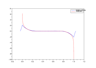
(a) Case where $n=4.10^{3}$, $\varepsilon=10^{-2}$, with width $\ell=0.2$

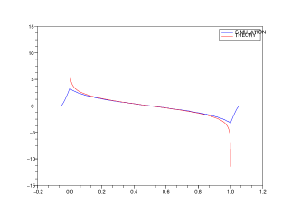
(b) Case where $n=4.10^{3}$, $\varepsilon=10^{-2}$, with width $\ell=0.9$

Figure 1. Perturbation of a uniform distribution by a standard band matrix: plot of the functions $F(\,\cdot\,)$ and $\frac{F_{D_{n}^{\varepsilon}}(\,\cdot\,)-F_{D_{n}}(\,\cdot\,)}{\varepsilon}$ (with $F_{D_{n}^{\varepsilon}}(\,\cdot\,)$ and $F_{D_{n}}(\,\cdot\,)$ the cumulative eigenvalue distribution functions of $D_{n}^{\varepsilon}$ and $D_{n}$) for different values of $\ell$.

2.2. Perturbation of the triangular pulse distribution by a GOE matrix

Let us consider the case where $\rho(x)=(1-|x|)\mathbbm{1}_{[-1,1]}(x)$ and $\sigma^{2}\equiv 1$ (what follows can be adapted to the case $\sigma^{2}(x,y)=\mathbbm{1}_{|y-x|\leq\ell}$, but the formulas are a bit heavy). In this case, thanks to the formula (9.6) of $H[\rho(\,\cdot\,)]$ given p. 509 of [11], we get

$$F(s)=(1-|s|)\mathbbm{1}_{[-1,1]}(s)\left\{(1-s)\log(1-s)-(1+s)\log(1+s)+2s\log|s|\right\}.$$

For small values of $\varepsilon$ and large values of $n$, the density $\rho_{\varepsilon}$ of the eigenvalue distribution $\mu_{\varepsilon}$ of $D^{\varepsilon}_{n}$ is approximately

$$\rho_{\varepsilon}(s)=\rho(s)+\varepsilon\frac{\partial}{\partial s}F(s)+o(\varepsilon),$$

which implies that the additive perturbation $\sqrt{\frac{\varepsilon}{n}}X_{n}$ alters the spectrum of $D_{n}$ by increasing the amount of eigenvalues in $[-1,-0.5]\cup[0.5,1]$ and decreasing the amount of eigenvalues around zero. This phenomenon is illustrated by Figure 2.

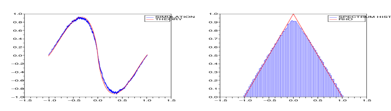
Figure 2. Perturbation of the triangular pulse distribution by a GOE matrix: Left: plot of the functions $F(\,\cdot\,)$ and $\frac{F_{D_{n}^{\varepsilon}}(\,\cdot\,)-F_{D_{n}}(\,\cdot\,)}{\varepsilon}$ (with $F_{D_{n}^{\varepsilon}}(\,\cdot\,)$ and $F_{D_{n}}(\,\cdot\,)$ the cumulative eigenvalue distribution functions of $D_{n}^{\varepsilon}$ and $D_{n}$). Right: plot of the eigenvalues histogram of $D_{n}^{\varepsilon}$ and of the spectral density $\rho$ of $D_{n}$. On the right figure, the (infinitesimal) increase of eigenvalues with respect to $\rho$ on $[-1,-0.5]\cup[0.5,1]$ and the (infinitesimal) decrease around zero can be observed, in agreement with the fact that, as the left figure shows, $F^{\prime}\gg 0$ on (approximately) $[-1,-0.5]\cup[0.5,1]$ and $F^{\prime}\ll 0$ around zero. Both figures were made with the same simulation ($n=6.10^{3}$ and $\varepsilon=10^{-2}$).

2.3. Free convolution with a semi-circular distribution and complex Burger’s equation

Let us consider the case where $\sigma^{2}\equiv 1$, which happens for example if the matrix $X_{n}$ is taken in the Gaussian Orthogonal Ensemble. In this case, by the theory of free probability developped by Dan Voiculescu (see e.g. [13] or [1, Cor 5.4.11 (ii)]), for all $t\geq 0$,

$$\mu_{{t}}=\mu\boxplus\lambda_{t},$$

where $\lambda_{t}$ is the semi-circular distribution with variance $t$, i.e. the distribution with support $[-2\sqrt{t},2\sqrt{t}]$ and density $\frac{1}{2\pi t}\sqrt{4t-x^{2}}.$ In this case, we know by the work of Biane [8, Cor. 2] that for all $t>0$, $\mu_{t}$ admits a density $\rho_{t}$. By the implicit function theorem, and the formula given in [8, Cor. 2], one easily sees that the function $(s,t)\longmapsto\rho_{t}(s)$ is regular. Then, by Theorem 1 and the fact that the linear span of $\mathcal{T}$ is dense in the set of continuous functions on the real line with null limit at infinity, one easily recovers the following PDE, which is a kind of projection on the real axis of the imaginary part of complex Burger’s equation given in [8, Intro.]

(3) $$\begin{cases}\frac{\partial}{\partial t}\rho_{t}(s)+\frac{\partial}{\partial s}\{\rho_{t}(s)H[\rho_{t}(\,\cdot\,)](s)\}=0,\\ \rho_{0}(s)=\rho(s).\end{cases}$$

For example, if $\mu=\lambda_{c}$ for a certain $c>0$, then by the semi-group property of the semi-circle distribution [1, Ex. 5.3.26], for all $t\geq 0$, $\mu_{t}=\lambda_{c+t}$ and $\rho_{t}(s)=\frac{1}{2\pi(c+t)}\sqrt{4(c+t)-s^{2}}$. One can then verify (3), using the formula (9.21) of $H[\rho_{t}(\,\cdot\,)]$ given p. 511 of [11].

Acknowledgements. It is a pleasure to thank Guy David for his useful advices about the Hilbert transform.

References

• [1] G. Anderson, A. Guionnet, O. Zeitouni. An Introduction to Random Matrices. Cambridge studies in advanced mathematics, 118 (2009).
• [2] G. Anderson, O. Zeitouni. A CLT for a band matrix model. Probab. Theory Related Fields 134 (2005), 283–338.
• [3] S.T. Belinschi. A note on regularity for free convolutions, Ann. Inst. H. Poincaré Probab. Statist. 42 (2006), no. 5, 635–648.
• [4] S.T. Belinschi. The Lebesgue decomposition of the free additive convolution of two probability distributions, Probab. Theory Related Fields 142 (2008), no. 1–2, 125–150.
• [5] S.T. Belinschi, D. Shlyakhtenko. Free probability of type B: analytic aspects and applications, to appear in American J. Math.
• [6] S.T. Belinschi, F. Benaych-Georges, A. Guionnet. Regularization by Free Additive Convolution, Square and Rectangular Cases. Complex Analysis and Operator Theory. Vol. 3, no. 3 (2009) 611–660.
• [7] H. Bercovici and D. Voiculescu. Regularity questions for free convolution, Nonselfadjoint operator algebras, operator theory, and related topics, 37–47, Oper. Theory Adv. Appl. 104, Birkhäuser, Basel, 1998.
• [8] P. Biane. On the Free convolution by a semi-circular distribution. Indiana University Mathematics Journal, Vol. 46, (1997), 705–718.
• [9] M. Février. Higher order infinitesimal freeness, arXiv.
• [10] M. Février, A. Nica. Infinitesimal non-crossing cumulants and free probability of type B, J. Funct. Anal. 258, 2983–2023 (2010).
• [11] F. W. King. Hilbert transforms. Vol. 2. Encyclopedia of Mathematics and its Applications, 125. Cambridge University Press, Cambridge, 2009
• [12] D. Shlyakhtenko. Random Gaussian band matrices and freeness with amalgamation. Internat. Math. Res. Notices 1996, no. 20, 1013–1025.
• [13] D. Voiculescu. Limit laws for random matrices and free products. Inventiones Mathematicae, 104 (1991) 201–220.