Fermi distribution of semicalssical non-eqilibrium Fermi states

Abstract

When a classical device suddenly perturbs a degenerate Fermi gas a semiclassical non-equilibrium Fermi state arises. Semiclassical Fermi states are characterized by a Fermi energy or Fermi momentum that slowly depends on space or/and time. We show that the Fermi distribution of a semiclassical Fermi state has a universal nature. It is described by Airy functions regardless of the details of the perturbation. In this letter we also give a general discussion of coherent Fermi states.

1. Introduction

Among various excitations of a degenerate Fermi gas, coherent Fermi states play a special role. A typical (not coherent) excitation of a Fermi gas consists of a finite number of holes below the Fermi level and a finite number of particles above it. Instead, a coherent Fermi state involves an infinite superposition of particles and holes arranged in such a manner that one can still think in terms of a Fermi sea (with no holes in it), the Fermi level of which depends on time and space.

Coherent states appear in numerous recent proposals about generating coherent quantum states in nanoelectronic devices and fermionic cooled atomic systems. These states can be used to transmit quantum information, test properties of electronic systems and to generate many-particles entangled states.

Coherent Fermi states can be obtained by different means. One is a sudden perturbation of the Fermi gas. For example, a smooth potential well, the spatial extent of which much larger than the Fermi length, is applied to a Fermi gas. Fermions are trapped in the well. Then the well is suddenly removed. An excited state of the Fermi gas obtained in this way is a coherent Fermi state. This kind of perturbation is typical for various manipulations with cooled fermionic atomic gases.

A realistic way to generate coherent Fermi states in electronic systems is by applying a time dependent voltage through a point contact, typifying many manipulations with nanoelectronic devices pointcontact ; Keeling .

Although the realization of coherent states in electronic systems experimentally is more challenging than in atomic systems, we will routinely talk about electrons.

From a theoretical standpoint coherent Fermi states are an important concept revealing fundamental properties of Fermi statistics. Coherent states appeared in other disciplines not directly related to electronic physics. Random matrix theory (RMT) Forrester-book , non-linear waves Miwa , crystal growth Spohn ; Okounkov , various determinental stochastic processes Johansson , asymmetric diffusion processes TASEP , to name but a few.

Unless a special effort is made (see e.g., pointcontact ) coherent Fermi states involve many electrons and are such that space-time gradients of the electronic density are much smaller than the Fermi scale. These state arise as a result of perturbing tye Fermi gas by a classical device. We call them semiclassical Fermi states. They are the main object of this paper. We will show that semiclassical Fermi states show great degree of universality as well as their single electron counterpart studied in pointcontact ; Keeling .

A general coherent Fermi state is a unitary transformation of the ground state $|0\rangle$ of a Fermi gas: $|U\rangle=U|0\rangle,\quad U=e^{i\int\Xi(x)\rho(x)dx-i\int\Pi(x)v(x)dx},$ where $\rho$ and $v$ are operators of electronic density and velocity $[\rho(x),\,v(y)]=-\frac{\hbar}{m}\nabla\delta(x-y)$ and $\Xi(x)$ and $\Pi(x)$ are two real functions characterizing the state Miwa ; Perelomov ).

For the purpose of this paper it is sufficient to assume that the motion of electrons is one dimensional and chiral (electrons move to the right), although most of the results we discuss are not limited to one-dimensional electronic gases. To this end, edge states in the Integer Quantum Hall effect may serve as a prototype. In a chiral sector the operators of density and velocity are identical $v|{\rm right}\rangle=\frac{\hbar}{m}\rho|{\rm right}\rangle$. The contribution of the right sector is easy to take into acoount. In this case the Fermi coherent state

$$|U\rangle=e^{i\int\Phi(x)\rho(x)dx}|0>$$ (1)

is characterized by a single function $\Phi$.

The function $\Phi$ can be undersstood as the action of an instantaneous perturbation by a potential $\hbar v_{F}\nabla\Phi(x)$, or, if we ignore the electronic dispersion the function $\Phi$ is the action of a time-dependent gate voltage $eV(t)=-\hbar\frac{d}{dt}\Phi(x_{0}-v_{F}t)$ applied through a point contact (located at $x_{0}$) .

Fermi coherent states feature inhomogeneous electric density $\rho(x)$ and current $I(x)$. Their expectation values give a meaning to the functions $\Xi$ and $\Pi$. In the chiral state, where the electric current and the electronic density are proportional, their expectation values are gradients of $\Phi$

$$\hbar\langle U|\rho(x)|U\rangle=\frac{\hbar}{ev_{F}}\langle U|I(x)|U\rangle=p_{F}+\hbar\nabla\Phi.$$ (2)

Consequently $\hbar\nabla\Phi(x)$ plays the role of the space-time modulation of the Fermi point, such that all states with momentum (or energy) less than $P_{F}(x)=\hbar\nabla\Phi(x)$ (or $E_{F}(x)=v_{F}\hbar\nabla\Phi$) are occupied (no holes in the Fermi sea) as shown in Fig. 1. We shall refer to the function $P_{F}(x)$ as the Fermi surface, with some abuse of nomenclature. We shall also term the region in phase space around $P_{F}(x)$ as the ’Fermi surf’.

The question we address in this letter is: what is the Fermi distribution in the ’Fermi surf’ of a modulated Fermi point, namely around and between extrema of $P_{F}(x)$?

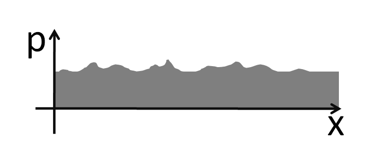
Figure 1: Modulated Fermi Edge. The Wigner function and Fermi number are almost 1 below the Edge (shaded area) and vanish above the Edge, having universal character in the ’surf’.

We will be especially interested in semiclassical Fermi states. These states involve many excited electrons. Its typical range is larger than the momentum spacing $\hbar\nabla\Phi\gg\Delta$ (but still is smaller than the Fermi momentum).

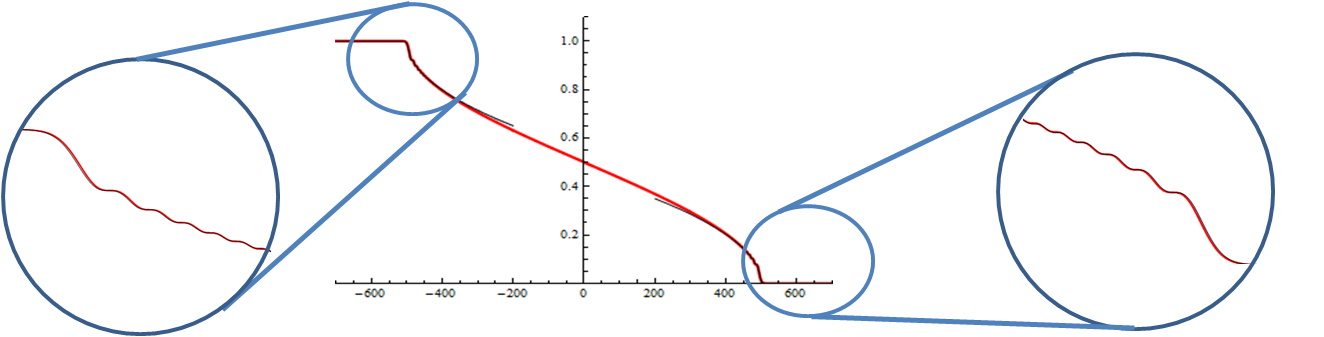
Figure 2: Universal asymptotes of the Fermi number. The graph (blue curve) shows the Fermi number in units of $\hbar/\ell$ for the example $\langle\rho(x)\rangle=\rho_{0}+(n/\ell)\cos(x/\ell)$ computed from Eq.(20). Black curves are the asymptotic forms obtained from the universal Fermi number formula (4). The universal asymptotes are magnified.

.

We show that, quite interestingly, the semiclassical Fermi surf features a universal Fermi distribution. There the Wigner function (11) is described by the function ${\rm Ai}_{1}(s)=\int_{s}^{\infty}{\rm Ai}(s^{\prime})ds^{\prime}$:

$$n_{F}(x,p+P_{F}(x))\approx{\rm Ai}_{1}\left(2^{2/3}\kappa p\right),$$ (3)

where the scale $\kappa=|\hbar^{2}P_{F}^{\prime\prime}(x_{*})/2|^{-1/3}$, and the offset $P_{F}(x)$ are the only information about the state that enters the formula. This formula holds close to any point where the Fermi surf is concave $P^{\prime\prime}_{F}(x)<0$. The Fermi occupation number (12) also displays universal behavior. Near a maxima, but well above the minima of the surf the Fermi number reads

$$n_{F}(P_{F}(x_{*})+p)\approx\kappa{\Delta}\left[\left[{\rm Ai}^{\prime}(\kappa p)\right]^{2}-(\kappa p){\rm Ai}^{2}(\kappa p)\right].$$ (4)

If the Fermi surf is convex rather than concave, then particle hole symmetry $n_{F}(p,x)\to 1-n_{F}(-p,x)$ provides the result for the Fermi number and Wigner function. Figures (1,2) illustrate the universal regimes. Here $\Delta$ is the momentum spacing ($2\pi\hbar/\Delta$ is the system volume).

The goal of the letter is twofold: to emphasize these simple, albeit universal, distributions, and, also to collect a few major facts about Fermi coherent states.

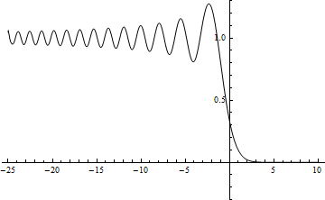
Figure 3: Universal behavior of the Wigner function vs. momentum for a concave Fermi surface obtained from (3).

2. Coherent Fermi states

The formal definition of a Fermi coherent states starts with the current algebra (see e.g., Stone (1994)). To simplify the discussion and formulas we consider only one chiral (right) part of the current algebra.

Current modes are Fourier harmonics of the electronic density $\rho(x)=\sum_{k>0}e^{\frac{i}{\hbar}kx}J_{k}$. An electronic current mode $J_{k}=\sum_{p}c^{\dagger}_{p}c_{p+k}$ (we count electronic momentum from the Fermi momentum $p_{F}$), creates a superposition of particle-hole excitations with momentum $k$. Positive modes annihilate the ground state, $|0\rangle$, a state where all momenta below $p_{F}$ are filled: $J_{k}|0\rangle=0,\quad k>0$. Negative modes are Hermitian conjugated to the positive modes $J_{-k}=(J_{+k})^{\dagger}$.

Chiral currents obey a current (or Tomonaga) algebra:

$$[J_{k},\,J_{l}]=\frac{k}{\Delta}\delta_{k+l,0}.$$ (5)

A Fermi coherent state $|U\rangle$ is defined as an eigenstate of positive current modes:

$$J_{k}|U\rangle=p_{k}|U\rangle,\quad k>0.$$ (6)

As follows from (1), $p_{k}=\Delta\int e^{-\frac{i}{\hbar}kx}d\Phi(x)/(2\pi)$ are positive Fourier modes of the function $\Phi(x)$. Assuming that the total number of particles in the coherent state is the same as in the ground state, or that the dc component of current is $I_{0}=\frac{ev_{F}}{\hbar}p_{F}$, i.e., $\int d\Phi=0$, we obtain

$$|U\rangle=Z^{-1/2}e^{\sum_{k>0}\frac{p_{k}}{k}J_{-k}}|0\rangle,\quad Z=e^{\sum_{k>0}\frac{1}{k}|p_{k}|^{2}}.$$ (7)

Using normal ordering with respect to the ground state (where all positive modes of the current are placed to the right of negative modes) the unitary operator reads :

$$e^{i\int\Phi(x)\rho(x)dx}=Z^{-\frac{1}{2}}\!:\!e^{i\int\Phi(x)\rho(x)dx}\!:=$$

$$=Z^{-\frac{1}{2}}e^{\sum_{k>0}\frac{1}{k}p_{k}J_{-k}}e^{-\sum_{k>0}\frac{1}{k}p_{-k}J_{k}}.$$ (8)

A coherent state represents an electronic wave-packet which is fully characterized by the electronic density. It is a simple exercise involving the algebra of the current operators to show that the function $\nabla\Phi(x)$ is a non-uniform part of the density as is in (2). Alternatively, one can use $Z$ as a generation function $\langle\rho(x)\rangle\equiv\langle U|\rho(x)|U\rangle=\rho_{0}+2{\rm Re}\sum_{k>0}ke^{ikx}\partial_{\bar{p}_{k}}\log Z$.

Coherent states obey the Wick theorem. The Wick theorem allows to compute a correlation function of any finite number of electronic operators, as a determinant over the one-fermionic function $K(x_{1},x_{2})\equiv\langle U|\psi^{\dagger}(x_{1})\psi(x_{2})|U\rangle$, where $\psi(x)=(\hbar/\Delta)^{1/2}\sum_{p}e^{\frac{i}{\hbar}px}c_{p}$ is an electronic operator. The one-fermionic function can be computed with the help of the formula:

$$U\psi(x)U^{-1}=e^{-i\Phi(x)}\psi(x)$$ (9)

which leads to the expression:

$$K(x_{1},x_{2})=\frac{e^{i\Phi(x_{1})-i\Phi(x_{2})-\frac{i}{\hbar}p_{F}(x_{1}-x_{2})}-1}{i(x_{1}-x_{2})},$$ (10)

valid for $\Delta|x_{1}-x_{2}|\ll\hbar$. An equivalent object appears in RMT where it is often called - Dyson’s kernel. We adopt this name. As points merge one recovers the density (2) $K(x,x)=\langle\rho(x)\rangle=\nabla\Phi$.

3. Wigner function and Fermi occupation number

The Wigner function is defined as Wigner transform of the Dyson kernel

$$n_{F}(x,p)=\frac{1}{2\pi}\int K(x+\frac{y}{2},x-\frac{y}{2})e^{-\frac{i}{\hbar}py}dy$$ (11)

The meaning of the Wigner function is clarified away from the surf. There it means an occupation of electrons in the phase space $(x,p)$: 1 below a surf, 0 above. On the surf Wigner function is not necessarily positive.

The Fermi number

$$n_{F}(p)=\langle U|c^{\dagger}_{p}c_{p}|U\rangle=\frac{\Delta}{2\pi\hbar}\int n_{F}(x,p)dx$$ (12)

is the Wigner function averaged over space.

Combining (10) and (11) we write

$$n_{F}(x,p)=\frac{1}{2\pi i}\int e^{\frac{i}{\hbar}\int^{x+\frac{y}{2}}_{x-\frac{y}{2}}\left(P_{F}(x^{\prime})-p\right)dx^{\prime}}\frac{dy}{y-i0}.$$ (13)

where we denoted $P_{F}(x)=\hbar\nabla\Phi=\langle\rho(x)\rangle$ as in (2).

Below we evaluate the integral (13) semiclassically bearing in mind that $\Phi$ is of a finite order as $\hbar\to 0$.

A universal regime arises at the Fermi surf, $\kappa|p-P_{F}(x)|\simeq 1$. In this case it is sufficient to expand $P_{F}(x)$ in a Taylor series around extrema of $P_{F}(x)$ to second order $P_{F}(x)=P_{F}(x_{*})+\frac{1}{2}P_{F}^{\prime\prime}(x_{*})(x-x_{*})^{2}+\dots$. Then the integral (13) becomes the Airy integral given in Eq. (3). Further integration over space yields (4).

In this regime the Dyson kernel in the momentum space $K_{p_{1},p_{2}}\equiv\langle U|c^{\dagger}_{p_{1}}c_{p_{2}}|U\rangle$ reads:

$$K_{p_{1},p_{2}}\approx\Delta\frac{{\rm Ai}(\kappa p_{1}){\rm Ai}^{\prime}(\kappa p_{2})-{\rm Ai}(\kappa p_{2}){\rm Ai}^{\prime}(\kappa p_{1})}{(p_{1}-p_{2})}$$ (14)

This is the celebrated Airy kernel appearing in numerous problems as the limiting shape of crystals Spohn , asymmetric diffusion TASEP , edge distribution of eigenvalues of random matrices Tracy and Widom (1994), etc.

The Fermi number (4) can be directly obtained from the kernel by taking a limit $p_{1}\to p_{2}$ in (14). At large positive momenta ($\kappa p\to+\infty$) the Fermi number behaves as $n_{F}(p)\sim\frac{\Delta}{8\pi p}e^{-\frac{4}{3}(\kappa p)^{3/2}}$ and as $\sim\frac{\Delta}{\pi}\left(\kappa\sqrt{-p\kappa}-\frac{1}{4p}\cos(\frac{4}{3}(-\kappa p)^{3/2})\right)$ for large negative momenta within the surf.

Away from the universal region of the surf the Fermi distribution can be computed within a saddle point approximation. The saddle point of the integral (13) is:

$$P_{F}(x+\frac{y}{2})+P_{F}(x-\frac{y}{2})=2p$$ (15)

It has pairs of solutions $\pm y_{*}(x,p)$. Let $P_{\rm max}=\max(P_{F}(x))$ and $P_{\rm min}=\min(P_{F}(x))$ be adjacent extrema of the surf. Without loss of generality we may assume that $(x,p)$ is outside the Fermi sea $p>P_{F}(x)$. The particle hole symmetry $n_{F}\to 1-n_{F}$ helps to recover the case when the momentum is inside the sea. If $p$ is in the surf, $p\in(P_{\rm min},P_{\rm min})$, then some saddle point pairs of (15) may be real. Their contribution produces oscillatory features with a suppressed amplitude. If $p$ hovers above the surf, $p>P_{\rm max}$, then the saddle points are imaginary. Their contributions are exponentially small.

Between two adjacent extrema the Wigner function reads:

$$n_{F}(x,p)\approx\sqrt{\frac{\hbar\left|\frac{dy_{*}}{dp}\right|}{8\pi|y_{*}|^{2}}}\times\left\{\begin{array}[]{lr}2\sin\left(\Omega-\frac{\pi}{4}\right),&p\in(P_{\rm min},P_{\rm max})\\ e^{-|\Omega|},&p>P_{\rm max},\\ \end{array}\right.$$ (18)

where $\hbar\Omega=-\int_{P_{F}(x)}^{p}y_{*}(x,p^{\prime})dp^{\prime}$. In the surf it is half the action of a semiclassical periodic orbit - the area of the graph $y_{*}(x,p)$ vs $p$. In the universal regime, when one approximates $y_{*}(x,p)\approx\hbar\kappa^{3/2}\left(p-P_{F}(x)\right)^{1/2}$ this equation reproduces asymptotes of Eq.(3): $n_{F}(x,p+P_{F}(x))\sim(8\pi)^{-1/2}(\kappa p)^{-3/4}e^{-3(\kappa p)^{3/2}}$.

A Fermi coherent state with a periodic current is an instructive example. It corresponds to ”quantum pumping” - periodic transfer a charge through the system by applying a periodic voltage through a point contact. Setting $\langle\rho(x)\rangle=\rho_{0}+(n/\ell)\cos(x/\ell)$ the Dyson kernel in the momentum representation becomes the integer Bessel kernel

$$K_{p_{1},p_{2}}=\frac{n}{2}\frac{m_{1}J_{m_{1}}(n)J_{m_{2}}^{\prime}(n)-m_{2}J_{m_{2}}(n)J_{m_{1}}^{\prime}(n)}{m_{1}-m_{2}},$$ (19)

where $p_{1,2}=\hbar m_{1,2}/\ell$, where $m_{1}\neq m_{2}$ are integers. The Fermi number is given by ($m_{F}=p_{F}\ell/\hbar$):

$$n_{F}(p)=\frac{1}{2}-{\rm sign}(p)\left[\frac{J_{0}^{2}(n)}{2}+\sum_{m=1}^{m_{F}}J_{m}^{2}(n)\right].$$ (20)

This formula allows to compare the asymptotes near the edges to the universal expression above. Using the homogeneous asymptote of Bessel function $J_{m}(m-(m/2)^{1/3}\zeta)\sim(2/m)^{1/3}{\rm Ai}(\zeta)$ at large $m$, one recovers (14) and (4). Fig. 2 illustrates the universal asymptote.

4. Holomorphic Fermions as coherent states

To contrast semiclassical coherent Fermi states and quantum coherent Fermi states, we briefly discuss special coherent states known as holomorphic fermions Miwa1 .

Holomorphic fermions are defined as a superposition of fermionic modes $\psi(z)=\sum_{p}e^{\frac{i}{\hbar}pz}c_{p}$, with a complex ”coordinate” ${\rm Im}z<0$.

Holomorphic fermions are coherent states since they can be represented as an exponent of a Bose field - displacement of electrons $\varphi(z)=\sum_{k\neq 0}\frac{\Delta}{ik}e^{\frac{i}{\hbar}kz}J_{k}$ Miwa ; Stone (1994)

$$\psi(z)=c_{p_{F}}:e^{i\varphi(z)}:$$ (21)

A function $\Phi$ for a string of fermions $\prod_{i=1}^{n}\left(\psi^{\dagger}(z_{i})\psi(\zeta_{i})\right)|0\rangle$ is $e^{i\Phi(x)}=\prod_{i=1}^{n}\frac{x-z_{i}}{x-\bar{z}_{i}}\frac{x-\bar{\zeta}_{i}}{x-\zeta_{i}}$. The density (or current) of these states consists of Lorentzian peaks, each carrying a unit electronic (positive/negative) charge $\langle\rho(x)\rangle-\rho_{0}=\sum_{i}{\rm Im}\,\left(\frac{1}{x-z_{i}}-\frac{1}{x-\zeta_{i}}\right)$, so that the state is a set of single electronic pulses. For a possible applications of these states in nano-devices see Keeling ; pointcontact . As the complex coordinate approaches the real axis $\zeta=x-i0$ a holomorphic fermion operator becomes an electronic operators $\psi(z)\to\psi(x)$ as its density becomes a delta-function.

Coherent states formed by a single holomorphic fermion carries a unit charge in contrast to semiclassical Fermi states. The Wigner function of this state follows from (10)

$$n_{F}(x,p)=\frac{1}{2\pi i}\int\frac{x+\frac{y}{2}-z}{x+\frac{y}{2}-\bar{z}}\frac{x-\frac{y}{2}-\bar{z}}{x-\frac{y}{2}-z}e^{-\frac{i}{\hbar}py}\frac{dy}{y-i0},$$

where $z=X-ia$, $X$ is a real coordinate of fermion and $a$ is its width ($a\Delta\ll\hbar$) . $a$ is positive for an annihilation operator and negative for a creation operator. Evaluating this integral we obtain

$$n_{F}(x,p)=\Theta(-p)-\Theta(-pa)a\frac{\sin 2p(x-X)}{x-X}e^{\frac{2}{\hbar}pa},$$

$$n_{F}(p)=\Theta(-p)-\Theta(-pa)\frac{2a\Delta}{\hbar}e^{\frac{2}{\hbar}pa},$$ (22)

Noticeable features of this distribution are: the Fermi function jumps on the Fermi edge; beyond the Fermi edge, the Fermi number and the Wigner functions decay exponentially, if $a>0$ a holomorphic fermion $\psi(z)$ acts like an annihilation operator removing particles from Fermi edge (vice versa if $a<0$); the Wigner function features Friedel’s type oscillation with a distance $x-X$ to the center of the fermion.

6. Fermi coherent states and Random Matrix Ensembles.

We complete the letter by a brief discussion of the relation to the theory of Random Matrices.

Consider $n$ electrons from the ground state of the Fermi gas in positions $x_{1},\dots,x_{n}$. We write this state as $\langle x_{1},\dots,x_{n}|=\langle 0|c^{\dagger}_{p_{F}}\dots c^{\dagger}_{p_{F}-n}\psi(x_{1})\dots\psi(x_{n})$, where we set momentum spacing to 1 for brevity. Let us ask for the probability to find this state in the coherent state $|U\rangle$. It is $|\Psi(x_{1},\dots,x_{n})|^{2}$, where $\Psi(x_{1},\dots,x_{n})=\langle x_{1},\dots,x_{n}|U\rangle/\langle 0|U\rangle$.

Fermions in coherent states obey the Wick theorem: a matrix element of a particle-hole string inserted between two (generally different) coherent states is a Slater determinant built out of particle-hole matrix element. In particular $\Psi(x_{1},\dots,x_{n})={\rm det}\left(\Psi_{p_{F}-l}(x_{m})\right)_{l,m\leq n}$ is a Slater determinant of a single particle matrix element $\Psi_{p_{F}}(x)=\langle 0|c^{\dagger}_{p_{F}}\psi(x)|U\rangle/\langle 0|U\rangle$. We compute it with the help of the current algebra and bosonic representation (21). Up to a normalization

$$\Psi_{p}(x)\sim e^{-\frac{1}{\hbar}Y_{p}(x)}.$$ (23)

This formula features the complex curve $Y_{p}(z)=-ipz+\sum_{k>0}\frac{\hbar}{k}p_{k}e^{\frac{i}{\hbar}kz}$, a useful characteristic of the coherent state. The function $Y_{p}(z)+ipz$ is analytic in the upper half-plane. Its boundary value on the real axis is

$$Y_{p}(x)+ipx=\frac{\hbar}{2}\left(V(x)-i\Phi(x)\right)=i\hbar\sum_{k>0}\frac{p_{k}}{k}e^{\frac{i}{\hbar}kx},$$ (24)

where $V(x)$ and $\Phi(x)$ are real and imaginary part of the boundary value of the analytic function. They are connected by the Hilbert transform.

For example, a complex curve for a pumping considered in Sec. 3 is $Y_{p}(z)=-ipz+\frac{\hbar n}{2\ell}e^{\frac{z}{\ell}}$. In the case of a string of fermions the curve is $Y_{p}(z)=-ipz+\hbar\sum_{i=1}^{n}\log\frac{z-\bar{\zeta}_{i}}{z-\bar{z}_{i}}$.

Computing the Slater determinant of (23) we obtain

$$\Psi(x_{1},\dots,x_{n})=Z_{n}^{-1/2}e^{-\frac{1}{\hbar}\sum_{i=1}^{n}(Y(x_{i})-ip_{F}x_{i})}\Delta(x),$$ (25)

where $\Delta(x)=\mbox{det}\,\left(e^{\frac{i}{\hbar}px_{l}}\right)_{p,l\leq n}=\prod_{i>j}\left(e^{\frac{i}{\hbar}x_{i}}-e^{\frac{i}{\hbar}x_{j}}\right)$ is the VanderMonde determinant.

The normalization factor in (25)

$$Z_{n}=\int\prod_{n\geq i>j\geq 1}|e^{\frac{i}{\hbar}x_{i}}-e^{\frac{i}{\hbar}x_{j}}|^{2}\prod_{i=1}^{n}e^{-V(x_{i})}dx_{i}$$ (26)

is the the partition function of eigenvalues of a circular unitary $n\times n$-matrix Forrester-book . At the limit of vanishing spacing one replaces $e^{\frac{i}{\hbar}x}\to 1+i\hbar x$. In this case coherent Fermi state is described by Random Hermitian Matrix ensemble.

If $n$ is large, Eq. (25) can be interpreted as a coordinate representation of the coherent state. A Fermi coherent state may be thought as a Fermi sea filled by particles (without holes) with wave functions (23) and $p=1,\dots,n$. The coordinate representation provides another avenue to compute matrix elements discussed in this paper as a limit $n\to\infty,\,p_{F}/n\to\infty$. Some of them have been studied for various reasons in the theory of Random Matrix Ensembles (see e.g., Brezin:Zee for derivation of the Dyson kernel).

References

- (1) D. A. Ivanov, H. W. Lee and L. S. Levitov Phys. Rev. B. 56 (1997), 6839 J. Keeling, I. Klich and L. Levitov Phys. Rev. Lett. 97 (2006), 116403; J. Keeling, A. V. Shytov, and L. S. Levitov ibid 101 (2008), 196404
- (2) G. F‘eve, et al., Science 316 (2007), 1169
- (3) P. J. Forrester, Log-Gases and Random Matrices (LMS-34), Princeton University Press, 2010
- (4) Solitons: differential equations, symmetries and infinite dimensional algebras By Tetsuji Miwa, Michio Jimbo, Etsuro Date, Cambridge Acad. Press, 2000
- (5) P. L. Ferrari, H. Spohn, J. Stat. Phys., 113 (2003), 1
- (6) A. Okounkov and N. Reshetikhin, J. Amer. Math. Soc., 16 (2003), 581
- (7) K. Johansson, Random matrices and determinantal processes, Lecture Notes of the Les Houches Summer School 2005 (A. Bovier at all eds.), Elsevier Science, 2006, p. 1
- (8) A. Borodin, P.L. Ferrari, and T. Sasamoto, Comm. Math. Phys. 283 (2008), 417449
- (9) For coherent states for finite dimensional fermionic system see A.Perelomov, Generalized Coherent States and Their Applications, Springer, Berlin, 1986
- (10) E. Bettelheim, A. G. Abanov, P. Wiegmann J. Phys. A: Math. Theor. 41 (2008), 392003
- Stone (1994) M. Stone, ed., Bosonization (World Scientific, Singapore, Singapore, 1994)
- Anderson (1967) P. W. Anderson, Phys. Rev. Lett. 18, 1049 (1967)
- Tracy and Widom (1994) C. A. Tracy and H. Widom, Commun. Math. Phys. 159, 151 (1994)
- (14) In mathematical literature holomorphic fermions have been introduced in Miwa . For some physical applications including shot noise of these states, see recent papers Keeling
- (15) E. Brezin and A. Zee, Nucl. Phys. B 402, 613 (1993)