Black hole solutions in string theory

Abstract

Supersymmetric solutions of supergravity have been of particular importance in the advances of string theory. This article reviews the current status of black hole solutions in higher-dimensional supergravity theories. We discuss primarily the gravitational aspects of supersymmetric black holes and their relatives in various dimensions. Supersymmetric solutions and their systematic derivation are reviewed with prime examples. We also study the stationary or dynamically intersecting branes in ten and eleven-dimensions, which provide a number of interesting black objects via the dimensional reduction and duality transformations.

KEK-TH 1453

1 Introduction

Gravitational physics in higher dimensions has played and will continue to play a central rôle in the development of string theory as well as phenomenological predictions of brane world scenarios. Among other things, a various kinds of interesting higher-dimensional “black objects” have been found and extensively studied over the last two decades. These black objects exhibit much richer physical properties–even in the vacuum case–than the four-dimensional counterparts[1]. One of the most exciting findings is the discovery of a black ring [2, 3], which describes an asymptotically flat regular black “hole” with topology $S^{1}\times S^{2}$. Since there also exists an ordinary rotating spherical black hole [4] with the same mass and angular momentum as the ring in a certain range of parameters, it exemplified the end of black-hole uniqueness in higher dimensions and have triggered intensive works on higher dimensional gravity[1]. Another novel phenomenon intrinsic to higher dimensions is the dynamical gravitational instability of black branes [5, 6]. This instability provides a considerably rich phase diagram with new insights, such as non-uniqueness, topology changing phase transitions between black objects [7, 8] and new kind of black holes with pinched horizons [9].

Brane configurations in supergravity are much more relevant to string theory as a low energy description of D-branes. Since these black branes preserve some fraction of supersymmetries, we are able to bring their behavior in the strongly coupled regime under some control. Supersymmetric configurations often circumvent instability and have non-renormalization properties [10], which are not applicable for non-supersymmetric ones. A principal achievement of the study of supersymmetric black holes is the microscopic derivation of Bekenstein-Hawking entropy [11, 12] exploiting the D-brane technology [13]. String theory promoted the conjecture of Bekenstein about the striking resemblance between black-hole mechanics and ordinary thermodynamics [11, 14] to more than an analogy. A number of subsequent developments since the pioneering work of Strominger & Vafa [13] have witnessed a significant progress in the statistical description of black hole entropy and highlighted the utility of supersymmetric intersecting brane configurations (see Ref. [15] for a review).

In this article, we shall review black holes in supergravity theories. Since these studies are extremely broad in scope ranging from the phenomenological topic to the basis of AdS/CFT-correspondence [16], it is almost impossible to cover all aspects. So we shall stick to the discussion of gravitational physics of various higher-dimensional supersymmetric black holes and their cousins, with an emphasis on the distinction from four-dimensional ones and from the non-supersymmetric ones.

The organization of the rest of the paper is as follows. In the next section we shall make a brief overview of supersymmetric black holes in four dimensions. Section 3 is devoted to the classification of supersymmetric solutions. Focusing mainly on the five dimensions, we will study some black hole solutions. In section 4, the intersecting black brane solutions with rotations are discussed, which produce upon dimensional reduction various kinds of lower dimensional black holes. The extension to the dynamical background is examined in section 5. It is shown that the dimensional reduction of these time-dependent branes provides black holes in an expanding Friedmann-Lemaîtle-Robertson-Walker (FLRW) universe, on which the standard cosmological evolutionary scenario is based. Section 6 concludes with several remarks.

We shall work with mostly plus metric signature. The convention of the Dirac matrix $\gamma_{\mu}$ is $\bar{\psi}:={\rm i}\gamma^{0}\psi^{\dagger}$. The four-dimensional chiral matrix is given by $\gamma_{5}=i\gamma_{0123}$.

2 Supersymmetric black holes: a retrospective

2.1 A Bogomol’nyi bound

Since the gravitational energy is negative due to the universally attractive nature of gravity, it is not a priori clear whether the total energy of the system is positive. Thus, the establishment of the positive energy theorem is one of the most sensational breakthroughs in mathematical theory of relativity. Stated precisely, the Arnowitt-Deser-Misner (ADM) energy [17] of an asymptotically flat spacetime must be non-negative under the dominant energy condition, and vanishes only for the flat spacetime. The first proof given by Schoen and Yau [18] is based on the variations of the extremal surfaces. A completely different but extremely simple proof was given by Witten [20] and later refined by Nester [21]. A notable feature of Witten’s argument is that the ADM momentum is expressed in terms of an auxially spinor field $\epsilon$. The use of the spinor field was originally motivated by an attempt to construct quantum theory of supergravity. Nevertheless, Gibbons and Hull [22] demonstrated that its origin can be found within the classical regime of supergravity. They considered the four-dimensional $N=2$ supergravity, whose bosonic sector is the Einstein-Maxwell theory, and obtained a stronger inequality

$$M\geq\sqrt{Q^{2}+P^{2}}\,,$$ (1)

where $M$ is the ADM energy, $Q$ and $P$ correspond to the total electric and magnetic charges, respectively. In the context of supergravity, they enter the supersymmetry algebra as central charges:

$$\{\mathbf{Q},\mathbf{Q}^{*}\}=i\gamma^{\mu}CP_{\mu}+(Q+i\gamma_{5}P)C\,,$$ (2)

where $C$ is the charge conjugation matrix, $\mathbf{Q}$ is the Dirac supercharge and $P_{\mu}$ is the ADM four momentum with $M=\sqrt{-P^{\mu}P_{\mu}}$. The ADM energy and the electromagnetic charges are all defined by surface integrals at infinity. The above equation (2) manifests that the Witten-Nester expression of ADM energy is obtained by the repeated supersymmetry transformations generated by an associated Noether charge. [23].

The inequality (1) is reminiscent of the Bogomol’nyi-Prasad-Sommerfield (BPS) bound for solitonic objects. In the context of gauge theory, it is known that the solitonic configuration saturating this bound fulfills a certain kind of 1st-order differential equations. Furthermore multiple configurations of solitons are allowed. This is attributed to a delicate balance of forces between the electromagnetic repulsion and the attractive force caused by other fields, e.g., a scalar field. The BPS objects are stable classically, and in the supersymmetric case they are even stable quantum mechanically [10]. The number of BPS states does not change if coupling constants are varied continuously, since it is essentially a topological invariant quantity. This is the key ingredient characterizing the non-perturbative nature of BPS states.

The inequality (1) implies that the same argument carries over to the gravitating system. It is known that the lower bound is attained, or equivalently the matrix $\{\mathbf{Q},\mathbf{Q}^{*}\}$ is not of the maximal rank, if and only if the asymptotically flat spacetime admits a spinor $\epsilon$ satisfying the analogue of first-order BPS equation [22]

$$\hat{\nabla}_{\mu}\epsilon:=\left(\nabla_{\mu}+\frac{i}{4}F_{\nu\rho}\gamma^{\nu\rho}\gamma_{\mu}\right)\epsilon=0\,.$$ (3)

This can be viewed as the vanishing of gravitino supersymmetry transformation $\delta_{\epsilon}\psi_{\mu}=\hat{\nabla}_{\mu}\epsilon=0$, which leaves the bosonic background invariant (note that $\epsilon$ is anti-commuting in this context, whereas it is taken to be commuting in the proof of positive energy theorem). Since the BPS equation (3) is the 1st-order linear differential equation, supersymmetric solutions are very simple and expected to inherit properties of instantons.

It is worthwhile to note that the integrability of the Killing spinor equation allows us to relate the BPS geometries admitting a Killing spinor to those solving equations of motion. Acting a supercovariant derivative to Eq. (3) and anti-symmetrizing the indices, one obtains $\hat{\nabla}_{[\mu}\hat{\nabla}_{\nu]}\epsilon=0$. Contracting this with $\gamma^{\nu}$, using $\nabla_{[\mu}\nabla_{\nu]}\epsilon=(1/8)R_{\mu\nu\rho\sigma}\gamma^{\rho\sigma}\epsilon$ and the Bianchi identity $R_{\mu[\nu\rho\sigma]}=0$, it is a simple exercise to obtain

$$\left[E_{\mu\nu}\gamma^{\nu}+\frac{i}{2}\left(\gamma^{\nu\rho\sigma}\gamma_{\mu}\nabla_{[\nu}F_{\rho\sigma]}-2\gamma_{\nu}\gamma_{\mu}\nabla_{\rho}F^{\nu\rho}\right)\right]\epsilon=0\,,$$ (4)

where $E_{\mu\nu}:=R_{\mu\nu}-2(F_{\mu\rho}{F_{\nu}}^{\rho}-\tfrac{1}{4}F^{2}g_{\mu\nu})$ and its vanishing is equivalent to the Einstein equations. If the Maxwell equations and the Bianchi identity for the Maxwell field are satisfied, the last two terms in Eq. (4) drop off, giving $E_{\mu\nu}\gamma^{\nu}\epsilon=0$. Contracting this with $\bar{\epsilon}$ and $E_{\mu\rho}\gamma^{\rho}$, we obtain

$$E_{\mu\nu}V^{\nu}=0\,,\qquad E_{\mu\nu}{E_{\mu}}^{\nu}=0\quad(\textrm{no sum on $\mu$}).$$ (5)

It is clear that $V^{\mu}=i\bar{\epsilon}\gamma^{\mu}\epsilon$ cannot be spacelike since we have $V^{0}=\epsilon^{\dagger}\epsilon>0$ for a nonvanishing spinor $\epsilon$ satisfying Eq. (3). In the case where $V^{\mu}=i\bar{\epsilon}\gamma^{\mu}\epsilon$ is timelike, the first equation means that $E_{00}=E_{0i}=0$ and the second equation implies that $E_{ij}=0$ (in an obvious orthonormal frame), as we desired. In the null case solving only the component $E_{++}=0$ (in the basis $V=e^{+}$) suffices to ensure that other components of Einstein’s equations automatically follow. Conversely, the integrability condition can be used to check consistency for the 1st-order equation [24].

Although supersymmetric solutions are characterized by the BPS relation, there is no general proof that any theories admit the Bogomol’nyi bound applied to non-supersymmetric solutions. Ref. [25] investigated circumstances under which one can derive the bound (à la Witten-Nester), and found that this is the case only for the solutions of bosonic sector of supergravity. This fact also validates the stability of supersymmetric solutions with a fair amount of certainty.

2.2 Supersymmetric black holes in four dimensions

An illustrative example of the supersymmetric solution is the Majumdar-Papapetrou solution [26]. Let us begin by the electrically charged extremal Reissner-Nordström solution with the ADM mass $M=Q$. In the isotropic coordinates, the solution is given by

$${\rm d}s^{2}_{4}=-\left(1+\frac{Q}{r}\right)^{-2}{\rm d}t^{2}+\left(1+\frac{Q}{r}\right)^{2}\left({\rm d}r^{2}+r^{2}{\rm d}\Omega_{2}^{2}\right)\,,\qquad A=\frac{{\rm d}t}{1+Q/r}\,,$$ (6)

where ${\rm d}\Omega_{2}^{2}$ is the line element of a unit two-sphere. Observing that the term $1+Q/r$ describes a monopole harmonic on the Euclid 3-space $\mathbb{R}^{3}$, it is shown that any harmonic on the flat 3-space still solves the Einstein equations, yielding the Majumdar-Papapetrou solution

$${\rm d}s_{4}^{2}=-H^{-2}{\rm d}t^{2}+H^{2}{\rm d}\vec{x}^{2}\,,\qquad A=H^{-1}{\rm d}t\,,$$ (7)

where $H$ is independent of $t$ and satisfies the Laplace equation $\vec{\nabla}^{2}H=0$. Here and hereafter, 3-dimensional vector notation will be used for quantities on $\mathbb{R}^{3}$. The Majumdar-Papapetrou solution (7) is indeed supersymmetric since it admits a nonzero Killing spinor $\epsilon=H^{-1/2}\epsilon_{\infty}$ satisfying Eq. (3), where $\epsilon_{\infty}$ is a constant spinor satisfying $i\gamma^{0}\epsilon_{\infty}=\epsilon_{\infty}$. Since the matrix $\gamma^{0}$ has eigenvalues $\pm i$ coming in pairs, this projection breaks half of the supersymmetries of vacuum. For the multi-centered harmonics,

$$H=1+\sum_{k=1}^{N}\frac{Q_{k}}{|\vec{x}-\vec{x}_{k}|}\,,$$ (8)

the solution describes $N$ charged black holes in static equilibrium [27], where $Q_{k}$ represents the individual charge of the point mass $M_{k}=Q_{k}$ positioned at $\vec{x}=\vec{x}_{k}$. The ADM mass is equal to the total charge $Q=\sum_{k}Q_{k}$, which saturates the BPS bound (1) as expected.

One may follow the same steps for the rotating spacetime. Let us consider the Kerr-Newman solution with $M=Q$, the metric of which reads

$${\rm d}s_{4}^{2}= -\frac{\rho^{2}}{\Sigma^{2}}\left[{\rm d}t+\frac{aQ(2r+Q)\sin^{2}\theta}{\rho^{2}}{\rm d}\phi\right]^{2}+\frac{\Sigma^{2}}{\rho^{2}}\left[\rho^{2}\left(\frac{{\rm d}r^{2}}{\Delta}+{\rm d}\theta^{2}\right)+\Delta\sin^{2}\theta{\rm d}\phi^{2}\right]\,,$$ (9)

with

$$\Sigma^{2}=(r+Q)^{2}+a^{2}\cos^{2}\theta\,,\quad\Delta=r^{2}+a^{2}\,,\quad\rho^{2}=r^{2}+a^{2}\cos^{2}\theta\,,$$ (10)

where the radial coordinate $r$ has been shifted by $Q$ from the conventional Boyer-Lindquist coordinates. Since $g^{rr}>0$ for $a\neq 0$, the rotating spacetime (9) describes a naked singularity rather than a black hole. The cosmic censorship bound does not necessarily coincide with the Bogomol’nyi bound. Nonetheless, this metric is still supersymmetric and of great help to appreciate the rôle of rotation.

It is easy to verify that the 3-metric in square brackets in Eq. (9) corresponds to the flat Euclid space. One can also find that $V=1+Q/(r-ia\cos\theta)$ is a complex harmonic function on $\mathbb{R}^{3}$ with an imaginary part being the rotation. These observations lead us to obtain a more general class of solutions called an Israel-Wilson-Perjés (IWP) family [28],

$${\rm d}s_{4}^{2}=-|V|^{-2}({\rm d}t+\omega)^{2}+|V|^{2}{\rm d}\vec{x}^{2}\,,\qquad\vec{\nabla}\times\vec{\omega}=2{\rm Im}(\bar{V}\vec{\nabla}V)\,,$$ (11)

where $V$ is an arbitrary complex harmonic on $\mathbb{R}^{3}$ and $\omega$ is obtained by quadrature. This enables us to generate a solution of the multiple Kerr-Newman objects by superposition. These specific supersymmetric backgrounds give us a lot of physical implications.

Let us summarize here a list of our heuristic knowledge about supersymmetric solutions:

Force balance:  The Majumdar-Papapetrou metric (7) realizes finely the force balance because the the Maxwell field is responsible for maintaining the black holes apart. This is most explicitly illustrated by the complete linearity of the field equation $\vec{\nabla}^{2}H=0$. The IWP solution (11) also restores the no force condition $\vec{\nabla}^{2}V=0$. Supersymmetric gravitating solutions are in mechanical equilibrium just as those in gauge theories.

Zero Hawking temperature:  All known supersymmetric solutions describing a regular black hole have degenerate horizons as for the extreme Reissner-Nordström solution. This means that the Hawking temperature [12] (i.e., the surface gravity of the horizon) vanishes. Remark that the zero temperature black holes are not always supersymmetric, e.g., the extremal Kerr(-Newman) is not BPS. This is fairly persuasive since the inside region of the nonextremal black holes is dynamical, which is not compatible with the mechanical equilibrium. For instance, the Schwarzschild interior describes a Kantowski-Sachs cosmology [29]. From the gravitational point of view, degenerate horizons are exceptional and believed to be unrealized via the gravitational collapse due to the cosmic censorship conjecture [30]. These configurations are ideal ground states of the theory.

Since the zero-temperature black hole does not radiate thermal quanta, it cannot be unstable by spontaneous creation of particles. Moreover, the superradiant loss of charge is not permissible in the $N=2$ supergravity, since there are no elementary charged particles in this theory. This validates the solitonic character of BPS objects.

No ergoregion:  For the Kerr-Newman metric with $M=Q$ (9) and the IWP solution (11), it is obvious that $g_{tt}<0$ is always satisfied. This means that the solution fails to posses an ergoregion even if the spacetime has nonvanishing angular momentum. It is easy to verify that the ergoregion does not exist in the Kerr-Newman family only when $M=Q$. Thus, the asymptotically flat rotating BPS objects are free from a superradiant instability. That kind of a dynamical process does not occur in a supersymmetric background.

Near-horizon geometry:  In the vicinity of each point source $\vec{x}\sim\vec{x}_{k}$ in the Majumdar-Papapetrou solution, one can drop the constant term from the harmonic $H$. Then the Majumdar-Papapetrou metric (7) is approximated by the ${\rm AdS}_{2}\times S^{2}$ geometry with the same curvature radii $Q_{k}$. This means that each degenerate horizon is locally isometric to the neighbourhood of that of ${\rm AdS}_{2}$ [31]. Taking this limit, the novel isometry group ${\rm SO}(2,1)$ appears. A more relevant aspect here is that the ${\rm AdS}_{2}\times S^{2}$ spacetime preserves the maximal set of Killing spinors, i.e., it is a maximally supersymmetric background to the Einstein-Maxwell theory [32]. It follows that the Majumdar-Papapetrou metric connects two different vacua: the Minkowski spacetime at infinity and ${\rm AdS}_{2}\times S^{2}$ near the horizon. This property is also analogous to ordinary solitons which separate two distinct vacua.

These properties have been confirmed for a number of black hole systems in various (ungauged) supergravity theories. To reach a further conviction that these features are indeed universal to all supersymmetric black holes, a more systematic study of supersymmetric solutions is desirable. The above ad hoc steps or ansatz-based approaches are inadequate to uncover general properties of supersymmetric solutions.

A first progression in this direction was made by Tod. [33] He assumed the existence of at least one Killing spinor $\epsilon$ satisfying Eq. (3) and considered bilinears built out of the Killing spinor. These tensorial quantities fulfill many algebraic and differential constraints, which are sufficient to reconstruct full bosonic elements of the theory. The BPS solutions fall into two classes–timelike and null family–depending on whether the Killing vector $V^{\mu}=i\bar{\epsilon}\gamma^{\mu}\epsilon$ constructed from the Killing spinor is timelike or null. The general metric of timelike class is given by the IWP family, whilst the null family is described by the plane-fronted wave with parallel rays [29]. Therefore the result in $D=4$, $N=2$ supergravity is fairly simple: the supersymmetric black-hole configurations are exhausted by the Majumdar-Papapetrou solution since the regular horizons are destroyed by rotation. This is attributed to that the condition for the degenerate horizon reads $M=M(Q,J)$, whereas the Bogomol’nyi bound (3) does not involve $J$. This property appears common to every (ungauged) supergravity theory in four dimensions [35]. Additional matter sources such as dilaton [36, 24] and axion ($N=4$ supergravity) [36, 37] do not produce a regular rotating black hole in an asymptotically flat spacetime.

3 Classification of supersymmetric solutions

Although Tod’s work has thrown new light on the classification programme of supersymmetric solutions in supergravity, a new technique is required in higher dimensions since the Newman-Penrose formalism was fully used therein. Recently, Gauntlett et al. [38] have successfully classified all the supersymmetric solutions of five-dimensional minimal supergravity by making use of Killing spinor bilinears (see Ref. [39] for an early study along this line). This seminal work has provided us with the wide range of applications. Thereafter the classification program has achieved a remarkable development in diverse supergravities in various dimensions [40, 41, 42, 43, 44, 45, 46, 35, 47]. It has been revealed that higher-dimensional supersymmetric solutions exhibit a considerably rich spectrum and allow physically interesting nontrivial black objects with rotations.

3.1 Five dimensional minimal supergravity

The simplest model is the minimal supergravity in five dimensions [38], which admits the same number of supercharges as in $D=4$, $N=2$ supergravity. The bosonic sector of five-dimensional minimal supergravity constitutes the Einstein-Maxwell theory with the Chern-Simons term. The action is given by

$$S_{5}=\frac{1}{16\pi G_{5}}\int\left({}^{(5)}R*1-2F\wedge*F-\frac{8}{3\sqrt{3}}A\wedge F\wedge F\right)\,,$$ (12)

where $F={\rm d}A$ is the ${\rm U}(1)$ gauge field strength, $\wedge$ is the wedge product and $*$ is the Hodge dual operator. This theory arises via a consistent truncation of toroidal compactification of eleven-dimensional supergravity. The Chern-Simons term contributes when the solution has both of the electric and magnetic parts.

The strategy for classifications of supersymmetric solutions is parallel to Tod’s argument: assume the existence of a Killing spinor, construct its bilinear quantities and derive algebraic and differential constraints which they obey.

From a pair of (commuting) symplectic-Majorana spinors $\epsilon^{1}$ and $\epsilon^{2}$, we can define a scalar $f$, a vector $V_{M}$ and three 2-forms $J^{(i)}_{MN}$ $(i=1,2,3)$ by

$$f=\bar{\epsilon}^{1}\epsilon^{2}\,,\quad V_{M}=i\bar{\epsilon}^{1}\gamma_{M}\epsilon^{2}\,,\quad J^{(1)}_{MN}=\frac{1}{2}(\bar{\epsilon}^{1}\gamma_{MN}\epsilon^{1}+\bar{\epsilon}^{2}\gamma_{MN}\epsilon^{2})\,,$$

$$\quad J^{(2)}_{MN}=-\frac{i}{2}(\bar{\epsilon}^{1}\gamma_{MN}\epsilon^{1}-\bar{\epsilon}^{2}\gamma_{MN}\epsilon^{2})\,,\qquad J^{(3)}_{MN}=-i\bar{\epsilon}^{1}\gamma_{MN}\epsilon^{2}\,.$$ (13)

These quantities are not all independent: they are related to each other via a number of the Fierz identities. Of particular importance is the following relation

$$V^{M}V_{M}=-f^{2}\,,$$ (14)

which implies that the vector field $V^{M}$ is everywhere causal. Other useful relations are

$$J^{(i)}\wedge J^{(j)}=-2\delta^{ij}f*V\,,\quad i_{V}J^{(i)}=0\,,\quad i_{V}*J^{(i)}=-fJ^{(i)}\,,$$

$$J_{MP}^{(i)}J_{N}^{(j)P}=\delta^{ij}\left(f^{2}g_{MN}+V_{M}V_{N}\right)-\varepsilon_{ijk}fJ_{MN}^{(k)}\,,$$ (15)

where $i_{V}$ is the interior product and $\varepsilon_{ijk}$ is an alternating tensor.

Next, assume that the spinors $\epsilon^{a}$ satisfy the Killing spinor equation

$$\left[\nabla_{M}+\frac{i}{4\sqrt{3}}\left(\gamma_{MNP}-4g_{M[N}\gamma_{P]}\right)F^{NP}\right]\epsilon^{a}=0\,.$$ (16)

Differentiating the tensorial quantities (13) and using the Killing spinor equation (16), we obtain the following differential constraints

$$\nabla_{M}f=\frac{2}{\sqrt{3}}F_{MN}V^{N}\,,\qquad\nabla_{M}V_{N}=\frac{2}{\sqrt{3}}F_{MN}f+\frac{1}{2\sqrt{3}}\epsilon_{MNPQR}F^{PQ}V^{R}\,,$$ (17)

$$\nabla_{M}J^{(i)}_{NP}=\frac{1}{\sqrt{3}}\left[2{F_{M}}^{Q}(*J^{(i)})_{NPQ}-2{F_{[N}}^{Q}(*J^{(i)})_{P]MQ}+g_{M[N}(*J^{(i)})_{P]QR}F^{QR}\right]\,.$$

It then turns out that the vector field $V^{M}$ constructed from the Killing spinor is a Killing field, i.e., $\nabla_{(M}V_{N)}=0$. One can also show that $\pounds_{V}F=0$ and $\pounds_{V}*F=0$ if the Bianchi identity and the Maxwell equation for $F$ hold: $V$ preserves all the bosonic constituents invariant. Consequently, the BPS solutions are naturally categorized into the timelike and null classes depending on the causal nature of the supersymmetric Killing vector.

3.1.1 Timelike family

Let us first describe the timelike family to which all black objects with compact horizons belong. We can take the vector field $V^{M}$ as a coordinate vector $V=\partial/\partial t$, for which the metric can be written locally as a $t$-independent form,

$${\rm d}s_{5}^{2}=-f^{2}({\rm d}t+\omega)^{2}+f^{-1}h_{mn}{\rm d}x^{m}{\rm d}x^{n}\,,$$ (18)

where $f^{-1}h_{mn}$ is the metric orthogonal to the orbits of $V$. Indices $m,n,...$ are raised and lowered by the base space metric $h_{mn}$ and its inverse. Split ${\rm d}\omega$ into the self-dual and anti-self-dual 2-forms with respect to the base space metric as

$$f{\rm d}\omega=G^{+}+G^{-}\,,\quad*_{h}G^{\pm}=\pm G^{\pm}\,,$$ (19)

where $*_{h}$ is a Hodge dual with respect to the base space metric $h_{mn}$. Then the first two differential relations in Eq. (17) can be solved for $F$, giving

$$F=\frac{\sqrt{3}}{2}{\rm d}\left[f({\rm d}t+\omega)\right]-\frac{G^{+}}{\sqrt{3}}\,.$$ (20)

The Bianchi identity and the Maxwell equations for $F$ yield the governing equations,

$${\rm d}G^{+}=0\,,\qquad\Delta f^{-1}=\frac{2}{9}G^{+}_{mn}G^{+mn}\,,$$ (21)

where $\Delta$ is the Laplace-Beltrami operator for the base space. In the language of the base space, the algebraic relations (15) and a differential relation (17) for the three 2-forms $J^{(i)}$ read

$$*_{h}J^{(i)}=-J^{(i)}\,,\qquad J^{(i)p}_{m}J^{(j)n}_{p}=-\delta^{ij}{\delta_{m}}^{n}+\varepsilon_{ijk}J^{(k)n}_{m}\,,\qquad D_{m}J_{np}^{(i)}=0\,,$$ (22)

where $D_{m}$ is the the Levi-Cività connection of the 4-metric $h_{mn}$. Thus, the 2-forms $J^{(i)}$ satisfying imaginary unit quaternions are anti-self dual and covariantly constant. It follows that the base space is a hyper-Kähler manifold with integrable Kähler forms $J^{(i)}$, i.e., its holonomy group is contained in ${\rm Sp}(1)\simeq{\rm SU}(2)$ [50]. The Einstein equations are automatically ensured by the integrability condition for the Killing spinor equation. These conditions are necessary and sufficient for supersymmetry, since the Killing spinor equation is solved by $\epsilon=f^{1/2}\epsilon_{0}$ with $i\gamma^{0}\epsilon=\epsilon$, where $\epsilon_{0}$ is a covariantly constant spinor with respect to the base space $D_{m}\epsilon_{0}=0$. Now any hyper-Kähler manifolds with anti-self-dual complex structures admit covariantly constant chiral spinors satisfying $\gamma^{1234}\epsilon_{0}=\epsilon_{0}$.

The procedure for obtaining the timelike BPS solutions is as follows: choose a hyper-Kähler manifold and give a closed self-dual two-form $G^{+}$ wherein. Solve the Poisson equation for $f$ (21) with an appropriate boundary condition. $\omega$ and $G^{-}$ can be obtained by solving the first equation of (19) and its divergence. These solutions preserve at least half of the supersymmetries.

Unlike the $D=4$, $N=2$ supergravity, one has to solve the linear Poisson equation (21) for a given source $G^{+}$ once the base is specified. Nevertheless, this is an outstanding progress. In particular the solutions with nonzero $G^{+}$ have been missed hitherto in a usual impromptu approach.

The general prescription explained above exposes a striking difference between the $D=4$ and $D=5$ cases. In $D=4$, the rotation $\omega$ is obtained in terms of the norm of the Killing vector as Eq. (11). In $D=5$, on the other hand, the self-dual part of ${\rm d}\omega$ is an input, which is independent of the norm of the Killing. This notable difference in structure provides rotating black holes in $D=5$ with regular horizons.

In what follows we enumerate some specific examples. Since solutions with $G^{-}=0$ are shown to be inevitably static [38], we shall henceforth concentrate on the solutions with $G^{-}\neq 0$.

1.
BMPV black hole : Consider a flat base space $h_{mn}=\delta_{mn}$ and introduce the hyperspherical coordinates ($r,\vartheta,\phi_{1},\phi_{2}$) by

$$x^{1}+ix^{2}=r\cos\vartheta e^{i\phi_{1}}\,,\qquad x^{3}+ix^{4}=r\sin\vartheta e^{i\phi_{2}}\,.$$ (23)

Choosing $G^{+}=0$ and picking out only the monopole terms, $f$ and $\omega$ are given by

$$f^{-1}=1+\frac{\mu}{r^{2}}\,,\qquad\omega=\frac{j}{r^{2}}\left(\cos^{2}\vartheta{\rm d}\phi_{1}+\sin^{2}\vartheta{\rm d}\phi_{2}\right)\,,$$ (24)

where $\mu$ and $j$ are related to the ADM mass $M$ and angular momenta $J_{1}$ and $J_{2}$ as

$$M=\frac{3\pi\mu}{4G_{5}}\,,\qquad J_{1}=J_{2}=-\frac{\pi j}{4G_{5}}\,.$$ (25)

The electric charge $\mathcal{Q}$ is related to the ADM mass via the Bogomol’nyi relation [25, 51]

$$M=\frac{\sqrt{3}}{2}\mbox{$\mathcal{Q}$}\,.$$ (26)

When $|j|<\mu^{3/2}$, the spacetime (24) describes an asymptotically flat black hole with spherical topology $S^{3}$. This metric was first derived by Breckenridge-Myers-Peet-Vafa (BMPV) [52] towards the microscopic derivation of black hole entropy. This is the first discovery of an asymptotically flat black hole with nonvanishing angular momentum compatible with supersymmetry. Such black holes have not been found in other dimensions. We may attribute this to the fact that the gravitational attraction $-M/r^{D-3}$ and the centrifugal repulsion $J^{2}/M^{2}r^{2}$ delicately balance in $D=5$, illustrating the mechanical equilibrium. The BMPV metric has been rediscovered in a variety of different contexts, as we shall discuss in $\S$ 4.

The BMPV spacetime has equal rotations in the $x^{1}$-$x^{2}$ and $x^{3}$-$x^{4}$ planes. This is easily understood if we express $\omega$ in terms of ${\rm SU}(2)$ left-invariant 1-forms $\sigma^{i}_{\rm R}$ as $\omega=j\sigma^{3}_{\rm R}/(2r^{2})$. This expression manifests that the BMPV metric admits isometries $\mathbb{R}\times{\rm SU}(2)_{\rm L}\times{\rm U}(1)_{\rm R}$. Accordingly the particle motion and the scalar field propagation are Liouville-integrable and separable [54].

One can immediately find that the horizon at $r=0$ is degenerate, as that in the $D=4$ case. A notable feature of the BMPV solution is that the angular velocities of the horizon vanish [55], i.e., the stationary Killing field which generates a time-translation at infinity is normal to the horizon. This means that the ergoregion does not exist. In $D=4$, the outside region of a nonextremal black hole must be static if the horizon is non-rotating [56]. Accordingly, this “staticity theorem” cannot be generalized straightforwardly to the extremal case and/or higher dimensional spacetimes. The angular momentum at infinity merely squashes the horizon, rather than rotates it. Computing the Komar angular momentum, one envisages the situation that the negative fraction of angular momentum is restored in the Maxwell fields inside the horizon [55].

Another prominent feature of the BMPV solution is that closed timelike curves exist inside the horizon $r^{2}<0$ (when $|j|<\mu^{3/2}$). This is of course beyond the realm of supersymmetry since the supersymmetry transformations are essentially local, whereas the closed timelike curves are a global notion. For the over-rotating case $|j|>\mu^{3/2}$, no geodesics can penetrate the horizon, thence the spacetime is geodesically-complete [54]. This is understood from the area of the horizon $A_{\rm H}=2\pi^{2}\sqrt{\mu^{3}-j^{2}}$, which does not make sense in the over-rotating case and the entropy counting is not meaningful.

It is also enlightening to look at the near-horizon geometry of a BMPV black hole. Taking the scaling limit $t\to t/\epsilon^{2}$ and $r\to\epsilon r$ with $\epsilon\to 0$, the metric reduces to

$${\rm d}s_{\rm NH}^{2}=-\frac{r^{4}}{\mu^{2}}\left({\rm d}t+\frac{j}{2r^{2}}\sigma^{3}_{\rm R}\right)^{2}+\frac{\mu}{r^{2}}\left({\rm d}r^{2}+r^{2}{\rm d}\Omega_{3}^{2}\right)\,.$$ (27)

When $j=0$, this metric reduces precisely to the ${\rm AdS}_{2}\times S^{3}$ spacetime. The near-horizon spacetime (27) is homogeneous and isomorphic to the coset ${\rm SO}(2,1)\times{\rm U}(2)/[{\rm U}(1)\times{\rm U}(1)]$ [55]. In addition to such an enhancement of spacetime isometries, the supersymmetry is also enlarged. The near-horizon BMPV metric (27) is maximally supersymmetric [38], thereby the BMPV black hole connects two different vacua of this theory.

A key assumption for successful derivation of black hole entropy is that black hole solutions are uniquely determined by asymptotic charges. Reall demonstrated that the BMPV spacetime is indeed the unique solution among the asymptotically flat supersymmetric black holes with the near-horizon geometry (27) [58].

2.
Black ring : A foremost achievement of the systematic construction of BPS solutions in five-dimensional minimal supergravity is the discovery of a supersymmetric black ring [59], which has a flat base space and nonvanishing $G^{+}$. Introducing the ring-like coordinates $(x,y)$ via

$$r\cos\vartheta=\frac{R\sqrt{y^{2}-1}}{x-y}\,,\qquad r\sin\vartheta=\frac{R\sqrt{1-x^{2}}}{x-y}\,,$$ (28)

where $R$ is a constant with a dimension of length, a flat space $\mathbb{R}^{4}$ can be written as (with the orientation $\epsilon_{x\phi_{1}y\phi_{2}}>0$) as

$$h_{mn}{\rm d}x^{m}{\rm d}x^{n}=\frac{R^{2}}{(x-y)^{2}}\left[\frac{{\rm d}x^{2}}{1-x^{2}}+(1-x^{2}){\rm d}\phi_{1}^{2}+\frac{{\rm d}y^{2}}{y^{2}-1}+(y^{2}-1){\rm d}\phi_{2}^{2}\right]\,.$$ (29)

These coordinates cover the ranges $|x|\leq 1$, $y\leq-1$ and $\phi_{1}$, $\phi_{2}$ have periodicity $2\pi$. The overall factor $(x-y)^{-2}$ implies that $x\to y\to-1$ corresponds to infinity. The constant $y$ section has $S^{1}\times S^{2}$ orbits. Choosing the closed self-dual 2-form by

$$G^{+}=\frac{3q}{4}\left({\rm d}x\wedge{\rm d}\phi_{1}+{\rm d}y\wedge{\rm d}\phi_{2}\right)\,,$$ (30)

the norm $f$ and the rotation $\omega=\omega_{\phi_{1}}{\rm d}\phi_{1}+\omega_{\phi_{2}}{\rm d}\phi_{2}$ of the supersymmetric Killing are then given by

$$f^{-1} =1+\frac{Q-q^{2}}{2R^{2}}(x-y)-\frac{q^{2}}{4R^{2}}(x^{2}-y^{2})\,,$$

$$\omega_{\phi_{1}} =-\frac{q}{8R^{2}}(1-x^{2})\left[3Q-q^{2}(3+x+y)\right]\,,$$ (31)

$$\omega_{\phi_{2}} =\frac{3}{2}q(1+y)+\frac{q}{8R^{2}}(1-y^{2})\left[3Q-q^{2}(3+x+y)\right]\,,$$

where $Q$ and $q(\leq Q^{1/2})$ are positive constants, corresponding respectively to the electric charge and the local dipole charge. The gauge potential is given by

$$A=\frac{\sqrt{3}}{2}\left[f({\rm d}t+\omega)-\frac{q}{2}\biggl{(}(1+x){\rm d}\phi_{1}+(1+y){\rm d}\phi_{2}\biggr{)}\right]\,.$$ (32)

This metric describes an asymptotically flat black ring $S^{1}\times S^{2}$ with a Killing horizon at $y\to-\infty$. The black ring is specified by three parameters: the ADM mass and two-independent angular momenta,

$$M=\frac{3\pi Q}{4G_{5}}\,,\quad J_{1}=\frac{\pi q}{8G_{5}}\left(3Q-q^{2}\right)\,,\quad J_{2}=\frac{\pi q}{8G_{5}}\left(6R^{2}+3Q-q^{2}\right)\,.$$ (33)

The electric charge $\mathcal{Q}$ saturates the BPS bound (26). While the BMPV black hole has equal angular momenta, the black ring never admits equal spins. Thus the asymptotic conserved charges can distinguish these black objects with a single event horizon, in contrast to the vacuum case [2].

The Bekenstein-Hawking entropy of the black ring is given by [59]

$$S=\frac{\pi^{2}q}{4G_{5}}\sqrt{3\left[(Q-q^{2})^{2}-4q^{2}R^{2}\right]}\,,$$ (34)

which is real and positive if we demand $R<(Q-q^{2})/(2q)$. Imposing this condition, no causal pathologies occur outside the horizon. Similar to the BMPV spacetime, the ergoregion does not exist, and the Hawking temperature and the angular velocities of the horizon vanish, as expected. Thus the energy extracting process does not occur [61]. Returning back to the hyperspherical coordinates (28), the BMPV metric is recovered by setting $R=0$ with $j=q(q^{2}-3Q)/4$, for which $q$ loses the meaning as a dipole charge. In the opposite infinite radius limit, one obtains a singly rotating black string [62].

The dipole charge $q_{D}$ can be defined by

$$q_{D}=\frac{1}{16\pi G_{5}}\int_{S^{2}}F=\frac{\sqrt{3}q}{16G_{5}}\,,$$ (35)

where $S^{2}$ is a surface enclosing the ring. One may understand this as a local distribution of totally zero magnetic charge. In fact it contributes to the dipole component of asymptotic expansion of the gauge field, in addition to the one evoked by rotation of the ring. The dipole charge stems from the fact that the electromagnetic gauge potential is not globally well-defined outside the horizon. Indeed one finds from Eq. (32) that the gauge potential $A$ fails to vanish at the axis $x=1$.

Taking the near-horizon limit, one obtains the direct product of the ${\rm AdS}_{3}$ with radius $q$ and the two-sphere with radius $q/2$ (see the original paper [59] for details). The ${\rm AdS}_{3}\times S^{2}$ spacetime is homogeneous and maximally supersymmetric [38], so the black ring solution also interpolates two different vacua.

It seems that the black ring does not admit an extra hidden symmetry other than the obvious Killing vectors $\partial_{t}$, $\partial_{\phi_{1}}$ and $\partial_{\phi_{2}}$. The lack of an accidental additional symmetry makes the quantitative study of black rings quite difficult. In particular the non-supersymmetric neutral black rings are expected to suffer from an instability caused by the long-wavelength gravitational perturbations. To the contrary, the supersymmetry should stabilize the BPS configuration. To see these adverse interplay is of primary importance, but particularly challenging.

3.
Multiple black rings : Since the black ring solution has nonvanishing source $G^{+}$ in order to sustain the ring, it is thus obscure whether the multiple ring solution is constructable. Nevertheless, the superposition of solutions with nonvanishing $G^{+}$ is admissible under certain conditions [38], as we shall discuss. The multiple concentric rings belong to this family [63].

As a hyper-Kähler base space, we consider the Gibbons-Hawking space [64]

$${\rm d}s_{\rm GH}^{2}=H^{-1}\left({\rm d}x^{5}+\vec{\chi}\cdot{\rm d}\vec{x}\right)^{2}+H{\rm d}\vec{x}^{2}\,,\qquad\vec{\nabla}\times\vec{\chi}=\vec{\nabla}H\,.$$ (36)

Here $\partial/\partial x^{5}$ is a Killing field in the four-dimensional base space and $H$ is harmonic on the flat 3-space $\vec{\nabla}^{2}H=0$. Some examples for the Gibbons-Hawking space are the flat space ($H=1$ or $H=1/|\vec{x}|$), the Taub-NUT space ($H=1+M/|\vec{x}|$) and the Eguchi-Hanson space ($H=1+M/|\vec{x}-\vec{x}_{0}|+M/|\vec{x}+\vec{x}_{0}|$), where $M$ is constant and $\vec{x}_{0}$ is a constant vector. The Killing field $\partial/\partial x^{5}$ leaves the three complex structures invariant $\pounds_{\partial/\partial x^{5}}J^{(i)}=0$.

Assuming that $\partial/\partial x^{5}$ is a Killing vector for the whole five-dimensional metric, the most general solution is explicitly obtained in terms of a set of harmonics on $\mathbb{R}^{3}$. Writing $\omega=\omega_{5}({\rm d}x^{5}+\omega_{i}{\rm d}x^{i})+\omega_{i}{\rm d}x^{i}$, we have

$$G^{\pm}=-\frac{1}{2}A_{i}^{\pm}\left({\rm d}x^{5}+\chi_{j}{\rm d}x^{j}\right)\wedge{\rm d}x^{i}\mp\frac{1}{4}\epsilon_{ijk}A_{k}^{\pm}H{\rm d}x^{i}\wedge{\rm d}x^{j}\,,$$ (37)

where $\vec{A}^{\pm}:=H^{-1}f[H\vec{\nabla}\omega_{5}\mp\omega_{5}\vec{\nabla}H\mp\vec{\nabla}\times\vec{\omega}]$. The condition ${\rm d}G^{+}=0$ gives

$$\vec{\nabla}\times\vec{A}^{+}=0\,,\qquad\vec{\nabla}\cdot\left(H\vec{A}^{+}+\vec{\chi}\times\vec{A}^{+}\right)=0\,.$$ (38)

The first equation implies that there exists a scalar function $A^{+}$ such that $\vec{A}^{+}=\vec{\nabla}A^{+}$. Plugging this into the second equation gives $\vec{\nabla}^{2}(HA^{+})=0$, thereby there exists a harmonic function $H_{A^{+}}$ such that $A^{+}=3H_{A^{+}}H^{-1}$. Substituting this into the equation for $f$ (21) gives

$$\vec{\nabla}^{2}f^{-1}=\vec{\nabla}^{2}\left(H_{A^{+}}^{2}H^{-1}\right)\,.$$ (39)

Thus $f$ is expressed in terms of another harmonic $H_{f}$ as $f^{-1}=H_{A^{+}}^{2}H^{-1}+H_{f}$. From the expression of $\vec{A}^{+}$, one obtains a constraint equation for $\omega_{5}$. The integrability condition of this equation gives the governing equation of $\omega_{5}$ as

$$\vec{\nabla}^{2}\omega_{5}=\vec{\nabla}^{2}\left(H^{-2}H_{A^{+}}^{3}+\frac{3}{2}H^{-1}H_{A^{+}}H_{f}\right)\,,$$ (40)

yielding $\omega_{5}=H^{-2}H_{A^{+}}^{3}+\frac{3}{2}H^{-1}H_{A^{+}}H_{f}+H_{\omega}$, where $H_{\omega}$ is yet another harmonic. It follows that the solution with a Gibbons-Hawking space can be specified by four harmonics $(H,H_{A^{+}},H_{f},H_{\omega})$ provided that the five-dimensional spacetime is independent of $x^{5}$.

The single black ring solution is of this form with a flat Gibbons-Hawking metric $H=1/|\vec{x}|$. Letting $h=1/|\vec{x}-\vec{x}_{0}|$ with $\vec{x}_{0}=(0,0,-R^{2}/4)$, the set of harmonics are found to be

$$H_{A^{+}}=-\frac{q}{2}h\,,\qquad H_{f}=1+\frac{Q-q^{2}}{4}h\,,\qquad H_{\omega}=\frac{3q}{4}\left(1-\frac{R^{2}}{4}h\right)\,.$$ (41)

Thus the multiple rings are given by [63]

$$H_{A^{+}}=-\sum_{i}\frac{q_{i}}{2}h_{i}\,,\quad H_{f}=1+\sum_{i}\frac{Q_{i}-q^{2}_{i}}{4}h_{i}\,,\quad H_{\omega}=\frac{3}{4}\sum_{i}q_{i}\left(1-|\vec{x}_{i}|h_{i}\right)\,,$$ (42)

where $h_{i}=1/|\vec{x}-\vec{x}_{i}|$. To ensure $f>0$, $Q_{i}\geq q_{i}^{2}$ has to be satisfied. When all $\vec{x}_{i}$ are aligned on a $z$-axis, it has been shown that there exist solutions free from closed timelike curves. The solution admits a spatial ${\rm U}(1)$-symmetry generated by $\partial/\partial\psi$. Setting $h=1$ and $\vec{\chi}=0$ gives a multiple configurations of the black string.

The solutions on the Taub-NUT space are of interest from the Kaluza-Klein black hole (see Ref. [65] and Ishihara & Tomizawa in this supplement). These solutions display the property that the spacetimes appear to be five dimensional in the vicinity of the horizon, whereas they appear to be four dimensional far from the hole. On the construction of these configurations the prescription presented here is extremely powerful.

4.
Multi-aligned BMPV black holes : As far as a BMPV black hole is concerned, it is fairly straightforward to construct multiple configuration since each black hole obeys the Laplace equation. This kind of configuration is of course intrinsic to higher dimensions. In four dimensions the spin-spin interaction is not enough to hold the Kerr black holes apart, and the BPS Kerr-Newman solution has no horizons.

A more interesting application is the construction of a black hole in a compactified spacetime. Let us consider a flat base space $(x,y,z,w)$ and put an infinite number of BMPV black holes along the $w$-axis with the same separation $2\pi R_{5}$. Here $R_{5}$ denotes the compactification radius at infinity. These infinite array of black holes are identified as a black hole living on a toroidally compactified space ($-\pi R_{5}\leq w\leq\pi R_{5}$) [66]. The desired solution is described by [67]

$$f^{-1} =1+\sum_{k=-\infty}^{+\infty}\frac{\mu_{k}}{r_{k}^{2}}\,,$$

$$\omega =\sum_{k=-\infty}^{+\infty}j_{k}\left[\frac{x{\rm d}y-y{\rm d}x}{r_{k}^{2}}-\frac{z{\rm d}w-(w+2\pi R_{5}k){\rm d}z}{r_{k}^{2}}\right]\,,$$ (43)

where $r_{k}\equiv\sqrt{x^{2}+y^{2}+z^{2}+(w+2\pi R_{5}k)^{2}}$. When we take the limit $r_{k}\to 0$, we recover each BMPV geometry with ($\mu_{k}$, $j_{k}$) being the mass and angular momentum parameters. If we take the asymptotic limit $r_{k}\to\infty$, the spacetime looks like a (twisted bundle) product of $S^{1}$ and the four dimensional spacetime. It is argued that from four-dimensional observer it looks like to exceed the Kerr-Newman cosmic censorship bound if the size of the black hole is small compared to the compactification scale [67].

5.
Black saturn : It is interesting to see whether the configuration of a black hole surrounded by a black ring–a black saturn–realizes. Although this system does not fall into class of the Gibbons-Hawking, Bena and Warner were able to find the desired solution [68],

$$f^{-1} =(f^{-1})^{(\rm BR)}+(f^{-1})^{(\rm BH)}-1\,,$$

$$\omega_{\phi_{1}} =\omega_{\phi_{1}}^{(\rm BR)}+\omega_{\phi_{1}}^{(\rm BH)}+\frac{3\mu q(1-x^{2})}{2R^{2}(x+y)}\,,$$ (44)

$$\omega_{\phi_{2}} =\omega_{\phi_{2}}^{(\rm ring)}+\omega_{\phi_{2}}^{(\rm BH)}+\frac{3\mu q(y^{2}-1)}{2R^{2}(x+y)}\,,$$

where “BR” and “BH” terms refer to the corresponding ones for the black ring (31) and the BMPV black hole (24), respectively. Written in the ring-like coordinates (28), quantities for the latter are given by

$$(f^{-1})^{(\rm BH)}=1-\frac{\mu(x-y)}{R^{2}(x+y)}\,,\quad\omega_{\phi_{1}}^{(\rm BH)}=\frac{j(1-x^{2})}{R^{2}(x+y)^{2}}\,,\quad\omega_{\phi_{2}}^{(\rm BH)}=\frac{j(y^{2}-1)}{R^{2}(x+y)^{2}}\,.$$ (45)

The final terms of $\omega_{\phi 1}$ and $\omega_{\phi_{2}}$ in (44) describe the interaction between the hole and the ring. Correspondingly, the angular momenta pick up extra contribution,

$$J_{1}=J_{1}^{\rm(BR)}+J_{1}^{\rm(BH)}+\frac{3\pi\mu q}{4G_{5}}\,,\quad J_{2}=J_{2}^{\rm(BR)}+J_{2}^{\rm(BH)}+\frac{3\pi\mu q}{4G_{5}}\,.$$ (46)

whereas the ADM mass is the sum of each $M=M^{\rm(BR)}+M^{\rm(BH)}$. In order to evade closed timelike curves, we demand $R^{2}+\mu<(Q-q^{2})^{2}/(2q)^{2}$. Unlike the vacuum saturn configuration [69], there is no frame-dragging effect due to supersymmetry. It may be intriguing to investigate which configurations have maximum entropy for fixed ADM mass.

3.1.2 Null family

The $D=4$ BPS solutions belonging to the null class are wave-like solutions [24, 33, 36, 43]. In $D\geq 5$ dimensions, the black string solutions fall into the null family where $V^{M}V_{M}=-f^{2}=0$ [38, 40, 41, 42].

Equation (17) implies that $V$ is hypersurface orthogonal ($V\wedge{\rm d}V=0$) and tangent to the affinely-parametrized geodesics ($V^{N}\nabla_{N}V^{M}=0$). This means that the general solution in this case is a plane-fronted wave (or Kundt metric) in which all the optical scalars for a null vector vanish. It follows that one can introduce coordinates such that

$$V_{*}=-H^{-1}{\rm d}u\,,\qquad V=\frac{\partial}{\partial v}\,,$$ (47)

where $V_{*}$ is a one-form dual to $V$ and $H$ is a function independent of $v$. Since the closed 2-forms $J^{(i)}$ are orthogonal to $V$, there exist local scalars $x^{i}$ such that $J^{(i)}={\rm d}u\wedge{\rm d}x^{i}$. Using the freedom $y^{m}\to y^{m}(y^{\prime n},u)$, one can achieve $\nabla_{m}x^{i}={\delta^{i}}_{m}$ as inferred from the last equation of (15). With this choice made, one finds $\gamma_{mn}=\delta_{mn}$, thereby the wave front metric is planner. Hence Eq. (15) determines the local metric form as

$${\rm d}s^{2}=-H^{-1}\left(2{\rm d}u{\rm d}v+\mbox{$\mathcal{F}$}{\rm d}u^{2}\right)+H^{2}\left({\rm d}\vec{x}+\vec{a}{\rm d}u\right)^{2}\,,$$ (48)

where $\mathcal{F}$ and $\vec{a}$ are independent of $v$. The differential relations (17) can be solved for $F$, giving

$$F=-\frac{1}{2\sqrt{3}H^{2}}\varepsilon_{ijk}\partial_{j}\left(H^{3}a_{k}\right){\rm d}u\wedge{\rm d}x^{i}-\frac{\sqrt{3}}{4}\varepsilon_{ijk}\partial_{k}H{\rm d}x^{i}\wedge{\rm d}x^{j}\,.$$ (49)

The Bianchi identity (${\rm d}F=0$) gives rise to governing equations,

$$\vec{\nabla}^{2}H=0\,,\qquad\partial_{u}\vec{\nabla}H=\frac{1}{3}\vec{\nabla}\times\left[H^{-2}\vec{\nabla}\times\left(H^{3}\vec{a}\right)\right]\,.$$ (50)

It is worth commenting that the Maxwell equations are automatically satisfied for the null family. The remaining function $\mathcal{F}$ is obtained by the ($+,+$) component of the Einstein equations

$$\vec{\nabla}^{2}\mbox{$\mathcal{F}$}=2H^{2}D_{u}W_{ii}+2HW_{(ij)}W_{(ij)}+\frac{1}{3}HW_{[ij]}W_{[ij]},$$ (51)

where $D_{u}:=\partial_{u}-\vec{a}\cdot\vec{\nabla}$ and $W_{ij}:=D_{u}H\delta_{ij}-H\partial_{j}a_{i}$. These conditions are also shown to be sufficient for supersymmetry and the general solution is the half BPS.

Black string. Choose $\mbox{$\mathcal{F}$}=\vec{a}=0$ and $H=H(\vec{x})$. Then the black string solution is obtained [38],

$${\rm d}s_{5}^{2}=-2H^{-1}{\rm d}u{\rm d}v+H^{2}{\rm d}\vec{x}^{2}\,,\qquad F=-\frac{\sqrt{3}}{4}\varepsilon_{ijk}\partial_{k}H{\rm d}x^{i}{\rm d}x^{j}\,,$$ (52)

where $H=1+Q/r$. The coordinate transformation $\sqrt{2}u=t-w$ and $\sqrt{2}v=t+w$ brings the metric into the familiar form. This illustrates that the stationary Killing field $\partial/\partial t$ of a supersymmetric solution is not always constructed from a Killing spinor. It is noted that the black string (52) is distinct from the one obtained by the infinite radius limit of a black ring. Note also that the maximally supersymmetric ${\rm AdS}_{3}\times S^{2}$ spacetime arises as the near-horizon geometry of the black string (52). Hence ${\rm AdS}_{3}\times S^{2}$ belongs both to the timelike and null families, since it admits different supersymmetric Killing vectors depending on the choice of a Killing spinor.

3.2 Five dimensional minimal gauged supergravity

We have discussed thus far the “ungauged” theories admitting asymptotically flat spacetimes. When a negative cosmological constant is introduced in the action (12) by ${}^{(5)}R\to{}^{(5)}R+12\ell^{-2}$, we come to have a gauged theory. The minimal gauged supergravity arises via consistent truncation of $S^{5}$-compactification of $D=10$ IIB supergravity [70] and have attracted much attention in the context of the AdS/CFT correspondence [16]. A systematic classification similar to the ungauged case can be done [40], but the result is in stark contrast with the ungaged one.

The supersymmetric vector $V^{M}=i\epsilon^{1}\gamma^{M}\epsilon^{2}$ turns out to be a causal Killing field obeying Eq. (14). Consider the case where $V$ is timelike and introduce the coordinates with $V=\partial/\partial t$. The resultant metric takes the same form as (18) modulo the base space, which is now an integrable Kähler manifold with an anti-self-dual Kähler form $J^{(1)}$. The gauge field is given by

$$F=\frac{\sqrt{3}}{2}{\rm d}\left[f({\rm d}t+\omega)\right]-\frac{1}{\sqrt{3}}G^{+}-\frac{\sqrt{3}}{\ell f}J^{(1)}\,.$$ (53)

The notations are the same as in the previous subsections. Once the base is specified, $f$ and $G^{+}$ are algebraically obtained via

$$f^{-1}=-\frac{{}^{(h)}R\ell^{2}}{24}\,,\qquad G^{+}_{mn}=-\frac{\ell}{2}\left(\frac{1}{2}{}^{(h)}R_{mnpq}J^{(1)pq}-\frac{{}^{(h)}R}{4}J^{(1)}_{mn}\right)\,,$$ (54)

where ${}^{(h)}R_{mnpq}$ and ${}^{(h)}R$ are the Riemann tensor and the Ricci scalar of the base space. The anti-self-dual part $G^{-}$ can be found through the relation

$$\Delta f^{-1}=\frac{2}{9}G^{+}_{mn}G^{+mn}+\frac{1}{\ell f}G^{-mn}J^{(1)}_{mn}-{8\over\ell^{2}f^{2}}\,.$$ (55)

The general solutions preserve at least one quarter of supersymmetries.

Observing ${\rm d}G^{+}=3\ell^{-1}f^{-2}{\rm d}f\wedge J^{(1)}$, ${\rm d}f=0$ is obtained if ${\rm d}G^{+}=0$. It follows that in the non-rotating case ($G^{+}=G^{-}=0$), Eq. (55) is never satisfied, i.e., a supersymmetric Killing field $V$ cannot be hypersurface-orthogonal. It is worth noting that this does not mean that there are no static BPS solutions.

To illustrate, consider the case in which the base space is an Einstein space. Then Eq. (54) implies $G^{+}=0$, hence $f={\rm constant}\equiv 1$. For the vacuum case, Eq. (53) gives that $\omega$ is given by $\omega=\ell^{-1}K$, where $K$ is the Kähler potential $J^{(1)}=(1/2){\rm d}K$. This is consistent with (55). As the base space, we make an ansatz

$$h_{mn}{\rm d}x^{m}{\rm d}x^{n}=\frac{{\rm d}r^{2}}{\Delta(r)}+\frac{r^{2}}{4}\left[(\sigma_{1}^{L})^{2}+(\sigma_{2}^{L})^{2}+\Delta(r)(\sigma_{3}^{L})^{2}\right]\,,$$ (56)

where $\sigma^{L}_{i}$ are the right-invariant 1-forms $S^{3}$. This metric is always Kähler with an anti-self-dual Kähler form $J^{(1)}={\rm d}r\wedge\frac{r}{2}\sigma_{3}^{L}-\frac{r}{2}\sigma_{1}^{L}\wedge\frac{r}{2}\sigma_{2}^{L}={\rm d}(\tfrac{1}{4}r^{2}\sigma_{3}^{L})$. The condition for an Einstein space gives $\Delta(r)=1+r^{2}/\ell^{2}+2\mu\ell^{2}/r^{4}$, where $\mu$ corresponds to the mass parameter and when $\mu=0$ the base space reduces to the Bergmann space. Changing to the non-rotating frame at infinity by $\phi=\phi^{\prime}+(2/\ell)t$, one obtains

$${\rm d}s^{2}= -\left(1+\frac{r^{2}}{\ell^{2}}\right){\rm d}t^{2}+\frac{2\mu}{r^{2}}\left({\rm d}t+\frac{\ell}{2}{\sigma^{\prime}_{3}}^{L}\right)^{2}+\frac{{\rm d}r^{2}}{\Delta(r)}+\frac{r^{2}}{4}\left[(\sigma^{L}_{1})^{2}+(\sigma^{L}_{2})^{2}+({\sigma^{\prime}}^{L}_{3})^{2}\right]\,,$$ (57)

where ${\sigma_{3}^{\prime}}^{L}={\rm d}\phi^{\prime}+\cos\theta{\rm d}\psi$. This is the BPS limit [71] of the Myers-Perry-AdS metric [72]. The mass and the angular momenta are given by [73] (see also Ref. [74] for a careful argument of conserved quantities in asymptotically AdS spacetimes)

$$M=\pi\mu\,,\qquad J_{1}=-J_{2}=\frac{\pi\mu\ell}{2}\,.$$ (58)

One immediately finds that the solution (57) attains the Bogomol’nyi bound [75]

$$M-\frac{|J_{1}|+|J_{2}|}{\ell}\geq\frac{\sqrt{3}}{2}|\mbox{$\mathcal{Q}$}|\,,$$ (59)

with $\mbox{$\mathcal{Q}$}=0$. Remark that the metric (57) describes a nakedly singular spacetime. Nonetheless, it is interesting that the vacuum metric admits a nontrivial BPS solution. This is ascribed to the appearance of the angular momenta in the Bogomol’nyi inequality (59) in the gauged case [75, 76]. This metric also highlights that the stationary Killing field with respect to a static observer at infinity is not constructed from a Killing spinor. When the BPS condition is imposed on the nonextremal static black hole in AdS, the solution becomes nakedly singular in arbitrary dimensions for a minimal theory [77].

The case of $\mu=0$ is the pure AdS spacetime, for which the base space is the Bergmann space and the supersymmetric Killing field is rotating. The maximally supersymmetric vacua in the gauged case are exhausted by AdS [40].

One finds that the metric (57) possesses an ergoregion for a Killing vector $\partial/\partial t$ which generates a usual time-translation at infinity, although the supersymmetric Killing field $V=\partial/\partial t-(2/\ell)\partial/\partial\phi^{\prime}$ is timelike everywhere (and null on the conformal boundary). This is a salient feature of an asymptotically AdS spacetime, where there exist several Killing fields which are timelike at infinity.

It is also worth commenting that the angular momentum is bounded above, which is generic property of black holes (irrespective of supersymmetries) in arbitrary dimensional asymptotically AdS spacetimes [78]. This feature is not shared by the asymptotically flat black holes, for example the vacuum black ring can have arbitrary large angular momentum for a given mass.

For a nonvanishing electromagnetic field, one can construct a regular black hole solution with rotations [44, 75]. An interesting point to note is that the two spins are not necessarily equal in magnitude [79], contrary to the asymptotically flat case.

4 Intersecting branes

Since string/M-theory is formulated in ten/eleven dimensions while our world is four dimensional, we have to study how to obtain realistic black holes from higher dimensions. There are two possible mechanisms to obtain lower-dimensional world from higher dimensions: one is the Kaluza-Klein compactification of extra dimensions and the other is a brane world scenario. In the latter case, black holes are higher dimensional if their size is small compared enough to the bulk AdS curvature. We just observe the three dimensional cross section of such an object. In the context of string theory, however, a brane world has not been well organized since the domain wall dynamics does not preserve supersymmetry. Instead, the compactification scenario via the Ricci flat internal space such as a Calabi-Yau three-fold has been actively studied and phenomenologically preferred to provide an $N=1$ four-dimensional world [80]. Hence we shall explore lower (four or five) dimensional black hole from the viewpoint of higher (ten or eleven) dimensional supergravity theories.

In order to construct a (supersymmetric) black hole solution, we need to put gravitational sources. In the case of a Majumdar-Papapetrou solution (7), each point source gives a nonzero black hole mass as well as its charge. In the present setting, these singular sources are naturally ascribed to the presence of branes. A major utility for embedding lower dimensional black holes into the (intersecting) D-brane picture is the successful statistical description of black hole entropy, which is given classically by one quarter of the horizon area. In appropriate units the brane charges take natural numbers (counting the number of branes), so that the entropy is also discretized. Study of branes in supergravity has paved the way for rapid progress in our understanding non-perturbative regime of string/M-theory.

The possible types of branes depend on supergravity theories in question. Unfortunately most brane solutions do not describe black holes in their own right (the horizon candidate might be singular). In order for a dimensionally reduced spacetime to have a regular horizon, multiple independent charges are required, e.g., we need four charges for a four-dimensional black hole which is regular on and outside the horizon. As a result, we have to consider intersecting branes, which are uniformly distributed in compactified internal space. See e.g., Ref. [81] for a nice review of static intersecting branes.

In this section, we summarize how to construct rotating black holes (or compact black objects) in four (or five) dimensional spacetime from ten (or eleven) dimensional branes of supergravity theories (see Ref. [82] for previous studies of rotating branes). As described in the previous section, the well-organized classification algorithm works in any spacetime dimensions. This is also the case for the eleven-dimensional supergravity [45, 49]. However, it turned out that the presence of a single Killing spinor is insufficient to determine all components of the 4-form field strength. So we shall not follow this route. Alternatively, we will try to solve the Einstein equations with an appropriate brane configuration. These solutions generically fail to preserve any supersymmetries.

Consider the $D$-dimensional action composed of gravity, a massless dilaton field $\varphi$ and an Abelian $n_{A}$-field strength $F_{n_{A}}$,

$$S_{D}=\frac{1}{16\pi G_{D}}\int{\rm d}^{D}x\left[{}^{(D)}R-\frac{1}{2}(\nabla\varphi)^{2}-\sum_{A}\frac{1}{2\cdot n_{A}!}e^{a_{A}\varphi}F_{n_{A}}^{2}\right]\,,$$ (60)

where $A$’s denote the possible types of branes in the theory. $a_{A}$ controls the coupling strength between dilaton and the gauge field. This type of action can universally describe supergravities in different dimensions ($D=10$ and $11$), and encompass different sectors of bosonic contents (Neveu-Schwarz and Ramond-Ramond).

The equations of motion derived from the action are given by

$${}^{(D)}{R}_{MN}=\frac{1}{2}\partial_{M}\varphi\partial_{N}\varphi+\sum_{A}{\Theta_{n_{A}}}_{MN},$$

$$\nabla^{2}\varphi=\sum_{A}\frac{a_{A}}{2\cdot n_{A}!}e^{a_{A}\varphi}F_{{n_{A}}}^{2},$$

$$\partial_{M_{1}}(\sqrt{-g}~{}e^{a_{A}\varphi}{F_{n_{A}}}^{~{}M_{1}\cdots M_{n_{A}}})=0\,,$$ (61)

where ${\Theta_{n_{A}}}_{MN}$ is the stress-energy tensor of the $n_{A}$-form, which is given by

$${\Theta_{n_{A}}}_{MN}=\frac{1}{2\cdot n_{A}!}e^{a_{A}\varphi}\left[n_{A}{{F_{n_{A}}}_{M}}^{R\cdots S}{F_{n_{A}}}_{NR\cdots S}-\frac{n_{A}-1}{D-2}F_{{n_{A}}}^{2}g_{MN}\right]\,.$$ (62)

Here the $n_{A}$-form field $F_{n_{A}}$ is required to fulfill the Bianchi identity,

$$\partial_{[M}{F_{n_{A}}}_{M_{1}\cdots M_{n_{A}}]}=0\,.$$ (63)

4.1 Stationary intersecting branes

Since we are interested in supersymmetric solutions and their cousins, we assume that there exists one timelike or null Killing vector [45]. Most studies so far have restricted primarily to static configurations admitting a hypersurface-orthogonal timelike Killing field. In this section we shall explore the null case, where the spacetime admits isometry of a null orbit generated by $\partial/\partial v$ [83]. As for the internal space, we assume its Ricci flatness. We suppose that the base space spanned by $\{x^{i}\}$, which corresponds to our world space, is a $(d-1)$-dimensional flat Euclid space, which can be extended easily to any Ricci flat space without modification. Under these conditions, we can adopt the following $D$-dimensional metric form, [83]

$${\rm d}s_{D}^{2} = 2e^{2\xi}{\rm d}u\left({\rm d}v+f{\rm d}u+{{\cal A}\over\sqrt{2}}\right)+e^{2\eta}\sum_{i=1}^{d-1}({\rm d}x^{i})^{2}+\sum_{\alpha=2}^{p}e^{2\zeta_{\alpha}}({\rm d}y^{\alpha})^{2}\,,$$ (64)

where $D=d+p$ and the null coordinates $u$ and $v$ are defined by $u=-(t-y^{1})/\sqrt{2}$ and $v=(t+y^{1})/\sqrt{2}$. This metric form describes the rotation of spacetime and the traveling wave. Assuming that the branes extend homogeneously, it turns out that the metric components $f$, ${\cal A}={\cal A}_{i}{\rm d}x^{i}$, $\xi,\eta$ and $\zeta_{\alpha}$ depend only on the $(d-1)$-spatial coordinates $x^{i}$.

Consider a $q_{A}$-brane extending into the directions $\{y^{1},y^{\alpha_{2}},\cdots,y^{\alpha_{q_{A}}}\}$. If the $q_{A}$-brane is electrically charged, it is well known that it couples to an $n_{A}=q_{A}+2$ form field strength. Suppose that $F_{n_{A}}$ is invariant under the Killing vector $\partial/\partial v$. Assuming the Bianchi identity, one can express $F_{n_{A}}$ in terms of the electric scalar potential $E_{A}$ and the magnetic vector potential $B^{A}_{j}$ as,

$$F_{{n_{A}}} = \partial_{j}E_{A}{\rm d}x^{j}\wedge{\rm d}u\wedge{\rm d}v\wedge{\rm d}y^{2}\wedge\cdots\wedge{\rm d}y^{q_{A}}$$ (65)

$$+{1\over\sqrt{2}}\partial_{i}B^{A}_{j}{\rm d}x^{i}\wedge{\rm d}x^{j}\wedge{\rm d}u\wedge{\rm d}y^{2}\wedge\cdots\wedge{\rm d}y^{q_{A}}\,,$$

In the case where the ${}^{*}{q}_{A}$-brane generated by a “magnetic” charge for a dual ${}^{*}{n}_{A}$-field, it just amounts to performing a dual transformation of the $n_{A}$-field with a $q_{A}$-brane (${}^{*}{n}_{A}\equiv D-n_{A},{}^{*}{q}_{A}\equiv{}^{*}{n}_{A}-2$). In this case the form field is described by the same form as (65) for the dual field ${}^{*}F_{{{n}_{A}}}=F_{{{}^{*}{n}_{A}}}$. It is treated as another independent form field with a different brane from $F_{{n_{A}}}$.

Under these metric and gauge field ansatz, we proceed to solve field equations. Let us define

$$H_{A} = \exp\left[-\left(2\xi+\sum_{\alpha=\alpha_{2}}^{\alpha_{q_{A}}}\zeta_{\alpha}-{1\over 2}\epsilon_{A}a_{A}\varphi\right)\right]\,,$$ (66)

$$V = \exp\left[2\xi+(d-3)\eta+\sum_{\alpha=2}^{p}\zeta_{\alpha}\right]\,,$$ (67)

where

$$\epsilon_{A}=\left\{\begin{array}[]{ll}+1&\mbox{$n_{A}$-form field ($F_{{n_{A}}}$)}\\ -1&\mbox{the dual field (${}^{*}F_{{{n}_{A}}}$)}\end{array}\right.\,.$$ (70)

We find that the field equations (61) for $\xi$, $\zeta_{\alpha}$ and $\varphi$ are governed by elliptic-type divergence equations:

$$\partial^{j}\left[V\left(\partial_{j}\xi-\frac{1}{2(D-2)}\sum_{A}(D-q_{A}-3)H_{A}^{2}\tilde{E}_{A}\partial_{j}\tilde{E}_{A}\right)\right]=0,$$ (71)

$$\partial^{j}\left[V\left(\partial_{j}\zeta_{\alpha}-\frac{1}{2(D-2)}\sum_{A}\delta_{\alpha A}H_{A}^{2}\tilde{E}_{A}\partial_{j}\tilde{E}_{A}\right)\right]=0,$$ (72)

$$\partial^{j}\left[V\left(\partial_{j}\varphi+\frac{1}{2}\sum_{A}\epsilon_{A}a_{A}H_{A}^{2}\tilde{E}_{A}\partial_{j}\tilde{E}_{A}\right)\right]=0\,.$$ (73)

where we have shifted the electric potentials as $\tilde{E}_{A}=E_{A}-E_{A}^{(0)}$ with $E_{A}^{(0)}$ being a constant and we have defined

$$\delta_{\alpha A}=\left\{\begin{array}[]{ll}D-q_{A}-3&\alpha=\alpha_{2},...,\alpha_{q_{A}}\\ -(q_{A}+1)&{\rm otherwise}\end{array}\right.\,.$$ (76)

Though the equations of motion are considerably simplified, it is very difficult to find general solutions to these coupled system. Hence we impose the following special relations:

$$\partial_{j}\xi=\frac{1}{2(D-2)}\sum_{A}(D-q_{A}-3)H_{A}^{2}\tilde{E}_{A}\partial_{j}\tilde{E}_{A},$$ (77)

$$\partial_{j}\zeta_{\alpha}=\frac{1}{2(D-2)}\sum_{A}\delta_{\alpha A}H_{A}^{2}\tilde{E}_{A}\partial_{j}\tilde{E}_{A},$$ (78)

$$\partial_{j}\varphi=-\frac{1}{2}\sum_{A}\epsilon_{A}a_{A}H_{A}^{2}\tilde{E}_{A}\partial_{j}\tilde{E}_{A}\,,$$ (79)

Eqs. (71), (72) and (73) are solved trivially by these conditions, which relate the first-order derivatives of variables analogous to the BPS conditions. Using the definition of $V$ and the above relations, $\partial_{j}\eta$ is given by

$$\partial_{j}\eta=-\frac{1}{2(D-2)}\sum_{A}(q_{A}+1)H_{A}^{2}\tilde{E}_{A}\partial_{j}\tilde{E}_{A}+\frac{1}{(d-3)}\partial_{j}\ln V\,.$$ (80)

Furthermore the Einstein equations lead another equation for $\eta$. From the consistency condition with Eq. (80), we find the “intersection” rule which gives the crossing dimensions $\bar{q}_{AB}$ between two $q_{A}$ and $q_{B}$ branes as

$$\bar{q}_{AB}=\frac{(q_{A}+1)(q_{B}+1)}{D-2}-1-\frac{1}{2}\epsilon_{A}a_{A}\epsilon_{B}a_{B}\,.$$ (81)

and the solution of ${E}_{A}$ as

$$E_{A}=-\sqrt{\frac{2(D-2)}{\Delta_{A}}}\left(1-\frac{1}{H_{A}}\right)\,,$$ (82)

where we have assumed that a spacetime is asymptotically flat (i.e., $H_{A}\rightarrow 1$ as $r=\sqrt{\sum_{i}(x^{i})^{2}}\rightarrow\infty$) in the transverse spatial directions and the potential $E_{A}$ vanishes at infinity. Here we have chosen the gauge of $V=1$. These intersection rules remain unaltered compared to those for static branes [84].

Inserting this into the Maxwell equations, we obtain the equation for $H_{A}$ as

$$\partial^{2}H_{A}=0\,.$$ (83)

Therefore $H_{A}$ is a harmonic function on the $(d-1)$-dimensional flat Euclid space $\mathbb{R}^{d-1}$. Thus the system is in mechanical equilibrium.

Equations for the Kaluza-Klein gauge field ${\cal A}_{i}$ and the wave function $f$ reduce to the following two linear differential equations:

$$\partial^{j}{\cal F}_{ij}=0\,.$$ (84)

$$\partial^{2}f={\beta\over 8}\prod_{A}H_{A}^{-\frac{2(D-2)}{\Delta_{A}}}{\cal F}_{ij}^{~{}2}\,,$$ (85)

where ${\cal F}_{ij}:=\partial_{i}{\cal A}_{j}-\partial_{j}{\cal A}_{i}$ and $\beta$ is some constant, which is fixed by the theory and brane configurations (see Ref. [83] for detail.) It follows that $\mathcal{A}$ and $f$ obey a sourceless Maxwell equation and a Poisson equation (or a Laplace equation if $\beta=0$) on $\mathbb{R}^{d-1}$, respectively.

The solution obtained in this section is summarized as follows:

$${\rm d}s_{D}^{2}= \prod_{A}H_{A}^{2\frac{q_{A}+1}{\Delta_{A}}}\left[2\prod_{B}H_{B}^{-2\frac{D-2}{\Delta_{B}}}{\rm d}u\left({\rm d}v+f{\rm d}u+{{\cal A}\over\sqrt{2}}\right)\right.$$

$$\left.\qquad\qquad\qquad+\sum_{\alpha=2}^{p}\prod_{B}H_{B}^{-2\frac{\gamma_{\alpha B}}{\Delta_{B}}}({\rm d}y^{\alpha})^{2}+\sum_{i=1}^{d-1}({\rm d}x^{i})^{2}\right],$$

$$\varphi= (D-2)\sum_{A}\frac{\epsilon_{A}a_{A}}{\Delta_{A}}\ln H_{A}\,,$$ (86)

where

$$\Delta_{A} = (q_{A}+1)(D-q_{A}-3)+\frac{D-2}{2}a_{A}^{2},$$

$$\gamma_{\alpha A} = \delta_{\alpha A}+q_{A}+1~{}~{}=~{}~{}\left\{\begin{array}[]{ll}D-2&~{}~{}~{}\alpha=\alpha_{2},...,\alpha_{q_{A}}\\ 0&~{}~{}~{}\mbox{otherwise}\end{array}\right.\,.$$ (89)

The functions $H_{A}$ for each $q_{A}$-brane are arbitrary harmonic, while the vector potential $B_{i}^{A}$ is chosen as

$$B_{i}^{A}=-\tilde{E}_{A}{\cal A}_{i}=-{\sqrt{2(D-2)\over\Delta_{A}}}{{\cal A}_{i}\over H_{A}}\,,$$ (90)

which is induced by rotation from the electric part. Note that the one-form ${\cal A}={\cal A}_{i}{\rm d}x^{i}$ is unique up to the gradient of some scalar function $\mbox{$\mathcal{A}$}\to\mbox{$\mathcal{A}$}+{\rm d}\chi$, it can be made to vanish by absorbing into the definition of $v$ as $v\to v-\chi/\sqrt{2}$. The “wave” function $f$ usually satisfies the Poisson equation (85) with some source term originated by the “rotation”-induced metric ${\cal A}_{i}$, although it can be also an arbitrary harmonic function for some specific configuration of branes ($\beta=0$).

4.2 Stationary black holes from intersecting branes

Since the critical dimension for string/M-theory is ten/eleven, we need to compactify extra $p(=D-d)$-dimensions down to obtain lower $d$-dimensional spacetime. Branes wrapped in the compact dimensions look like pointlike objects in $d$-dimensions, giving rise to black hole geometries. Noticing $\sum_{\alpha}\delta_{\alpha A}=(d-1)(q_{A}+1)-2(D-2)$ and writing the $D$-dimensional metric (86) as

$${\rm d}s_{D}^{2}=\Omega^{-{2\over d-2}}{\rm d}\bar{s}_{d}^{2}+\Omega_{1}^{2}\left[{\rm d}y^{1}-\frac{1}{1+f}\left(f{\rm d}t-\frac{\cal A}{2}\right)\right]^{2}+\sum_{\alpha=2}^{p}\Omega_{\alpha}^{2}({\rm d}y^{\alpha})^{2}\,,$$

$$\Omega=\Omega_{1}\prod_{\alpha=2}^{p}\Omega_{\alpha}\,,\quad\Omega_{1}=(1+f)^{1/2}\prod_{A}H_{A}^{\frac{q_{A}+3-D}{\Delta_{A}}}\,,\quad\Omega_{\alpha}=\prod_{A}H_{A}^{\frac{q_{A}+1-\gamma_{\alpha A}}{\Delta_{A}}}\,,$$ (91)

the the $d$-dimensional Einstein frame metric is given by

$${\rm d}\bar{s}_{d}^{2} = -\Xi^{d-3}\left({\rm d}t+\frac{\cal A}{2}\right)^{2}+\Xi^{-1}\sum_{i=1}^{d-1}({\rm d}x^{i})^{2},$$

$$\Xi \equiv (1+f)^{-1/(d-2)}\prod_{A}H_{A}^{-\frac{2(D-2)}{(d-2)\Delta_{A}}}\,.$$ (92)

Assuming that the $d$-dimensional spacetime is asymptotically flat, i.e., suppose that the metric (92) behaves asymptotically as

$$H_{A}\rightarrow 1+{Q_{H}^{(A)}\over r^{d-3}}\,,\qquad f\rightarrow{Q_{0}\over r^{d-3}}\,,$$ (93)

we can read off the $d$-dimensional ADM mass $M$ as

$$M={(d-3)\pi^{d-3\over 2}\over 8G_{d}\Gamma\left({d-1\over 2}\right)}\left[Q_{0}+\sum_{A}{2(D-2)\over\Delta_{A}}Q_{H}^{(A)}\right]\,.$$ (94)

where $\Gamma$ is a gamma function, $r^{2}=\sum_{i=1}^{d-1}(x^{i})^{2}$, and $G_{d}$ is the $d$-dimensional gravitational constant.

As an enlightening example, we present one concrete solution to the eleven-dimensional supergravity, in which the field content is only the four-form ($n_{A}=4$), or equivalently the dual seven-form (${}^{*}n_{A}=7$). Thus there exist two types of branes (M2 and M5). Now there is no dilaton field ($a_{A}=0$), so that we find $\Delta_{A}=(q_{A}+1)(8-q_{A})=18$. Then the areal radius for the $d$-dimensional Einstein frame metric (92) is given by

$$R=r\Xi^{-1/2}=r\left[(1+f)\prod_{A}H_{A}\right]^{1/[2(d-2)]}\,.$$ (95)

Suppose that $f$ and $H_{A}$ have only the monopole source $\propto 1/r^{d-3}$. Since the event horizon (if any) locates at $r=0$, it turns out that four (three) kinds of charges are required in order for the $d=4$ ($d=5$) dimensional solution to have nonzero horizon area $R|_{r=0}>0$.

Next, let us see under which conditions these four or three charge overlapping branes are realized. From he crossing rule, these two branes (M2 and M5) can intersect if and only if

$$M2\cap M2\rightarrow\bar{q}_{22}=0,\quad M2\cap M5\rightarrow\bar{q}_{25}=1,\quad M5\cap M5\rightarrow\bar{q}_{55}=3\,.$$ (96)

Therefore there exist four-dimensional “black” objects with four independent branes or three M5 branes plus one wave, and five-dimensional “black” objects with three independent M2 branes or two branes plus one wave. The brane configuration of the last one is shown in Table 1.

$t$	$y^{1}$	$y^{2}$	$y^{3}$	$y^{4}$	$y^{5}$	$y^{6}$	$x^{1}$	$x^{2}$	$x^{3}$	$x^{4}$
$\circ$	$\circ$					$\circ$
$\circ$	$\circ$	$\circ$	$\circ$	$\circ$	$\circ$
$\circ$	$\circ$

Table 1: The brane configuration of intersecting branes for $d=5$.

For these brane configuration, one arrives at $\beta=0$ [83], thereby the unknown functions $H_{A}(A=2,5)$, ${\cal A}_{i}$ and $f$ all satisfy the harmonic equations on $\mathbb{R}^{4}$. Adopting the hyperspherical coordinates (23), and requiring the asymptotic flatness and the regularity at $\vartheta=0,\pi/2$, we obtain the general solutions as

$$H_{A} =1+\sum_{\ell=0}^{\infty}\frac{h_{\ell}^{(A)}}{r^{2(\ell+1)}}P_{\ell}(\cos 2\vartheta)\,,~{}~{}(A=2,5)\,,\qquad f=\sum_{\ell=0}^{\infty}\frac{Q_{\ell}}{r^{2(\ell+1)}}P_{\ell}(\cos 2\vartheta)$$ (97)

$${\cal A}_{\phi_{1}} =\sum_{m=1}^{\infty}{b^{(\phi_{1})}_{m}\over r^{2m}}F(-m,m,1,\sin^{2}\vartheta)\,,\quad{\cal A}_{\phi_{2}}=\sum_{n=1}^{\infty}{b^{(\phi_{2})}_{n}\over r^{2n}}F(-n,n,1,\cos^{2}\vartheta)\,,$$ (98)

where $F(\alpha,\beta,\gamma,z)$ is the Gauss’s hyper geometrical function and $h_{\ell}^{(A)},b^{(\phi_{1})}_{m},b^{(\phi_{2})}_{n}$ and $Q_{\ell}$ are arbitrary constants. The solution with the lowest multipole moment is given by

$$H_{A}=1+{Q_{H}^{(A)}\over r^{2}}\,,\quad f={Q_{0}\over r^{2}}\,,\quad{\cal A}_{\phi_{1}}={J_{\phi_{1}}\cos^{2}\vartheta\over r^{2}}\,,~{}~{}~{}~{}{\cal A}_{\phi_{2}}={J_{\phi_{2}}\sin^{2}\vartheta\over r^{2}}\,,$$ (99)

which corresponds to the (three charge generalization of) BMPV rotating black hole discussed in § 3. These charges $Q_{H}^{(2)}$, $Q_{H}^{(5)}$ and $Q_{0}$ are interchangeable via U-duality [15]. Physical properties of this solution is quite similar to that in minimal supergravity.

The ADM mass and charges attain the Bogomol’nyi bound [25]

$$M =\frac{\pi}{4G_{5}}\left(Q_{0}+Q_{H}^{(2)}+Q_{H}^{(5)}\right)\,.$$ (100)

Although two angular momenta $J_{\phi}$ and $J_{\psi}$ for this solution are independent, supersymmetry implies $J_{\phi_{1}}=J_{\phi_{2}}:=J$ (where we have taken the complex structures to be anti-self-dual), in which case the black hole entropy is given by

$$S=\frac{\pi^{2}}{2G_{5}}\sqrt{Q_{0}Q_{H}^{(2)}Q_{H}^{(5)}-{J^{2}\over 4}}\,.$$ (101)

Adopting the other coordinate systems such as the ring-like coordinates, we find that the solutions with the lowest multipole moment give rise to naked singularities. As we discussed in § 3, we need to include dipole charges in order to sustain the ring. However, even if we take into account the source term (85) with $\beta\neq 0$, we failed to find a supersymmetric black ring solution in the present framework. This is because we left the Chern-Simons term in eleven dimensional supergravity out of consideration. If it is contained, the dimensional reduction of rotating M2/M2/M2 branes gives rise to five-dimensional minimal supergravity coupled to ${\rm U}(1)^{3}$-gauge fields [60]. The inclusion of a Chern-Simon term in the present framework is an obvious next step to be argued.

5 Dynamically intersecting branes

In this section we pay attention to the intersection of branes in a dynamical background. The original idea of dynamical branes was motivated by the suggestion that colliding branes might be an alternative to conventional four-dimensional cosmological scenarios [85]. Most studies of brane collisions had been done within the framework of effective field theories on the brane. The first exact treatment of supergravity equations of motion was performed by Gibbons et al. [86], where the authors discussed the collision of D3-branes (see also Ref. [87] for the Hořava-Witten domain wall). These studies were restricted to the single (coincident) brane, so that solutions do not have regular horizons. As described in the previous section for a stationary case, branes need to intersect in order to make a horizon. It is then likely that we may obtain nontrivial time-dependent black objects in four (or five) dimensions if we can extend the construction of intersecting branes described in previous section to the time-dependent settings.

5.1 Time-dependent intersecting branes

Since the incorporation of time dependence makes the basic equations difficult to be solved, we instead assume the same form of the metric as that of the static solutions: [88]

$${\rm d}s^{2}_{D} = -\prod_{A}\left[H_{A}(t,x)\right]^{-\frac{D-q_{A}-3}{D-2}}{\rm d}t^{2}+\prod_{A}\left[H_{A}(t,x)\right]^{\frac{q_{A}+1}{D-2}}\sum_{i=1}^{d-1}({\rm d}x^{i})^{2}$$ (102)

$$+\sum_{\alpha=1}^{p}\prod_{A}\left[H_{A}(t,x)\right]^{\frac{\delta^{(\alpha)}_{A}}{D-2}}({\rm d}y^{\alpha})^{2}$$

where

$$\delta^{(\alpha)}_{A}=\left\{\begin{array}[]{cc}-(D-q_{A}-3)&~{}{\rm for}~{}~{}\alpha\parallel A\\ q_{A}+1&~{}{\rm for}~{}~{}\alpha\perp A\end{array}\right.\,.$$ (105)

We also assume that the scalar field $\varphi$ and the gauge field strength $F_{n_{A}}$ are given by

$$e^{\varphi}=\prod_{A}\left[H_{A}\right]^{\epsilon_{A}a_{A}/2}\,,~{}~{}~{}F_{(q_{A}+2)}={\rm d}\left[H_{A}^{-1}\right]\wedge{\rm d}t\wedge{\rm d}y^{q_{1}}\wedge\cdots\wedge{\rm d}y^{q_{A}}\,.$$ (106)

The only difference from the stationary case is the time-dependence of the harmonics $H_{A}$. Inserting the above ansatz into the basic equations, we find that only one brane can have a time-dependence with a linear function:

$$H_{T}=c_{T}t+\bar{H}_{T}(x)\,,~{}~{}~{}~{}H_{A}=H_{S}(x)~{}~{}{\rm for}~{}~{}A\neq T\,,$$ (107)

where $c_{T}$ is a constant and $\bar{H}_{T}(x)$ and $H_{S}(x)$’s are harmonics on the flat $(d-1)$-dimensional space. This type of time-dependence is too simple to describe realistic cosmological models. Still, it gives us a rich physical properties and causal structures, as we will discuss below. Some of them have been applied to the brane collision by use of multiply superposed branes.

Compactifying $D$-dimensional spacetime (102) into $d$-dimensional world, we find a time-dependent black-hole candidate solution. Here we show one example, which is four-dimensional time-dependent black hole obtained from M-theory. In M-theory (or eleven-dimensional supergravity theory), there are two types of branes, i.e., M2 and M5. In order to find a black hole solution in four dimensions, we need four charges in the stationary case. So it is natural to consider intersections of four branes in the time-dependent case. The configuration of M2/M2/M5/M5 brane system is shown in Table 2.

	$t$	$y^{1}$	$y^{2}$	$y^{3}$	$y^{4}$	$y^{5}$	$y^{6}$	$y^{7}$	$x^{1}$	$x^{2}$	$x^{3}$
M2	$\circ$	$\circ$	$\circ$
M2	$\circ$			$\circ$	$\circ$
M5	$\circ$	$\circ$		$\circ$		$\circ$	$\circ$	$\circ$
M5	$\circ$		$\circ$		$\circ$	$\circ$	$\circ$	$\circ$

Table 2: The brane configuration for M2/M2’/M5/M5’, giving rise to a four-dimensional regular black hole.

The solution of the time-dependent intersecting brane system is given by

$${\rm d}s^{2}_{11} = (H_{\rm M2}H_{\rm M2^{\prime}})^{-2/3}(H_{\rm M5}H_{\rm M5^{\prime}})^{-1/3}\left[-{\rm d}t^{2}+H_{\rm M2}H_{\rm M2^{\prime}}H_{\rm M5}H_{\rm M5^{\prime}}\sum_{i=1}^{3}({\rm d}x^{i})^{2}\right.$$ (108)

$$\left.+H_{\rm M2^{\prime}}H_{\rm M5^{\prime}}({\rm d}y^{1})^{2}+H_{\rm M2^{\prime}}H_{\rm M5}({\rm d}y^{2})^{2}+H_{\rm M2}H_{\rm M5^{\prime}}({\rm d}y^{3})^{2}+H_{\rm M2}H_{\rm M5}({\rm d}y^{4})^{2}\right.$$

$$\left.+H_{\rm M2}H_{\rm M2^{\prime}}\sum_{\alpha=5}^{7}({\rm d}y^{\alpha})^{2}\right],$$

$$F_{(4)} = {\rm d}H_{\rm M2}^{-1}\,\wedge{\rm d}t\wedge{\rm d}y^{1}\wedge{\rm d}y^{2}+{\rm d}H_{\rm M2^{\prime}}^{-1}\,\wedge{\rm d}t\wedge{\rm d}y^{3}\wedge{\rm d}y^{4}$$ (109)

$$-\ast\left({\rm d}H_{\rm M5}\right)\wedge\,{\rm d}y^{2}\wedge{\rm d}y^{4}-\ast\left({\rm d}H_{\rm M5^{\prime}}\right)\wedge\,{\rm d}y^{1}\wedge{\rm d}y^{3}\,.$$

Only one of four branes (M2, M2^′, M5, or M5^′) is time-dependent and the other branes are specified by time-independent harmonics as Eq. (107). Such a time-dependent brane has a wide range of potential applications.

5.2 Black holes in an FLRW universe

Let us see what kind of spacetime the metric (108) describes upon dimensional reduction. Assuming that the harmonics are spatially dependent only on the radial coordinate, the toroidal compactification of the solution (108) along $y^{1}$-$y^{7}$ produces a four-dimensional spacetime which is spherically symmetric, time-evolving and spatially inhomogeneous. The four-dimensional metric in the Einstein frame reads

$${\rm d}s_{4}^{2}=-\Xi{\rm d}t^{2}+\Xi^{-1}\left({\rm d}r^{2}+r^{2}{\rm d}\Omega_{2}^{2}\right)\,,$$ (110)

with

$$\Xi =\left[H_{T}H_{S}H_{S}H_{S^{\prime\prime}}\right]^{-1/2}\,.$$ (111)

where

$$H_{T}=\frac{t}{t_{0}}+\frac{Q_{T}}{r}\,,~{}~{}H_{S}=1+\frac{Q_{S}}{r}\,,~{}~{}H_{S^{\prime}}=1+\frac{Q_{S^{\prime}}}{r}\,,~{}~{}H_{S^{\prime\prime}}=1+\frac{Q_{S^{\prime\prime}}}{r}\,.$$ (112)

The constants $Q_{T}$ and $Q_{S},Q_{S^{\prime}},Q_{S^{\prime}{}^{\prime}}$ are charges of one time-dependent brane and three static branes, respectively. Since all branes appear on an equal footing in Eq. (108), we specify the time-dependent branes (M2, M2^′, M5, or M5^′) by $T$ and other static ones by $S$, $S^{\prime}$ and $S^{\prime\prime}$. Here and hereafter, the script “$T$” and “$S$” are understood to trace their origin to time-dependent and static branes. The above metric manifests that the conditions of stationarity and asymptotic flatness were both relaxed. When all harmonics are time-independent, this solution describes nothing but an extremely charged static black hole with an event horizon at $r=0$.

Setting all charges to zero, it is easy to find that the eleven-dimensional metric (108) describes a spatially homogeneous vacuum Kasner universe (if M2 is time-dependent the universe contracts into $y^{4}$-$y^{6}$ directions and expands into other directions). Thus we are led to a picture that the branes are intersecting in a background of the Kasner universe. The fact that only one of the branes is time-dependent is compatible with the vacuum Einstein equations subject to the brane intersection rule.

Let us look into the asymptotic structures of the solution [89]. Assuming $t/t_{0}>0$ and changing to the new time slice $\bar{t}$ defined by

$${\bar{t}\over\bar{t}_{0}}=\left({t\over t_{0}}\right)^{3/4}~{}~{}~{}~{}~{}{\rm with}~{}~{}~{}\bar{t}_{0}=\frac{4}{3}t_{0}\,,$$ (113)

the solution (110) can be cast into a more suggestive form,

$${\rm d}s_{4}^{2} = -\bar{\Xi}\,{\rm d}\bar{t}^{2}+{a^{2}\bar{\Xi}^{-1}}\left({\rm d}r^{2}+r^{2}{\rm d}\Omega_{2}^{2}\right)\,,$$ (114)

where

$$\bar{\Xi} =\left[\left(1+{Q_{T}\over a^{4}r}\right)\left(1+{Q_{S}\over r}\right)\left(1+{Q_{S^{\prime}}\over r}\right)\left(1+{Q_{S^{\prime}{}^{\prime}}\over r}\right)\right]^{-1/2}\,,\quad a=\left({\bar{t}\over\bar{t}_{0}}\right)^{1/3}\,.$$ (115)

When we take the limit of $r\rightarrow\infty$, we can find that the metric (114) asymptotically tends to a flat FLRW spacetime,

$${\rm d}s^{2}_{4} = -{\rm d}\bar{t}^{2}+a(\bar{t})^{2}\left({\rm d}r^{2}+r^{2}{\rm d}\Omega_{2}^{2}\right)\,.$$ (116)

Since the scale factor expands as $a\propto\bar{t}^{1/3}$, the universe is asymptotically filled with fluid obeying the stiff equation of state $P=\rho$. On the other hand, taking the limit $r\rightarrow 0$ with $t$ being finite, the time-dependence turns off and the metric (114) reduces to the ${\rm AdS}_{2}\times S^{2}$ spacetime with a common curvature radius $\ell:=(Q_{T}Q_{S}Q_{S^{\prime}}Q_{S^{\prime}{}^{\prime}})^{1/4}$. This is a typical “near-horizon” geometry of an extreme black hole. Thus, we may speculate that this is a dynamical black hole with a degenerate event horizon at $r=0$ immersed in an FLRW universe. However, this naive picture is not true. Since we have fixed the time coordinate $t$ as $r\to 0$, the metric ${\rm AdS}_{2}\times S^{2}$ only approximates the “throat” geometry. To identify the whole portion of horizons, a more rigorous treatment is required.

For simplicity we confine ourselves to the case of equal charges $Q\equiv Q_{T}=Q_{S}=Q_{S^{\prime}}=Q_{S^{\prime\prime}}$ (this condition can be relaxed [89]). Then it is straightforward to appreciate that the metric (114) solves the field equations derived from the action

$$S_{4}=\frac{1}{16\pi G}\int{\rm d}^{4}x\sqrt{-g}\left[R-(\nabla\Phi)^{2}-\sum_{A}e^{\lambda_{A}\Phi}F^{(A)}_{\mu\nu}F^{(A)\mu\nu}\right]\,,$$ (117)

where $\lambda_{T}=\sqrt{6}$ and $\lambda_{S}=\lambda_{S^{\prime}}=\lambda_{S^{\prime\prime}}=-\sqrt{6}/3$ are coupling constants. The gauge fields $F^{(A)}={\rm d}A^{(A)}$ and the dilaton $\Phi$ are given by

$$\Phi=\frac{\sqrt{6}}{4}\ln\left(\frac{H_{T}}{H_{S}}\right)\,,\qquad A^{(T)}_{t}=\frac{1}{2H_{T}}\,,\qquad A^{(S)}_{t}=\frac{1}{2H_{S}}\,,$$ (118)

where

$$H_{T}=\frac{t}{t_{0}}+\frac{Q}{r}\,,\qquad H_{S}=1+\frac{Q}{r}\,.$$ (119)

Namely the solution (110) is an exact solution in Einstein-dilaton-${\rm U}(1)^{2}$ system, which obeys the dominant energy condition. Since the dilaton field $\Phi$ is massless, it is responsible for the stiff-fluid universe. A magnetically charged one is obtainable simply via $\Phi\to-\Phi$ and $F^{(A)}\to e^{\lambda_{A}\Phi}*F^{(A)}$.

Let us examine detailed features of the solution and demonstrate that the solution indeed describes a black hole in an expanding universe.

Singularities. Inspecting (118) the dilaton profile diverges at $H_{T}=0$ and $H_{S}=0$, i.e.,

$$t=t_{s}(r):=-\frac{t_{0}Q}{r}\,,\qquad r=-Q\,.$$ (120)

One can verify that all the curvature invariants blow up at there. At these spacetime points, the circumferential radius $R:=r\Xi^{-1/2}$ vanishes, so that they are central shell-focusing singularities. An investigation of null geodesics around these singularities implies that both singularities have the timelike structure. Thus the singularities are locally naked. In order to conclude whether these singularities are covered by event horizons, we need to trace causal geodesics all the way out to infinity. It is notable that the $t=0$ surface is no longer the big bang singularity, which is smoothed out due to the brane charges. One can also find that the $r=0$ surface is not singular, hence we need to consider the region $r<0$.

Trapped surfaces. Since the black hole event horizon is defined by a boundary of the causal past of future null infinity, it is imperative to know the entire future evolution of spacetime in order to identify the locus of event horizon. From the practical point of view, this property is fairly awkward. Instead, it is more advantageous to focus on the trapped region [90], on which “outgoing” null rays have negative expansion due to the strong gravitational attractive force. As is well known, the trapped region does not arise outside the event horizon under the null convergence condition, provided that the outside of a black hole is sufficiently well-behaved [90]. The outermost boundary of trapped surface in the asymptotically flat spacetime defines the apparent horizon [90]. Hayward generalized the concept of apparent horizon and introduced a class of trapping horizons [91]. One strength of the use of trapping horizons is just to encompass various types of horizons associated not only with black holes but also with white holes and cosmological ones. Hence the trapping horizons are more suitable in the present context. The local properties of spherically symmetric spacetimes can be understood by the trapping properties [92]. We can expect rich structures for the trapping properties since we have two competing effects due to the black hole and the expanding cosmology: the former tends to focus light rays back into the hole while the latter tends to spread it out to infinity.

Defining null vectors $l^{(\pm)}_{\mu}=\sqrt{\Xi/2}(-\nabla_{\mu}t\pm\Xi^{-1}\nabla_{\mu}r)$ orthogonal to metric sphere, the associated expansions are given by $\theta_{\pm}=(g_{\mu\nu}+2l^{(+)}_{(\mu}l^{(-)}_{\nu)})\nabla^{\mu}l^{(\pm)\nu}$. Evaluating these expansions at the asymptotic region approximated by an FLRW universe, $l^{(+)}$ can be taken to be an outgoing direction. These expansions characterize the extent to which the light rays are diverging or converging. The trapping horizons are generated by surfaces with $\theta_{\pm}=0$, which occur at $t=t^{(\mp)}_{\rm TH}(r)$, where

$$t_{\rm TH}^{(\mp)}(r):= \frac{r^{2}}{2t_{0}(H_{S}+3)^{2}}\left[H_{S}^{5}-\frac{6t_{0}^{2}Q}{r^{3}}(H_{S}+3)\mp H_{S}^{3}\sqrt{H_{S}^{4}+\frac{4t_{0}^{2}Q}{r^{3}}(H_{S}+3)}\right]\,.$$ (121)

The region $t^{(-)}_{\rm TH}<t<t^{(+)}_{\rm TH}$ with $r>0$ denotes a past trapped region of $\theta_{+}>0$ and $\theta_{-}>0$ where even ingoing null rays have positive expansion due to the cosmic expansion. Numerical calculation shows that the trapping horizon $t^{(+)}_{\rm TH}$ is spacelike for $(t_{0}/Q)\lesssim 5.44$, as in the background FLRW universe. Whereas, the trapping horizon $t^{(-)}_{\rm TH}$ is always timelike and encompassing the timelike singularity $t=t_{s}(r)$ around which $\theta_{+}<0$ and $\theta_{-}>0$. The $r<0$ region can be inferred analogously. Just inside $r=0$, the outgoing null rays have negative expansion $\theta_{+}<0$. It follows that the nature of trapped regions $\theta_{+}\theta_{-}>0$ changes considerably across $r=0$, which may be ascribed to the presence of a black hole. Thus, the $r=0$ surface of a trapping horizon might be a likely candidate of an event horizon.

Near-horizon geometry. As we have seen, the $r=0$ limit with $t$ finite corresponds to the throat geometry. Inspecting the case of an extremal Reissner-Nordstöm black hole, this point is not an event horizon: the future and past event horizons are located at $r=0$ with $t\to\pm\infty$. In the meanwhile, the analysis of trapping horizon implies that the trapping property changes across the $r=0$ surface. Since the trapping horizons diverge as $t_{\rm TH}^{(\pm)}(r)\propto\pm 1/r$ as $r\to 0$, the trapping horizons $t^{(+)}_{\rm TH}(r)$ and $t^{(-)}_{\rm TH}(r)$ correspond to the infinite redshift and blueshift surfaces for an asymptotic observer. Hence the surfaces $r=0$ with $tr$ finite appear to be a likely candidate of the event horizons since the areal radius remains finite in this limit. One can verify that these surfaces are null. The most suitable way to see the structure of these null surfaces is to take the near-horizon limit defined by

$$t\to{t}/{\epsilon}\,,\qquad r\to\epsilon r\,,\qquad\epsilon\to 0\,.$$ (122)

After the scaling limit, we obtain the near-horizon geometry

$${\rm d}s_{\rm NH}^{2}=-f{\rm d}t+f^{-1}\left({\rm d}r^{2}+r^{2}{\rm d}\Omega_{2}^{2}\right)\,,\qquad f=\frac{r^{2}}{Q^{2}}\left(1+\frac{tr}{t_{0}Q}\right)^{-1/2}\,.$$ (123)

The dilaton and two ${\rm U}(1)$ gauge fields also have a well-defined limit. As a direct consequence of the scaling limit (122), $\xi:=t\partial/\partial t-r\partial/\partial r$ is the Killing vector for the metric (123). Since $\xi$ is found to be hypersurface-orthogonal in the spacetime (123), the near-horizon metric (123) can be brought into a manifestly static form,

$${\rm d}s_{\rm NH}^{2}=-F(R){\rm d}T^{2}+\frac{16(R/Q)^{6}}{F(R)}{\rm d}R^{2}+R^{2}{\rm d}\Omega_{2}^{2}\,,\quad$$ (124)

where $\xi=\partial/\partial T$, $R=rf^{-1/2}$ and

$$F(R):=\frac{(R^{4}-R_{+}^{4})(R^{4}-R_{-}^{4})}{R^{2}Q^{6}}\,,\quad R_{\pm}=Q\left(\frac{\sqrt{1+4\tau^{2}}\pm 1}{2\tau}\right)^{1/2}\,.$$ (125)

Here we have defined a dimensionless parameter $\tau:=t_{0}/Q$. This is the static black hole with Killing horizons [31] at $R=R_{\pm}$, where $\xi$ becomes null. It follows that the null surfaces $R=R_{\pm}$ in the original metric are the nonextremal Killing horizons, contrary to our naive estimate. It is also worth commenting that $\xi$ is not the Killing field for the original spacetime away from these null surfaces: the outside the horizon is highly dynamical. Since the event horizon is described by a Killing horizon, the black hole fails to grow and remains the same size. It comes out a surprise that the ambient matters do not fall into the hole in spite of the cosmic expansion. The attractive force caused by gravity and scalar field cancels, on the horizon, the repulsive force of the electromagnetic fields.

Equation (125) gives $Q=\sqrt{R_{+}R_{-}}$ and $\tau=R_{+}R_{-}/(R_{+}^{2}-R_{-}^{2})$, thereby the charge $Q$ sets the geometrical mean of horizon radii and their relative ratio is encoded in the dimensionless parameter $\tau$. One can also find that $\tau$ denotes the ratio of energy densities of electromagnetic and scalar fields at the horizon.

Global structure. We are now in a position to discuss the global spacetime structure by assembling results obtained thus far. Combining numerical calculations of null geodesic equations, we can draw the conformal diagram (Fig. 1). Away from coordinate singularities at $r=0$ and $t=\pm\infty$, the $t={\rm constant}$ surface is always spacelike, whereas the $r={\rm constant}$ surface is everywhere timelike. It is shown that the solution (110) have a regular event horizon with constant radius $R_{+}$. The scalar field takes the finite values $\Phi_{\pm}=\sqrt{6}\ln(R_{\pm}/Q)$ at the horizons $R=R_{\pm}$.

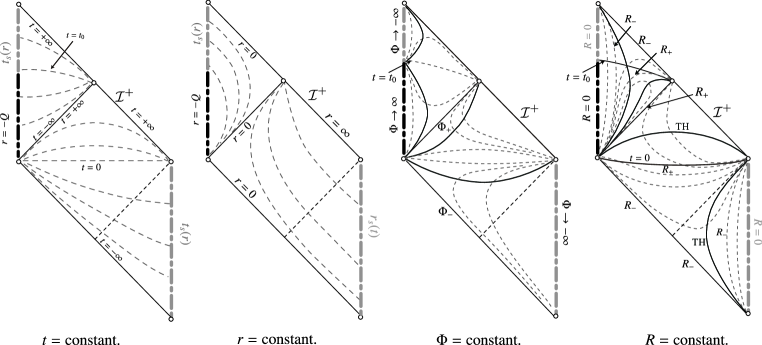
Figure 1: Conformal diagram of a black hole in an expanding universe. The central points $R=0$ describe naked singularities. The lines $t={\rm constant}$ and $r={\rm constant}$ are everywhere spacelike and timelike, respectively, while the $R={\rm constant}$ surfaces change signature across the trapping horizon denoted by TH. The $\Phi={\rm constant}$ surfaces are spacelike at infinity, according with our intuition that a massless scalar field behaves like a stiff matter driving the cosmic expansion. The spacetime can be extended in a non-analytic manner across the null surfaces $R=R_{-}$.

5.3 Generalization to arbitrary power-law expansion

In the previous subsection, a massless scalar field drives a decelerating cosmic expansion $a\propto\bar{t}^{1/3}$. It is then natural to ask what happens when one includes the potential of the scalar field. We shall begin by the $D$-dimensional Einstein-dilaton-${\rm U}(1)^{2}$ system, in which two types of ${\rm U}(1)$-fields couple to the dilaton with different couplings, and the dilaton has a Liouville-type exponential potential [93, 94]. To be specific, the action is described by

$$S= \frac{1}{16\pi G}\int{\rm d}^{D}x\,\sqrt{-g}\,\left[{}^{(D)}R-\left(\nabla\Phi\right)^{2}-V(\Phi)-\sum_{A=S,T}n_{A}e^{\lambda_{A}\Phi}F_{\mu\nu}^{(A)}F^{(A)\mu\nu}\right]\,,$$ (126)

where

$$V(\Phi)=V_{0}\exp(-\alpha\Phi)\,.$$ (127)

Here, $\alpha~{}(\geq 0)$ is a dimensionless constant corresponding to the steepness of the potential. We have introduced degeneracy factors, $n_{A}~{}(\geq 0)$, of two ${\rm U}(1)$ fields for later convenience. These parameters are subjected to the following relations

$$n_{T}+n_{S}=\frac{2(D-2)}{D-3}\,,\qquad\lambda_{T}=\alpha=-\frac{n_{S}}{n_{T}}\lambda_{S}=2\sqrt{\frac{(D-3)n_{S}}{(D-2)n_{T}}}\,.$$ (128)

The constants $n_{T}$ and $n_{S}$ may take natural number only for $D=4,5$, in which case they are related to the number of time-dependent and static branes in eleven-dimensional supergravity [89, 88].

As a natural generalization of the previous metric (110), we obtain a $D$-dimensional spatially-inhomogeneous and time-evolving metric [93, 94],

$${\rm d}s_{D}^{2}=-\Xi^{D-3}{\rm d}t^{2}+\Xi^{-1}\,h_{mn}(x^{p}){\rm d}x^{m}{\rm d}x^{n}\,,$$ (129)

with

$$\Xi:=\left[\left(\frac{t}{t_{0}}+\bar{H}_{T}\right)^{n_{T}}H_{S}^{n_{S}}\right]^{-1/(D-2)}\,,\qquad t_{0}^{2}=\frac{n_{T}(n_{T}-1)}{2V_{0}}\,,$$ (130)

and

$$\Phi =\frac{1}{2}\sqrt{\frac{(D-3)n_{T}n_{S}}{D-2}}\,\ln\left(\frac{H_{T}}{H_{S}}\right)\,,\quad A^{(T)}_{t}=\frac{1}{2H_{T}}\,,\quad A^{(S)}_{t}=\frac{1}{2H_{S}}\,,$$ (131)

where $\bar{H}_{T}(x)$ and $H_{S}(x)$ are harmonics of $(D-1)$-dimensional Ricci-flat base space $h_{mn}{\rm d}x^{m}{\rm d}x^{n}$, and $H_{T}=(t/t_{0})+\bar{H}_{T}$.

When $n_{T}=0$, this is nothing but a static solution derived from BPS intersecting branes (at least for $D=4,5$). For $n_{S}=0$, the potential becomes a positive constant and the higher-dimensional Kastor-Traschen solution [95, 96] is recovered. The $D=4$ and $n_{T}=1$ case reduces to the previous solution with a massless scalar field derived from dynamically intersecting branes. For any positive values of $n_{T}$ and $n_{S}$, this system is shown to obey the weak energy condition.

Consider the $D=4$ case with $\bar{H}_{T}=Q/r$ and $H_{S}=1+Q/r$ for simplicity. Then the solution is specified by three parameters: the Maxwell charge ($Q$), the relative ratio of energy densities of scalar and ${\rm U}(1)$-fields ($\tau=t_{0}/Q$) and the steepness parameter of the potential ($n_{T}$). The asymptotic region of the spacetime is described by the FLRW universe (116) with

$$a(\bar{t})\propto\bar{t}^{p}\,,\qquad p=\frac{n_{T}}{4-n_{T}}\,.$$ (132)

Hence the parameter $n_{T}$ controls the expansion of the background cosmology: the universe decelerates for $n_{T}<2$ and accelerates for $2<n_{T}\leq 4$. The $n_{T}=4$ case corresponds to the exponential expansion caused by a cosmological constant.

Following the argument described in the preceding subsection, we can obtain the conformal diagrams. The spacetime structures fall into nine types (see Table 1 in Ref. [94]). Of our primary interest is the black hole in the accelerating universe, which arises when $n_{T}=4$ (Reissner-Nordström-de Sitter black hole with $M=Q$) or $2<n_{T}<4$ with $\tau\geq n_{T}^{n_{T}/2}(n_{T}-2)^{1-n_{T}/2}/2$. The conformal diagrams for the accelerating cases are shown in Fig 2. The horizon is in general described by the nonextremal (asymptotic) Killing horizon. A novel difference from the decelerating universe is the existence of a cosmological horizon. Figure 1 is the representative for a black hole in the decelerating case ($0<n_{T}<2$).

Figure 2: Conformal diagrams of a black hole in an accelerating universe. The left figure corresponds to $n_{T}=3$, $\tau=3$ (which is the representative for $2<n_{T}<4$ with $\tau\geq n_{T}^{n_{T}/2}(n_{T}-2)^{1-n_{T}/2}/2$, while the right is the $n_{T}=4$ case corresponding to the Reissner-Nordström de Sitter spacetime with $M=Q$. In the accelerating universe, the cosmological horizon (denoted by CH) develops.

5.4 Fake supergravity

A curious property of solutions addressed in the preceding subsections is that the field equations are completely linearized. This fact enables us to superpose the harmonics ad arbitrium to construct multiple solutions in spite of the time-dependence of the metric. This property is reminiscent of supersymmetric solution. But it has been well known that any dynamical phenomena are not compatible with supersymmetry.

Nevertheless, we can in some sense give a supergravity interpretation as follows. It is instrumental to consider the four-dimensional Einstein-Maxwell-$\Lambda$ system, where $\Lambda=-3\ell^{-2}<0$. This is the bosonic sector of $D=4$, $N=2$ gauged supergravity. The inclusion of a negative cosmological constant modifies the super-covariant derivative (3) as

$$\hat{\nabla}_{\mu}\epsilon=\left(\nabla_{\mu}-\frac{i}{\ell}A_{\mu}+\frac{1}{2\ell}\gamma_{\mu}+\frac{i}{4}F_{\nu\rho}\gamma^{\nu\rho}\gamma_{\mu}\right)\epsilon\,.$$ (133)

Since the (inverse of) curvature radius $\ell$ acts as a gauge coupling, this theory is called a gauged supergravity. Such a coupling arises from the R-symmetry. The maximally supersymmetric vacuum is only the anti-de Sitter space [43]. The super-covariant derivative $\hat{\nabla}_{\mu}$ is shown to be hermite if $\ell\in\mathbb{R}$.

Reminding the fact that the bosonic action of $N=2$ gauged supergravity is not charged with respect to the R-symmetry, the Wick rotation $\ell^{-1}\to ih~{}(h\in\mathbb{R})$ of a gauge coupling amounts to changing the sign of the cosmological constant. If there exist charged sectors, the analytic continuation would yield unwanted ghosts [97]. As long as we concentrate on the truncated action composed only of neutral fields, however, there may appear no pathologies (at least classically).

Assuming that the Killing spinor equation $\hat{\nabla}_{\mu}\epsilon=0$ (133) continues to be valid after the Wick rotation $\ell^{-1}\to ih$, the de Sitter spacetime turns out to admit a spinor obeying the 1st-order differential equation. Such a spinor is called a pseudo-Killing spinor and the resulting theory is called a fake supergravity, in distinction from bona fide supergravity.

A time-dependent pseudo-supersymmetric solution in this theory was found by Kastor and Traschen [95, 96], the metric of which takes the exactly the same form as Majumdar-Papapetrou solution (7) up to the inclusion of a linear term in time $H\to ht+\sum_{k}Q_{k}/|\vec{x}-\vec{x}_{k}|$. This is the generalization of Majumdar-Papapetrou solution in the de Sitter background. The Kastor-Traschen solution describes coalescing black holes in the contracting de Sitter universe (or splitting white holes in the expanding de Sitter universe) and inherits some salient characteristics from the Majumdar-Papapetrou solution.

We can show that the $D=5$ solution (129) with a hyper-Kähler base space is in fact a pseudo-supersymmetric solution in minimal fake supergravity coupled to two ${\rm U(1)}$ gauge field and a scalar [101]. It is also possible to extend to theories with arbitrary number of gauge fields and scalars [101, 102] and to include the nonvanishing angular momentum. A notable feature of the spinning solution is that the horizon is rotating, in contrast to the supersymmetric black holes for which the angular velocities of the horizon vanish. This implies that the ergoregion exists, hence the superradiant phenomenon occurs [101]. These rotating solutions generically suffer from closed timelike curves around the singularities. These curves may arise outside the horizon, so that there appear naked time machines.

Recently, there has been a progress in the classifications of pseudo-supersymmetric solutions [103] and their near-horizon geometries [104]. It is shown that the general rotating solution admits a torsion on the hyper-Kähler base space. It is interesting to see if a black hole solution with nonvanishing torsion exists.

6 Concluding remarks and outlooks

Based on supergravity theories, which may arise from string/M-theory in the low energy field theory limit, we have discussed supersymmetric black holes and their relatives. We have discussed two approaches: one is a classification method of supersymmetric solutions in five dimensions, finding general black hole solutions and their relatives, and the other is how to construct four or five dimensional black hole solutions by compactifying intersecting brane solutions in ten or eleven dimensions. These complementary strategies have unveiled very interesting solutions describing various kinds of black objects. Though, the full landscape of black hole solutions, which is expected to be very wealthy, have been yet uncovered. This field of study leaves much room for discussion.

For the supersymmetric black objects in supergravities, prime examples of unsettled open problems are the followings:

• It seems reasonable to anticipate that black rings exist in AdS, but at present no exact solution is available. The most efficient way toward this is to impose BPS condition as described in § 3.2. It is demonstrated, however, that the black ring in minimal supergravity suffers from conical singularities if it has ${\rm U}(1)^{2}$ spatial symmetries [105]. It is likely that the black ring may be invariant under the isometry $V^{M}=i\bar{\epsilon}\gamma^{M}\epsilon$, but may not be invariant under the usual time translation at infinity. Such a less symmetric black object is not excluded by the rigidity theorem [106], and if discovered it might trigger a rapid increase in our knowledge about higher dimensional black holes.

• Asymptotically flat, supersymmetric black holes in $D\geq 6$ have not been found yet. In the static case, the intersecting branes fail to produce supersymmetric black holes in $D\geq 6$ with nonvanishing horizon [see Eq. (95)]. Furthermore, the solution-generating technique is less powerful in $D\geq 6$ dimensions. According to the classification of Ref. [41] for the minimal supergravity in six dimensions, the supersymmetric Killing field is null everywhere, which cannot be a null generator of a black hole horizon. If we impose additional supersymmetries, the supersymmetric Killing field may be combined to give a desired one, and things may be tractable.

In the latter case, we find the spacetime solutions from simple time-dependent brane solutions, which describe black holes in the expanding universe with arbitrary power-law expansion. Some remaining questions and future works are listed as follows:

• Some black hole solutions have a link to time-dependent intersecting brane systems in eleven-dimensional supergravity model. We have not found, however, any intersecting brane solutions in higher dimensions, which reduce to the effective action involving a Liouville-type potential. The exponential potential is responsible for the expanding universe with power-law expansion. It is interesting to find them and see whether any fundamental or deep reason exists.

• Can we find more realistic black hole solutions? Although it was straightforward to include rotation in five dimensions [101], the solution suffers from causal violation, hence physically unacceptable. A more fundamental question from the general relativistic point of view is whether neutral black holes exist in the expanding universe. When the time-dependence is incorporated for non (pseudo-)supersymmetric solution, ambient matter will accrete into a black hole and the radius of a black hole increases in time. These dynamical processes are desirable in real world, but the construction of exact solution is a formidable task since we cannot resort to the 1st-order BPS equations. The construction of these truly dynamical black holes is very hard under the energy condition.

• Can we formulate black hole thermodynamics in the time-dependent spacetimes? In a particular case where the horizon is described by the (asymptotic) Killing field, this is promising since the “intensive parameters” such as surface gravity, angular velocity of the horizon can be defined (apart from the normalization). The most difficult issue is how to define the mass of the hole. The present time-dependent solution may provide us a good tool to analyze this question in more detail. The black hole evaporation in an expanding universe is relevant for the observational restriction of primordial black holes. It is also a challenging task to account for the entropy from the statistical point of view. It is interesting to investigate if the “attractor mechanism” [107] continues to hold in a time-dependent case.

• The black hole collision in the contracting universe may be handled just as the Kastor-Traschen spacetime [95]. This is an outstanding privilege since we are able to access it by exact solution. The numerical analysis of horizon formation has been reported in Ref. [108]. Similarly, it is expected that we can discuss the brane collision with multi time-dependent branes, which is a generalization of the solution in Ref. [86]. It may be of interest to examine if the quantitative picture of coalescence changes depending on the acceleration or the deceleration of the universe.

• Although we have discussed lowest order effective theories, the higher curvature terms will come to be unignorable as the energy goes up. It has been uncovered that higher curvature corrections drastically change the singularity structure of black holes (see, e.g., papers [109] and references therein). Can we obtain exact time-dependent solutions in such theories? A more moderate question is: how to fit the higher curvature terms into the framework of (pseudo) supergravity?

In order to promote a better understanding about higher dimensional (pseudo) supersymmetric black holes and their applications to real world, it is of crucial importance to resolve these outstanding problems.

References

- [1] See other articles in this supplement.
- [2] R. Emparan and H. S. Reall, Phys. Rev. Lett. 88 (2002), 101101 [arXiv:hep-th/0110260].
- [3] A. A. Pomeransky and R. A. Sen’kov, arXiv:hep-th/0612005.
- [4] R. C. Myers and M. J. Perry, Annals Phys. 172 (1986), 304.
- [5] R. Gregory and R. Laflamme, Phys. Rev. Lett. 70 (1993), 2837 [arXiv:hep-th/9301052]; Nucl. Phys. B 428 (1994), 399 [arXiv:hep-th/9404071].
- [6] G. T. Horowitz and K. Maeda, Phys. Rev. Lett. 87 (2001), 131301; M. W. Choptuik, et al., Phys. Rev. D 68 (2003), 044001.
- [7] B. Kol, Phys. Rept. 422 (2006), 119; T. Harmark, V. Niarchos and N.A. Obers, Class. Quant. Grav. 24 (2007), R1.
- [8] T. Harmark, Phys. Rev. D69 (2004), 104015; H. Kudoh and T. Wiseman, Prog. Theor. Phys. 111 (2004), 475; H. Kudoh and T. Wiseman, Phys. Rev. Lett. 94 (2005), 161102; S.S. Gubser, Class. Quant. Grav. 19 (2002), 4825; T. Wiseman, Class. Quant. Grav. 20 (2003), 1137; E. Sorkin, Phys. Rev. D74 (2006), 104027; E. Sorkin, Phys. Rev. Lett. 93 (2004), 031601; H. Kudoh and U. Miyamoto, Class. Quant. Grav. 22 (2005), 3853; U. Miyamoto, K. Maeda, Phys. Lett. B664 (2008), 103 [arXiv:0803.3037 [hep-th]].
- [9] R. Emparan, T. Harmark, V. Niarchos et al., JHEP 0710 (2007), 110. [arXiv:0708.2181 [hep-th]].
- [10] E. Witten and D. I. Olive, Phys. Lett. B 78 (1978), 97.
- [11] J. D. Bekenstein, Phys. Rev. D7 (1973), 2333; Phys. Rev. D 12 (1975), 3077.
- [12] S. W. Hawking, Commun. Math. Phys. 43 (1975), 199.
- [13] A. Strominger and C. Vafa, Phys. Lett. B 379 (1996), 99 [arXiv:hep-th/9601029].
- [14] J. M. Bardeen, B. Carter, S. W. Hawking, Commun. Math. Phys. 31 (1973), 161.
- [15] J. M. Maldacena, arXiv:hep-th/9607235.
- [16] J. M. Maldacena, Adv. Theor. Math. Phys. 2 (1998), 231 [Int. J. Theor. Phys. 38 (1999), 1113] [arXiv:hep-th/9711200]; O. Aharony, S. S. Gubser, J. M. Maldacena et al., Phys. Rept. 323 (2000), 183. [hep-th/9905111].
- [17] R. Arnowitt, S. Deser and C. W. Misner, Gravitation, An Introduction to Current Research, edited by L. Witten, (Wiley, New York, 1962).
- [18] R. Schon and S. T. Yau, Commun. Math. Phys. 65 (1979), 45; R. Schon and S. T. Yau, Commun. Math. Phys. 79 (1981), 231.
- [19] G. W. Gibbons, K. Maeda and U. Miyamoto, Class. Quant. Grav. 26 (2009), 185008 [arXiv:0906.0264 [hep-th]].
- [20] E. Witten, Commun. Math. Phys. 80 (1981), 381.
- [21] J. A. Nester, Phys. Lett. A 83 (1981), 241.
- [22] G. W. Gibbons and C. M. Hull, Phys. Lett. B 109 (1982), 190.
- [23] G. T. Horowitz and A. Strominger, Phys. Rev. D 27 (1983), 2793; C. M. Hull, Commun. Math. Phys. 90 (1983), 545.
- [24] M. Nozawa, arXiv:1011.0261 [hep-th].
- [25] G. W. Gibbons, G. T. Horowitz, P. K. Townsend, Class. Quant. Grav. 12 (1995) 297-318. [hep-th/9410073].
- [26] S. D. Majumdar, Phys. Rev. 72 (1947), 390; A. Papaetrou, Proc. Roy. Irish Acad. (Sect. A) A 51 (1947), 191.
- [27] J. B. Hartle and S. W. Hawking, Commun. Math. Phys. 26 (1972), 87.
- [28] Z. Perjes, Phys. Rev. Lett. 27 (1971), 1668; W. Israel and G. A. Wilson, J. Math. Phys. 13 (1972), 865.
- [29] H. Stephani, D. Kramer, M. A. H. MacCallum, C. Hoenselaers and E. Herlt, “Exact solutions of Einstein’s field equations,” Cambridge, UK: Univ. Pr. (2003).
- [30] R. Penrose, Riv. Nuovo Cim. 1 (1969), 252.
- [31] B. Carter, Black Hole Equilibrium States in Black Holes, edited by C. DeWitt and J. DeWitt (Gordon and Breach, New York, 1973).
- [32] J. Kowalski-Glikman, Phys. Lett. B 150 (1985), 125.
- [33] K. P. Tod, Phys. Lett. B 121 (1983), 241.
- [34] P. T. Chrusciel, H. S. Reall, P. Tod, Class. Quant. Grav. 23 (2006), 2519. [gr-qc/0512116].
- [35] T. Ortin, JHEP 0805 (2008), 034 [arXiv:0802.1799 [hep-th]]; P. Meessen and T. Ortin, Nucl. Phys. B 749 (2006), 291 [arXiv:hep-th/0603099].
- [36] K. P. Tod, Class. Quant. Grav. 12 (1995), 1801.
- [37] A. Sen, Phys. Rev. Lett. 69 (1992), 1006 [arXiv:hep-th/9204046].
- [38] J. P. Gauntlett, J. B. Gutowski, C. M. Hull, S. Pakis and H. S. Reall, Class. Quant. Grav. 20 (2003), 4587 [arXiv:hep-th/0209114].
- [39] J. P. Gauntlett, N. Kim, D. Martelli, D. Waldram, JHEP 0111 (2001), 018. [hep-th/0110034]; J. P. Gauntlett, D. Martelli, S. Pakis, D. Waldram, Commun. Math. Phys. 247 (2004), 421. [hep-th/0205050].
- [40] J. P. Gauntlett and J. B. Gutowski, Phys. Rev. D 68 (2003), 105009 [Erratum-ibid. D 70 (2004), 089901] [arXiv:hep-th/0304064].
- [41] J. B. Gutowski, D. Martelli and H. S. Reall, Class. Quant. Grav. 20 (2003), 5049 [arXiv:hep-th/0306235].
- [42] J. B. Gutowski, W. Sabra, JHEP 0510 (2005), 039. [hep-th/0505185]; J. B. Gutowski, W. A. Sabra, JHEP 0712 (2007), 025. [arXiv:0706.3147 [hep-th]]; J. Grover, J. B. Gutowski, W. Sabra, JHEP 0810 (2008), 103. [arXiv:0802.0231 [hep-th]].
- [43] M. M. Caldarelli and D. Klemm, JHEP 0309 (2003), 019 [arXiv:hep-th/0307022]; S. L. Cacciatori, M. M. Caldarelli, D. Klemm, D. S. Mansi, JHEP 0407 (2004), 061 [hep-th/0406238]; S. L. Cacciatori, M. M. Caldarelli, D. Klemm, D. S. Mansi, D. Roest, JHEP 0707 (2007), 046. [arXiv:0704.0247 [hep-th]]; S. L. Cacciatori, D. Klemm, D. S. Mansi, E. Zorzan, JHEP 0805, 097 (2008). [arXiv:0804.0009 [hep-th]].
- [44] J. B. Gutowski and H. S. Reall, JHEP 0404 (2004), 048 [arXiv:hep-th/0401129].
- [45] J. P. Gauntlett and S. Pakis, JHEP 0304 (2003), 039 [arXiv:hep-th/0212008]; J. P. Gauntlett, J. B. Gutowski and S. Pakis, JHEP 0312 (2003), 049 [arXiv:hep-th/0311112].
- [46] J. Bellorin, P. Meessen and T. Ortin, JHEP 0701 (2007), 020 [arXiv:hep-th/0610196]; J. Bellorin and T. Ortin, JHEP 0708 (2007), 096 [arXiv:0705.2567 [hep-th]];
- [47] J. M. Figueroa-O’Farrill and G. Papadopoulos, JHEP 0303 (2003), 048 [arXiv:hep-th/0211089].
- [48] J. P. Gauntlett, D. Martelli, J. Sparks and D. Waldram, arXiv:hep-th/0411194.
- [49] J. Gillard, U. Gran and G. Papadopoulos, Class. Quant. Grav. 22 (2005), 1033 [arXiv:hep-th/0410155]; U. Gran, J. Gutowski and G. Papadopoulos, Class. Quant. Grav. 22 (2005), 2453 [arXiv:hep-th/0501177]; U. Gran, G. Papadopoulos, D. Roest, Class. Quant. Grav. 22 (2005), 2701 [hep-th/0503046]; U. Gran, J. Gutowski, G. Papadopoulos, Class. Quant. Grav. 23 (2006) 143-206 [hep-th/0505074]; U. Gran, J. Gutowski, G. Papadopoulos, D. Roest, Class. Quant. Grav. 23 (2006) 1617-1678. [hep-th/0507087]. U. Gran, P. Lohrmann and G. Papadopoulos, JHEP 0602 (2006), 063 [arXiv:hep-th/0510176].
- [50] S. Kobayashi and K. Nomizu, Foundations of Differential Geometry, Vol II, (Wiley Classics Library, 1996).
- [51] G. W. Gibbons, D. Kastor, L. A. J. London, P. K. Townsend and J. H. Traschen, Nucl. Phys. B 416 (1994), 850 [arXiv:hep-th/9310118].
- [52] J. C. Breckenridge, R. C. Myers, A. W. Peet and C. Vafa, Phys. Lett. B 391 (1997), 93 [arXiv:hep-th/9602065].
- [53] G. T. Horowitz and A. Sen, Phys. Rev. D 53 (1996), 808 [arXiv:hep-th/9509108].
- [54] G. W. Gibbons and C. A. R. Herdeiro, Class. Quant. Grav. 16 (1999), 3619 [arXiv:hep-th/9906098].
- [55] J. P. Gauntlett, R. C. Myers and P. K. Townsend, Class. Quant. Grav. 16 (1999), 1 [arXiv:hep-th/9810204].
- [56] D. Sudarsky and R. M. Wald, Phys. Rev. D 46 (1992), 1453; D. Sudarsky and R. M. Wald, Phys. Rev. D 47 (1993), 5209 [arXiv:gr-qc/9305023].
- [57] H. K. Kunduri, J. Lucietti and H. S. Reall, Class. Quant. Grav. 24 (2007), 4169 [arXiv:0705.4214 [hep-th]].
- [58] H. S. Reall, Phys. Rev. D 68 (2003), 024024 [Erratum-ibid. D 70 (2004), 089902] [arXiv:hep-th/0211290].
- [59] H. Elvang, R. Emparan, D. Mateos and H. S. Reall, Phys. Rev. Lett. 93 (2004), 211302 [arXiv:hep-th/0407065].
- [60] H. Elvang, R. Emparan, D. Mateos and H. S. Reall, Phys. Rev. D 71 (2005), 024033 [arXiv:hep-th/0408120].
- [61] M. Nozawa and K. Maeda, Phys. Rev. D 71 (2005), 084028 [arXiv:hep-th/0502166].
- [62] I. Bena, Phys. Rev. D 70 (2004), 105018 [arXiv:hep-th/0404073].
- [63] J. P. Gauntlett and J. B. Gutowski, Phys. Rev. D 71 (2005), 045002 [arXiv:hep-th/0408122].
- [64] G. W. Gibbons and S. W. Hawking, Phys. Lett. B 78 (1978), 430.
- [65] H. Elvang, R. Emparan, D. Mateos and H.S. Reall, JHEP 0508 (2005), 042; I. Bena, P. Kraus and N.P. Warner, Phys. Rev. D 72 (2005), 084019.
- [66] R. C. Myers, Phys. Rev. D 35 (1987), 455.
- [67] K. Maeda, N. Ohta, M. Tanabe, Phys. Rev. D 74 (2006), 104002 [hep-th/0607084].
- [68] I. Bena and N. P. Warner, Adv. Theor. Math. Phys. 9 (2005), 667 [arXiv:hep-th/0408106].
- [69] H. Elvang, P. Figueras, JHEP 0705 (2007), 050. [hep-th/0701035].
- [70] M. Cvetic, M. J. Duff, P. Hoxha et al., Nucl. Phys. B558 (1999), 96. [hep-th/9903214].
- [71] M. Cvetic, P. Gao and J. Simon, Phys. Rev. D 72 (2005), 021701 [arXiv:hep-th/0504136].
- [72] S. W. Hawking, C. J. Hunter and M. Taylor, Phys. Rev. D 59 (1999), 064005 [arXiv:hep-th/9811056]; G. W. Gibbons, H. Lu, D. N. Page and C. N. Pope, J. Geom. Phys. 53 (2005), 49 [arXiv:hep-th/0404008].
- [73] A. Ashtekar, S. Das, Class. Quant. Grav. 17 (2000), L17-L30. [hep-th/9911230]; S. Hollands, A. Ishibashi and D. Marolf, Class. Quant. Grav. 22 (2005), 2881 [arXiv:hep-th/0503045].
- [74] G. W. Gibbons, M. J. Perry, C. N. Pope, Class. Quant. Grav. 22 (2005), 1503 [hep-th/0408217].
- [75] J. B. Gutowski and H. S. Reall, JHEP 0402 (2004), 006 [arXiv:hep-th/0401042].
- [76] G. W. Gibbons, C. M. Hull, N. P. Warner, Nucl. Phys. B218 (1983), 173.
- [77] O. Coussaert and M. Henneaux, Phys. Rev. Lett. 72 (1994), 183 [arXiv:hep-th/9310194]; V. A. Kostelecky and M. J. Perry, Phys. Lett. B 371 (1996), 191 [arXiv:hep-th/9512222]; M. M. Caldarelli, D. Klemm, Nucl. Phys. B545 (1999), 434. [hep-th/9808097].
- [78] P. T. Chrusciel, D. Maerten and P. Tod, JHEP 0611 (2006), 084 [arXiv:gr-qc/0606064].
- [79] H. K. Kunduri, J. Lucietti and H. S. Reall, JHEP 0604 (2006), 036 [arXiv:hep-th/0601156].
- [80] P. Candelas, G. T. Horowitz, A. Strominger and E. Witten, Nucl. Phys. B 258 (1985), 46; G. Papadopoulos and P. K. Townsend, Phys. Lett. B 357 (1995), 300 [arXiv:hep-th/9506150].
- [81] J. P. Gauntlett, [hep-th/9705011].
- [82] M. Cvetic, D. Youm, Nucl. Phys. B499 (1997), 253. [hep-th/9612229]; J. P. Gauntlett, R. C. Myers, P. K. Townsend, Phys. Rev. D59 (1999), 025001 [hep-th/9809065].
- [83] K. Maeda and M. Tanabe, Nucl. Phys. B738 (2006), 184.
- [84] A. A. Tseytlin, Nucl. Phys. B 475 (1996), 149 [arXiv:hep-th/9604035]; A. A. Tseytlin, Nucl. Phys. B487 (1997), 141 [hep-th/9609212]; R. Argurio, F. Englert, L. Houart, Phys. Lett. B398 (1997), 61 [hep-th/9701042]; N. Ohta, Phys. Lett. B 403 (1997) 218 [arXiv:hep-th/9702164].
- [85] J. Khoury, B. A. Ovrut, P. J. Steinhardt and N. Turok, Phys. Rev. D 64 (2001), 123522 [arXiv:hep-th/0103239].
- [86] G. W. Gibbons, H. Lu and C. N. Pope, Phys. Rev. Lett. 94 (2005), 131602 [arXiv:hep-th/0501117].
- [87] W. Chen, Z. W. Chong, G. W. Gibbons, H. Lu and C. N. Pope, Nucl. Phys. B 732 (2006), 118 [arXiv:hep-th/0502077].
- [88] K. Maeda, N. Ohta and K. Uzawa, JHEP 0906 (2009), 051 [arXiv:0903.5483 [hep-th]].
- [89] K. Maeda and M. Nozawa, Phys. Rev. D 81 (2010), 044017 [arXiv:0912.2811 [hep-th]].
- [90] S. W. Hawking and G. F. R. Ellis, The large scale structure of space-time (Cambridge: Cambridge University Press, 1973).
- [91] S. A. Hayward, Phys. Rev. D 49 (1994), 6467.
- [92] M. Nozawa and H. Maeda, Class. Quant. Grav. 25 (2008), 055009 [arXiv:0710.2709 [gr-qc]].
- [93] G. W. Gibbons and K. Maeda, Phys. Rev. Lett. 104 (2010), 131101 [arXiv:0912.2809 [gr-qc]].
- [94] K. Maeda and M. Nozawa, Phys. Rev. D 81 (2010), 124038 [arXiv:1003.2849 [gr-qc]].
- [95] D. Kastor and J. Traschen, Phys. Rev. D 47 (1993), 5370 [arXiv: hep-th/9212035].
- [96] L. A. J. London, Nucl. Phys. B 434 (1995), 709.
- [97] M. Cvetic, G. W. Gibbons and C. N. Pope, Nucl. Phys. B 708 (2005), 381 [arXiv:hep-th/0401151].
- [98] D. Z. Freedman, C. Nunez, M. Schnabl and K. Skenderis, Phys. Rev. D 69 (2004), 104027 [arXiv:hep-th/0312055].
- [99] K. Skenderis and P. K. Townsend, Phys. Rev. Lett. 96 (2006), 191301 [arXiv:hep-th/0602260]. K. Skenderis and P. K. Townsend, Phys. Rev. D 74 (2006), 125008 [arXiv:hep-th/0609056]; P. K. Townsend, Class. Quant. Grav. 25 (2008), 045017 [arXiv:0710.5178 [hep-th]].
- [100] T. Shiromizu, D. Ida and T. Torii, JHEP 0111 (2001), 010 [arXiv:hep-th/0109057]; D. Kastor and J. H. Traschen, Class. Quant. Grav. 19 (2002), 5901 [arXiv:hep-th/0206105].
- [101] M. Nozawa and K. Maeda, Phys. Rev. D 83 (2011), 024018 [arXiv:1009.3688 [hep-th]].
- [102] K. Behrndt and M. Cvetic, Class. Quant. Grav. 20 (2003), 4177 [arXiv:hep-th/0303266]; D. Klemm and W. A. Sabra, JHEP 0102 (2001), 031 [arXiv:hep-th/0011016]; D. Klemm, W. A. Sabra, Phys. Lett. B503 (2001), 147 [hep-th/0010200]. J. T. Liu, W. A. Sabra, Phys. Lett. B498 (2001), 123 [hep-th/0010025].
- [103] J. Grover, J. B. Gutowski, C. A. R. Herdeiro and W. Sabra, Nucl. Phys. B 809 (2009), 406 [arXiv:0806.2626 [hep-th]]; J. B. Gutowski and W. A. Sabra, arXiv:1009.4453 [hep-th]; J. Grover, J. B. Gutowski, C. A. R. Herdeiro, P. Meessen, A. Palomo-Lozano and W. A. Sabra, JHEP 0907 (2009), 069 [arXiv:0905.3047 [hep-th]].
- [104] J. Grover, J. Gutowski, JHEP 1004 (2010), 009. [arXiv:1001.2460 [hep-th]]; J. B. Gutowski, W. A. Sabra, [arXiv:1012.2120 [hep-th]].
- [105] H. K. Kunduri, J. Lucietti, H. S. Reall, JHEP 0702 (2007), 026 [hep-th/0611351].
- [106] S. Hollands, A. Ishibashi, R. M. Wald, Commun. Math. Phys. 271 (2007), 699 [gr-qc/0605106]; Commun. Math. Phys. 291 (2009), 443 [arXiv:0809.2659 [gr-qc]].
- [107] A. Sen, JHEP 0509 (2005), 038 [hep-th/0506177].
- [108] K. -I. Nakao, T. Shiromizu, S. A. Hayward, Phys. Rev. D52 (1995), 796.
- [109] T. Torii, H. Yajima, K. Maeda, Phys. Rev. D 55 (1997), 739 [arXiv:gr-qc/9606034]; T. Torii and H. Maeda, Phys. Rev. D 71 (2005), 124002 [arXiv:hep-th/0504127]; Z. K. Guo, N. Ohta and T. Torii, Prog. Theor. Phys. 120 (2008), 581 [arXiv:0806.2481 [gr-qc]]; Prog. Theor. Phys. 121, 253-273 (2009). [arXiv:0811.3068 [gr-qc]]; N. Ohta, T. Torii, Prog. Theor. Phys. 121, 959-981 (2009). [arXiv:0902.4072 [hep-th]]; Prog. Theor. Phys. 122, 1477-1500 (2009). [arXiv:0908.3918 [hep-th]]; Prog. Theor. Phys. 124, 207-225 (2010). [arXiv:1004.2779 [hep-th]]. K. Maeda, N. Ohta and Y. Sasagawa, Phys. Rev. D 80 (2009), 104032 [arXiv:0908.4151 [hep-th]]; Phys. Rev. D83 (2011), 044051 [arXiv:1012.0568 [hep-th]].