Collinear to Anti-collinear Quantum Phase Transition by Vacancies

Abstract

We study static vacancies in the collinear magnetic phase of a frustrated Heisenberg $J_{1}$-$J_{2}$ model. It is found that vacancies can rapidly suppress the collinear antiferromagnetic state (CAFM) and generate a new magnetic phase, an anti-collinear magnetic phase (A-CAFM), due to magnetic frustration. We investigate the quantum phase transition between these two states by studying a variety of vacancy superlattices. We argue that the anti-collinear magnetic phase can exist in iron-based superconductors in the absence of any preceding structural transitions and an observation of this novel phase will unambiguously resolve the relation between the magnetic and structural transitions in these materials.

There are several reasons for studying static vacancy problems on frustrated magnetic systems. First of all, there has been convincing experimental evidence which supports the magnetism in iron-based high temperature superconductors ($Fe$-HTSC) can be understood by an effective frustrated magnetic model ($J_{1}$-$J_{2}$-$J_{z}$ model) Fang2008d ; Si2008 ; Xu2008a ; Yildirim2008 which simultaneously captures the collinear antiferromagnetic state and the tetragonal to orthohombic structural transition observed in neutron-scattering experiments Cruz2008 . The new superconductors are very flexible in substituting $Fe$ by other transition metal atoms, such as $Mn$, $Zn$, $Co$ and $Ni$. The static-vacancy problem in the $J_{1}$-$J_{2}$-$J_{z}$ model is, then, an important low energy effective model for non-magnetic $Zn$-doped $Fe$-HTSC Cheng2010 . Moreover, the recently discovered 122 iron-chalcogenide, $(K,Cs)Fe_{2-x}Se_{2}$ Guo2010 ; Fang2010 ; Liu2011 , carries intrinsic iron vacancies, which can even form superlattice vacancy structures Bao2011a ; Bacsa2011 ; Pomjakushin2011b ; WangZ2011 ; Zavalij2011 ; ZhangAM2011 . Thus, the solution of the static-vacancy problem can be directly tested experimentally and contributes to a fundamental understanding regarding the role of magnetism in superconductivity as well as the coupling between lattice and magnetism. Second, with various frustrated magnetic materials being discovered in the past decade, many novel physics and new states of matter have been proposed. However, experimentally, it has often been difficult to identify features associated to novel physics, for example, spin liquid state Shimizu2003 ; Lee2005 . Static vacancies can either enhance or decrease the degree of frustration and can behave rather differently in different state of matters. Therefore, static vacancies can contribute to a new understanding of frustrated magnetic physics and provide unique features that can be probed experimentally. Finally, even in a standard quantum Heisenberg antiferromagnetic model, it has been shown that quantum fluctuations can also be dramatically modified around static vacancies Bulut1989 ; Chen2010 . Studying static vacancies in frustrated quantum magnetic systems can also provide a deeper understanding of the interplay between quantum fluctuations and geometric frustration.

In this Letter, we study the static vacancy problem in the $J_{1}$-$J_{2}$ antiferromagntic Heisenberg model. We employ a linear spin-wave (LSW) theory Bulut1989 to understand properties of a single static vacancy and static vacancy superlattices. We show, depending on the frustrated coupling, quantum fluctuations can be either reduced or enhanced on neighbors of an isolated vacancy. More importantly, by calculating the exact ground-state properties of a variety of static vacancy lattices, we predict that sufficient static vacancies can cause a quantum phase transition between the collinear magnetic phase and an anti-collinear magnetic phase before a spin glassy phase without a spatial long-range magnetic order is formed.

Without vacancies, the $J_{1}$-$J_{2}$ model is given by

$$H_{0}=J_{1}\sum_{<ij>_{NN}}\hat{S}_{i}\cdot\hat{S}_{j}+J_{2}\sum_{<ij>_{NNN}}\hat{S}_{i}\cdot\hat{S}_{j},$$ (1)

where $<ij>_{NN}$ and $<ij>_{NNN}$ denote bonds formed by two nearest neighbor sites and two next nearest neighbor sites respectively. For a classical $J_{1}$-$J_{2}$ model with $J_{1}<2J_{2}$, the ground state can be viewed as two decoupled antiferromagnetically (AFM) ordered states on the A and B sublattices as shown in Fig.1. Including quantum fluctuations, the relative angle between the two antiferromagnetic orders on the A and B sublattices is locked and the quantum model has a CAFM ground state with an ordering wave vector at $Q=(0,\pi)$ or $Q^{\prime}=(\pi,0)$. The CAFM state is driven by the frustrated coupling $J_{1}$. The energy of quantum fluctuations can be calculated using the standard LSW theory. Without losing generality, we take the AFM order in the A sublattice as $S^{z}_{A}\neq 0$ and the AFM order in the B sublattice rotates by $\theta$ around y-axis relative to the one in the A sublattice. Namely,

$$\left(\begin{array}[]{c}S^{B}_{x}\\ S^{B}_{y}\\ S^{B}_{z}\end{array}\right)=\left(\begin{array}[]{ccc}{\rm cos}\theta&&{\rm sin}\theta\\ &1&\\ -{\rm sin}\theta&&{\rm cos}\theta\end{array}\right)\left(\begin{array}[]{c}S^{A}_{x}\\ S^{A}_{y}\\ S^{A}_{z}\end{array}\right),$$ (11)

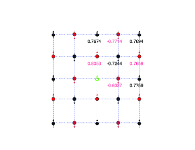
Figure 1: (color online) The sketch of the CAFM state in the $J_{1}-J_{2}$ model where the two sublattices A and B are colored by black and red respectively and a single vacancy site is at the center. The numbers labels the magnetic order parameter $<S_{z}(i)>$ at each site in the CAFM state in the presence of a single vacancy for the parameters $J_{1}=J_{2}$ and $S=1$ (without the vacancy, the magnetic order parameter is $|<S_{z}(i)>|=0.7817$).

In the LSW approximation, Eq.(1) reduces to

$$H_{0} = \sum_{k}\omega_{k}b^{\dagger}_{k}b_{k}+\frac{\nu_{k}}{2}(b_{-k}b_{k}+{\rm h.c.})-4NJ_{2}S^{2},$$ (12)

where, $\omega_{k}=S[J_{1}{\rm cos}\theta({\rm cos}k_{x}-{\rm cos}k_{y})+J_{1}({\rm cos}k_{x}+{\rm cos}k_{y})+4J_{2}]$, $\nu_{k}=S[J_{1}{\rm cos}\theta({\rm cos}k_{x}-{\rm cos}k_{y})-J_{1}({\rm cos}k_{x}+{\rm cos}k_{y})-4J_{2}{\rm cos}k_{x}{\rm cos}k_{y}]$, and $b$ ($b^{+}$) are magnon annihilation (creation) operators. Using the Bogliubov transformation, $\hat{b}_{k}={\rm cosh}\psi_{k}\alpha_{k}+{\rm sinh}\psi_{k}\alpha^{\dagger}_{-k},$ Eq.(12) can be diagonalized as

$$H_{0}=\sum_{k}\tilde{\omega}_{k}\alpha^{\dagger}_{k}\alpha_{k}+N\epsilon_{0}-4NJ_{2}S(S+1),$$ (13)

where, $\tilde{\omega}_{k}=\sqrt{\omega^{2}_{k}-\nu^{2}_{k}},$

${\rm cosh}^{2}\psi=\frac{1}{2}\Big{[}\frac{\omega_{k}}{\sqrt{\omega^{2}_{k}-\nu^{2}_{k}}}+1\Big{]}$, ${\rm sinh}^{2}\psi=\frac{1}{2}\Big{[}\frac{\omega_{k}}{\sqrt{\omega^{2}_{k}-\nu^{2}_{k}}}-1\Big{]}$, and

$$\epsilon_{0}=\frac{1}{N}\sum_{k}\frac{1}{2}\sqrt{\omega^{2}_{k}-\nu^{2}_{k}}=c-a_{0}\frac{J^{2}_{1}S}{J_{2}}{\rm cos}^{2}\theta,$$ (14)

where $c$ is independent of $\theta$ and $a_{0}\simeq 0.033$. $\epsilon_{0}$ describes the well-known “order by disorder mechanism” and has a minimum at $\theta=0,\pi$, favoring a CAFM order Henley1989 ; Chandra1990 ; Fang2008d .

For a single vacancy at the origin of the A-sublattice, the total Hamiltonian can be written as $H=H_{0}-V$ with $V=J_{1}\sum_{i_{NN}}\hat{S}_{0}\cdot\hat{S}^{B}_{i}+J_{2}\sum_{j_{NNN}}\hat{S}_{0}\cdot\hat{S}^{A}_{j}.$ In the LSW approximation, the Hamiltonian becomes

$$H=\sum_{k}\tilde{\omega}_{k}\alpha^{\dagger}_{k}\alpha_{k}-\frac{1}{N}\sum_{k}C_{k}(\alpha_{k}+\alpha^{\dagger}_{k})+(N-1)\epsilon_{0}-\frac{1}{N^{2}}\sum_{\vec{k},\vec{q}}\left[\widetilde{A}_{k,q}\alpha^{\dagger}_{k+q}\alpha_{k}+\frac{B_{k,q}}{2}(\alpha^{\dagger}_{-k+q}\alpha^{\dagger}_{k}+\alpha_{-k+q}\alpha_{k})\right].$$ (15)

where $\widetilde{A}_{k,q}=A_{k,q}{\rm cosh}(\psi_{k+q}+\psi_{k})+\nu_{k}{\rm sinh}(\psi_{k+q}+\psi_{k})$, $B_{k,q}=A_{k,q}{\rm sinh}(\psi_{k+q}+\psi_{k})+\nu_{k}{\rm cosh}(\psi_{k+q}+\psi_{k})$, and $C_{k}=\mu_{k}({\rm cosh}\psi_{k}+{\rm sinh}\psi_{k})$ with $\mu_{k}=-2SJ_{1}\sqrt{S/2}{\rm sin}\theta({\rm cos}k_{x}-{\rm cos}k_{y})$. Up to the first order of $J_{1}^{2}/J_{2}$, the total ground state energy in the presence of a single vacancy is $E_{0}=-4(N-1)J_{2}S(S+1)+(N-1)\epsilon_{0}+\epsilon_{v}$, where

$$\epsilon_{v}=-\frac{1}{N}\sum_{k}\frac{C^{2}_{k}}{\sqrt{\omega^{2}_{k}-\nu^{2}_{k}}}=-a_{1}\frac{J_{1}^{2}S^{2}}{J_{2}}{\rm sin}^{2}\theta,$$ (16)

where $a_{1}\simeq 0.36$. $\epsilon_{v}$ has a minimum at $\theta=\pm\pi/2$ and does not favor a CAFM state. The physics behind the energy $\epsilon_{v}$ can be argued as follows. In the CAFM state, creating a vacancy at one sublattice is similar to applying an external magnetic field along magnetic ordered direction on the four neighbor sites of the vacancy in the other sublattice. Since the spins of the four neighbor sites are AFM, the presence of such a field would favor the AFM order in the four neighbor sites to be perpendicular to the external magnetic field direction. $\epsilon_{0}$ and $\epsilon_{v}$ have different dependence on the spin $S$. The competition between these two energies can lead to a new phase transition.

Considering the model with a small density of vacancies, $\rho$, in the first order approximation and up to a constant, we can approximate the energy density of the model as a function of $\theta$ to be

$$\epsilon(\theta,\rho)=(1-\rho)\epsilon_{0}(\theta)+\rho\epsilon_{v}(\theta).$$ (17)

The energy density favors the CAFM state($\theta=0,\pi$) if $\rho<\rho_{c}$ and an A-CAFM state ($\theta=\pm\pi/2$) if $\rho>\rho_{c}$ where the critical vacancy density is given by

$$\rho_{c}=\frac{a_{0}}{a_{0}+a_{1}S}.$$ (18)

Pluging in the values of $a_{0}$ and $a_{1}$, we obtain $\rho_{c}=0.086$ for $S=1$ and $\rho_{c}=0.158$ for $S=1/2$. These critical values are well below the percolation threshold which destroys the long range AFM order.

We can also solve the single vacancy problem exactly (within the LSW approximation). Defining the standard Green functions:

$$G_{j,j^{\prime}}(t)=-i<T[b_{j}(t)b_{j^{\prime}}^{+}(0)]>$$

$$F_{j,j^{\prime}}(t)=-i<T[b^{+}_{j}(t)b_{j^{\prime}}^{+}(0)]>,$$ (19)

and their Fourier transformation $G(F)_{j,j^{\prime}}(t)=\frac{1}{N^{2}}\sum_{k}\sum_{q}e^{i\vec{q}\cdot\vec{r}_{j}}e^{-i\vec{k}\cdot(\vec{r}_{j^{\prime}}-\vec{r}_{j})+i\omega t}G(F)_{k+q,k}$, we can derive the following dynamic equations for the Green functions in the presence of a single vacancy at the origin of the lattice,

$$G_{k+q,k} = G^{0}_{k}\delta_{q,0}+\frac{1}{N}\sum_{p}\left[A_{k+q,p}(G^{0}_{k+q}G_{p,k}+F^{0}_{k+q}F_{p,k})+B_{k+q,p}(G^{0}_{k+q}F_{p,k}+F^{0}_{k+q}G_{p,k})\right],$$

$$F_{k+q,k} = F^{0}_{k}\delta_{q,0}+\frac{1}{N}\sum_{p}\left[A_{k+q,p}(\bar{G}^{0}_{k+q}F_{p,k}+F^{0}_{k+q}G_{p,k})+B_{k+q,p}(\bar{G}^{0}_{k+q}G_{p,k}+F^{0}_{k+q}F_{p,k})\right],$$ (20)

where $G(F)^{0}$ are given by

$$\left(\begin{array}[]{c}G^{0}_{k}\\ F^{0}_{k}\end{array}\right)=\frac{1}{\omega^{2}-\tilde{\omega}^{2}_{k}}\left(\begin{array}[]{c}\omega+\omega_{k}\\ -\nu_{k}\end{array}\right),$$ (25)

and $A_{k+q,p}=J_{1}S\Big{(}-2{\rm cos}\theta[{\rm cos}(q_{x}+k_{x}-p_{x})-{\rm cos}(q_{y}+k_{y}-p_{y})]+{\rm cos}\theta[{\rm cos}(q_{x}+k_{x})-{\rm cos}(q_{y}+k_{y})+{\rm cos}p_{x}-{\rm cos}p_{y}]+[{\rm cos}(q_{x}+k_{x})+{\rm cos}(q_{y}+k_{y})+{\rm cos}p_{x}+{\rm cos}p_{y}]\Big{)}+4J_{2}S[1+{\rm cos}(q_{x}+k_{x}-p_{x}){\rm cos}(q_{y}+k_{y}-p_{y})]$, $B_{k+q,p}=J_{1}S\Big{(}{\rm cos}\theta[{\rm cos}(q_{x}+k_{x})-{\rm cos}(q_{y}+k_{y})+{\rm cos}p_{x}-{\rm cos}p_{y}]-[{\rm cos}(q_{x}+k_{x})+{\rm cos}(q_{y}+k_{y})+{\rm cos}p_{x}+{\rm cos}p_{y}]\Big{)}-4J_{2}S[{\rm cos}p_{x}{\rm cos}p_{y}+{\rm cos}(q_{x}+k_{x}){\rm cos}(q_{y}+k_{y})]$. The Dyson-type equations in Eqs.(Collinear to Anti-collinear Quantum Phase Transition by Vacancies) can be solved numerically for any given $\theta$ and $J_{1}/J_{2}$ values. We focus on the magnetic order moments and the total energy on sublattices surrounding the vacancy located at the origin $(0,0)$.

First, in Fig.1, we report the magnetic order parameter $<S_{z}(i)>$ at each site in the CAFM state ($\theta=0$) for the parameters $J_{1}=J_{2}$ and $S=1$ (without the vacancy, the uniform magnetic order is $|<S_{z}(i)>|=0.7817$). In Fig.1, we plot the magnetic moments at the sites $(0,1)$, $(1,0)$ and $(1,1)$ as a function of $J_{1}/J_{2}$ in the CAFM state. There are two important results: (1) the effects of the vacancy on its nearest neighbor (NN) sites are different along the two directions in the CAFM state. The zero-point deviations are suppressed (enhanced) at the NN sites along the ferromagnentic (AFM) directions if $J_{1}$ is AFM and the results reverse if $J_{1}$ is negative (ferromagnetic); (2) the effect of the vacancy on its next nearest neighbor (NNN) does not break $C_{4}$ rotation symmetry even in the CAFM state. The zero-point deviation at these sites is suppressed for small $|J_{1}|$ values. This result is not surprising since it is known to be the case for $J_{1}=0$. However, the deviation goes from depression to enhancement as $|J_{1}|$ increases further. This crossover reflects the frustration increases the transverse fluctuations due to the anti-collinear tendency between the two magnetic moments of the sublattices around the vacancy.

Second, we calculate the total energy of the model on clusters centered at the static vacancy as a function of $\theta$. In Fig.2, we plot the energy on three different clusters surrounding the vacancy with sizes, $3\times 3$, and $5\times 5$ and $7\times 7$ and parameters $S=1,J_{1}=J_{2}$. It is clear that the energy minimum for a $3\times 3$ cluster is $\theta=\pi/2$. Moreover, the static magnetization at the $8$ sites in the $3\times 3$ lattice is around $0.9\mu_{b}$ for $\theta=\pi/2$ which is larger than the case with no vacancies $0.798\mu_{B}$ at the CAFM phase. This result confirms that the vacancy clearly favors an A-CAFM ordering between two sublattices. In Fig.3(a), we plot the configuration of magnetic moment surrounding the vacancy in the A-CAFM state $\theta=\pi/2$ with $J_{1}=J_{2}=1$ and $S=1$. The value of the magnetic moment along the z direction for the nearest neighbour site of the vacancy linearly increases as a function of $J_{1}$ as shown in Fig.3(b).

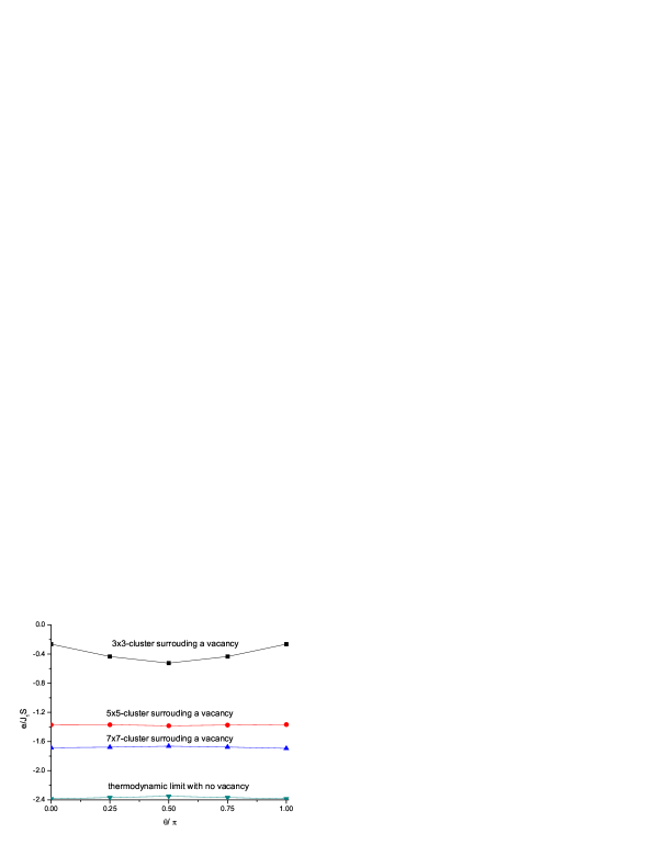
Figure 2: (color online) The $\theta$-dependence of energy per spin in the presence of single vacancy for three different size of clusters: $3\times 3$, $5\times 5$ and $7\times 7$. The parameters are chosen as $J_{2}=J_{1}=1$ and $S=1$.

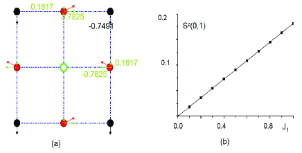
Figure 3: (color online) (a) The magnetic moment configuration around the vacancy in $3\times 3$ cluster with $J_{1}=J_{2}=1$ and $S=1$. (b) The $J_{1}$-dependence of $S^{z}_{(1,0)}$ and $S^{z}_{(0,1)}$ for $S=1$ and $J_{2}=1$.

The above study of a single vacancy suggests that the A-CAFM configuration is favored if only the energy on the small sublattice surrounding the vacancy is considered. In order to confirm that the existence of the global phase transition in the presence of vacancies, we take a super unit cell in the square lattice with $N\times M$ sites and creates one vacancy in the unit. Thus, if we repeat this unit to create a superlattice, we obtain a system in which the percentage of vacancy concentration is given by $\frac{1}{N\times M}$. In this superlattice system, for a given wavevector $k$, the Eq.(Collinear to Anti-collinear Quantum Phase Transition by Vacancies) can be reduced to equations that only couple $2N\times M$ Green functions given by $G_{k+Q_{n,m},k}$ and $F_{k+Q_{n,m},k}$, where $Q_{n,m}=(2\pi n/N,2\pi m/M)$ and $n(m)=0,...,N(M)-1.$ In Fig.4, we show the energy of three different supperlattices as a function of $\theta$ for $J_{1}=J_{2}$ and $S=1$. For both superlattices with $2\times 4$ and $2\times 6$ unit cells which are corresponding to $12.5\%$ and $8.4\%$ vacancy concentration respectively, the anti-collinear state is favored. However, the CAFM state is favored in a superlattice with $4\times 4$ unit cell corresponding to $6.3\%$ vacancy concentration. This result justifies our previous rough estimation of the critical vacancy density.

Figure 4: (color online) The energy of three different superlattices as a function of $\theta$ for $J_{1}=J_{2}$. For the $4\times 4$ lattice, the energy minimum becomes $\theta=0$.

Our above results have important implications in iron-based superconductors. All of our above calculations demonstrate an existence of quantum phase transition from a CAFM state to an A-CAFM state at a certain critical vacancy concentration $\rho_{c}$. While the CAFM state breaks $C^{4}$ rotation symmetry, the A-CAFM state does not break $C^{4}$ rotation symmetry. In iron-pnictides, there is always a tetragonal-to-orthorhombic structural transition which occurs at the temperature above or equal to CAFM transition temperature. This structural transition breaks $C^{4}$ to $C^{2}$ and is naturally explained as a consequence of magnetic fluctuations associated with the CAFM state Fang2008d ; Xu2008a . If the A-CAFM state exists and the structural transition is magnetically driven, our results predict that the lattice distortion can be absent in the A-CAFM phase.

It is also worth to discuss that the vacancy orderings have been observed in $(A_{1-y}Fe_{2-x}Se_{2})$ iron-chalcogenides, where the vacancy patterns are corresponding to a natural reduction of the magnetic frustration so that the magnetic transition temperature is strongly enhanced Fang2011d . The vacancy superlattices used in our calculation do not reduce the magnetic frustration. Therefore, our results do not directly apply to the observed vacancy patterns, such as the 245 pattern in $K_{2}Fe_{4}Se_{5}$ Bao2011a . However, for the materials with very diluted vacancy concentration, we expect that our result should be valid as well.

In summary, we study static vacancies in the collinear magnetic phase of a frustrated Heisenberg $J_{1}$-$J_{2}$ model and identify a quantum phase transition between collinear antiferromagnetic state (CAFM) and an anti-collinear antiferromagnetic phase (A-CAFM). Our results can help to resolve the relation between magnetic and structural transitions in iron-based superconductors.

Acknowledge JPH thanks S. Kivelson for initiating the main idea in this paper and for useful guide and discussion. This work was supported by NSFC under grants Nos. 10874235, 10934010, 60978019, the NKBRSFC under grants Nos. 2009CB930701, 2010CB922904, and 2011CB921502.

References

(1) C. Fang et al, Phys. Rev. B 77, 224509 (2008).
(2) Q. Si, and E. Abrahams, Phys. Rev. Lett. 101, 076401 (2008)
(3) C. Xu, M. Muller, and S. Sachdev, Phys. Rev. B 78, 020501 (2008).
(4) T. Yildirim, Phys. Rev. Lett. 101, 057010 (2008).
(5) C. de la Cruz et al., Nature 453, 899 (2008).
(6) P. Cheng, B. Shen, J. Hu, and H. H. Wen, Phys. Rev. B 81, 174529 (2010).
(7) J. Guo et al., Phys. Rev. B 82, 180520 (2010).
(8) M. Fang et al., ArXiv:1012.5236 (2010).
(9) R. H. Liu et al., ArXiv:1102.2783 (2011).
(10) W. Bao et al., ArXiv:1102.0830 (2011).
(11) J. Bacsa et al., ArXiv:1102.0488 (2011).
(12) V. Y. Pomjakushin et al., ArXiv:1102.1919 (2011).
(13) Z. Wang et al., ArXiv:1101.2059 (2011).
(14) P. Zavalij et al., ArXiv:1101.4882 (2011).
(15) A. M. Zhang et al., ArXiv:1101.2168 (2011).
(16) Y. Shimizu et al., Phys. Rev. Lett. 91, 107001 (2003).
(17) S. S. Lee and P. A. Lee, Phys. Rev. Lett. 95, 036403 (2005).
(18) N. Bulut, D. Hone, D. Scalapino, and E.Y. Loh, Phys. Rev. Lett. 62, 2192 (1989).
(19) C. Chen, et al., Arxiv:1010.2917 (to appear in New J. Phys.).
(20) C. L. Henley, Phys. Rev. Lett. 62, 2056 (1989).
(21) P. Chandra, P. Coleman, and A.I. Larkin, Phys. Rev. Lett. 64, 88 (1990).