N II $\lambda\lambda$5668–5712, a New Class of Spectral Features in Eta Carinae

Abstract

We report on the N II $\lambda\lambda$5668–5712 emission and absorption lines in the spectrum of $\eta$ Carinae. Spectral lines of the stellar wind regions can be classified into four physically distinct categories: 1) low-excitation emission such as H I and Fe II, 2) higher excitation He I features, 3) the N II lines discussed in this paper, and 4) He II emission. These categories have different combinations of radial velocity behavior, excitation processes, and dependences on the secondary star. The N II lines are the only known features that originate in “normal” undisturbed zones of the primary wind but depend primarily on the location of the hot secondary star. N II probably excludes some proposed models, such as those where He I lines originate in the secondary star’s wind or in an accretion disk.

1 Introduction

In $\eta$ Car’s broad-line stellar wind spectrum, the high-excitation helium features have different profiles and fluctuate differently from the “normal” lines of H I, Fe II, etc. Most authors now assume that the He I emission depends on photoionization by a hot companion star, see §6 of Humphreys et al. (2008) and references therein. Observed He II emission is most likely excited by soft X-rays from unstable shocks (Martin et al. 2006, but cf. Steiner & Damineli 2004, Kashi & Soker 2007, and Soker & Behar 2006). Features of these types are important because they show direct influences by the secondary star and the wind-wind collision region. The only clear examples have been helium lines, whose source geometry is both complex and controversial. In this paper we report similar characteristics in a set of N II features, which sample lower-ionization gas than the helium lines.

Broad H I and Fe II emission lines represent $\eta$ Car’s stellar wind spectrum that would be present even if the companion star did not exist (Hillier et al., 2001). Their main components always remain close to system velocity (roughly $-8$ km s^-1, Davidson et al. 1997; Smith 2004).

The He I emission lines, by contrast, shift progressively blueward through most of the 5.5-year spectroscopic cycle. When a spectroscopic event occurs they show a more abrupt negative shift, followed by a rapid positive reversal to renew the cycle (see mid panel of Figure 1, and figures in Nielsen et al. 2007). The overall range of variation is about $0$ to $-250$ km s^-1. Evidently these changes represent flows of highly ionized material, modulated by the secondary star. As the secondary moves in its orbit, it progressively illuminates regions with differing velocity fields, and may perturb some of them. The details are model-dependent: compare, e.g., Nielsen et al. 2007; Damineli et al. 2008; Humphreys et al. 2008; Kashi & Soker 2007, 2008; Martin et al. 2006; Davidson et al. 2001a.

He I absorption shows a similar pattern with variations between $-300$ km s^-1 and $-550$ km s^-1. This behavior is mirrored by the puzzling He II $\lambda$4687 emission observed during spectroscopic events (Steiner & Damineli, 2004; Martin et al., 2006). Hydrogen and Fe II lines have components that behave qualitatively like He I, but cannot be measured separately because they overlap the steady “normal” emission profiles.

Until now no other species were found in $\eta$ Car with velocity variations like the helium lines, and without conspicuous steady components. Here we report that lines of the N II $\lambda\lambda$5668–5712 multiplet do match this prescription. They are always present but were not discussed previously because they were weak. They are noteworthy because they depend on a form of excitation by the hot secondary star, but in different regions than the He I lines. They seem reasonable in some models, but are difficult to explain in others. For example, models where the helium emission originates in a small region close to the secondary star have difficulties in this respect; see §4 below.

Historically, hot windy objects such as P Cygni show strong N II emission and absorption (e.g., Beals 1935; Struve 1935; Swings & Struve 1940). Since nitrogen is abundant in $\eta$ Car’s CNO-processed wind, Hillier et al. (2001) expressed surprise that N II is not more conspicuous there. Some of the features discussed below were identified by Gaviola (1953), but were too weak to be noted by Thackeray (1953). More recently they have been detected by Zethson (2001), Damineli et al. (1998), and Nielsen et al. (2009) without discussion. The lines discussed here are physically different from [N II] $\lambda$5756 which has much lower energy levels.

2 Data and Analysis

Ground-based slit spectroscopy of $\eta$ Car was obtained with the Gemini Multi-Object Spectrograph (GMOS) on the Gemini South telescope from 2007 June to 2010 January. Here we only use 20 sets of observations with the B1200 line grating and a 0.5$\arcsec$ slit that cover the spectrum at $\lambda$5700 Å on the star and on FOS4. FOS4 is a position in the SE lobe of the Homunculus (about 4″ southeast of the star) which reflects the star’s polar spectrum while the spectrum in direct view is representative of lower latitudes (Davidson et al., 1995; Zethson et al., 1999; Davidson et al., 2001b; Smith et al., 2003). The spectral resolution was about 1.2 Å or 65 km s^-1. The seeing varied from 0.5″ to 1.5″, so each GMOS spectrum represents a region typically $\sim$ 1″ across. We prepared 2-D spectrograms with the standard GMOS data reduction pipeline in the Gemini IRAF package and extracted 1-D spectra. The pipeline wavelength calibration was improved using the interstellar absorption line at $\lambda$5782 Å; in this paper we use heliocentric vacuum velocities. Further details, unimportant for this paper, will be listed in a later publication (Mehner et al. 2011, in preparation).

Eta Car was observed with the Hubble Space Telescope Space Telescope Imaging Spectrograph (HST STIS) from 1998 to 2004 and then again starting in 2009. Here we only use observations with the G750M grating, the 52″$\times$0.1″ slit, and central wavelength $\lambda$5734 Å. The spectral resolution was about 1.1 Å or 60 km s^-1. The 1998–2004 observations include a variety of slit positions and orientations. 2009 June and December data cover a region up to 1″ from the central source with parallel slit positions offsets of 0.1″. The long-exposure 2009 data were obtained in HST programs 11506 and 12013, whose PI’s were K. S. Noll and M. Corcoran. The data were reduced using routines developed by the HST Treasury Project that include several improvements over the normal STScI pipeline and standard CALSTIS reductions. We extracted spectra 0.1″ wide.

3 Results

In the GMOS data we found broad emission and absorption lines of the N II $2s^{2}2p3s$ ³P^o – $2s^{2}2p3p$ ³D multiplet at $\lambda\lambda$5668–5712 Å, exhibiting radial velocity variations during the 2009 spectroscopic event similar to the helium lines; see Figure 1 and Table 1. Figure 2 shows the energy levels involved. Note that the lower level, $2p3s$ ³P^o, is more than 18 eV above the N II ground level but is connected to it by a permitted transition. We discuss the excitation mechanism below.

Figure 1 compares spectra of $\eta$ Car obtained from 2007 June to 2010 January showing N II $\lambda$5668, He I $\lambda 4714$, and He II $\lambda 4687$. Weak N II $\lambda\lambda$5668–5712 emission and absorption is always present in the spectrum of $\eta$ Car. The maximum strength of the absorption component has a radial velocity of about $-300$ km s^-1 with respect to the emission peak. During the 2009 spectroscopic event, emission and absorption features shifted about $250$ km s^-1 towards the blue, simultaneous with the He I emission and absorption lines and the He II $\lambda 4687$ emission.

HST STIS data obtained in 2009 June and December clearly show the N II $\lambda\lambda$5668–5712 lines, see Figure 3. In retrospect the faint N II spectral features can also be detected in HST STIS data from 1998–2004, but due to lower S/N they failed to attract notice before. Like the He I absorption, N II absorption was much weaker before 2003; less than 30% compared to 2009 (compare Mehner et al. 2010b). The absorption strengths of both species increased gradually over the last 10 years except during the 2003.5 and 2009.0 spectroscopic events. We determined the “stellar continuum” by a loess (locally weighted scatterplot smoothing) fit to the spectrum and find that the N II absorption is stronger than the emission. (The same is true for P Cygni; Beals 1935, Struve 1935). Gemini GMOS data appear to indicate the opposite, but their data quality is too low to determine a reliable continuum, and ground-based spectra are contaminated by narrow emission lines from ejecta outside the wind, e.g., [Fe II] $\lambda$5675 blends with the N II $\lambda\lambda$5678,5681 absorption. Although we first noticed these features in GMOS data, the high spatial resolution of HST data is essential for examining their character.

Most other permitted N II lines are too weak or blended with emission lines from the wind or nearby ejecta to be observed. However, we see similar behavior in the N II $2p3s$ ³P^o – $2p3p$ ³P series at $\lambda\lambda$4603,4608 Å (Fig. 2). Transitions of the N II $2p3s$ ³P^o – $2p3p$ ³S series are too weak and blended with other lines.

Radiative excitation of level $2s^{2}2p3s$ is very important as discussed later. The $2s2p^{3}$ levels are excited in the same way but lead to no observable results. Transitions from $2s2p^{3}$ ³S^o to $2s^{2}2p3p$ ($\lambda\lambda$6435–7265 Å) have small oscillator strengths and are therefore not observed. STIS data indicates the weak presence of the singlet N II $\lambda$3996 line but this line is blended with others in Gemini data and therefore the identification is not certain. Lines whose upper levels are above the $2p3p$ state like N II $\lambda$5007, even though they are strong in the laboratory, are not observed.

The N II lines and their velocity shifts can also be seen in the reflected polar spectrum at location FOS4, the location decribed in §2. The velocity shifts from the FOS4 separate direction may cast doubt on orbit models, but this question is too complex to discuss here.

4 Line Formation and Significance

The same N II lines are seen in early type stars. In objects like P Cygni and shells of O-stars, $2p3s$ ¹P^o – $2p3p$ ¹S,¹P,¹D and $2p3s$ ³P^o – $2p3p$ ³S,³P,³D are very strong (Swings & Struve, 1940). Large differences between WN stars indicate that these lines are sensitive to atmospheric conditions and/or the variability of the wind. They may also be very sensitive to the FUV flux since they are likely produced via continuum fluorescence (Herald et al., 2001).

In the case of $\eta$ Car the N II absorption and emission almost certainly occur in the primary star’s dense wind, for reasons noted later below. But three facts indicate that UV photons from the secondary star populate the critical $2p3s$ level. (1) The velocity behavior described in §3 strongly suggests some relation to the secondary, analogous to the He I features. (2) The $2p3s$ levels are about 18.5 eV above the ground state, a high value for the primary star’s wind. According to Hillier et al. (2001), the opaque-wind photospheric temperature is below $15,000$ K and emission-line regions in the primary wind are mostly below $10,000$ K; much cooler than the O stars and WR objects mentioned above. The hot secondary star, on the other hand, produces a large flux of 18.5 eV photons (Fig. 10 in Mehner et al. 2010a). (3) This hypothesis appears quantitatively successful as outlined below. Any of these clues by itself might be debatable, but together they seem compelling to us.

Let us summarize an order-of-magnitude assessment of the absorption line strengths that one would expect in a simple model. For simplicity we include only the N⁺ ground level ‘1’ ($2p^{2}$ ³P) and one excited level ‘2’ ($2p3s$ ³P^o); our initial goal is to estimate the equilibrium population ratio $n_{2}/n_{1}$. A two-level system is justified because no permitted transitions connect level 2 to intermediate levels. Consider a uniformly-expanding local volume in the primary wind. Denote the incident continuum photon flux at $h{\nu}_{12}\approx 18.5$ eV by ${\Phi}_{\nu}$, not corrected for line absorption in the gas. As explained in §8.5 in Lamers & Cassinelli 1999 and §8 in Martin et al. 2006, the Sobolev approximation allows us to write expressions for the radiative $1\rightarrow 2$ excitation rate and the re-emission photon escape probability, as functions of the local expansion rate, a line profile function, and atomic parameters. The effective de-excitation rate is proportional to the escape probability, and the most complicated factors appear similarly in both the excitation rate and the escape probability. Consequently the equilibrium population ratio is simple:

$$\frac{n_{2}}{n_{1}}=\frac{g_{2}}{g_{1}}\cdot\frac{{\lambda}_{12}^{2}{\Phi}_{\nu}}{8\pi}\;,$$ (1)

where $g_{1}$ and $g_{2}$ are the statistical weights. This expression remains valid when we take fine structure into account. The same ratio would be found in an LTE case where ${\Phi}_{\nu}/c$ is the Planckian photon density at $h{\nu}_{12}\approx 18.5$ eV. Above we mentioned triplet levels of N II, but singlet levels would also be excited in the same way from $2p^{2}$ ¹D.

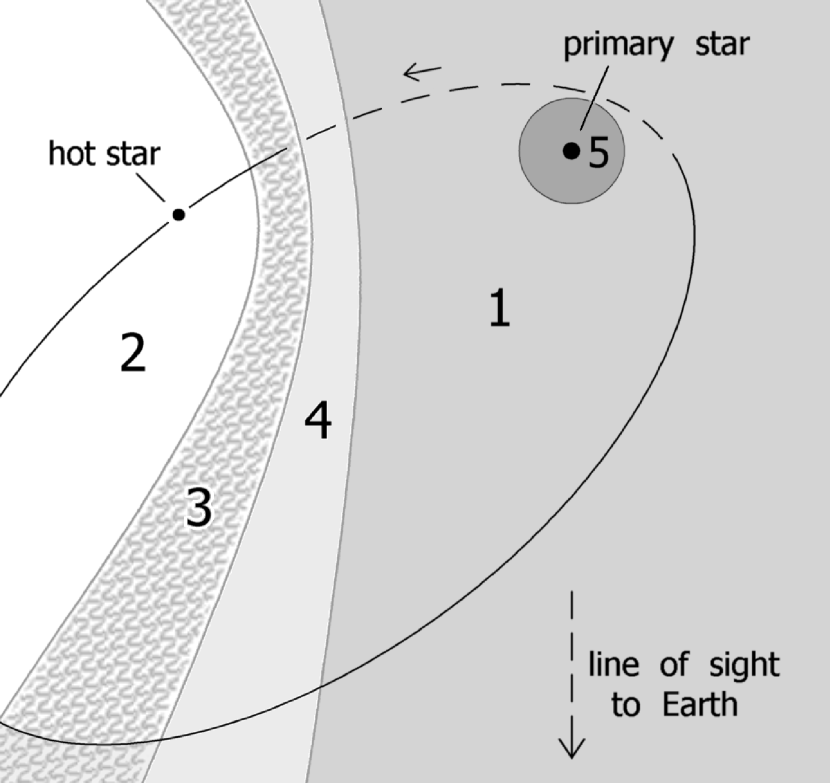
Figure 4: Schematic arrangement of a conventional model for the 2009 June observations. The line of sight to Earth lies in the plane of the Figure, and the secondary star’s orbit is shown projected onto that plane. Regions 1 and 2 are undisturbed parts of the primary and secondary winds. The shocked wind-wind collision region is labeled 3, while region 4 is a He II zone in the primary wind, photoionized by the secondary star. N II is abundant in region 1 but zones 2–4 are more highly ionized. Region 5 is within the opaque-wind photosphere at visual wavelengths. The area shown is roughly 25 AU across, but all details are simplified and idealized.

With conventional parameters for the two stars and their winds, ${\Phi}_{\nu}$ at 18.5 eV is dominated by the hot secondary star. Reasonable values for it are $T_{\mathrm{eff}}\approx 40,000$ K, $R\approx 13\;R_{\odot}$ and $L\approx 4\times 10^{5}\;L_{\odot}$ (Mehner et al., 2010a). According to a WM-basic atmosphere model (Pauldrach et al., 2001), such an object emits roughly $5\times 10^{33}$ photons Hz^-1 s^-1 at $h{\nu}=18.5$ eV, about 30% less than a $40,000$ K blackbody. Figure 4 shows the probable geometry. With the type of orbit model that most authors currently favor (e.g., Okazaki et al. 2008), the separation between stars was about 13 AU when $\eta$ Car was observed in 2009 June. The secondary star was then located roughly 1–5 AU closer to us than the primary, and roughly 10 AU from our line of sight to the primary – depending on the poorly known orbit orientation, of course. With these parameters, eqn. 1 gives $n_{2}/n_{1}\approx 3\times 10^{-8}$ at relevant locations between us and the primary star, i.e., in gas located about 10 AU from the secondary star. The equivalent excitation temperature is near $12,500$ K.

The observed absorption lines have some geometrical complications. Since the opaque-wind photosphere is diffuse with a substantial size, a relevant “line of sight” can be any sample ray in a cylinder with diameter $\sim$ 7 AU (Fig. 4). Strong $2p3s$–$2p3p$ absorption occurs in regions that optimize a combination of attributes: (1) the inner wind is favored because of its high densities; (2) most of the nitrogen must be singly ionized; (3) the N⁺ must be fairly close to the secondary star in order to maximize $\Phi_{\nu}$; and (4) the light path (possibly indirect, due to Thomson scattering) must pass close enough to the primary star to sample continuum radiation from its semi-opaque inner wind. Thus, in Fig. 4, we expect the strongest absorption to occur near and above the symbol ‘1’ that labels Region 1. The picture obviously changes as the secondary star moves along its orbit.

Most nitrogen in the primary wind is singly ionized, due to both the primary and the secondary radiation field (Hillier et al., 2001). Helium in zones 3 and 4 of Fig. 4 provides the shielding which prevents the secondary radiation field from ionizing N⁺ into N⁺⁺, but which allows the 18.5 eV radiation to penetrate. Suppose the primary mass-loss rate is $3\times 10^{-4}$ $M_{\odot}$ yr^-1 and nearly all the CNO is nitrogen (Davidson et al., 1986; Dufour et al., 1999). Then the column densities outside $r=4$ AU (for example) are

$$N(\mathrm{N}^{+})\;\sim\;2\times 10^{20}\;\mathrm{cm}^{-2}\,,$$

$$N(\mathrm{N}^{+}\,2p3s)\;\sim\;6\times 10^{12}\;\mathrm{cm}^{-2}\,.$$

This column density would produce a combined equivalent width of about 1 Å for the $\lambda$5681.14 and $\lambda$5677.60 Å absorption lines. Since this exceeds the observed value of 0.5 Å, the proposed mechanism appears to be sufficient, even if only a limited part of the wind is involved. Let us emphasize that the parameter values in this sample calculation were chosen ab initio without knowing what result they would lead to; there was no readjustment to get a desired outcome. Note that the margin of error does not allow much smaller values of ${\Phi}_{\nu}$ and gas densities.

The emission features reported in §3 are comparable in strength to the absorption – probably weaker and certainly not much stronger – so they resemble the pure scattering case of P Cyg lines. In other words, the observed $2p3s$ – $2p3p$ emission line strengths automatically resemble the absorption strengths. More detailed calculations will require elaborate geometrical models of the ionization and excitation zones.

As we noted earlier, these N II features should arise chiefly in regions of the primary wind that are fairly close to the secondary star, and, therefore, close to the He⁺ zones and wind-wind shocks. If shock instabilities do not distort it too much, the He⁺/He⁰ ionization front is expected to have a pseudo-hyperboloidal shape that may be either concave or convex towards the secondary star (Fig. 4). Adjoining primary-wind zones are spatially large enough to account for the N II lines. Generically, this type of model can explain the velocity variations, but authors disagree about details (e.g., Nielsen et al. 2007; Damineli et al. 2008; Humphreys et al. 2008; Martin et al. 2006).

Far more important than merely being consistent with some models of the $\eta$ Car system, the N II features may disprove others. For example, it has been suggested that the helium lines originate in the acceleration zone of the secondary star’s wind, or perhaps in an accretion disk around the secondary, rather than in the primary wind (Soker & Behar, 2006; Kashi & Soker, 2007; Steiner & Damineli, 2004). But the N II features, with practically the same velocity behavior, almost certainly cannot represent such zones; so models of that type would be forced to explain the He I and N II velocities differently.

The arguments are simplest for absorption lines. First we note that with credible parameters for the two stars (e.g., Hillier et al. 2001; Mehner et al. 2010a), the primary wind accounts for at least 95% of the visual-wavelength continuum, most likely 98–99%. Therefore the absorption features in Fig.  3 definitely represent material located between us and the inner parts of the primary wind. (In other words, blocking the entire secondary star would not produce absorption as deep as that shown in Fig. 3, even if $\tau_{\mathrm{line}}\gg 1$.) Can this absorbing material be part of the secondary wind or an accretion disk of the secondary star? Presumably not; because in every proposed orbit model the relevant lines of sight either miss the secondary star and its wind entirely at most times, or pass through only the outskirts of the secondary wind. Gas densities in the secondary wind are two orders of magnitude less than we used in the calculations outlined above, the nitrogen is mainly N III, and the velocity dispersion is too large for the observed absorption features. This type of model would badly fail the quantitative feasibility test that the “conventional” model passed. Regarding the N II emission features, they are fairly weak relative to the total observed continuum, but would be extraordinarily strong compared to the visual-wavelength continuum of just the secondary star.

Developing these arguments further would be beyond the scope of this paper; our main point is that the N II lines convey information that is not available in other spectral features. This is mainly because they arise in “normal” parts of the primary wind but they are sensitive to the current location of the secondary star. Helium lines also depend on UV from the secondary, but their emission zones are extremely difficult to model since they depend on the unstable primary shock, post-shock cooling, local ”clumping,” etc. In principle the N II zones are expected to be much steadier, and the excitation mechanism is relatively insensitive to inhomogeneities. For these reasons the N II features may be good indicators of average density in the wind combined with the secondary star’s orbital motion. In particular one might expect their velocities to be easier to model than those of helium lines.

If the “conventional” model is more or less valid, then the N II absorption features should weaken around apastron when $\Phi_{\nu}$ is smallest. Unfortunately the 2000–2002 HST STIS data (the only previous apastron passage when STIS was available) are not adequate to test this “prediction” easily. Perhaps new STIS observations will be made in 2011–2012.

In §3 we mentioned that He I and N II absorption lines have grown in strength during the past 10 years. At first sight this appears counter-intuitive, since the wind density appears to have decreased (Mehner et al., 2010b). However, the situation has various dependencies that tend to oppose each other so intuition may be a poor guide. Decreasing mass loss rate implies a smaller, denser opaque-wind photosphere; eqn. 1 becomes invalid if continuum absorption destroys the trapped 18.5 eV resonance photons before they escape; etc. This problem merits further attention. As the wind decreases it is conceivable that the primary star may eventually become hot enough to excite these lines in addition to the secondary. Whatever the solution, we expect the N II lines to provide different parameter contraints than the spectral features that are excited in more normal ways.

In summary, spectral features in $\eta$ Car’s wind can be assigned to these categories:

1. The “normal” lines of hydrogen, Fe II, etc. In principle these can be used to analyze the primary wind (Hillier et al., 2001).

2. He I emission and absorption. Most authors agree that these are related in some way to the secondary star, but the details are controversial (see references cited in §1 above).

3. N II emission and absorption. These lines arise in normal-ionization parts of the primary wind, but they depend mainly on the proximity of the secondary star. In this sense they sample a new region of parameter space. In most recent models, the N II zones are much simpler than the ionized helium. We emphasize that the He I lines depend on photoionization, $h\nu>24.6$ eV, whereas the N II lines depend on photoexcitation at $h\nu\sim 18.5$ eV. The ratio $f_{\nu}(>25~{}\mathrm{eV})/f_{\nu}(18.5~{}\mathrm{eV})$ depends strongly on the secondary star’s temperature (WM-basic atmosphere models, Pauldrach et al. 2001).

4. He II $\lambda$4687, an unsolved puzzle not discussed here. It depends on soft X-rays from the colliding-wind region, not UV from the secondary star.

A good basic model for the primary wind and the binary system must account for at least the first three of these, throughout most of the 5.5-year cycle. (He II $\lambda$4687 may depend on shock instabilities too complex for a “basic” model.)

After an earlier version of this paper appeared on astro-ph, Kashi & Soker (2011) have proposed an alternative interpretation of the N II lines. A full response would make this paper too long, but in our view they do not explain how gas in a very small locale near the secondary star can produce substantial absorption lines in the spectrum of the much larger primary-wind photosphere (see discussion above).

Acknowledgements We thank the staff and observers of the Gemini-South Observatory in La Serena for their help in preparing and conducting the observations. We also thank Roberta Humphreys, John Martin, and Kazunori Ishibashi for discussions and helping with non-routine steps in the data preparation.

Figure 1: N II $\lambda$5668, He I $\lambda 4714$, and He II $\lambda 4687$ in spectra of $\eta$ Car obtained with Gemini GMOS from 2007 June to 2010 January. Days before and after the 2009 spectroscopic event at MJD 54860 are displayed next to each tracing. Arrows indicate the zero velocities of the emission lines. Note that most of the 5.5 year cycle is represented by the top two and bottom two samples and that [Fe II] $\lambda$5675 blends with the N II $\lambda\lambda$5678,5681 absorption.

Figure 2: The lowest triplet levels of N II. Odd-parity levels such as $2s^{2}2p3s$ ³P^o are marked with small ‘o’s. In this paper we concentrate on the $2s^{2}2p3s$ – $2s^{2}2p3p$ transitions because they have observationally convenient wavelengths, see §3.

Figure 3: N II $\lambda\lambda$5668–5712 in HST STIS data from 2009 June. Zero velocity emission and absorption at $-300$ km s^-1 are indicated with brackets. The dashed curve represents the stellar continuum. HST’s high-spatial resolution shows the absorption much better than ground-based data. The strong N II $\lambda\lambda$5678,5681 absorption is blended with [Fe II] $\lambda$5675 in the Gemini spectra.

Table 1: Observed N II $\lambda\lambda$5668–5712 transitions

Wavelength	Transition	Ei	Ek	Aki
(Å)		(cm-1)	(cm-1)	(s-1)
N II 5668.20	$2s^{2}\;2p\;3s$ 3P1 – $2s^{2}\;2p\;3p$ 3D2	148940.17	166582.45	3.45e+07
N II 5677.60	$2s^{2}\;2p\;3s$ 3P0 – $2s^{2}\;2p\;3p$ 3D1	148908.59	166521.69	2.80e+07
N II 5681.14	$2s^{2}\;2p\;3s$ 3P2 – $2s^{2}\;2p\;3p$ 3D3	149076.52	166678.64	4.96e+07
N II 5687.79	$2s^{2}\;2p\;3s$ 3P1 – $2s^{2}\;2p\;3p$ 3D1	148940.17	166521.69	1.78e+07
N II 5712.35	$2s^{2}\;2p\;3s$ 3P2 – $2s^{2}\;2p\;3p$ 3D2	149076.52	166582.45	1.17e+07

References

- Beals (1935) Beals, C. S. 1935, MNRAS, 95, 580
- Corcoran et al. (2010) Corcoran, M. F., Hamaguchi, K., Pittard, J. M., Russell, C. M. P., Owocki, S. P., Parkin, E. R., & Okazaki, A. 2010, ApJ, 725, 1528
- Damineli et al. (2008) Damineli, A., Hillier, D. J., Corcoran, M. F., Stahl, O., Groh, J. H., Arias, J., Teodoro, M., Morrell, N., Gamen, R., Gonzalez, F., Leister, N. V., Levato, H., Levenhagen, R. S., Grosso, M., Colombo, J. F. A., & Wallerstein, G. 2008, MNRAS, 386, 2330
- Damineli et al. (1998) Damineli, A., Stahl, O., Kaufer, A., Wolf, B., Quast, G., & Lopes, D. F. 1998, A&AS, 133, 299
- Davidson (2006) Davidson, K. 2006, in The 2005 HST Calibration Workshop: Hubble After the Transition to Two-Gyro Mode, ed. A. M. Koekemoer, P. Goudfrooij, & L. L. Dressel, 247
- Davidson et al. (1986) Davidson, K., Dufour, R. J., Walborn, N. R., & Gull, T. R. 1986, ApJ, 305, 867
- Davidson et al. (1997) Davidson, K., Ebbets, D., Johansson, S., Morse, J. A., & Hamann, F. W. 1997, AJ, 113, 335
- Davidson et al. (1995) Davidson, K., Ebbets, D., Weigelt, G., Humphreys, R. M., Hajian, A. R., Walborn, N. R., & Rosa, M. 1995, AJ, 109, 1784
- Davidson et al. (2001a) Davidson, K., Gull, T. R., & Ishibashi, K. 2001a, in ASP Conf. Ser., Vol. 233, P Cygni 2000: 400 Years of Progress, ed. M. de Groot & C. Sterken, 173
- Davidson et al. (2001b) Davidson, K., Smith, N., Gull, T. R., Ishibashi, K., & Hillier, D. J. 2001b, AJ, 121, 1569
- Dufour et al. (1999) Dufour, R. J., Glover, T. W., Hester, J. J., Currie, D. G., van Orsow, D., & Walter, D. K. 1999, in ASP Conf. Ser., Vol. 179, Eta Carinae at The Millennium, ed. J. A. Morse, R. M. Humphreys, & A. Damineli, 134
- Gaviola (1953) Gaviola, E. 1953, ApJ, 118, 234
- Herald et al. (2001) Herald, J. E., Hillier, D. J., & Schulte-Ladbeck, R. E. 2001, ApJ, 548, 932
- Hillier et al. (2001) Hillier, D. J., Davidson, K., Ishibashi, K., & Gull, T. 2001, ApJ, 553, 837
- Humphreys et al. (2008) Humphreys, R. M., Davidson, K., & Koppelman, M. 2008, AJ, 135, 1249
- Kashi & Soker (2007) Kashi, A. & Soker, N. 2007, New Astronomy, 12, 590
- Kashi & Soker (2008) —. 2008, MNRAS, 390, 1751
- Kashi & Soker (2009) —. 2009, ApJ, 701, L59
- Kashi & Soker (2011) —. 2011, ArXiv e-prints
- Lamers & Cassinelli (1999) Lamers, H. J. G. L. M. & Cassinelli, J. P. 1999, Introduction to Stellar Winds, ed. Lamers, H. J. G. L. M. & Cassinelli, J. P.
- Martin et al. (2006) Martin, J. C., Davidson, K., Humphreys, R. M., Hillier, D. J., & Ishibashi, K. 2006, ApJ, 640, 474
- Mehner et al. (2010a) Mehner, A., Davidson, K., Ferland, G. J., & Humphreys, R. M. 2010a, ApJ, 710, 729
- Mehner et al. (2010b) Mehner, A., Davidson, K., Humphreys, R. M., Martin, J. C., Ishibashi, K., Ferland, G. J., & Walborn, N. R. 2010b, ApJ, 717, L22
- Nielsen et al. (2007) Nielsen, K. E., Corcoran, M. F., Gull, T. R., Hillier, D. J., Hamaguchi, K., Ivarsson, S., & Lindler, D. J. 2007, ApJ, 660, 669
- Nielsen et al. (2009) Nielsen, K. E., Kober, G. V., Weis, K., Gull, T. R., Stahl, O., & Bomans, D. J. 2009, VizieR Online Data Catalog, 218, 10473
- Okazaki et al. (2008) Okazaki, A. T., Owocki, S. P., Russell, C. M. P., & Corcoran, M. F. 2008, MNRAS, 388, L39
- Pauldrach et al. (2001) Pauldrach, A. W. A., Hoffmann, T. L., & Lennon, M. 2001, A&A, 375, 161
- Smith (2004) Smith, N. 2004, MNRAS, 351, L15
- Smith et al. (2003) Smith, N., Davidson, K., Gull, T. R., Ishibashi, K., & Hillier, D. J. 2003, ApJ, 586, 432
- Soker & Behar (2006) Soker, N. & Behar, E. 2006, ApJ, 652, 1563
- Steiner & Damineli (2004) Steiner, J. E. & Damineli, A. 2004, ApJ, 612, L133
- Struve (1935) Struve, O. 1935, ApJ, 81, 66
- Swings & Struve (1940) Swings, P. & Struve, O. 1940, ApJ, 91, 546
- Thackeray (1953) Thackeray, A. D. 1953, MNRAS, 113, 211
- Zethson (2001) Zethson, T. 2001, PhD thesis, AA(LUNDS UNIVERSITET (SWEDEN))
- Zethson et al. (1999) Zethson, T., Johansson, S., Davidson, K., Humphreys, R. M., Ishibashi, K., & Ebbets, D. 1999, A&A, 344, 211