Supermassive Black Hole Mass Estimates Using Sloan Digital Sky Survey Quasar Spectra at $0.7<z<2$

Abstract

We present Mg ii -based black hole mass estimates for 27,602 quasars with rest-frame UV spectra available in the Sloan Digital Sky Survey Data Release Three. This estimation is possible due to the existence of an empirical correlation between the radius of the broad line region and the continuum luminosity at 3000 Angstroms. We regenerate this correlation by applying our measurement method to UV spectra of low-redshift quasars in the HST/IUE databases which have corresponding reverberation mapping estimates of the H $\beta$ broad line region’s radius. Our mass estimation method uses the line dispersion rather than the full width at half maximum of the low-ionization Mg ii emission line. We measure Mg ii line dispersions for quasars whose spectra have been reconstructed using the most significant eigenspectra produced through Principal Component Analysis. We have tested the reliability of using reconstructed spectra in black hole mass estimation using a Monte Carlo simulation and by comparing the results from original and reconstructed Data Release Three spectra. We show that using reconstructed spectra not only makes bias-free mass estimation possible for quasars with low spectroscopic signal-to-noise ratio, but also reduces the intrinsic scatter of the distribution of the black hole masses to lower than 0.15 dex.

1 Introduction

Over the past decade, we have learned that all large galaxies have supermassive black holes at their centers (e.g., Kormendy & Richstone et al. 1995; Richstone et al. 1998). Material falling onto black holes forms a rapidly spinning disk which heats up and radiates the light we see as quasars and other active galactic nuclei (AGN) (e.g., Salpeter 1964; Zel’dovich & Novikov 1964; Lynden Bell 1969). The masses of these black holes can be measured through different techniques. In galaxies with a dormant black hole, the BH mass can be measured through the velocity dispersion of stars or gas close enough to the BH which their dynamics are dominated by BH gravity (within the radius of influence; e.g., Gebhardt et al. 2000; Ferrarese & Merritt 2000; Tremaine et al. 2002). However, this method cannot be used for active nuclei where the nucleus outshines the core of the host galaxy (e.g., Richstone et al. 1998; Gebhardt et al. 2000; Ferrarese & Merritt 2000; Tremaine et al. 2002). Thus, alternative mass measurement methods are necessary, but are AGN type dependent (Blandford & McKee 1982; Peterson 1993; Miyoshi et al. 1995). In nearly edge-on (Type 2) AGNs, mass can be measured from water masers located in the outer accretion disk (Miyoshi et al. 1995). However, water masers cannot be used widely due to the extreme edge-on alignment needed for radiation to be sufficiently amplified. In more face-on (Type 1) AGNs, one can instead use reverberation mapping when variations of the broad emission lines relative to the continuum are present (e.g., Koratkar & Gaskell 1991; Kaspi et al. 2000; Peterson et al. 2004; Kaspi et al. 2005; Bentz et al. 2006; Bentz 2009).

Reverberation mapping (RM) studies (Blandford & McKee 1982; Peterson 1993) take advantage of long monitoring campaigns of AGNs to infer properties of the broad line emitting region (BLR) through characterization of time delays ($\tau$) between broad emission line and continuum flux variations (e.g., Koratkar & Gaskell 1991; Kaspi et al. 2000; Kaspi et al. 2005; Bentz et al. 2006; Bentz 2009). In principle, RM can generate a velocity-delay map (revealing kinematic structure in the BLR) which can help one to estimate the black hole mass independent of other methods (see Done & Krolik 1996; Ulrich & Horne 1996; Kollatschny 2003; Horne et al. 2004; Denney et al. 2009; Bentz et al. 2009). However, at the moment, one still has to calibrate quasar black hole masses to nearby well studied dormant black holes (assuming that they are descendants of the active BHs; see, e.g., Kaspi et al. 2000; Krolik 2001; McLure & Dunlop 2001; Onken et al. 2004). It has taken many years of RM campaigns to obtain a large sample of such mass measurements even for a handful of low redshift quasars (e.g., Done & Krolik 1996; Ulrich & Horne 1996; Kollatschny 2003; Peterson 2006; Bentz et al. 2009; Denney et al. 2009). The RM results show an empirical correlation between the distance of the BLR from the BH (which is the measured time-lag $\tau$ times the speed of light) and a monochromatic continuum luminosity (known as $R-L$ or $\tau-L$ correlation; Kaspi et al. 2000; Bentz et al. 2006). This $R-L$ correlation simplifies the mass measurement since determining the radius of the BLR using long monitoring campaigns can be replaced by measuring the monochromatic continuum luminosity from a single epoch spectrum.

The RM results also show a relationship between emission line widths ($\Delta V$) and corresponding time-lags (e.g., Peterson & Wandel 1999, 2000; Onken & Peterson 2002; Kollatschny 2002) which confirms the virialization of the BLR. This relationship enables a secondary method of BH mass determination from $\frac{GM}{R}\propto(\Delta V)^{2}$ if one assumes that the $\Delta V$ of a virialized emission line (e.g., H $\beta$) reflects the virialized bulk motion of the emitting gas (e.g., Peterson & Wandel 1999, 2000; Onken & Peterson 2002; Kollatschny 2003). By measuring the line width of a particular line (using the FWHM or the line dispersion) and the luminosity of the AGN at a particular wavelength, one can calibrate the virial mass equation of the secondary method for a sample of RM black hole masses. That equation can then be used to estimate unknown quasar BH masses (e.g., Wandel et al. 1999; Vestergaard 2002; McLure & Jarvis 2002; Woo & Urry 2002; Vestergaard & Peterson 2006; Shen et al. 2008; Wang et al. 2009).

Much work on distant black hole mass estimates has used the hydrogen H $\beta$ emission line and the 1549 Å doublet of triply ionized carbon (C iv); e.g., Kaspi et al. (2000), Vestergaard (2002), McLure & Jarvis (2002) and Vestergaard & Peterson (2006). H $\beta$ can be identified in low redshift quasars ($z\lesssim 0.8$) with observations from ground-based telescopes in the optical or near infrared, while the C iv emission line can be identified in high redshift quasars ($z\gtrsim 2$) in those bands. Thus, H $\beta$ provides well calibrated masses but cannot be seen in the most distant black holes with ground based telescopes, while C iv can be seen but could be strongly contaminated by non-gravitational motions. For example, the peak of the C iv emission line is usually blueshifted, probably implying an outflow of material (e.g., Leighly et al. 2000; Yuan et al. 2004; Vestergaard 2009).

We have assembled a catalogue of black hole mass estimates using the 2798 Å doublet of singly ionized magnesium (Mg ii), which can be observed by ground-based telescopes in the optical or near infrared for even the most distant quasars and which is thought to probe largely the same region of the accretion disk as H $\beta$ (McLure & Jarvis 2002; but see Wang et al. 2009). Although there is no RM study which demonstrates the virialization of the Mg ii emission line, BH mass estimates using Mg ii show consistency with similar estimates using H $\beta$ (McLure & Jarvis 2002), which is considered a virialized line (Peterson & Wandel 1999).

For our mass estimates, we use the line dispersion of the line profile instead of FWHM since the relation between rms line dispersion and RM time-delay appears to be less scattered than the same relation with rms FWHM, at least for the H $\beta$ line (Peterson et al. 2004). The line dispersion uses the data directly but is sensitive to the wings of the line profile (Collin et al. 2006). The FWHM is the FWHM of a fit of one or more Gaussians to the line profile (e.g, McLure & Dunlop 2004; Shen et al. 2008), and the FWHM of a single Gaussian fit in particular may be a poor representation of the true FWHM of a line. Furthermore, it is not confirmed that the Mg ii FWHM is linearly related to the rms FWHM of H $\beta$ (Wang et al. 2009). Shen et al. (2008) have provided a BH mass catalogue with mass estimates made using the FWHMs of Mg ii, H $\beta$ and C iv. However, they have not calibrated the Mg ii scaling relation but instead have adopted the McLure & Dunlop (2004) relationship, despite there being many updated RM mass measurements since 2004. Onken & Kollmeier (2008) have shown that the Shen et al. (2008) Mg ii mass estimates are Eddington ratio dependent, which may indicate a problem with FWHM-based Mg ii mass estimates. We are therefore motivated to test the alternative, the line dispersion of Mg ii.

To reduce the uncertainties in the line dispersion due to low signal-to-noise ratio spectra and the sensitivity of the technique to the line wings, we have reconstructed the quasar spectra using the Karhunen-Loève transformation technique (also called Principal Components Analysis; PCA) e.g., Boroson and Green (1992); Connolly et al. (1995); Yip et al. (2004); Boroson et al. (2010). Reconstructing the quasar spectra reduces the noise sufficiently for us to use the line dispersion robustly.

The outline of this paper is as follows. In §2, we describe how we measure the second moment of the Mg ii line profile, including how we model Fe ii emission lines and establish a local continuum. In §3, we calibrate a mass scaling relation using the Mg ii line dispersion and the monochromatic continuum luminosity at 3000Å. In §4, we describe how we select our data sample from the SDSS. In §5, we explain how we reduce the noise level by reconstructing the SDSS quasar spectra using PCA. In §6, we study the effect of the radiation pressure on BH mass estimates and calibrate a new mass scaling relation for that scenario. In §7, we simulate the effects of noise in reconstructed spectra to understand the biases on BH mass estimates before and after reconstruction. In §8, we use the mass scaling relations to estimate the BH masses of SDSS quasars and present our BH mass catalogue. We then compare our BH mass estimates with Shen et al. (2008). In §9, we present our conclusions.

In this study we assume a Lambda Cold Dark Matter ($\Lambda CDM$) cosmology with Hubble constant $H_{0}=71$ km s^-1 Mpc^-1, fractional dark energy density $\Omega_{\Lambda}=0.74$ and fractional matter energy density $\Omega_{m}=0.26$ (Spergel et al. 2007) to calculate necessary cosmological quantities.

2 Black Hole Mass Estimates via Secondary Method

To compute $\mathcal{M}_{\textrm{BH}}$ from the virial equation

$$\mathcal{M}_{\textrm{BH}}=\frac{\bar{f}R_{BLR}(\Delta V)^{2}}{G}.$$ (1)

it is necessary to estimate the radius of the broad line region, $R_{BLR}$, via a correlation with the AGN continuum luminosity when there is no reverberation mapping data available. The observed line width, $\Delta V$, and the continuum luminosity can both be estimated from a single epoch spectrum. The average geometrical factor $\bar{f}$ will remain as a free parameter to be adjusted such that it makes these secondary mass estimates most consistent with the virial mass estimates. The virial masses are in turn calibrated to direct mass measurements of nearby inactive black holes through the BH mass - bulge velocity dispersion ($\mathcal{M}_{\textrm{BH}}-\sigma_{\star}$) relationship (e.g., Gebhardt et al. 2000; Ferrarese & Merritt 2000; Tremaine et al. 2002). This calibration is valuable since there is no direct way to estimate the mass zero point for the quasar BH mass relationship, but it does assume that the same relationship is valid for quasars and for inactive BHs.

2.1 Measuring the Line Width of an Emission Line

The traditional way to measure the line width is to measure its FWHM. This is simple for single peaked lines and more complex for multiple-peaked lines or noisy data (for double-peaked lines, there is a complete discussion in Peterson et al. 2004). The line dispersion, which can be calculated without making any assumption about the line profile, can be defined by:

$$\sigma^{2}_{line}(\lambda)=<\lambda^{2}>-\lambda_{0}^{2}$$ (2)

where $<\lambda^{2}>$ and $\lambda_{0}$ are the $2^{nd}$ & $1^{st}$ moments of the emission line profile $P(\lambda)$:

$$<\lambda^{2}>=\frac{\int\lambda^{2}P(\lambda)d\lambda}{\int P(\lambda)d\lambda}$$ (3)

$$\lambda_{0}=\frac{\int\lambda P(\lambda)d\lambda}{\int P(\lambda)d\lambda}.$$ (4)

The second moment is more sensitive to blending with other lines or extended wings than the FWHM, but less sensitive to the presence of even strong narrow-line components. The FWHM versus time lag plots for emission lines show dramatic scatter (especially for H $\beta$) when using the mean spectra (which are more similar to single epoch spectra than rms spectra are), while the line dispersion, $\sigma_{line}$, versus time lag plots show less scatter (Peterson et al. 2004).

On the other hand, studies of RM samples have shown that AGNs with line dispersion, $\sigma_{line}$, lower than 2000 km s^-1 have $\textrm{FWHM}/\sigma_{line}<2.35$ while AGNs with $\sigma_{line}>2000$ km s^-1 have $\textrm{FWHM}/\sigma_{line}>2.35$ (Sulentic et al. 2000; Collin et al. 2006; Peterson et al. 2007). In particular, Peterson et al. (2007) report that the observed value of $\textrm{FWHM}/\sigma_{line}$ for a sample of RM AGN ranges between $\sim 0.71$ and $\sim 3.45$ with an average value of $\sim 2.0$. This result clearly indicates the non-Gaussianity of line profiles for quasar emission lines. Thus using the FWHM as a line width indicator may overestimate the BH masses for the broadest emission lines and underestimate the BH masses for the narrowest emission lines as compared to BH mass estimates using the line dispersion.

The true line dispersion can be determined through considering the instrumental resolution and writing the observed line width in terms of the intrinsic line dispersion, $\sigma_{intr}$ and the spectrograph’s instrumental line profile, $\sigma_{inst}$:

$$\sigma^{2}_{line}=\sigma^{2}_{intr}+(1+z)^{-2}\sigma^{2}_{inst}$$ (5)

where the instrumental dispersion is observed-frame while the other two are rest-frame. The instrumental resolution of an SDSS spectrum is a function of plate, fiber, and wavelength. The wavelength dispersion in pixels as a function of wavelength for each fiber on a plate is stored in HDU #4 of the spPlate FITS files. For our objects, we need to know the instrumental dispersion at the observed wavelength of Mg ii. For each quasar, the observed wavelength of Mg ii is calculated as $\lambda_{o}=2800.26(1+z)$. Using the spPlate file, the corresponding pixel in the quasar’s SDSS spectrum is located and the wavelength dispersion $d$ (in units of pixels) at that pixel is extracted. The pixel scale is $10^{-4}\ln(10)\lambda_{o}$ Å/pixel, so the instrumental dispersion in Å is given by $2.302585\times 10^{-4}\lambda_{o}d$.

2.2 Fitting Method

The rest-frame ultraviolet spectrum of an AGN can be approximated as a power-law continuum plus broad and overlapping Fe ii emission and broad emission lines from other ions such as Mg ii. To measure the Mg ii line, we must remove the contaminating Fe ii emission from AGN spectra. We subtract a best-fit Fe ii template and power law continuum estimate, which together form what is called a pseudo-continuum.

To match the Fe ii lines to the AGN spectra, we build an Fe ii model by convolving the Fe ii template generated from the nearby AGN I Zw 1 by Vestergaard & Wilkes (2001) with a Gaussian. The AGN spectra have lower resolution than the Fe ii template so we rebin the Fe ii template to match the AGN spectra in their rest frames. Vestergaard & Wilkes (2001) has been the standard empirical Fe ii template since its publication. Tsuzuki et al. (2006) present a new template, also derived from I Zw 1, which unlike that of Vestergaard & Wilkes (2001) shows some Fe ii emission at wavelengths 2780-2920 Å where confusion with Mg ii is an issue in constructing a template. While some such Fe ii emission is certainly present, Tsuzuki et al. (2006) derive their Fe ii template by assuming Gaussian line profiles for Mg ii in I Zw 1. What they interpret as Fe ii emission at 2790 Å could instead be a weak blue wing of Mg ii emission. Furthermore, neither the theoretical Fe ii spectra considered by Tsuzuki et al. (2006) nor those presented by Bruhweiler & Verner (2008) show strong evidence for emission at wavelengths corresponding to features at 2780-2920 Å in the Tsuzuki et al. (2006) template. More work on Fe ii templates is clearly needed, but meanwhile we will use the Vestergaard & Wilkes (2001) template.

The normalization and slope of the power law continuum are initially estimated using two normalization windows, $2238-2248$ Å and $3014-3027$ Å, which are the least contaminated from Fe ii or other lines (Vestegaard and Wilkes 2001).

To allow improvement in the fitting quality we scale the Fe ii template independently above and below $2800$Å. This additional amplitude will be accepted if the new $\chi^{2}$ is lower than the 95% confidence lower limit on the old $\chi^{2}$ with only 4 free parameters. The best pseudo-continuum is then subtracted from the AGN spectra.

We vary the amplitude and slope of the power law continuum, the amplitude of the Fe ii template above and below $2800$Å, and the width of the Gaussian convolved with the Fe ii template to find the best fit. Using a nonlinear Levenberg-Marquardt least-squares fitting method, we calculate the minimum $\chi^{2}$ value for the three fitting windows $2192-2400$ Å, $2445-2724$ Å, and $2867-3027$ Å chosen to avoid the [Ne iv] $\lambda$2423 Å and Mg ii $\lambda$2798 Å emission lines during the Fe ii and continuum estimation.

3 Determining the Mass Scaling Relationship

To determine a mass scaling relationship which uses $\sigma_{MgII}$ and $\lambda L_{3000}$, we first need to investigate the existence of a relationship between $\lambda L_{3000}$ and $R_{BLR}$. If that relationship exists then we can scale our mass relationship to an existing sample of BH masses to determine the geometrical factor.

The most direct measurements of the central black hole masses of powerful AGN come from the reverberation mapping studies of $17$ Seyferts and $17$ PG quasars by Wandel, Peterson & Malkan (1999) and Kaspi et al. (2000), respectively. These studies are based on the time lag measurement between the variation of the AGN continuum and the broad emission line H $\beta$ of local AGN (low redshift objects with $z<0.4$). We thus use this sample as our reference for the scaling process.

We select $21$ objects from this sample (Table 1 of McLure & Jarvis 2002) for which the Mg ii FWHM has been calculated. We also have FWHM and H $\beta$ line dispersion measurements for the same objects from Peterson et al. (2004).

This list of AGN consists of 5 high resolution spectra from the Hubble Space Telescope (HST) Faint Object Spectrograph (FOS) and 16 low resolution spectra from the International Ultraviolet Explorer (IUE) Long-Wavelength Prime (LWP) spectrograph (see Table 1). For most of them there is more than one observation. In order to increase the signal-to-noise ratio and sometimes to increase the wavelength coverage, we combine different observations of each object by using a weighted average method. We adopt as the time-lag to the Mg ii BLR the weighted average time-lag estimated using H$\alpha$, H$\beta$ and H$\gamma$, or whichever subset of those three are available, from Peterson et al. (2004). While these lines sometimes have different timelags, in this case the small number of H$\alpha$ and H$\gamma$ measurements available means that the resulting correlation is not significantly different if only the H$\beta$ timelags are used.

By using our fitting procedure, we find the best-fit broadened Fe ii template and the best power law continuum for each spectrum in Table 1 to create the corresponding pseudo-continuum. We subtract this pseudo-continuum from the spectrum so that we measure the line dispersion of the Mg ii from the isolated emission line. The line dispersion for Mg ii, $\lambda L_{3000}$, and the virial mass estimate can be seen in Table 1 column 3, 4, and 8 respectively.

In a second approach, we use PCA-reconstructed spectra instead of raw spectra (see § 5 for details). However, using reconstructed spectra with high SNR does not improve the $\tau-\lambda L_{3000}$ correlation significantly.

We estimate the slope and intercept of the linear correlation between the logarithms of $\tau_{BLR}$ and $\ell\equiv\lambda L_{3000}/10^{44}$ erg s^-1 using several fitting techniques. However, we eliminate some of the objects from our list based on a large relative error of the average time-lag, $\Delta\tau_{average}/\tau_{average}>31.7\%$. These objects are 3C390.3, PG$0844+349$, PG$1229+204$, NGC4051 and 3C120.

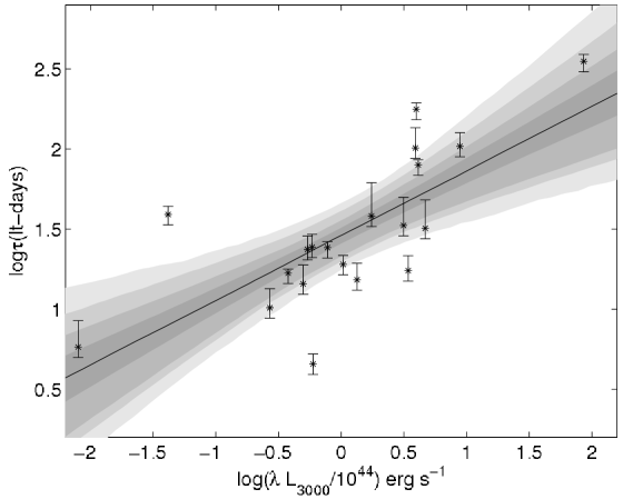
Figure 1: The best linear fit to the reference sample in Table 1 using Markov Chain Monte-Carlo Simulation (MCMC; Haario et al. 2006) method with $33\%$ intrinsic scatter. The gray areas correspond to: 50%, 90%, 95% and 99% posterior regions.

Both the FITEXY (Tremaine et al. 2002; Press et al. 1992) and BCES methods (Akritas et al. 1996) gave a slope consistent with 0.5 within $\approx 1\sigma$, with 20% uncertainty in the best case (see Table 2). Given those results, and because a slope of 0.5 matches the theoretical slope suggested by Netzer et al. (1993) for a fixed ionization parameter at the innermost radius of the BLR and the observational slopes found for H$\beta$ (Bentz et al. 2006) and C iv (Kaspi et al. 2007), we chose to adopt a fixed slope of 0.5 and recalculate the intercept from the data. In Figure 1 we show the $\tau_{BLR}-\ell$ correlation calculated by MCMC along with the confidence regions for the correlation (Haario et al. 2006). The correlation that we adopt is:

$$\log(\tau_{BLR})=0.5~{}\log(\ell)+(1.469\pm 0.090),$$ (6)

$$\tau_{BLR}(\textmd{days})=(29.44^{+6.78}_{-5.51})~{}\ell^{0.5},$$

$$\ell=[\lambda~{}L_{3000}/10^{44}\textmd{{erg~{}s${}^{-1}$}}].$$ (7)

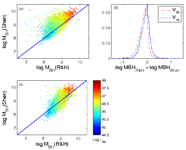
Figure 12: ${\rm Log}\textrm{{$\mathcal{M}_{\textrm{BH}}$}}(Shen)$ versus $\log\textrm{{$\mathcal{M}_{\textrm{BH}}$}}(R\&H)$ in solar units for two scenarios. (a) Before applying PCA and RPC. (c) After applying PCA and before RPC. Panel (b) shows that the Shen et al. (2008) masses are overall somewhat larger than ours; $M_{bb}$ and $M_{ab}$ are our $\mathcal{M}_{\textrm{BH}}$ values computed before and after applying PCA (but before applying RPC) respectively. The steeper slope in panel (c) is due to the same effect on $\sigma_{MgII}$ measurement as in Figure 11, meaning that relative to our masses, the high mass BHs are overestimated in Shen et al. (2008) while the low mass BHs are underestimated. See the online version for color Figures.

for $\chi^{2}_{\nu}\approx 1$ with an intrinsic scatter of $\sim 35\%$. Some of this intrinsic scatter arises because the luminosity measurements are not necessarily co-temporal with the time-lag measurements. However, quasar variability on timescales of 100 or more rest-frame days can be roughly described by a Gaussian with $\sigma_{m}=0.2$ magnitudes (Figure 12 of Vanden Berk et al. 2004). The corresponding additional scatter in the $\tau_{BLR}$-$\ell$ relationship should therefore be roughly described by a Gaussian with $\sigma=0.04$ dex, or about 10%.

McLure and Jarvis (2002) estimated a correlation for $R_{BLR}$ with luminosity at 3000Å by using the reverberation mapping data of 34 quasars from Wandel et al. (1999) and Kaspi et al. (2000) and found $R_{BLR}=(25.2\pm 3.0)\ell^{0.47\pm 0.05}$ where $R_{BLR}$ is in units of light days. Both of our correlations are well defined only for quasars with $0.1<z<0.5$ within the luminosity range $0.001<\ell<100$. However, we assume that our correlation will hold for objects with luminosity and redshift beyond those limits (as tentatively found for C iv by Kaspi et al. 2007, but see appendix A1 of McLure & Dunlop 2004 for a contrary result).

We can determine the average geometrical factor, $\bar{f}$, in Equation 1 through comparing our virial mass estimates with the reverberation mass estimates by Peterson et al. (2004), which are calibrated to the $\mathcal{M}_{\textrm{BH}}-\sigma_{\star}$ correlation as described in Onken et al. (2004). We assume a linear fit with a fixed zero intercept for the virial product, $VM_{BH}=R_{BLR}\sigma_{intr}^{2}/G$, versus reverberation black hole mass, $RM_{BH}$. (A fit where the intercept is allowed to vary yields an intercept consistent with zero at $\ll 1\sigma$). The reduced chi squared, $\chi^{2}_{\nu}$, is calculated from:

$$\chi^{2}_{\nu}=\frac{1}{N-1}\sum_{i=1}^{N}\frac{[(VM_{BH})_{i}\bar{f}-(RM_{BH})_{i}]^{2}}{\sigma_{VM}^{2}+\sigma_{RM_{BH}}^{2}+\epsilon_{0}^{2}}$$ (8)

where the geometrical factor - which is the slope of the linear fit - is $\bar{f}=5.3\pm 0.6$ with $\chi_{\nu}^{2}\simeq 1.92$ ($N=15$) considering an intrinsic scatter of $\epsilon_{0}\simeq 35\%$ for the estimated masses from both methods. The relationship between mass, luminosity and linewidth is:

$$\textrm{{$\mathcal{M}_{\textrm{BH}}$}}/\textrm{{$\mathcal{M}_{\odot}$}}=5.75\bar{f}\ell^{0.5}\sigma_{intr}^{2}\pm\sigma_{\textrm{{$\mathcal{M}_{\textrm{BH}}$}}/\textrm{{$\mathcal{M}_{\odot}$}}}(\textrm{statistical})$$

$$\pm 24\%(\textrm{systematic})$$

$$\pm 35\%(\textrm{intrinsic~{}scatter})$$ (9)

where the constant 5.75 is the conversion factor for using BH masses in solar units when $\ell=[\lambda L_{3000}/10^{44}]$ is in units of erg s^-1, and the intrinsic line dispersion of the Mg ii emission line, $\sigma_{intr}$, is in units of km s^-1. The statistical error of the black hole mass estimates, $\sigma_{\textrm{{$\mathcal{M}_{\textrm{BH}}$}}/\textrm{{$\mathcal{M}_{\odot}$}}}$, can be calculated from:

$$\sigma_{\textrm{{$\mathcal{M}_{\textrm{BH}}$}}/\textrm{{$\mathcal{M}_{\odot}$}}}=2.875[\frac{\sigma^{2}_{intr}\bar{f}^{2}}{\ell}(\sigma_{\ell}^{2}\sigma_{intr}^{2}+16\sigma_{\sigma_{intr}}^{2}\ell^{2})]^{0.5}.$$ (10)

where $\sigma_{\sigma_{intr}}$ and $\sigma_{\ell}$ are estimated errors from our fitting process. The scatter of 35% is equivalent to 0.15 dex.

The systematic error of 24% (equivalent to 0.10 dex) comes from propagating the relative errors of the geometrical factor $\bar{f}$ and of the coefficient in the $\tau_{BLR}-\ell$ relation (Equation 6). It does not include any uncertainty in the exponent of the $\tau_{BLR}-\ell$ relation.

4 The Sample

In this study we use using spectra from the SDSS Data Release Three (DR3; Abazajian et al. 2005). The SDSS wavelength coverage sets the upper and lower limits for our sample selection. A spectrum needs to have the rest-frame wavelength of 2192-3027 Å within the SDSS range, since we fit that region around the Mg ii emission line (2798 Å) with a power law continuum and Fe ii emission template.

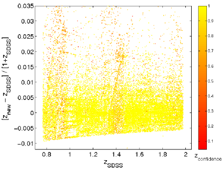
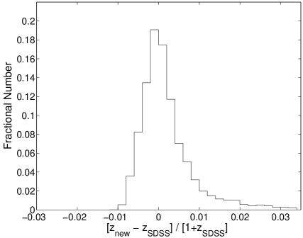
Figure 2: The top panel shows the relative change in quasar redshift after cross correlating the median quasar composite spectrum (Vanden Berk et al. 2001) with SDSS quasar spectra versus the SDSS redshift estimates described in §4.10.2.1 of Stoughton et al. (2002). The colormap is based on the estimated redshift confidence from the SDSS catalogue (Stoughton et al. 2002). The bottom panel shows the distribution of the relative change in quasar redshift. See the online version for color Figures.

The above condition defines our acceptable redshift range, which is $0.7336<z_{SDSS}<2.0393$. However, the redshift given in the DR3 quasar catalog (Schneider et al. 2005), as described in §4.10.2.1 of Stoughton et al. (2002), is not always as accurate as we need to place the Mg ii emission line sufficiently close to $2800$ Å in the adopted rest frame. Thus, we cross correlate the median quasar composite spectrum (Vanden Berk et al. 2001) with SDSS DR3 spectra (using the IRAF task ”xcsao”) to redefine the object’s redshift. These corrected redshift will be reliable only when relative change of the redshifts is smaller than $2\%$. Consequently the new redshift range will come from $|(z_{new}-z_{SDSS})|/(1+z_{SDSS})\simeq 2\%$. The top panel in Figure 2 shows the relative change in redshifts versus SDSS DR3 redshift, color-coded with the redshift confidence from the SDSS DR3 (Stoughton et al. 2002). Indeed, redshifts with lower confidence in SDSS DR3 tend to have larger redshift corrections. The bottom panel in Figure 2 shows the distribution of both redshift estimates.

These new redshift limits, $0.6996<z_{new}<2.1013$, however, include those objects where after redshift correction they have been shifted to the acceptable wavelength range (or maybe shifted out of the range), where the acceptable range is still defined by the normalization region.

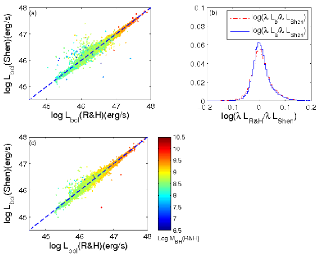
Figure 10: ${\rm Log}L_{bol}(Shen)$ versus $\log L_{bol}(R\&H)$ for two scenarios. (a) Before applying PCA and RPC. (c) After applying PCA and before RPC. $L_{b}$ and $L_{a}$ are Luminosities before and after applying PCA (but before applying RPC) respectively. Both panels show consistency between Shen et al. (2008) and this study; in both, there is a 0.1 dex scatter on the distribution (panel b) due to statistical errors. See the online version for color Figures.

The luminosities of our calibration objects come from total magnitudes, but SDSS DR3 spectra are scaled only to the flux in a 3″ diameter aperture. The average correction factor we apply to the flux measured from SDSS DR3 spectra to produce the total flux of all our objects is $-$0.35 magnitudes, which is appropriate for unresolved objects in the SDSS DR3 (see section 4.1.1 of Adelman-McCarthy et al. 2008). While this is an average correction, it is appropriate for quasars at all redshifts and luminosities in our sample ($z>0.7$ and $M_{i}<-24$), as the fraction of SDSS quasars with extended morphologies at those luminosities is at most 2% (Figure 10 of Vanden Berk et al. 2006).

Using our new quasar redshifts, the percentage of the successful fits in DR3 sample is about $79\%$ of the initially selected sample. To increase the fraction of acceptable fits and to reduce the noise we later use the eigenspectra method to reconstruct the quasar spectra (see section 5). This increases the percentage of acceptable fits to $94\%$. The remaining $6\%$ have problems such as a lack of data exactly at the Mg ii region, or a very broad absorption line very close to Mg ii or the normalization regions. In the end, our DR3 sample consists of 93.3% of all quasars with $0.7336<z_{SDSS}<2.0393$ (27602 quasars out of 29582).

Note that the objects in our catalogue are not homogeneously selected. However, of the 9325 quasars in redshift range in the homogeneous subsample of Richards et al. (2006), our DR3 sample contains 8814 (94.5%). Quasars in that complete subsample are flagged in the DR3 mass catalogue, and only such quasars should be used for studies that require a volume-limited, homogeneously selected sample. However, even in such studies the effects of Malmquist bias must be taken into account (see §8.2).

5 Reconstructing quasar spectra from quasar eigenspectra

Principal Component Analysis (PCA), sometimes called the Karhunen-Loève transformation, is an orthogonal linear transformation of data to a new coordinate system. As a result of this transformation the greatest variance by any projection of the data forms the first coordinate (called the first principal component or first eigenspectrum), the second greatest variance forms the second coordinate, and so on. Thus the great advantages of using PCA is that a number of possibly correlated variables transform into a smaller number of orthogonal variables called principal components.

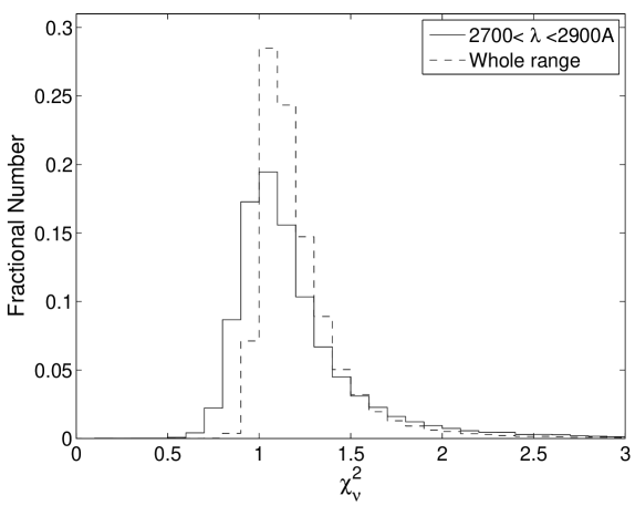
Figure 5: The distribution of the $\chi^{2}_{\nu}$ comparing the reconstructed spectra using PCA technique with raw spectra for two cases: solid curve compares within the window $2700$ Å$<\lambda<2900$ Å, dash-line curve compares the whole spectrum. See the online version for color Figures.

Yip et al. (2004) have applied this transformation to a sample of 16707 quasar spectra from the SDSS DR1 to generate such principal components. They have performed the transformation on subsamples with different redshift ($z$) and absolute magnitude ($M_{i}$) in the $i$ filter to generate eigenspectra for each ($M_{i},z$) bin. Using this technique they separate any possible luminosity effect on the spectra from any evolutionary effects. In each ($M_{i},z$) bin, the flux values from all quasars as a function of rest-frame wavelength are the data points on which the PCA is run. Therefore, PCA generates eigenspectra which span the same rest-frame wavelength range as the input spectra. Yip et al. (2004) show that the first four eigenspectra in each ($M_{i},z$) bin account for 82% of the total sample variance. These four eigenspectra represent the mean spectrum, a host-galaxy component, UV-optical continuum slope variations, and the correlations of Balmer emission lines respectively. We used all 50 eigenspectra calculated by Yip et al. (2004) in the appropriate ($M_{i}$,$z$) bin to provide the most accurate reconstruction of our spectra possible. We considered using only the number of eigenspectra needed to reach $\chi_{\nu}^{2}=1$ for each object, but such an approach is not possible for all objects with the Yip et al. (2004) eigenspectra because Figure 5 shows that most of our objects would require more than 50 eigenspectra to reach $\chi_{\nu}^{2}=1$.

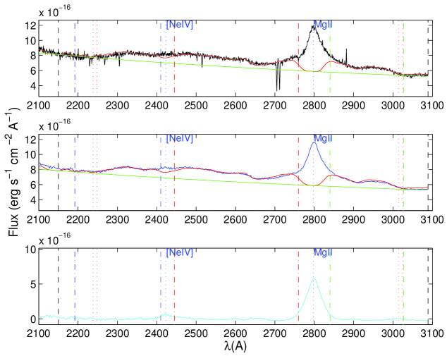
Figure 3: A sample SDSS quasar spectrum, before and after reconstruction using PCA, and our best pseudo-continuum estimates for it. The top panel shows the observed SDSS spectrum (black) and continuum (green) and the best pseudo-continuum fit (red). The middle panel shows the PCA reconstructed spectrum (blue) and continuum (green) and the best pseudo-continuum fit (red). The bottom panel shows the reconstructed spectrum in cyan after subtracting the best pseudo-continuum. The dotted red vertical lines show the normalization windows where we initially estimate the normalization of the power law, $2238-2248$ Å and $3014-3027$ Å. The dotted blue lines show two emission lines Mg ii and [Ne iv]. The dot-dashed lines determine the ranges within which we calculate the $\chi^{2}$ of the pseudo-continuum fit. The black dashed lines are the borders of the fitting region. Narrow absorption lines and noise spikes within the Fe ii fitting region have been removed through PCA reconstruction. See the online version for color Figures.

We have used the 50 most significant eigenspectra from Yip et al. (2004) (the luminosity, redshift dependent eigenspectra) to reproduce the spectrum of each quasar. The reproduced spectra have the same continua as the original spectra, and the most significant features like emission lines are the same. However, the reconstructed spectra have less noise as compared to the original spectra. Any narrow absorption lines are removed through this method, and narrow regions of missing data are effectively reconstituted by the best-fit reconstruction found for the rest of the spectrum. In Figure 3 we show an example of an SDSS quasar spectrum before and after PCA reconstruction. The top panel shows the raw spectrum and our best pseudo-continuum estimate for it, and the middle panel the same for the reconstructed spectrum. The bottom panel shows the decontaminated spectrum which we use to measure the Mg ii line dispersion.

In Figure 5 we show the distribution of the reduced $\chi^{2}$ calculated for DR3 catalogue by comparing reconstructed spectra and raw spectra for two cases: first, using a window around Mg ii between $2700$Å and $2900$Å and second, using the entire fitting region of 2192-3027Å. For both cases, the peak is located near unity, indicating that the PCA reconstructions are statistically acceptable fits to the original spectra.

6 Radiation Pressure Correction (RPC) on Scaling Relationship

The virial theorem can be used for a dynamically relaxed gravitationally bound system. However, very luminous sources can violate this assumption. In such sources, the gravitational force of a BH can be reduced by the effect of the radiation pressure (Marconi et al. 2008). If BLR clouds are attracted by a smaller effective force of gravity, their line dispersion decreases, resulting in mistakenly underestimated virial BH mass estimates. Therefore, the scaling relationships may therefore need to be recast to include the effect of radiation pressure.

We have applied the Marconi et al. (2008) suggestion to correct the scaling relationship for the Mg ii emission line such that $\textrm{{$\mathcal{M}_{\textrm{BH}}$}}/\textrm{{$\mathcal{M}_{\odot}$}}=5.75\bar{f}_{a}\ell^{0.5}\sigma_{intr}^{2}+\bar{g}\ell$ where $\ell=[\lambda L_{3000}/10^{44}]$erg s^-1and $\sigma_{intr}$ is the line dispersion of the Mg ii line in units of km s^-1. We use the same sample as in § 3 to determine the adjusted calibration factors, $\bar{f}_{a}$ and $\bar{g}$, through comparison of our virial mass estimates adjusted for radiation pressure with the black hole mass estimates $M_{BH}^{*}$ made directly from the black hole mass - bulge velocity dispersion relationship for quiescent galaxies (Equation 1 in Tremaine et al. 2002). We assume that the relationship holds for AGNs and their host galaxies too. The velocity dispersions $\sigma_{*}$ are extracted for 11 objects from Onken et al. (2004) and for two objects, PG1229+204 and PG2130+099, from Dasyra et al. (2007). We assume a non-linear fit with a variable intrinsic scatter for the Adjusted Virial Mass ($AVM_{BH}$) versus $M_{BH}^{*}$. The reduced chi squared, $\chi^{2}_{\nu}$, is calculated from:

$$\chi^{2}_{\nu}=\frac{1}{N-3}\sum_{i=1}^{N}\frac{[(AVM_{BH})_{i}-(M_{BH}^{*})_{i}]^{2}}{\sigma_{VM}^{2}+\sigma_{M_{BH}^{*}}^{2}+\epsilon_{0}^{2}}$$ (11)

Where the adjusted calibration factors are $\bar{f}_{a}=2.4\pm 1.5$ and $\log\bar{g}=6.9\pm 0.5$ with $\chi_{\nu}^{2}\simeq 1.00$ ($N=12$; after excluding 3C390.3) considering an intrinsic scatter of $\epsilon_{0}\simeq 15\%$. The adjusted mass scaling relation using Mg ii emission line is:

$$\textrm{{$\mathcal{M}_{\textrm{BH}}$}}/\textrm{{$\mathcal{M}_{\odot}$}}=5.75\bar{f}_{a}\ell^{0.5}\sigma_{intr}^{2}+\bar{g}\ell$$

$$\pm\sigma_{\textrm{{$\mathcal{M}_{\textrm{BH}}$}}/\textrm{{$\mathcal{M}_{\odot}$}}}(\textrm{statistical})$$

$$\pm 15\%(\textrm{intrinsic~{}scatter}).$$ (12)

The statistical error of the black hole mass estimates, $\sigma_{\textrm{{$\mathcal{M}_{\textrm{BH}}$}}/\textrm{{$\mathcal{M}_{\odot}$}}}$, can be calculated from:

$$\sigma_{\textrm{{$\mathcal{M}_{\textrm{BH}}$}}/\textrm{{$\mathcal{M}_{\odot}$}}}=[\sigma_{\ell}^{2}(2.875\frac{\bar{f}_{a}\sigma_{intr}^{2}}{\ell^{0.5}}+\bar{g})^{2}+132.2\sigma_{\sigma_{intr}}^{2}\sigma_{intr}^{2}{\bar{f}_{a}}^{2}\ell)]^{0.5}$$ (13)

where $\sigma_{\sigma_{intr}}$ and $\sigma_{\ell}$ are estimated errors from our fitting process. The scatter of 15% corresponds to less than 0.07 dex of intrinsic scatter. We do not quote a systematic error (which comes from the systematic errors on $\bar{f}_{a}$ and $\bar{g}$) because its magnitude depends on the relative values of the two terms in Equation 6, which will be different for objects of different luminosities and linewidths.

When the estimated line dispersion of Mg ii is very small then $\lim_{\sigma\rightarrow 0}\textrm{{$\mathcal{M}_{\textrm{BH}}$}}/\textrm{{$\mathcal{M}_{\odot}$}}=\bar{g}\ell$. Using our luminosity limits we have a lower limit on black hole mass estimates for the adjusted method of $\log(\frac{\textrm{{$\mathcal{M}_{\textrm{BH}}$}}}{\textrm{{$\mathcal{M}_{\odot}$}}})\gtrsim 6.9$ for $\lambda L_{3000}>10^{44}$ erg s^-1. Whether this is a real constraint remains an open question.

7 Noise Simulation

We now evaluate the statistical errors on BH mass estimates from reconstructed spectra due to the presence of different noise levels in quasar spectra before reconstruction. We select 100 quasars with the highest signal to noise ratio (SNR), from 20 to 50. Then we add randomly generated Gaussian noise to these spectra to decrease the SNR to 1/2, 1/4, 1/8, and 1/16 of the original SNR (see Figure 4). We repeat this process for each new SNR 6 more times to have at least 25 realizations for every spectrum, yielding 2500 spectra in total. We extract quantities like $\lambda~{}L_{3000}$ and $\sigma_{MgII}$ (see section 2.1 and 2.2) and for four different cases; before or after reconstructing the spectra by applying PCA and before or after applying the radiation pressure correction (RPC).

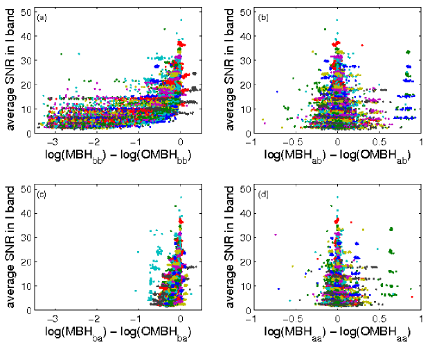
Figure 6: The log difference of the BH mass estimates for four scenarios. Different objects are represented in different colors. In all Figures, subscript a stands for after and subscript b stands for before. The first subscript states the PCA status while the second subscript states the Radiation Pressure Correction (RPC) status. Masses are estimated (a) before applying PCA and before RPC; (b) after applying PCA and before RPC; (c) before applying PCA but after RPC; (d) after applying PCA and after RPC. The cutoff on lower mass estimates in panel (c) is due to the asymptotic limit when $\sigma_{line}\rightarrow 0$. The presence of the light blue points at x-axis $\sim-0.7$ in this panel are due to the presence of the broad absorption line (BAL) in the Mg ii window of an object. See the online version for color Figures.

Figure 6 shows, as a function of the average SNR in the $I$ band, the differences in the logarithms of the black hole mass estimated after adding noise to spectra ($MBH$) and the mass estimated using original spectra with high SNR ($OMBH$) for four scenarios. As we can see from these Figures, the lower the SNR, the more the BH mass is uncertain with respect to the high SNR mass estimate. Comparing Figure 6a with Figure 6b shows an improvement in removing the systematic underestimation of BH masses when the spectra are reconstructed using PCA. Comparing Figure 6a with Figure 6c shows a cutoff on the lower side of the mass estimates in Figure 6c. This lower limit is due to the asymptote approached when the estimated line dispersion is very small ($\lim_{\sigma\rightarrow 0}\textrm{{$\mathcal{M}_{\textrm{BH}}$}}/\textrm{{$\mathcal{M}_{\odot}$}}=\bar{g}\ell$) in the scenario when the RPC is applied. There were also three objects out of 100 selected with high SNR for which the results are catastrophic. One object is not being reconstructed properly due to an error on the redshift estimate, and two objects have a broad absorption line right in the Mg ii window. Setting aside the 3% catastrophic errors, the scatter is normally distributed around zero when PCA reconstruction is applied (see, e.g., Figure 6b and 6d).

In Figure 6a, if there was no SNR dependency then we would expect a Gaussian distribution around zero. The negative trend in mass difference in low SNR level shows the high sensitivity of the method to the SNR. In Figure 6c, the non-symmetrical trend in low SNR emphasizes the SNR dependency too. This implies that using second moment of the line profile to estimate the $\sigma_{line}$ without PCA reconstruction is unbiased only for spectra with the very high SNR ($SNR>30$) while after PCA reconstruction there is no such systematic bias with the SNR, making the PCA reconstruction a necessary step in precise estimation of BH mass algorithm.

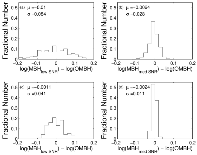
Figure 7: The distribution of the log difference of the BH mass estimates for two SNR bins: (a) and (c) $1.5<SNR_{I}<2.4$; (b) and (d) $18<SNR_{I}<23$. All plots are after applying PCA and for two scenarios: (a) and (b) before RPC; (c) and (d) after RPC. The mean ($\mu$) and the standard deviation ($\sigma$) of each distribution are reported in each panel. Comparing Figure (a) to (b) or comparing Figure (c) to (d) shows a factor of 3-3.7 improvement in mass estimates when high SNR is used. Comparing Figure (a) to (c) or comparing Figure (b) to (d) we have a factor of 2-2.5 improvement due using RPC.

Comparing the mass estimates from these different cases we can conclude that: using PCA improves the mass estimation scatter to better than 0.4 dex for SNR as low as 1.5 or to better than 0.2 dex for SNR of 18 (see Figures 7a and 7b). This improvement is due to the sensitivity of the Fe ii modeling process and the second moment measurement to both the SNR and the accuracy of the power-law estimates for quasar spectra. Using PCA along with considering the effect of the radiation pressure improves the mass estimation scatter to better than 0.2 dex for SNR of around 1.5 (see Figures 7c and 7d). Overall, BH mass estimates are around 50% less scattered for either high or low SNR if we consider the effect of the radiation pressure (compare Figure 6b to 6d). However, BH masses are around 3 to 4 times less scattered in the high SNR regime than in the low SNR regime, either before (Figure 6b) or after the radiation correction (Figure 6d), but only if we reconstruct the spectra.

Denney et al. (2009) have studied the effect of the SNR on reverberation BH mass estimates using both FWHM and line dispersion of quasar NGC 5548. They have reported a similar dependency on SNR as we see before reconstructing the spectra.

8 Catalogue and Results

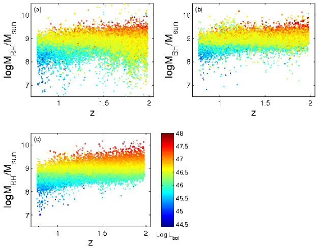
Figure 8: The $\log~{}\textrm{{$\mathcal{M}_{\textrm{BH}}$}}$ versus redshift plane for three scenarios. (a) Before applying PCA and RPC. (b) After applying PCA and before RPC. (c) After applying PCA and RPC. The lack of low mass BHs at high $z$ and high mass BHs at low $z$ is due to detection and saturation limits. BH masses between $10^{8.5}$ and $10^{9.3}$ are distributed all over our redshift range. See the online version for color Figures.

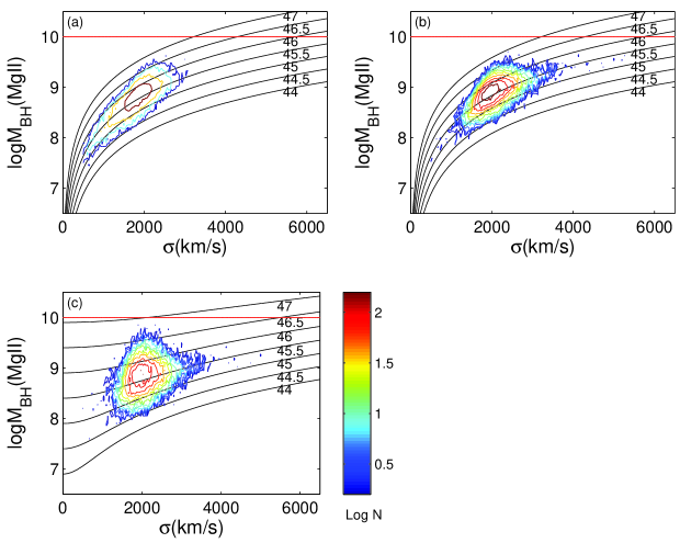
Figure 9: Contours of $\log~{}\textrm{{$\mathcal{M}_{\textrm{BH}}$}}$ in solar units versus $\sigma_{MgII}$ plane for three scenarios. (a) Before applying PCA and RPC. (b) After applying PCA and before RPC. (c) After applying PCA and RPC. The black curves show the $\log~{}\textrm{{$\mathcal{M}_{\textrm{BH}}$}}$ versus $\sigma_{MgII}$ for a fixed $\log~{}L_{bol}$ ranging from 44 to 47. The red line $\log~{}\textrm{{$\mathcal{M}_{\textrm{BH}}$}}=10$ represents the upper mass limit suggested by Shen et al. (2008). See the online version for color Figures.

Here we present a catalogue including black hole mass estimates for three scenarios: black hole masses before applying PCA and before RPC ($MBH_{bb}$; see, e.g., Figure 8a), BH masses after applying PCA but before RPC ($MBH_{ab}$; see, e.g., Figures 8b), and BH masses after applying PCA and after RPC ($MBH_{aa}$; see, e.g., Figures 8c). We present several quantities in this catalogue including the $\sigma_{MgII}$ and $\lambda~{}L_{3000}$ (see Table 3 for more information about the catalogue format). In Figures 8 and 9 we present plots of different quantities corresponding to these three different scenarios. Comparing panel (b) against panel (a) of these Figures represent the advantages of using PCA reconstruction while comparing panel (c) against panel (b) reveals the RPC.

The artificially low black hole mass estimates (especially in the high redshift regime) in Figure 8a are mostly removed after PCA reconstruction in Figure 8b and 8c. The masses were underestimated due to the decreased velocity range over which $\sigma_{line}$ could be reliably measured in low SNR spectra. Forcing $\sigma_{line}$ to be measured over a fixed velocity range regardless of SNR might reduce the mass underestimation in low-SNR unreconstructed spectra, but only at the cost of much larger scatter on $\sigma_{line}$. Figure 8b shows that very massive black holes ($\gtrsim 10^{9.3}M_{\odot}$; the red points in the color version) were active as quasars at $z\gtrsim 1.5$. However, a more reasonable true upper mass limit in our redshift range, considering the errors which broaden the mass distribution, is perhaps $10^{9.5}M_{\odot}$.

For first scientific uses of this catalogue, see the BH spin evolution study of Rafiee & Hall (2009) and the sub-Eddington boundary study of Rafiee & Hall (2011).

8.1 Comparing with Shen et al. 2008

Shen et al. (2008) have estimated black hole masses using the FWHMs of the Mg ii, H$\beta$ and C iv emission lines for objects in the SDSS DR5 quasar sample. We have extracted the FWHM Mg ii BH masses, $L_{bol}$, and the FWHM of the same objects in our DR3 catalogue from Shen at al. (2008).

Figure 10 (a and b) shows the relationship between our bolometric luminosity and that of Shen et al. (2008) for the same objects. There is a 0.1 dex scatter on the distribution of the log of the ratio of $\lambda L_{3000}$ measurements (panel b) which is due to statistical errors.

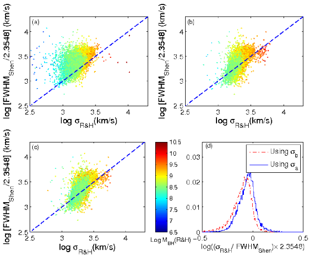
Figure 11: ${\rm Log}(\textrm{FWHM}_{Shen}/2.3548)$ versus $\log\sigma_{R\&H}$ for three scenarios. (a) Before applying PCA and RPC. (b) After applying PCA and before RPC. (c) After applying PCA and RPC. Although $\sigma_{a}$ (the line dispersion after applying PCA) is the same in both (b) and (c) they generate different $\mathcal{M}_{\textrm{BH}}$ distributions since the scaling relationship is different. $\sigma_{b}$ is the line dispersion before applying PCA. Panel (d) shows the distribution of the ratio of our measured line dispersion to the FWHM measured by Shen et al. (2008) in the same objects, relative to the value of 1/2.3548 expected for a Gaussian. See the online version for color Figures.

The Mg ii emission line width comparison shows a significant difference between our estimates and those of Shen et al. (2008) (see Figure 11, panels a to c). The larger scatter in Figure 11a is due to a systematic underestimate of $\sigma$ in unreconstructed low-SNR spectra. Figure 11d shows the distribution of the ratio of our measured line dispersion to the FWHM measured by Shen et al. (2008) in the same objects, relative to the value of 1/2.3548 expected for a Gaussian. At fixed FWHM, most quasar Mg ii emission lines have less flux in their wings than a Gaussian would.

Figure 12 compares our $\log M_{BH}$ estimates with those of Shen et al. (2008). Figure 12a illustrates the effect of the systematic underestimation of $M_{BH}$ in unreconstructed low-SNR spectra (Figure 6a). However, even in PCA-reconstructed spectra (Figure 12c) our BH mass estimates differ significantly from those of Shen et al. (2008). We note from Figure 6b that there are no systematic errors in our mass measurements from reconstructed spectra as a function of SNR; we therefore have confidence in our measurements. Figure 12b shows that the Shen et al. (2008) masses are overall somewhat larger than ours. Figure 12c illustrates that relative to our masses from PCA-reconstructed spectra, the Shen et al. (2008) masses are, on average, overestimated at higher masses and underestimated at lower masses.

The Mg ii emission line width comparison shows a significant difference between our estimates and those of Shen et al. (2008) (see Figures 11a to 11c). However, we note from Figure 6b that there is no systematic errors in our mass measurements as a function of SNR.

8.2 Malmquist Bias and the true distribution of BH masses

A Malmquist bias ($\delta_{M}$; Eddington 1913; Malmquist 1922), i.e., the difference between the mean values of the distributions of the true BH masses and the observed BH masses, is estimated for each of our three scenarios. This Malmquist bias, which is a selection effect, exists since we are using a flux-limited sample of quasars and since the mass function of quasars is very steep. There are more quasars with small masses being scattered to large masses in our sample by random uncertainties than there are quasars with large masses being scattered to small masses in our sample, leading to overestimated BH masses on average.

We use the generalized idea of the bias at fixed observed luminosity described in detail by Shen et al. (2008). This bias is estimated as $\delta_{M}=-\gamma_{M}\sigma_{\Upsilon}^{2}\textrm{ln}(10)/(1+C_{2})^{2}$ where $C_{2}$ is the slope of the assumed relationship between $\log\textrm{{$\mathcal{M}_{\textrm{BH}}$}}_{,true}$ and $\langle\log\Upsilon\rangle$, where $\Upsilon=L_{bol}/L_{Edd}$ is the Eddington ratio and $\gamma_{M}$ is the slope when we assume a power-law distribution for the underlying true BH masses as $N(\textrm{{$\mathcal{M}_{\textrm{BH}}$}})\propto\textrm{{$\mathcal{M}_{\textrm{BH}}$}}^{\gamma_{M}}$. The $\sigma_{\Upsilon}$ is defined as the dispersion of the true distribution of the Eddington ratio (see Shen et al. 2008 for more details). Shen et al. has modeled the underlying distribution of the true BH masses and estimated $C_{2}=0.3$ and $\gamma_{M}=-2.6$ for the redshift bin of $0.7<z<1.0$. We assume the same distribution of true BH masses and estimate the $\sigma_{\Upsilon}$ for all three of our scenarios. We then estimate the Malmquist bias ($\delta_{M}$) of the three scenarios to be $\delta_{M}(bb)\simeq 0.44$, $\delta_{M}(ab)\simeq 0.40$, and $\delta_{M}(aa)\simeq 0.11$. However, we do not apply these estimated Malmquist biases on reported BH masses in the catalogue, as the calculation of the Malmquist bias is model dependent and users of the catalogue may wish to apply a differently calculated correction. The Malmquist bias for the case after applying both PCA and RPC is very small since the BH mass distribution is dominated by the narrow distribution of the luminosity due to the radiation pressure correction (see Equation 6).

9 Conclusions

We have measured virial BH masses and radiation pressure adjusted virial BH masses for 27,602 quasars at $0.7<z<2.0$ in the SDSS DR3 quasar catalogue, and have made our mass estimates available to the community. We have used the second moment of the Mg ii emission line profile to estimate the line width and have calibrated a virial mass estimator using it and the monochromatic luminosity at 3000Å. The virial BH masses are typically in the range $10^{8}-10^{9.5}\textrm{{$\mathcal{M}_{\odot}$}}$ for our quasar sample (Figures 8 and 9).

We have reconstructed the quasar spectra using Principal Component Analysis to increase the number of quasars for which reliable masses can be measured and to eliminate systematic biases due to the presence of noise. We have tested the reliability and biases of the mass measurements as a function of SNR before and after this PCA reconstruction. Our noise simulation shows no systematic bias in measured BH masses as a function of SNR (section 7). Using PCA reconstructed spectra for measuring BH masses reduces the intrinsic scatter in the BH mass estimates.

For a subsample of Shen et al. (2008) quasars in common with our sample, we have compared the estimated bolometric luminosity, the line width, and the BH mass. The bolometric luminosities are mutually consistent, with 0.1 dex statistical scatter. However, with respect to this study, Shen et al. (2008) have overestimated the line width in the case of the broadest emission lines and underestimated the line width in the case of the narrowest emission lines. This difference in line width measurement has affected the BH mass estimates such that those of the most massive BHs in Shen et al. are overestimated and those of the least massive BHs are underestimated with respect to this study. We believe our black hole mass estimates are accurate. Improved understanding of black hole masses is necessary for understanding properties of the distribution of quasars in parameter space, such as the sub-Eddington boundary (Steinhardt & Elvis 2010; Rafiee & Hall 2011).

Figure 4: A typical quasar spectrum with noise added to produce spectra with different SNR levels (cyan). The spectrum reconstructed in each case using the 50 most significant PCA eigenspectra from Yip et al. (2004) is overplotted. (a) Reconstructed spectrum shown in black generated from spectrum with original SNR in cyan. (b) Reconstructed spectrum in blue generated from spectrum with $1/2$ original SNR. (c) Reconstructed spectrum in red generated from spectrum with $1/4$ original SNR. (d) Reconstructed spectrum in green generated from spectrum with $1/8$ original SNR. (e) Reconstructed spectrum in magenta from spectrum with $1/16$ original SNR. (f) over-plotting the 5 reconstructed spectra in panel (a) to (e). See the online version for color Figures.

Table 1: Calibration Data.

Object	DataID	$\sigma_{MgII}$	$\lambda L_{3000}/10^{44}$	$<\tau>_{H\alpha,\beta,\gamma}$	$M_{BH}$	flag 1	Virial $M_{BH}$	flag 2	Adjusted Virial $M_{BH}$	$\sigma^{*}_{bulge}$
		km/s	erg/s	days	$M_{\odot}\times 10^{6}$		$M_{\odot}\times 10^{6}$		$M_{\odot}\times 10^{6}$	km/s
1	2	3	4	5	6	7	8	9	10	11
3C120	LWP04500
	LWR16609
		3384.0	1.7472	38.10 ${}^{+21.30}_{-15.30}$	55.5 ${}^{+31.4}_{-22.5}$	-1	87.0 $\pm$ 3.7	1	222 $\pm$ 10	162.0 $\pm$ 24.0
3C390.3	LWP16776
	LWP03808
	LWP17245
	LWP18382
	LWP17259
	LWP17478
		19533.8	0.5397	23.60 ${}^{+4.38}_{-4.74}$	287.0 ${}^{+64.0}_{-64.0}$	-1	1610 $\pm$ 220	-1	3870 $\pm$ 540	240.0 $\pm$ 36.0
Akn120(Ark120)	Y29E0106T	1377.7	0.0417	39.05 ${}^{+4.16}_{-4.95}$	150.0 ${}^{+19.0}_{-19.0}$	1	2.2 $\pm$ 4.0	1	5.7 $\pm$ 11	239.0 $\pm$ 36.0
Fairall9	LWP24094
	LWP24095
	LWP06492
	LWP19270
	LWP19554
	LWP21475
	LWP21474
	LWP21473
	LWP19915
		1797.7	3.4198	17.40 ${}^{+3.20}_{-4.30}$	255.0 ${}^{+56.0}_{-56.0}$	1	34.4 $\pm$ 0.8	-1	109.6 $\pm$ 3.0	$\cdots$
Mrk110	LWP12760
	LWP12761
		1431.5	0.5864	24.37 ${}^{+4.63}_{-4.49}$	25.1 ${}^{+6.1}_{-6.1}$	1	9.0 $\pm$ 1.2	1	26.3 $\pm$ 4.0	86.0 $\pm$ 13.0
Mrk335	LWR11470
	LWR03512
	LWR09917
	LWR11947
	LWR14554
	LWR14555
	LWP19466
	LWP19123
	LWP16819
		2028.7	1.3369	15.27 ${}^{+3.88}_{-3.34}$	14.2 ${}^{+3.7}_{-3.7}$	1	27.4 $\pm$ 1.5	-1	76.3 $\pm$ 4.9	$\cdots$
Mrk509	LWR13716
	LWR01636
	LWP14218
	LWR01309
	LWP14534
	LWP10829
	LWP15474
	LWR06219
	LWP18844
	LWP18786
	LWP18785
		1977.1	4.1095	79.60 ${}^{+6.10}_{-5.40}$	143.0 ${}^{+12.0}_{-12.0}$	1	45.6 $\pm$ 0.8	-1	142.0 $\pm$ 3.2	$\cdots$
Mrk590	LWP19577
	LWR13721
		2246.2	0.7761	24.23 ${}^{+2.16}_{-2.01}$	47.5 ${}^{+7.4}_{-7.4}$	1	25.6 $\pm$ 2.5	1	67.5 $\pm$ 7.1	194.0 $\pm$ 20.0
Mrk79	LWR06141
	LWR01320
		1621.4	0.4975	14.38 ${}^{+4.02}_{-3.80}$	52.4 ${}^{+14.4}_{-14.4}$	1	10.7 $\pm$ 1.6	1	29.5 $\pm$ 5.0	130.0 $\pm$ 20.0
Mrk817	LWR11936	2054.0	1.0361	19.05 ${}^{+2.48}_{-2.41}$	49.4 ${}^{+7.7}_{-7.7}$	1	24.7 $\pm$ 1.8	1	67.5 $\pm$ 5.5	142.0 $\pm$ 21.0
NGC3783	LWP23003
	LWP23318
	LWP23311
	LWP23298
	LWP23289
	LWP23280
	LWP23094
	LWP23075
	LWP23073
	LWP23035
	LWP22902
	LWP22876
	LWP22845
	LWP22827
	LWP22826
	LWP23074
		1202.7	0.2696	10.20 ${}^{+3.30}_{-2.30}$	29.8 ${}^{+5.4}_{-5.4}$	1	4.3 $\pm$ 1.2	1	12.5 $\pm$ 4.1	95.0 $\pm$ 10.0
NGC4051	LWP23153
	LWP19265
	LWP27298
	LWP27297
	LWP24347
	LWP11100
		1131.4	0.0080	5.80 ${}^{+2.60}_{-1.80}$	1.9 ${}^{+0.78}_{-0.78}$	-1	0.7 $\pm$ 6.2	1	1.6 $\pm$ 16.0	84.0 $\pm$ 9.0
NGC5548	LWP24683
	LWP25088
	LWP25452
	LWP25440
	LWP25409
	LWP25464
	LWP25422
	LWP25483
	LWP25522
	LWP25514
	LWP25496
		1971.3	0.3769	16.81 ${}^{+0.97}_{-0.98}$	67.1 ${}^{+2.6}_{-2.6}$	1	13.7 $\pm$ 2.7	1	35.9 $\pm$ 7.7	183.0 $\pm$ 27.0
NGC7469	Y3B4010CT	1798.8	0.5957	4.54 ${}^{+0.64}_{-0.68}$	12.2 ${}^{+1.4}_{-1.4}$	1	14.4 $\pm$ 1.8	1	39.2 $\pm$ 5.5	152.0 $\pm$ 16.0
PG0844+349	LWP12206	1047.1	4.6751	31.99 ${}^{+13.45}_{-12.64}$	92.4 ${}^{+38.1}_{-38.1}$	-1	13.6 $\pm$ 0.2	-1	69.9 $\pm$ 1.7	$\cdots$
PG1211+143	LWP13628
	LWP07603
	LWP07223
	LWP23329
	LWP19386
		958.4	8.8465	103.94 ${}^{+17.39}_{-23.64}$	146.0 ${}^{+44.0}_{-44.0}$	1	15.7 $\pm$ 0.1	-1	108.0 $\pm$ 1.5	$\cdots$
PG1226+023	Y0G4020FT	1816.2	85.9274	352.99 ${}^{+32.10}_{-37.45}$	886.0 ${}^{+187.0}_{-187.0}$	1	175.8 $\pm$ 0.2	-1	1104 $\pm$ 1.6	$\cdots$
PG1229+204	LWR13136
	LWR16071
		1558.2	3.1430	33.33 ${}^{+14.59}_{-12.35}$	73.2 ${}^{+35.2}_{-35.2}$	-1	24.8 $\pm$ 0.6	1	84.4 $\pm$ 2.6	162.0 $\pm$ 32.0
PG1351+640	Y0P80305T
	O65616010
		1995.4	6.9307	$\cdots$	$\cdots$	-1	60.3 $\pm$ 0.7	-1	199.7 $\pm$ 2.8	$\cdots$
PG1411+442	Y11U0103T	1700.3	3.9038	101.58 ${}^{+31.00}_{-28.06}$	443.0 ${}^{+146.0}_{-146.0}$	1	32.8 $\pm$ 0.6	-1	109.8 $\pm$ 2.7	$\cdots$
PG2130+099	LWR04610
	LWP03568
		1478.9	3.9699	177.22 ${}^{+19.94}_{-12.68}$	457.0 ${}^{+55.0}_{-55.0}$	1	25.1 $\pm$ 0.5	1	91.7 $\pm$ 2.3	172.0 $\pm$ 46.0

Note. — Column 1 details the name of the objects and its resources. Column 2 are the IUE or HST spectra. Columns 3 and 4 are the Mg ii line dispersion in units of km s^-1 and the monochromatic luminosity at 3000Å respectively. Column 5 is the average time-lag in units of light-days from Peterson et al. 2004. Column 6 is the reverberation mapping BH mass estimates from Peterson et al. 2004. Columns 8 and 10 are the BH mass estimates for two scenarios, before or after applying the radiation correction, respectively. Columns 7 and 9 are the outlier flag in regression analysis; flag 1 for Virial $M_{BH}$ and flag 2 for Adjusted Virial $M_{BH}$. Column 11 is the stellar velocity dispersion of the bulge from Onken et al. 2004 and Dasyra et al. 2007.

Table 2: $\log(\tau)=\alpha\log(\ell)+\beta$, Fitting Results.

Fitting Method	Slope($\alpha$)	Intercept($\beta$)	Scatter
FITEXY	0.55 $\pm$ 0.02	1.49 $\pm$ 0.02	0
FITEXY	0.47 $\pm$ 0.12	1.46 $\pm$ 0.09	0.35
BCES(Y$|$X)	0.48 $\pm$ 0.16	1.46 $\pm$ 0.10	0
bootstrap	0.51 $\pm$ 0.20	1.43 $\pm$ 0.10	0
BCES Bisector	0.63 $\pm$ 0.11	1.44 $\pm$ 0.10	0
bootstrap	0.66 $\pm$ 0.18	1.43 $\pm$ 0.11	0
MCMC	0.40 $\pm$ 0.10	1.46 $\pm$ 0.08	0.33

Table 3: Catalogue Format.

Col	Format	Units	Label	Description
1	A18	$\cdots$	Name	SDSS J
2	F11.6	deg	RAdeg	Right Ascension in decimal degrees (J2000)
3	F11.6	deg	DEdeg	Declination in decimal degrees (J2000)
4	F7.5	$\cdots$	z	redshift
5	F7.4	$\cdots$	imag	PSF i-band apparent magnitude
6	F7.4	$\cdots$	iMag	PSF i-band absolute magnitude,K-corrected to z=2
7	I6	d	MJD	Modified Julian Date
8	I5	$\cdots$	Plate	Plate number
9	I5	$\cdots$	Fiber	Fiber identification number
10	F7.4	Å	si	Instrumental sigma
				Before applying PCA(2) and RPC(2)
11	F7.4	Å	sim_b	$\sigma_{MgII}$ estimates from the second moments
12	F7.4	Å	st_b	true $\sigma_{MgII}$ in Å
13	F9.6	erg s-1 cm-2 Å-1	F3_b	$F_{\lambda}$ at 3000 Å
14	F7.4	erg s-1	LL_b	Monochromatic luminosity at 3000Å, $\lambda L_{\lambda}$ in units 1E44 (4)
15	F8.4	light-days	R_ld_b	Radius of the BLR
16	F8.3	$\cdots$	SN_G_b	Median SNR in G band
17	F8.3	$\cdots$	SN_R_b	Median SNR in R band
18	F8.3	$\cdots$	SN_I_b	Median SNR in I band
19	F7.4	$M_{\odot}$	MBH_bb	BH mass in solar units
20	F7.4	$M_{\odot}$	Err_MBH_bb	Error in BH mass
				After applying PCA(2) but before RPC(2)
21	F7.4	Å	sim_a	$\sigma_{MgII}$ estimates from the second moments(3)
22	F7.4	Å	st_a	true $\sigma_{MgII}$ in Å (3)
23	F9.6	erg s-1 cm-2 Å-1	F3_a	$F_{\lambda}$ at 3000 Å (3)
24	F7.4	erg s-1	LL_a	Monochromatic luminosity at 3000Å, $\lambda L_{\lambda}$ in units of 1E44 (3)(4)
25	F8.4	light-days	R_ld_a	Radius of the BLR(3)
26	F8.3	$\cdots$	SN_G_a	Median SNR in G band
27	F8.3	$\cdots$	SN_R_a	Median SNR in R band
28	F8.3	$\cdots$	SN_I_a	Median SNR in I band
29	F7.4	$M_{\odot}$	MBH_ab	BH mass in solar units (3)
30	F7.4	$M_{\odot}$	Err_MBH_ab	Error in BH mass (3)
				After applying PCA(2) and RPC(2)
31	F7.4	$M_{\odot}$	MBH_aa	BH mass in solar units
32	F7.4	$M_{\odot}$	Err_MBH_aa	Error in BH mass
33	F7.4	$\cdots$	z_RH	redshift re-estimated by this study
34	I1	$\cdots$	DR3c	In DR3 complete subsample? (0=no, 1=yes)

Note. — (1) Entries reading 0.0000 or 0.0000e+00 indicate that the quantity was not measurable. (2) PCA stands for Principal Component Analysis and RPC stands for Radiation Pressure Correction. (3) Recommended results. (4) Bolometric Luminosity can be estimated using $BC(3000{\AA})$ = 5.15 and the monochromatic luminosity at 3000Å (Shen et al. 2008). Until the catalogue is available through the ApJS website it can be downloaded as http://ara.phys.yorku.ca/rafieehall2011.txt

References

- Abazajian et al. (2005) Abazajian, K., et al. 2005, AJ, 129, 1755
- Adelman-McCarthy et al. (2008) Adelman-McCarthy, J. K., et al. 2008, ApJS, 175, 297
- Akritas & Bershady (1996) Akritas, M. G., & Bershady, M. A. 1996, ApJ, 470, 706
- Bentz et al. (2006) Bentz, M. C., Peterson, B. M., Pogge, R. W., Vestergaard, M., & Onken, C. A. 2006, ApJ, 644, 133
- Bentz et al. (2009) Bentz, M. C., et al. 2009, ApJ, 705, 199
- Blandford & McKee (1982) Blandford, R. D., & McKee, C. F. 1982, ApJ, 255, 419
- Boroson & Green (1992) Boroson, T. A., & Green, R. F. 1992, ApJS, 80, 109
- Boroson & Lauer (2010) Boroson, T. A., & Lauer, T. R. 2010, arXiv:1005.0028
- Bruhweiler & Verner (2008) Bruhweiler, F., & Verner, E. 2008, ApJ, 675, 83
- Collin et al. (2006) Collin, S., Kawaguchi, T., Peterson, B. M., & Vestergaard, M. 2006, A&A, 456, 75
- Connolly et al. (1995) Connolly, A. J., Szalay, A. S., Bershady, M. A., Kinney, A. L., & Calzetti, D. 1995, AJ, 110, 1071
- Dasyra et al. (2007) Dasyra, K. M., et al. 2007, ApJ, 657, 102
- Denney et al. (2009) Denney, K. D., Peterson, B. M., Dietrich, M., Vestergaard, M., & Bentz, M. C. 2009, ApJ, 692, 246
- Done & Krolik (1996) Done, C., & Krolik, J. H. 1996, ApJ, 463, 144
- Eddington (1913) Eddington, A. S. 1913, MNRAS, 73, 359
- Ferrarese & Merritt (2000) Ferrarese, L., & Merritt, D. 2000, ApJ, 539, L9
- Gebhardt et al. (2000) Gebhardt, K., et al. 2000, ApJ, 539, L13
- Horne et al. (2004) Horne, K., Peterson, B. M., Collier, S. J., & Netzer, H. 2004, PASP, 116, 465
- Kaspi et al. (2005) Kaspi, S., Maoz, D., Netzer, H., Peterson, B. M., Vestergaard, M., & Jannuzi, B. T. 2005, ApJ, 629, 61
- Kaspi et al. (2000) Kaspi, S., Smith, P. S., Netzer, H., Maoz, D., Jannuzi, B. T., & Giveon, U. 2000, ApJ, 533, 631
- Kollatschny (2003) Kollatschny, W. 2003, A&A, 407, 461
- Kollatschny (2002) Kollatschny, W. 2002, Mass Outflow in Active Galactic Nuclei: New Perspectives, 255, 271
- Koratkar & Gaskell (1991) Koratkar, A. P., & Gaskell, C. M. 1991, ApJ, 370, L61
- Kormendy & Richstone (1995) Kormendy, J., & Richstone, D. 1995, ARA&A, 33, 581
- Krolik (2001) Krolik, J. H. 2001, ApJ, 551, 72
- Leighly (2000) Leighly, K. M. 2000, New Astronomy Review, 44, 395
- Lynden-Bell (1969) Lynden-Bell, D. 1969, Nature, 223, 690
- Marconi et al. (2008) Marconi, A., Axon, D. J., Maiolino, R., Nagao, T., Pastorini, G., Pietrini, P., Robinson, A., & Torricelli, G. 2008, ApJ, 678, 693
- McLure & Jarvis (2002) McLure, R. J., & Jarvis, M. J. 2002, MNRAS, 337, 109
- McLure & Dunlop (2004) McLure, R. J., & Dunlop, J. S. 2004, MNRAS, 352, 1390
- Miyoshi et al. (1995) Miyoshi, M., Moran, J., Herrnstein, J., Greenhill, L., Nakai, N., Diamond, P., & Inoue, M. 1995, Nature, 373, 127
- Netzer & Elitzur (1993) Netzer, N., & Elitzur, M. 1993, ApJ, 410, 701
- Onken et al. (2004) Onken, C. A., Ferrarese, L., Merritt, D., Peterson, B. M., Pogge, R. W., Vestergaard, M., & Wandel, A. 2004, ApJ, 615, 645
- Onken & Kollmeier (2008) Onken, C. A., & Kollmeier, J. A. 2008, ApJ, 689, L13
- Onken & Peterson (2002) Onken, C. A., & Peterson, B. M. 2002, ApJ, 572, 746
- Peterson (2007) Peterson, B. M. 2007, The Central Engine of Active Galactic Nuclei, 373, 3
- Peterson & Horne (2004) Peterson, B. M., & Horne, K. 2004, Astronomische Nachrichten, 325, 248
- Peterson (1993) Peterson, B. M. 1993, PASP, 105, 247
- Peterson & Wandel (2000) Peterson, B. M., & Wandel, A. 2000, ApJ, 540, L13
- Peterson & Wandel (1999) Peterson, B. M., & Wandel, A. 1999, ApJ, 521, L95
- Press et al. (1992) Press, W. H., Teukolsky, S. A., Vetterling, W. T., & Flannery, B. P. 1992, Numerical Recipes in FORTRAN, Cambridge: University Press, 2nd ed.
- Rafiee & Hall (2009) Rafiee, A., & Hall, P. B. 2009, ApJ, 691, 426
- Rafiee & Hall (2011) Rafiee, A., & Hall, P. B. 2011, MNRAS, submitted (arXiv:1011.1268)
- Richards et al. (2006) Richards, G. T., et al. 2006, AJ, 131, 2766
- Richstone et al. (1998) Richstone, D., et al. 1998, Nature, 395, A14
- Salpeter (1964) Salpeter, E. E. 1964, ApJ, 140, 796
- Schneider et al. (2005) Schneider, D., et al. 2005, AJ, 130, 367
- Schneider et al. (2010) Schneider, D., et al. 2010, AJ, 139, 2360
- Shen et al. (2008) Shen, Y., Greene, J. E., Strauss, M. A., Richards, G. T., & Schneider, D. P. 2008, ApJ, 680, 169
- Spergel et al. (2007) Spergel, D. N., et al. 2007, ApJS, 170, 377
- Steinhardt & Elvis (2010) Steinhardt, C. L., & Elvis, M. 2010, MNRAS, 402, 2637
- Stoughton et al. (2002) Stoughton, C., et al. 2002, Bulletin of the American Astronomical Society, 34, 1288
- Stoughton et al. (2002) Stoughton, C., et al. 2002, Proc. SPIE, 4836, 339
- Sulentic et al. (2000) Sulentic, J. W., Zwitter, T., Marziani, P., & Dultzin-Hacyan, D. 2000, ApJ, 536, L5
- Tremaine et al. (2002) Tremaine, S., et al. 2002, ApJ, 574, 740
- Tsuzuki et al. (2006) Tsuzuki, Y., Kawara, K., Yoshii, Y., Oyabu, S., Tanabé, T., & Matsuoka, Y. 2006, ApJ, 650, 57
- Ulrich & Horne (1996) Ulrich, M.-H., & Horne, K. 1996, MNRAS, 283, 748
- Vanden Berk et al. (2001) Vanden Berk, D. E., et al. 2001, AJ, 122, 549
- Vanden Berk et al. (2004) Vanden Berk, D. E., et al. 2004, ApJ, 601, 692
- Vanden Berk et al. (2006) Vanden Berk, D. E., et al. 2006, AJ, 131, 84
- Vestergaard (2009) Vestergaard, M. 2009, arXiv:0904.2615
- Vestergaard (2002) Vestergaard, M. 2002, ApJ, 571, 733
- Vestergaard & Wilkes (2001) Vestergaard, M., & Wilkes, B. J. 2001, ApJS, 134, 1
- Vestergaard & Peterson (2006) Vestergaard, M., & Peterson, B. M. 2006, ApJ, 641, 689
- Wandel et al. (1999) Wandel, A., Peterson, B. M., & Malkan, M. A. 1999, ApJ, 526, 579
- Wang et al. (2009) Wang, J.-G., et al. 2009, ApJ, 707, 1334
- Woo & Urry (2002) Woo, J.-H., & Urry, C. M. 2002, Bulletin of the American Astronomical Society, 34, 1109
- Woo & Urry (2002) Woo, J.-H., & Urry, C. M. 2002, ApJ, 579, 530
- Yip et al. (2004) Yip, C. W., et al. 2004, AJ, 128, 2603
- Yuan et al. (2004) Yuan, Q., Brotherton, M., Green, R. F., & Kriss, G. A. 2004, Recycling Intergalactic and Interstellar Matter, 217, 364
- Zel’Dovich & Novikov (1964) Zel’Dovich, Y. B., & Novikov, I. D. 1964, Soviet Physics Doklady, 9, 246