Linear Stationary Iterative Methods for the Force-based Quasicontinuum Approximation
Abstract.
Force-based multiphysics coupling methods have become popular since they provide a simple and efficient coupling mechanism, avoiding the difficulties in formulating and implementing a consistent coupling energy. They are also the only known pointwise consistent methods for coupling a general atomistic model to a finite element continuum model. However, the development of efficient and reliable iterative solution methods for the force-based approximation presents a challenge due to the non-symmetric and indefinite structure of the linearized force-based quasicontinuum approximation, as well as to its unusual stability properties. In this paper, we present rigorous numerical analysis and computational experiments to systematically study the stability and convergence rate for a variety of linear stationary iterative methods.
Key words and phrases:
atomistic-to-continuum coupling, quasicontinuum method, iterative methods, stability2000 Mathematics Subject Classification:
65Z05,70C201. Introduction
Low energy local minima of crystalline atomistic systems are characterized by highly localized defects such as vacancies, interstitials, dislocations, cracks, and grain boundaries separated by large regions where the atoms are slightly deformed from a lattice structure. The goal of atomistic-to-continuum coupling methods [22, 16, 1, 3, 4, 15, 28, 2, 26, 32] is to approximate a fully atomistic model by maintaining the accuracy of the atomistic model in small neighbors surrounding the localized defects and using the efficiency of continuum coarse-grained models in the vast regions that are only mildly deformed from a lattice structure.
Force-based atomistic-to-continuum methods decompose a computational reference lattice into an atomistic region and a continuum region , and assign forces to representative atoms according to the region they are located in. In the quasicontinuum method, the representative atoms are all atoms in the atomistic region and the nodes of a finite element approximation in the continuum region. The force-based approximation is thus given by [5, 6, 32, 10, 12, 11]
where denotes the positions of the representative atoms which are indexed by denotes the atomistic force at representative atom and denotes a continuum force at representative atom
The force-based quasicontinuum method (QCF) uses a Cauchy-Born strain energy density for the continuum model to achieve a patch test consistent approximation [6, 24, 11]. We recall that a patch test consistent atomistic-to-continuum approximation exactly reproduces the zero net forces of uniformly strained lattices [19, 24, 27]. However, the recently discovered unusual stability properties of the linearized force-based quasicontinuum (QCF) approximation, especially its indefiniteness, present a challenge to the development of efficient and reliable iterative methods [12]. Energy-based quasicontinuum approximations have many attractive features such as more reliable solution methods, but practical patch test consistent, energy-based quasicontinuum approximations have yet to be developed for most problems of physical interest, such as three-dimensional problems with many-body interaction potentials [21, 20, 30].
Rather than attempt an analysis of linear stationary methods for the full nonlinear system, in this paper we restrict our focus to the linearization of a one-dimensional model problem about the uniform deformation and consider linear stationary methods of the form
| (1) |
where is a nonsingular preconditioning operator, the damping parameter is fixed throughout the iteration (that is, stationary), and the residual is defined as
We will see below that our analysis of this simple model problem already allows us to observe many interesting and crucial features of the various methods. For example, we can distinguish which iterative methods converge up to the critical strain (see (8) for a discussion of the critical strain), and we obtain first results on their convergence rates.
We begin in Sections 2 and 3 by introducing the most important quasicontinuum approximations and outlining their stability properties, which are mostly straightforward generalizations of results from [11, 10, 9, 13]. In Section 4, we review the basic properties of linear stationary iterative methods.
In Section 5, we give an analysis of the Richardson Iteration () and prove a contraction rate of order in the norm (discrete Sobolev norms are defined in Section 2.1), where is the size of the atomistic system.
In Section 6, we consider the iterative solution with preconditioner where is a standard second order elliptic operator, and show that the preconditioned iteration with an appropriately chosen damping parameter is a contraction up to the critical strain only in among the common discrete Sobolev spaces. We show, however, that a rate of contraction in independent of can be achieved with the elliptic preconditioner and an appropriate choice of the damping parameter
In Section 7, we consider the popular ghost force correction iteration (GFC) which is given by the preconditioner and we show that the GFC iteration ceases to be a contraction for any norm at strains less than the critical strain. This result and others presented in Section 7 imply that the GFC iteration might not always reliably reproduce the stability of the atomistic system [9]. We did not find that the GFC method predicted an instability at a reduced strain in our benchmark tests [18] (see also [24]). To explain this, we note that our 1D analysis in this paper can be considered a good model for cleavage fracture, but not for the slip instabilities studied in [18, 24]. We are currently attempting to develop a 2D benchmark test for cleavage fracture to study the stability of the GFC method.
2. The QC Approximations and Their Stability
We give a review of the prototype QC approximations and their stability properties in this section. The reader can find more details in [10, 9].
2.1. Function Spaces and Norms
We consider a one-dimensional atomistic chain whose atoms have the reference positions for The displacement of the boundary atoms will be constrained, so the space of admissible displacements will be given by the displacement space
We will use various norms on the space which are discrete variants of the usual Sobolev norms that arise naturally in the analysis of elliptic PDEs.
For displacements and we define the norms,
and we denote by the space equipped with the norm. The inner product associated with the norm is
We will also use and to denote the -norm and -inner product for arbitrary vectors which need not belong to . In particular, we further define the norm
where , , and we let denote the space equipped with the norm. Similarly, we define the space and its associated norm, based on the centered second difference for
We have that for has mean zero We can thus obtain from [10, Equation 9] that
| (2) |
We denote the space of linear functionals on by For , and , we define the negative norms by
where satisfies We let denote the dual space equipped with the norm.
For a linear mapping where are vector spaces equipped with the norms we denote the operator norm of by
If , then we use the more concise notation
If is invertible, then we can define the condition number by
When is symmetric and positive definite, we have that
where the eigenvalues of are If a linear mapping is symmetric and positive definite, then we define the -inner product and -norm by
The operator is operator stable if the operator norm is finite, and a sequence of operators is operator stable if the sequence is uniformly bounded. A symmetric operator is called stable if it is positive definite, and this implies operator stability. A sequence of positive definite, symmetric operators is called stable if their smallest eigenvalues are uniformly bounded away from zero.
2.2. The atomistic model
We now consider a one-dimensional atomistic chain whose atoms have the reference positions for and interact only with their nearest and next-nearest neighbors.
We denote the deformed positions by , and we constrain the boundary atoms and their next-nearest neighbors to match the uniformly deformed state, where is a macroscopic strain, that is,
| (3) | ||||||
We introduced the two additional atoms with indices so that is an equilibrium of the atomistic model. The total energy of a deformation is now given by
where
| (4) |
Here, is a scaled two-body interatomic potential (for example, the normalized Lennard-Jones potential, ), and , are external forces. The equilibrium equations are given by the force balance conditions at the unconstrained atoms,
| (5) | ||||||
where the atomistic force (per lattice spacing ) is given by
| (6) |
We linearize (6) by letting , , be a “small” displacement from the uniformly deformed state that is, we define
We then linearize the atomistic equilibrium equations (5) about the uniformly deformed state and obtain a linear system for the displacement ,
where is given by
Here and throughout we define
where is the interatomic potential in (4). We will always assume that and which holds for typical pair potentials such as the Lennard-Jones potential under physically realistic deformations.
The stability properties of can be understood by using a representation derived in [9],
| (7) |
where is the continuum elastic modulus
We can obtain the following result from the argument in [9, Prop. 1] and [12].
Proposition 1. If , then
where
satisfies for some universal constant
2.2.1. The critical strain
The previous result shows that is positive definite, uniformly as , if and only if . For realistic interaction potentials, is positive definite in a ground state . For simplicity, we assume that , and we ask how far the system can be “stretched” by applying increasing macroscopic strains until it loses its stability. In the limit as , this happens at the critical strain , which is the smallest number larger than , solving the equation
| (8) |
2.3. The local QC approximation (QCL)
The local quasicontinuum (QCL) approximation uses the Cauchy-Born approximation to approximate the nonlocal atomistic model by a local continuum model [5, 23, 26]. For next-nearest neighbor interactions, the Cauchy-Born approximation reads
and results in the QCL energy, for satisfying the boundary conditions (3),
| (9) |
Imposing the artificial boundary conditions of zero displacement from the uniformly deformed state, we obtain the QCL equilibrium equations
where
| (10) |
We see from (10) that the QCL equilibrium equations are well-defined with only a single constraint at each boundary, and we can restrict our consideration to with and as the boundary conditions.
Linearizing the QCL equilibrium equations (10) about results in the system
where
and is the discrete Laplacian, for , given by
| (11) |
The QCL operator is a scaled discrete Laplace operator, so
In particular, it follows that is stable if and only if , that is, if and only if where is the critical strain defined in (8).
2.4. The force-based QC approximation (QCF)
The force-based quasicontinuum (QCF) method combines the accuracy of the atomistic model with the efficiency of the QCL approximation by decomposing the computational reference lattice into an atomistic region and a continuum region , and assigns forces to atoms according to the region they are located in. The QCF operator is given by [5, 6]
| (12) |
and the QCF equilibrium equations are given by
We note that, since atoms near the boundary belong to , only one boundary condition is required at each end.
For simplicity, we specify the atomistic and continuum regions as follows. We fix , , and define
Linearizing (12) about , we obtain
| (13) | ||||||
where the linearized force-based operator is given explicitly by
The stability analysis of the QCF operator is less straightforward [10, 11]; we will therefore treat it separately and postpone it to Section 3.
2.5. The original energy-based QC approximation (QCE)
The original energy-based quasicontinuum (QCE) method [26] defines an energy functional by assigning atomistic energy contributions in the atomistic region and continuum energy contributions in the continuum region. For our model problem, we obtain
where
The QCE method is patch tests inconsistent [25, 8, 7, 31], which can be seen from the existence of “ghost forces” at the interface, that is, . Hence, the linearization of the QCE equilibrium equations about takes the form (see [8, Section 2.4] and [7, Section 2.4] for more detail)
| (14) | ||||||
where, for we have
and where the vector of “ghost forces,” , is defined by
The equations for follow from symmetry.
The following result is a new sharp stability estimate for the QCE operator . Its somewhat technical proof is given in Appendix 8.1.
Theorem 2. If , , and , then
where . Asymptotically, as , we have
2.6. The quasi-nonlocal QC approximation (QNL)
The QCF method is the simplest idea to circumvent the interface inconsistency of the QCE method, but gives non-conservative equilibrium equations [5]. An alternative energy-based approach was suggested in [33, 14], which is based on a modification of the energy at the interface. The quasi-nonlocal approximation (QNL) is given by the energy functional
where we set . The QNL approximation is patch test consistent; that is, is an equilibrium of the QNL energy functional.
The linearization of the QNL equilibrium equations about is
where
| (15) |
We can repeat our stability analysis for the periodic QNL operator in [9, Sec. 3.3] verbatim to obtain the following result.
Proposition 3. If , and , then
Remark 1. Since the linearized operators and depend only on , and . ∎
3. Stability and Spectrum of the QCF operator
In this section, we give various properties of the linearized QCF operator, most of which are variants of our results in [11, 10]. We first give a result for the non-coercivity of the QCF operator which lies at the heart of many of the difficulties one encounters in analyzing the QCF method.
Theorem 4 (Theorem 1, [11]). If and then, for sufficiently large the operator is not positive-definite. More precisely, there exist and such that, for all and ,
The proof of Theorem 3 yields also the following asymptotic result on the operator norm of . Its proof is a straightforward extension of [11, Lemma 2], which covers the case , and we therefore omit it.
Lemma 5. Let , then there exists a constant such that for sufficiently large , and for ,
As a consequence of Theorem 3 and Lemma 3, we analyzed the stability of in alternative norms. By following the proof of [10, Theorem 3] verbatim (see also [10, Remark 3]), we can obtain the following sharp stability result.
Proposition 6. If and , then is invertible with
If then is singular.
This result shows that is operator stable up to the critical strain at which the atomistic model loses its stability as well (cf. Section 2.2).
3.1. Spectral properties of in
The spectral properties of the operator are fundamental for the analysis of the performance of iterative methods in Hilbert spaces. The basis of our analysis of in the Hilbert space is the surprising observation that, even though is non-normal, it is nevertheless diagonalizable and its spectrum is identical to that of . We first observed this numerically in [10, Section 4.4] for the case of periodic boundary conditions. A proof has since been given in [13, Section 3], which translates verbatim to the case of Dirichlet boundary conditions and yields the following result.
Lemma 7. For all , we have the identity
| (16) |
In particular, the operator is diagonalizable and its spectrum is identical to the spectrum of .
We denote the eigenvalues of (and ) by
The following lemma gives a lower bound for an upper bound for and consequently an upper bound for .
Lemma 8. If and , then
For the analysis of iterative methods, we are also interested in the condition number of a basis of eigenvectors of as tends to infinity. Employing Lemma 3.1, we can write where is the discrete Laplacian operator and is diagonal. The columns of are poorly scaled; however, a simple rescaling was found in [13, Thm. 3.3] for periodic boundary conditions. The construction and proof translate again verbatim to the case of Dirichlet boundary conditions and yield the following result (note, in particular, that the main technical step, [13, Lemma 4.6] can be applied directly).
Lemma 9. Let , then there exists a matrix of eigenvectors for the force-based QC operator such that is bounded above by a constant that is independent of .
3.2. Spectral properties of in
In our analysis below, particularly in Sections 6.1 and 6.2, we will see that the preconditioner is a promising candidate for the efficient solution of the QCF system. The operator can be understood as a basis transformation to an orthonormal basis in . Hence, it will be useful to study the spectral properties of in that space. The relevant (generalized) eigenvalue problem is
| (17) |
which can, equivalently, be written as
| (18) |
or as
| (19) |
with the basis transform , in either case reducing it to a standard eigenvalue problem in . Since and commute, Lemma 3.1 immediately yields the following result.
Lemma 10. For all the operator is diagonalizable and its spectrum is identical to the spectrum of .
We gave a proof in [12] of the following lemma, which completely characterizes the spectrum of , and thereby also the spectrum of . We denote the spectrum of (and ) by .
Lemma 11. Let and , then the (unordered) spectrum of (that is, the -spectrum) is given by
In particular, if then
We conclude this study by stating a result on the condition number of the matrix of eigenvectors for the eigenvalue problem (19). Letting be an orthogonal matrix of eigenvectors of and the corresponding diagonal matrix, then Lemma 3.1 yields
Clearly, , which gives the following result.
Lemma 12. If then there exists a matrix of eigenvectors for the preconditioned force-based QC operator , such that as .
4. Linear Stationary Iterative Methods
In this section, we investigate linear stationary iterative methods to solve the linearized QCF equations (13). These are iterations of the form
| (20) |
where is a nonsingular preconditioner, the step size parameter is constant (that is, stationary), and the residual is defined as
The iteration error
satisfies the recursion
or equivalently,
| (21) |
where the operator is called the iteration matrix. By iterating (21), we obtain that
| (22) |
Before we investigate various preconditioners, we briefly review the classical theory of linear stationary iterative methods [29]. We see from (22) that the iterative method (20) converges for every initial guess if and only if as For a given norm , for we can see from (22) that the reduction in the error after iterations is bounded above by
It can be shown [29] that the convergence of the iteration for every initial guess is equivalent to the condition where is the spectral radius of ,
In fact, the Spectral Radius Theorem [29] states that
for any vector norm on However, if and the Spectral Radius Theorem does not give any information about how large must be to obtain On the other hand, if then there exists a norm such that , so that itself is a contraction [17]. In this case, we have the stronger contraction property that
In the remainder of this section, we will analyze the norm of the iteration matrix, for several preconditioners using appropriate norms in each case.
5. The Richardson Iteration ()
The simplest example of a linear iterative method is the Richardson iteration, where . If follows from Lemma 3.1 that there exists a similarity transform such that
| (23) |
where (where is independent of ), and is the diagonal matrix of -eigenvalues of . As an immediate consequence, we obtain the identity
where yields
| (24) |
If , then it follows from Proposition 2.6 that for all , and hence that the iteration matrix is a contraction in the norm if and only if It follows from Lemma 3.1 that
We can minimize the contraction constant for in the norm by choosing and in this case we obtain from Lemma 3.1 that
It thus follows that the contraction constant for in the norm is only of the order even with an optimal choice of This is the same generic behavior that is typically observed for Richardson iterations for discretized second-order elliptic differential operators.
5.1. Numerical example for the Richardson Iteration
In Figure 1, we plot the error in the Richardson iteration against the iteration number. As a typical example, we use the right-hand side
| (25) |
which is smooth in the continuum region but has a discontinuity in the atomistic region. We choose and the optimal discussed above (we note that depends only on and but depends on and independently) . We observe initially a much faster convergence rate than the one predicted because the initial residual for (25) has a large component in the eigenspaces corresponding to the intermediate eigenvalues for However, after a few iterations the convergence behavior approximates the predicted rate.

6. Preconditioning with QCL ()
We have seen in Section 5 that the Richardson iteration with the trivial preconditioner converges slowly, and with a contraction rate of the order . The goal of a (quasi-)optimal preconditioner for large systems is to obtain a performance that is independent of the system size. We will show in the present section that the preconditioner (the system matrix for the QCL method) has this desirable quality.
Of course, preconditioning with comes at the cost of solving a large linear system at each iteration. However, the QCL operator is a standard elliptic operator for which efficient solution methods exist. For example, the preconditioner could be replaced by a small number of multigrid iterations, which would lead to a solver with optimal complexity. Here, we will ignore these additional complications and assume that is inverted exactly.
Throughout the present section, the iteration matrix is given by
| (26) |
where and . We will investigate whether, if is equipped with a suitable topology, becomes a contraction. To demonstrate that this is a non-trivial question, we first show that in the spaces , , which are natural choices for elliptic operators, this result does not hold.
Proposition 13. If and then for any we have
Proof.
We will return to an analysis of the QCL preconditioner in the space in Section 6.3, but will first attempt to prove convergence results in alternative norms.
6.1. Analysis of the QCL preconditioner in
We have found in our previous analyses of the QCF method [11, 10] that it has superior properties in the function spaces and . Hence, we will now investigate whether can be chosen such that is a contraction, uniformly as . In [10], we have found that the analysis is easiest with the somewhat unusual choice . Hence we begin by analyzing in this space.
To begin, we formulate a lemma in which we compute the operator norm of explicitly. Its proof is slightly technical and is therefore postponed to Appendix 8.2.
Lemma 14. If , then
What is remarkable (though not necessarily surprising) about this result is that the operator norm of is independent of and . This immediately puts us into a position where we can obtain contraction properties of the iteration matrix , that are uniform in and . It is worth noting, though, that the optimal contraction rate is not uniform as approaches zero; that is, the preconditioner does not give uniform efficiency as the system approaches its stability limit.
Theorem 15. Suppose that , and , and define
Then is a contraction of if and only if , and for any such choice the contraction rate is independent of and . The optimal choice is , which gives the contraction rate
Proof.
Note that . Hence, if we assume, first, that then
The optimal choice is clearly which gives the contraction rate
Alternatively, if then
This value is strictly increasing with , hence the optimal choice is again .
Moreover, we have if and only if
Since, for we have it follows that (as a matter of fact, the condition is equivalent to ). In conclusion, we have shown that is independent of and and that it is strictly less than one if and only if , with optimal value . ∎
As an immediate corollary, we obtain the following general convergence result.
Corollary 16. Suppose that , , and suppose that is a norm defined on such that
Moreover, suppose that . Then, for any ,
where .
In particular, the convergence is uniform among all , and all possible initial values for which a uniform bound on holds.
Proof.
We simply note that, according to Theorem 6.1, for , we have
where is a number that is independent of and . Hence, we have
∎
Remark 2. Although we have seen in Theorem 6.1 and Corollary 6.1 that the linear stationary method with preconditioner and with sufficiently small step size is convergent, this convergence may still be quite slow if the initial data is “rough.” Particularly in the context of defects, we may, for example, be interested in the convergence properties of this iteration when the initial residual is small or moderate in , for some , but possibly of order in the -norm. We can see from the following Poincaré and inverse inequalities
that the application of Corollary 6.1 to the case gives the estimate
Similarly, with , we obtain
| (27) |
We have seen in Proposition 6 that a direct convergence analysis in , , may be difficult with analytical methods, hence we focus in the next section on the case . ∎
6.2. Analysis of the QCL preconditioner in
As before, we first compute the operator norm of the iteration matrix explicitly. The proof of the following lemma is again postponed to the Appendix 8.2.
Lemma 17. If , and , then
where
satisfies .
Again we note that the operator norm is independent, but now up to terms of order O(), of the system size.
Theorem 18. Suppose that , and , then the following statements are true:
-
(i)
If then is not a contraction of , for any value of .
-
(ii)
If then is a contraction for sufficiently small . More precisely, setting
we have that is a contraction of if and only if . The operator norm is minimized by choosing (cf. Lemma 6.2) and in this case
Proof.
Suppose, first, that . Since it follows that
and hence if and only if . In that case is strictly decreasing in .
Since we can see that is always strictly increasing in and hence if , then minimizes the operator norm . Moreover, straightforward computations show that and that if and only if . ∎
We remark that the optimal value of in , that is , is not the same as the optimal value, in . However, it is easy to see that , and hence, even though is not optimal in it is still close to the optimal value. On the other hand, and are not close, since, if then
In summary, we have seen that the contraction property of in is significantly more complicated than in and that, in fact, is not a contraction for all macroscopic strains up to the critical strain .
6.3. Analysis of the QCL preconditioner in
Even though we were able to prove uniform contraction properties for the QCL-preconditioned iterative method in , we have argued above that these are not entirely satisfactory in the presence of irregular solutions containing defects. Hence we analyzed the iteration matrix in , but there we showed that it is not a contraction up to the critical load . To conclude our results for the QCL preconditioner, we present a discussion of in the space
We begin by noting that it follows from (21) that
Since for , it follows that is a contraction in if and only if is a contraction in . Unfortunately, we have shown in Proposition 6 that as . Hence, we will follow the idea used in Section 5 and try to find an alternative norm with respect to which is a contraction.
From Lemma 3.2 we deduce that there exists a similarity transform such that , and such that
where is the diagonal matrix of -eigenvalues of . As an immediate consequence we obtain
Proceeding as in Section 5, we would obtain that . Instead, we observe that
that is,
| (28) |
Thus, we can conclude that is a contraction in the -norm if and only if . Moreover, we obtain the error bound
where . This is slightly worse in fact, than (27), however, we note that this large prefactor cannot be seen in the following numerical experiment.
Moreover, optimizing the contraction rate with respect to leads to the choice , and in this case we obtain from Lemma 3.2 that
where the upper bound is sharp in the limit . It is particularly interesting to note that the contraction rate obtained here is precisely the same as the one in (cf. Theorem 6.1). Moreover, it can be easily seen from Lemma 3.2 that as , which is the optimal stepsize according to Theorem 6.1. We further have that as
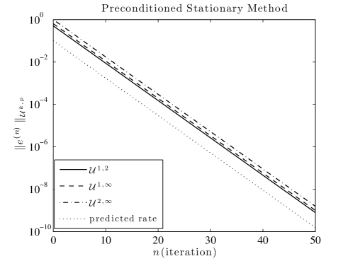
6.4. Numerical example for QCL-preconditioning
We now apply the QCL-preconditioned stationary iterative method to the QCF system with right-hand side (25), , and the optimal value (we note that depends only on and but depends on and independently). The error for successive iterations in the , and -norms are displayed in Figure 2. Even though our theory, in this case, predicts a perfect contractive behavior only in and (partially) in , we nevertheless observe perfect agreement with the optimal predicted rate also in the -norms. As a matter of fact, the parameters are chosen so that case (i) of Theorem 6.2 holds, that is, is not a contraction of . A possible explanation why we still observe this perfect asymptotic behavior is that the norm of is attained in a subspace that is never entered in this iterative process. This is also supported by the fact that the exact solution is uniformly bounded in as , which is a simple consequence of Proposition 3.
7. Preconditioning with QCE (): Ghost-Force Correction
We have shown in [5, 12] that the popular ghost force correction method (GFC) is equivalent to preconditioning the QCF equilibrium equations by the QCE equilibrium equations. The ghost force correction method in a quasi-static loading can thus be reduced to the question whether the iteration matrix
is a contraction. Due to the typical usage of the preconditioner in this case, we do not consider a step size in this section. The purpose of the present section is (i) to investigate whether there exist function spaces in which is a contraction; and (ii) to identify the range of the macroscopic strains where is a contraction.
We begin by recalling the fundamental stability result for the operator, Theorem 2.5:
where with . This result shows that the GFC iteration must necessarily run into instabilities before the deformation reaches the critical strain . This is made precise in the following corollary which states that there is no norm with respect to which is a contraction up to the critical strain .
Corollary 19. Fix and , and let be an arbitrary norm on the space , then, upon understanding as dependent on and , we have
Despite this negative result, we may still be interested in the question of whether the GFC iteration is a contraction in “very stable regimes,” that is, for macroscopic strains which are far away from the critical strain . Naturally, we are particularly interested in the behavior as , that is, we will investigate in which function spaces the operator norm of remains bounded away from one as . Theorem 3 on the unboundedness of immediately provides us with the following negative answer.
Proposition 20. If , , and , then
Proof.
It is an easy exercise to show that, if , then the -norm is equivalent to the norm induced by , that is,
Hence, we have and by the same argument as in the proof of Proposition 6, and using again the uniform norm-equivalence, we can deduce that
∎
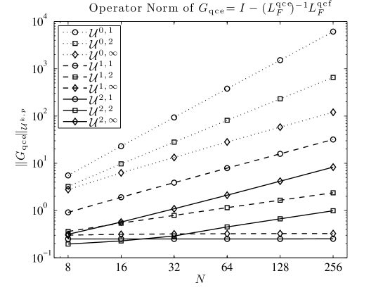
Since the operator is more complicated than that of , which we analyzed in the previous section, we continue to investigate the contraction properties of in various different norms in numerical experiments. In Figure 3, we plot the operator norm of , in the function spaces
against the system size (see Appendix 8.3 for a description of how we compute ). This experiment is performed for which is at some distance from the singularity of (we note that depends only on and since both and depend only on and ). The experiments suggests clearly that as for all norms except for and .
Hence, in a second experiment, we investigate how and behave, for fixed and , as approaches zero. The results of this experiment, which are are displayed in Figure 4, confirm the prediction of Corollary 7 that as approaches zero. Indeed, they show that already much earlier, namely around a strain where and .

Our conclusion based on these analytical results and numerical experiments is that the GFC method is not universally reliable near the limit strain that is, under conditions near the formation or movement of a defect it can fail to converge to a stable solution of the QCF equilibrium equations as the quasi-static loading step tends to zero or the number of GFC iterations tends to infinity. Even though the simple model problem that we investigated here cannot, of course, provide a definite statement, it shows at the very least that further investigations for more realistic model problems are required.
Conclusion
We proposed and studied linear stationary iterative solution methods for the QCF method with the goal of identifying iterative schemes that are efficient and reliable for all applied loads. We showed that, if the local QC operator is taken as the preconditioner, then the iteration is guaranteed to converge to the solution of the QCF system, up to the critical strain. What is interesting is that the choice of function space plays a crucial role in the efficiency of the iterative method. In , the convergence is always uniform in and , however, in this is only true if the macroscopic strain is at some distance from the critical strain. This indicates that, in the presence of defects (that is, non-smooth solutions), the efficiency of a QCL-preconditioned method may be reduced. Further investigations for more realistic model problems are required to shed light on this issue.
We also showed that the popular GFC iteration must necessarily run into instabilities before the deformation reaches the critical strain . Even for macroscopic strains that are far lower than the critical strain we show that We then give numerical experiments that suggest that as for all tested norms except for and
The results presented in this paper demonstrate the challenge for the development of reliable and efficient iterative methods for force-based approximation methods. Further analysis and numerical experiments for two and three dimensional problems are needed to more fully assess the implications of the results in this paper for realistic materials applications.
8. Appendix
8.1. Proof of Theorem 2.5
The purpose of this appendix is to prove the sharp stability result for the operator , formulated in Theorem 2.5. Using Formula (23) in [9] we obtain the following representation of ,
| (29) |
If then we can see from this decomposition that there is a loss of stability at the interaction between atoms and as well as between atoms and . It is therefore natural to test this expression with a displacement defined by
From (29), we easily obtain
In particular, we see that, if then is indefinite. On the other hand, it was shown in [8] that is positive definite provided . (As a matter of fact, the analysis in [8] is for periodic boundary conditions, however, since the Dirichlet displacement space is contained in the periodic displacement space the result is also valid for the present case.)
Thus, we have shown that
To conclude the proof of Theorem 2.5, we need to show that depends only on and that the stated asymptotic result holds.
From (29) it follows that can be written in the form
where we identify with the vector and where . Writing we can see that and that has the entries
Here, the row with entries denotes the th row (in the coordinates ). This form can be verified, for example, by appealing to (29). Let denote the spectrum of a matrix . Since, by assumption, , the smallest eigenvalue of is given by
that is, we need to compute the largest eigenvalue of . Since for and for , and since eigenvectors are orthogonal, we conclude that all other eigenvectors depend only on the submatrix describing the atomistic region and the interface. In particular, depends only on but not on . This proves the claim of Theorem 2.5 that depends indeed only on .
We thus consider the -submatrix , which has the form
Letting , then for ,
and hence, has the general form
leaving undefined for for now, and where are the two roots of the polynomial
In particular, we have
| (30) |
To determine the remaining degrees of freedom, we could now insert this general form into the eigenvalue equation and attempt to solve the resulting problem. This leads to a complicated system which we will try to simplify.
We first note that, for any eigenvector , the vector is also an eigenvector, and hence we can assume without loss of generality that is skew-symmetric about . This implies that . Since the scaling is irrelevant for the eigenvalue problem, we therefore make the ansatz . Next, we notice that for sufficiently large the term is exponentially small and therefore does not contribute to the eigenvalue equation near the right interface. We may safely ignore it if we are only interested in the asymptotics of the eigenvalue as . Thus, letting , and unknown, , we obtain the system
The free parameters can be easily determined from the first two equations. From the final equation we can then compute . Upon recalling from (30) that can be expressed in terms of , and conversely that , we obtain a polynomial equation of degree five for ,
Mathematica was unable to factorize symbolically, hence we computed its roots numerically to twenty digits precision. It turns out that has three real roots and two complex roots. The largest real root is at which gives the value
The relative errors that we had previously neglected are in fact of order , and hence we obtain
This concludes the proof of Theorem 2.5.
8.2. Proofs of Lemmas 6.1 and 6.2
In this appendix, we prove two technical lemmas from Section 6.1. Throughout, the iteration matrix is given by
where and . We begin with the proof of Lemma 6.1, which is more straightforward.
Proof of Lemma 6.1.
Using the basic definition of the operator norm, and the fact that , we obtain
We write the operator as follows:
| (31) |
In the continuum region, we simply obtain
If , we manipulate (31), using the definition of , which yields
In summary, we have obtained
It is now easy to see that
As a matter of fact, in view of the estimate
the upper bound can be reduced to
| (32) |
To show that the bound is attained, we construct a suitable test function. We define via
(note that for any ) and the remaining values of in such a way that . If then there exists at least one function with these properties and it attains the bound (32). Thus, the bound in (32) is an equality, which concludes the proof of the lemma. ∎
Before we prove Lemma 6.2, we recall an explicit representation of that was useful in our analysis in [10]. The proof of the following result is completely analogous to that of [10, Lemma 14] and is therefore sketched only briefly. It is also convenient for the remainder of the section to define the following atomistic and continuum regions for the strains:
Lemma 21. Let and , then
where and are defined as follows:
Proof.
In the notation introduced above, the variational representation of from [10, Sec. 3] reads
Using the fact that and , it is easy to see that the discrete delta-functions appearing in this representation can be rewritten as
Hence, we deduce that the function is given by
In particular, it follows that
where is chosen so that . Since are constructed so that , we only subtract the mean of . Hence, , for which the stated formula is quickly verified. ∎
Proof of Lemma 6.2.
To estimate the first term, we distinguish whether or . A quick computation shows that for . On the other hand, for we have
Since we can thus obtain
| (33) |
As a matter of fact, these bounds can be attained for certain , by choosing suitable test functions. For example, by choosing with we obtain , that is, attains the bound (33). By choosing such that
we obtain that attains the bound (33). In both cases one needs to choose the remaining free so that and , which guarantees that such functions really exist. This can be done under the conditions imposed on and .
To estimate we note that this term depends only on a small number of strains around the interface. We can therefore expand it in terms of these strains and their coefficients and then maximize over all possible interface contributions. Thus, we rewrite as follows:
This expression is maximized by taking to be the sign of the respective coefficient (taking into account also the outer coefficient ), which yields
The equality of the first and second line holds because the terms do not change the signs of the terms inside the bars. Inserting the values for we obtain the bound
and we note that this bound is attained if the values for , , are chosen as described above.
Combining the analyses of the terms and , it follows that
To see that this bound is attained, we note that, under the condition that and , the constructions at the interface to maximize and the constructions to maximize do not interfere. Moreover, under the additional condition , sufficiently many free strains remain to ensure that for a test function , , for which both and attain the stated bound. That is, we have shown that
To conclude the proof, we need to evaluate this maximum explicitly. To this end we first define . For , we have
that is, . Conversely, for , we have
that is, . Since, in , is strictly decreasing and is strictly increasing, there exists a unique such that and such that the stated formula for holds. A straightforward computation yields the value for stated in the lemma. ∎
8.3. Computation of
We have computed for , from the standard formulas for the operator norm [17, 29] of the matrix and with respect to . For and , the norm is also easy to obtain by solving a generalized eigenvalue problem.
The cases and are more difficult. In these cases, the operator norm of in can be estimated in terms of the -operator norm of the conjugate operator (see Lemma 3.2 for an analogous definition of the conjugate operator ). It is not difficult to see that for where we recall that (see Lemma 3.2 similarly for an analogous definition of the restricted conjugate operator ), it follows from (2) that we have only computed for up to a factor of More precisely,
References
- [1] P. Bauman, H. B. Dhia, N. Elkhodja, J. Oden, , and S. Prudhomme. On the application of the Arlequin method to the coupling of particle and continuum models. Computational Mechanics, 42:511–530, 2008.
- [2] T. Belytschko and S. P. Xiao. A bridging domain method for coupling continua with molecular dynamics. Computer Methods in Applied Mechanics and Engineering, 193:1645–1669, 2004.
- [3] N. Bernstein, J. R. Kermode, and G. Cs nyi. Hybrid atomistic simulation methods for materials systems. Reports on Progress in Physics, 72:pp. 026501, 2009.
- [4] X. Blanc, C. Le Bris, and F. Legoll. Analysis of a prototypical multiscale method coupling atomistic and continuum mechanics. M2AN Math. Model. Numer. Anal., 39(4):797–826, 2005.
- [5] M. Dobson and M. Luskin. Analysis of a force-based quasicontinuum approximation. M2AN Math. Model. Numer. Anal., 42(1):113–139, 2008.
- [6] M. Dobson and M. Luskin. Iterative solution of the quasicontinuum equilibrium equations with continuation. Journal of Scientific Computing, 37:19–41, 2008.
- [7] M. Dobson and M. Luskin. An analysis of the effect of ghost force oscillation on the quasicontinuum error. Mathematical Modelling and Numerical Analysis, 43:591–604, 2009.
- [8] M. Dobson and M. Luskin. An optimal order error analysis of the one-dimensional quasicontinuum approximation. SIAM. J. Numer. Anal., 47:2455–2475, 2009.
- [9] M. Dobson, M. Luskin, and C. Ortner. Accuracy of quasicontinuum approximations near instabilities. Journal of the Mechanics and Physics of Solids, 58:1741–1757, 2010. arXiv:0905.2914v2.
- [10] M. Dobson, M. Luskin, and C. Ortner. Sharp stability estimates for force-based quasicontinuum methods. SIAM J. Multiscale Modeling & Simulation, 8:782–802, 2010. arXiv:0907.3861.
- [11] M. Dobson, M. Luskin, and C. Ortner. Stability, instability, and error of the force-based quasicontinuum approximation. Archive for Rational Mechanics and Analysis, 197:179–202, 2010. arXiv:0903.0610.
- [12] M. Dobson, M. Luskin, and C. Ortner. Iterative methods for the force-based quasicontinuum approximation. Computer Methods in Applied Mechanics and Engineering, to appear. arXiv:0910.2013v3.
- [13] M. Dobson, C. Ortner, and A. Shapeev. The spectrum of the force-based quasicontinuum operator for a homogeneous periodic chain. arXiv:1004.3435.
- [14] W. E, J. Lu, and J. Yang. Uniform accuracy of the quasicontinuum method. Phys. Rev. B, 74(21):214115, 2004.
- [15] V. Gavini, K. Bhattacharya, and M. Ortiz. Quasi-continuum orbital-free density-functional theory: A route to multi-million atom non-periodic DFT calculation. J. Mech. Phys. Solids, 55:697–718, 2007.
- [16] M. Gunzburger and Y. Zhang. A quadrature-rule type approximation for the quasicontinuum method. Multiscale Modeling and Simulation, 8:571–590, 2010.
- [17] E. Isaacson and H. Keller. Analysis of Numerical Methods. Wiler, New York, 1966.
- [18] B. V. Koten, X. H. Li, M. Luskin, and C. Ortner. A computational and theoretical investigation of the accuracy of quasicontinuum methods. In I. Graham, T. Hou, O. Lakkis, , and R. Scheichl, editors, Numerical Analysis of Multiscale Problems. Springer, to appear. arXiv:1012.6031.
- [19] B. V. Koten and M. Luskin. Development and analysis of blended quasicontinuum approximations. arXiv:1008.2138v2, 2010.
- [20] X. H. Li and M. Luskin. An analysis of the quasi-nonlocal quasicontinuum approximation of the embedded atom model. IMA Journal of Numerical Analysis, to appear. arXiv:1008.3628v4.
- [21] X. H. Li and M. Luskin. A generalized quasi-nonlocal atomistic-to-continuum coupling method with finite range interaction. International Journal for Multiscale Computational Engineering, to appear. arXiv:1007.2336.
- [22] P. Lin. Convergence analysis of a quasi-continuum approximation for a two-dimensional material without defects. SIAM J. Numer. Anal., 45(1):313–332 (electronic), 2007.
- [23] R. Miller and E. Tadmor. The Quasicontinuum Method: Overview, Applications and Current Directions. Journal of Computer-Aided Materials Design, 9:203–239, 2003.
- [24] R. Miller and E. Tadmor. Benchmarking multiscale methods. Modelling and Simulation in Materials Science and Engineering, 17:053001 (51pp), 2009.
- [25] P. Ming and J. Z. Yang. Analysis of a one-dimensional nonlocal quasicontinuum method. Multiscale Modeling and Simulation, 7:1838–1875, 2009.
- [26] M. Ortiz, R. Phillips, and E. B. Tadmor. Quasicontinuum Analysis of Defects in Solids. Philosophical Magazine A, 73(6):1529–1563, 1996.
- [27] C. Ortner. The role of the patch test in 2d atomistic-to-continuum coupling methods. arXiv:1101.5256, 2011.
- [28] C. Ortner and E. Süli. Analysis of a quasicontinuum method in one dimension. M2AN Math. Model. Numer. Anal., 42(1):57–91, 2008.
- [29] Y. Saad. Iterative Methods for Sparse Linear Systems, volume 2. Society for Industrial and Applied Mathematics (SIAM), 2003.
- [30] A. V. Shapeev. Consistent energy-based atomistic/continuum coupling for two-body potential: 1D and 2D case. arXiv:1010.0512, 2010.
- [31] V. B. Shenoy, R. Miller, E. B. Tadmor, D. Rodney, R. Phillips, and M. Ortiz. An adaptive finite element approach to atomic-scale mechanics–the quasicontinuum method. J. Mech. Phys. Solids, 47(3):611–642, 1999.
- [32] L. E. Shilkrot, R. E. Miller, and W. A. Curtin. Coupled atomistic and discrete dislocation plasticity. Phys. Rev. Lett., 89(2):025501, 2002.
- [33] T. Shimokawa, J. Mortensen, J. Schiotz, and K. Jacobsen. Matching conditions in the quasicontinuum method: Removal of the error introduced at the interface between the coarse-grained and fully atomistic region. Phys. Rev. B, 69(21):214104, 2004.