Default clustering in large portfolios: Typical events

Abstract

We develop a dynamic point process model of correlated default timing in a portfolio of firms, and analyze typical default profiles in the limit as the size of the pool grows. In our model, a firm defaults at a stochastic intensity that is influenced by an idiosyncratic risk process, a systematic risk process common to all firms, and past defaults. We prove a law of large numbers for the default rate in the pool, which describes the “typical” behavior of defaults.

,
and

1 Introduction

The financial crisis of 2007–09 has made clear the need to better understand the diversification of risk in financial systems with interacting entities. Prior to the crisis, the common belief was that risk had been diversified away by using the tools of structured finance. As it turned out, the correlation between assets was much larger than supposed. The collapse fed on itself and created a spiral.

We study the behavior of defaults in a large portfolio of interacting firms. We develop a dynamic point process model of correlated default timing, and then analyze typical default profiles in the limit as the number of constituent firms grows. Our empirically motivated model incorporates two distinct sources of default clustering. First, the firms are exposed to a risk factor process that is common to all entities in the pool. Variations in this systematic risk factor generate correlated movements in firms’ conditional default probabilities. Das, Duffie, Kapadia and Saita ddk show that this mechanism is responsible for a large amount of corporate default clustering in the U.S. Second, a default has a contagious impact on the health of other firms. This impact fades away with time. Azizpour, Giesecke and Schwenkler azizpour-giesecke-schwenkler provide statistical evidence for the presence of such self-exciting effects in U.S. corporate defaults, after controlling for the exposure of firms to systematic risk factors.

More precisely, we assume that a firm defaults at an intensity, or conditional arrival rate, which follows a mean-reverting jump-diffusion process that is driven by several terms. The first term, a square root diffusion, represents an independent, firm-specific source of risk. The second term is a systematic risk factor that influences all firms, and that generates diffusive correlation between the intensities. For simplicity, we take this systematic risk factor to be an Ornstein–Uhlenbeck process. The third term affecting the intensity is the default rate in the pool. Defaults cause jumps in the intensity; they are common to all surviving firms. We thus have two sources of correlation between the firms: the dependence on the systematic risk factor and the influence of past defaults. While this formulation parsimoniously captures several of the sources of default correlation identified in empirical research, the intricate event dependence structure presents a challenge for the mathematical analysis of the system.

Our goal is to understand the behavior of the default rate in the portfolio in the limit as the number of firms in the pool grows. Large stochastic systems often tend to have macroscopic organization due to limit theorems such as the law of large numbers. This allows us to identify typical behavior. Our main result is a law of large numbers for the default rate in the pool; this describes the macroscopically typical profile. The limiting default rate satisfies an integral equation that makes explicit the role of the contagion exposure for the behavior of default clustering in the pool. The result depends heavily on the analysis of Markov processes via the martingale problem; see Ethier and Kurtz MR88a60130 . We will have more to say on the mathematical aspects of this in a moment. Once the typical behavior has been identified, one can then study Gaussian fluctuations and the structure of atypically large default clusters in the portfolio. We plan to pursue these directions in a future work.

Previous studies have analyzed the behavior of defaults in large portfolios. Dembo, Deuschel and Duffie MR2022976 examine a doubly-stochastic model of default timing. In their model, default correlation is due to the exposure of firms to a common systematic risk factor which is represented by a random variable. Conditional on this variable, defaults are independent. A large deviation argument leads to an approximation of the tail of the conditional portfolio loss distribution. Glasserman, Kang and Shahabuddin Glasserman study a copula model of default timing using large deviation techniques. In that formulation, default events are conditionally independent given a set of common risk factors. Bush, Hambly, Haworth, Jin and Reisinger hambly prove a law of large numbers for a related dynamic model. Davis and Rodriguez davis-rod develop a law of large numbers and a central limit theorem for the default rate in a stochastic network setting, in which firms default independently of one another conditional on the realization of a systematic factor governed by a finite state Markov chain. Sircar and Zariphopoulou sircar-zari examine large portfolio asymptotics for utility indifference valuation of securities exposed to the losses in the pool. As with these papers, our model includes exposure to a common systematic risk factor. In contrast, however, our model captures the self-exciting nature of defaults. Therefore, the firms in the pool are correlated even after conditioning on the path of the systematic factor process.

The use of interacting particle systems to study the behavior of default clustering in large portfolios is a growing area. In a mean-field model, Dai Pra, Runggaldier, Sartori and Tolotti daipra-etal and Dai Pra and Tolotti daipra-tolotti take the intensity of a constituent firm as a deterministic function of the percentage portfolio loss due to defaults. In a model with local interaction, Giesecke and Weber giesecke-weber take the intensity of a constituent firm as a deterministic function of the state of the firms in a specified neighborhood of that firm. The interacting particle perspective leads to the study of the convergence of interacting Markov processes, laws of large numbers for the percentage portfolio loss, and Gaussian approximations to the portfolio loss distribution based on central limit theorems. The interacting particle system which we propose and study incorporates an additional source of clustering, namely, the exposure of a firm to a systematic risk factor process. Moreover, firm-specific sources of default risk are present in our system. Also, the nature of mean-field interaction in our system is different. In daipra-etal and daipra-tolotti , a constituent intensity is a function of the current default rate in the pool. In that formulation, the impact of a default on the dynamics of the surviving firms is permanent. In our work, a constituent intensity depends on the path of the default rate. The impact of a default on the surviving firms is transient, and fades away exponentially with time. There is a recovery effect.

As we were finishing this work, we learned of a related law of large numbers type result by Cvitanić, Ma and Zhang CMZ . They take the intensity of a constituent firm as a function of a firm-specific risk factor, a systematic risk factor and the percentage portfolio loss due to defaults. The risk factors follow diffusion processes whose coefficients may depend on the portfolio loss. Our model of the risk factors is more specific than theirs, and thus we are able to arrive at slightly more explicit results. Moreover, the effect of defaults in CMZ is permanent, as in daipra-etal and daipra-tolotti .

There are several mathematical contributions in our efforts. Our analysis of typical events (a weak convergence result) is somewhat similar to that of certain genetic models (most notably the Fleming–Viot process; see Chapter 10 of MR88a60130 , Fleming and Viot FlemingViot and Dawson and Hochberg DawsonHochberg ), but the specific form of our intensity processes imply both complications and simplifications. Our work is centered on a jump-diffusion intensity process which is driven by Ornstein–Uhlenbeck and square root diffusion terms. This formulation allows some explicit simplifying calculations which are not available in a more abstract framework. On the other hand, due to the square root singularity, certain technical estimates need to be developed from scratch (see Section 10). A final point of interest is heterogeneity. Interacting particle systems are often assumed to have homogeneous dynamics, where various parameters are the same for each particle. This allows the main mathematical arguments to take their simplest form. Practitioners in credit risk, however, in reality face an extra problem in data aggregation, where each firm in a portfolio has its own statistical parameters. We have framed our weak convergence result to allow for a distribution of “types,” that is, a frequency count of the different model parameters. This leads us to the correct effective dynamics of the portfolio and, in particular, to a precise formulation of the effects of self-excitation (see Remark 5.2).

The rest of this paper is organized as follows. Section 2 formulates our model of default timing. We establish that our model is well-posed via the results of Section 3. In Section 4 we identify the limit as the number of firms in the portfolio goes to infinity—a law of large numbers result. The proof of this result is in Section 8, but depends upon the technical calculations of Sections 5, 6 and 7. Section 9 concludes and discusses extensions. Section 10 contains a number of technical results on square-root-like processes which are used in our calculations.

2 Model, assumptions and notation

We construct a point process model of correlated default timing in a portfolio of firms. We assume that $(\Omega,\mathscr{F},\mathbb{P})$ is an underlying probability triple on which all random variables are defined. Let $\{W^{n}\}_{n\in\mathbb{N}}$ be a countable collection of standard Brownian motions. Let $\{\mathfrak{e}_{n}\}_{n\in\mathbb{N}}$ be an i.i.d. collection of standard exponential random variables. Finally, let $V$ be a standard Brownian motion which is independent of the $W^{n}$’s and $\mathfrak{e}_{n}$’s. Each $W^{n}$ will represent a source of risk which is idiosyncratic to a specific firm. Each $\mathfrak{e}_{n}$ will represent a normalized default time for a specific firm. The process $V$ will drive a systematic risk factor process to which all firms are exposed.

Fix an $N\in\mathbb{N}$, $n\in\{1,2,\ldots,N\}$ and consider the following system:

$$d\lambda^{N,n}_{t} = -\alpha_{N,n}(\lambda^{N,n}_{t}-\bar{\lambda}_{N,n})\,dt+\sigma_{N,n}\sqrt{\lambda^{N,n}_{t}}\,dW^{n}_{t}$$

$${}+\beta^{C}_{N,n}\,dL^{N}_{t}+\varepsilon_{N}\beta^{S}_{N,n}\lambda^{N,n}_{t}\,dX_{t},\qquad t>0,$$

$$\lambda^{N,n}_{0} = \lambda_{\circ,N,n},$$

$$dX_{t} = -\gamma X_{t}\,dt+dV_{t},\qquad t>0,$$

$$X_{0} = x_{\circ},$$

$$L^{N}_{t} = \frac{1}{N}\sum_{n=1}^{N}\chi_{[\mathfrak{e}_{n},\infty)}\biggl{(}\int_{s=0}^{t}\lambda^{N,n}_{s}\,ds\biggr{)}.$$

Here, $\beta^{C}_{N,n}\in\mathbb{R}_{+}\stackrel{{\scriptstyle\mathrm{def}}}{{=}}[0,\infty)$ and $\beta^{S}_{N,n}\in\mathbb{R}$ are constants which represent the exposure of the $n$th firm in the pool to $L^{N}$ and $X$, respectively. The $\alpha_{N,n}$’s, $\bar{\lambda}_{N,n}$’s and $\sigma_{N,n}$’s are in $\mathbb{R}_{+}$ and characterize the dynamics of the firms. We will address the role of $\varepsilon_{N}$ in a moment. The initial condition $x_{\circ}$ of $X$ is fixed and $\gamma>0$. We use $\chi$ to represent the indicator function here and throughout the paper. The description of $L^{N}$ is equivalent to a more standard construction. In particular, define

$$\tau^{N,n}\stackrel{{\scriptstyle\mathrm{def}}}{{=}}\inf\biggl{\{}t\geq 0\dvtx\int_{s=0}^{t}\lambda^{N,n}_{s}\,ds\geq\mathfrak{e}_{n}\biggr{\}}.$$ (2)

Then

$$\chi_{[\mathfrak{e}_{n},\infty)}\biggl{(}\int_{s=0}^{t}\lambda^{N,n}_{s}\,ds\biggr{)}=\chi_{\{\tau^{N,n}\leq t\}}$$ (3)

and, consequently,

$$L^{N}_{t}=\frac{1}{N}\sum_{n=1}^{N}\chi_{\{\tau^{N,n}\leq t\}}.$$

The process $\lambda^{N,n}$ represents the intensity, or conditional event rate, of the $n$th firm in a portfolio of $N$ firms. More precisely, $\lambda^{N,n}$ is the instantaneous Doob–Meyer compensator to the default indicator process (3); see (6). We will see in Proposition 3.3 in Section 3 that the $\lambda^{N,n}$’s are indeed nonnegative. The process $X$ represents a source of systematic risk; in our model this is a stable Ornstein–Uhlenbeck process. The process $L^{N}$ is the default rate in the pool. The jump-diffusion model for $\lambda^{N,n}$ captures several sources of default clustering. A firm’s intensity is driven by an idiosyncratic source of risk represented by a Brownian motion $W^{n}$, and a source of systematic risk common to all firms—the process $X$. Movements in $X$ cause correlated changes in firms’ intensities and thus provide a source of default clustering emphasized by ddk for corporate defaults in the U.S. The sensitivity of $\lambda^{N,n}$ to changes in $X$ is measured by the parameter $\beta^{S}_{N,n}$. The second source of default clustering is through the feedback (“contagion”) term $\beta^{C}_{N,n}\,dL^{N}_{t}$. A default causes an upward jump of size $\frac{1}{N}\beta^{C}_{N,n}$ in the intensity $\lambda^{N,n}$. Due to the mean-reversion of $\lambda^{N,n}$, the impact of a default fades away with time, exponentially with rate $\alpha_{N,n}$. Self-exciting effects of this type have been found to be an important source of the clustering of defaults in the U.S., over and above any clustering caused by the exposure of firms to systematic risk factors azizpour-giesecke-schwenkler .

In the special case that $\beta^{C}_{N,n}=\beta^{S}_{N,n}=0$ for all $n\in\{1,2,\ldots,N\}$, the intensities $\lambda^{N,n}$ follow independent square root processes so firms default independently of one another. The formulation (2) is a natural generalization of the widely used square root model to address the clustering between defaults.

The interest in large pools of assets is that they provide diversification; they allow one to construct portfolios which have small variance. The dynamics of $X$ imply that $X$ is stochastically of order $1$, that is, it is stable. Thus, the only way for the pool to have small variance in our model is for each of the constituent firms to have small exposure to $X$. We thus assume that

$$\lim_{N\to\infty}\varepsilon_{N}=0.$$

If $\varepsilon_{N}$ is not small, the influence of the systematic risk factor $X$ will be of order 1, and the “typical” behavior of the pool will strongly depend on $X$ (and the tail behavior of the whole system will be strongly determined by the tail of $X$).

Remark 2.1.

Given the simple structure of $X$, our model is equivalent, if $x_{\circ}=0$, to a model where each intensity has exposure of order $1$ to a small systematic risk. Namely, if $x_{\circ}=0$, then $\varepsilon_{N}X=\tilde{X}^{N}$ where

$$d\tilde{X}^{N}_{t}=-\gamma\tilde{X}^{N}_{t}\,dt+\varepsilon_{N}\,dV_{t}.$$

Our model allows for a significant amount of bottom-up heterogeneity; the intensity dynamics of each firm can be different. We capture these different dynamics by defining the “types”

$$\mathsf{p}^{N,n}\stackrel{{\scriptstyle\mathrm{def}}}{{=}}(\alpha_{N,n},\bar{\lambda}_{N,n},\sigma_{N,n},\beta^{C}_{N,n},\beta^{S}_{N,n});$$ (4)

the $\mathsf{p}^{N,n}$’s take values in parameter space $\mathcal{P}\stackrel{{\scriptstyle\mathrm{def}}}{{=}}\mathbb{R}_{+}^{4}\times\mathbb{R}$. In order to expect regular macroscopic behavior of $L^{N}$ as $N\to\infty$, the $\mathsf{p}^{N,n}$’s and the $\lambda_{\circ,N,n}$’s should have enough regularity as $N\to\infty$. For each $N\in\mathbb{N}$, define

$$\pi^{N}\stackrel{{\scriptstyle\mathrm{def}}}{{=}}\frac{1}{N}\sum_{n=1}^{N}\delta_{\mathsf{p}^{N,n}}\quad\mbox{and}\quad\Lambda^{N}_{\circ}\stackrel{{\scriptstyle\mathrm{def}}}{{=}}\frac{1}{N}\sum_{n=1}^{N}\delta_{\lambda_{\circ,N,n}};$$

these are elements of $\mathscr{P}(\mathcal{P})$ and $\mathscr{P}(\mathbb{R}_{+})$, respectively.

We need two main assumptions. First, we assume that the types of (4) and the initial distributions (the $\lambda_{\circ,N,n}$’s) are sufficiently regular.

Assumption 2.2.

We assume that

$$\pi\stackrel{{\scriptstyle\mathrm{def}}}{{=}}\lim_{N\to\infty}\pi^{N}\quad\mbox{and}\quad\Lambda_{\circ}\stackrel{{\scriptstyle\mathrm{def}}}{{=}}\lim_{N\to\infty}\Lambda^{N}_{\circ}$$

exist [in $\mathscr{P}(\mathcal{P})$ and $\mathscr{P}(\mathbb{R}_{+})$, resp.].

Note that this is what happens in practice; one constructs a frequency count of the parameters of the different assets in a large pool and uses this to seek aggregate dynamics for the pool itself. For a large pool, one hopes that this frequency count will have some simpler macroscopic description. Second, we assume that the types are bounded.

Assumption 2.3.

We assume that there is a $K_{\mbox{{\ref{ABounded}}}}>0$ such that the $\alpha_{N,n}$’s, $\bar{\lambda}_{N,n}$’s, $\sigma_{N,n}$’s, $|\beta^{C}_{N,n}|$’s, $|\beta^{S}_{N,n}|$’s and $\lambda_{\circ,N,n}$’s are all bounded by $K_{\mbox{{\ref{ABounded}}}}$ for all $N\in\mathbb{N}$ and $n\in\{1,2,\ldots,N\}$.

Equivalently, we require that the $\pi_{N}$’s and $\Lambda^{N}_{\circ}$’s all (uniformly in $N$) have compact support. We could relax this requirement, at the cost of a much more careful error analysis.

We are interested in the typical behavior of $\{L^{N}\}$. In Section 3 we consider the well-posedness of the model (2), while in Section 4 we state the law of large numbers result, Theorem 4.2.

3 Well-posedness of the model

We here state several technical results concerning the intensities which are a central part of our model. We want to understand the structure of the $\lambda^{N,n}$’s a bit more. The complications which require our attention are the square root singularity, and the fact that the $\lambda_{t}\,dX_{t}$ term contains the term $\lambda_{t}X_{t}\,dt$, implying that the dynamics of the $\mathbb{R}^{2}$-valued process $(\lambda,X)$ contain a superlinear drift. The proofs of the results here will be given in Section 10.

Let $W^{*}$ be a reference Brownian motion with respect to a filtration $\{\mathscr{G}_{t}\}_{t\geq 0}$. Assume also that $V$ is adapted to $\{\mathscr{G}_{t}\}_{t\geq 0}$. Let $\xi$ be a $\{\mathscr{G}_{t}\}_{t\geq 0}$-adapted, point process which takes values in $[0,1]$ and such that $\xi_{0}=0$. Fix $\mathsf{p}=(\alpha,\bar{\lambda},\sigma,\beta^{C},\beta^{S})\in\mathcal{P}$ and $\lambda_{\circ}$ in $\mathbb{R}_{+}$. Consider the SDE

$$d\lambda_{t} = -\alpha(\lambda_{t}-\bar{\lambda})\,dt+\sigma\sqrt{\lambda_{t}\vee 0}\,dW^{*}_{t}+\beta^{C}\,d\xi_{t}+\beta^{S}\lambda_{t}\,dX_{t},\qquad t>0,$$

$$\lambda_{0} = \lambda_{\circ}.$$

Note that by expanding the dynamics of $dX$ and rearranging a bit, we get that

$$d\lambda_{t}=-\{\alpha+\beta^{S}\gamma X_{t}\}\lambda_{t}\,dt+\alpha\bar{\lambda}\,dt+\beta^{C}\,d\xi_{t}+\sigma\sqrt{\lambda_{t}\vee 0}\,dW^{*}_{t}+\beta^{S}\lambda_{t}\,dV_{t}.$$

Also, we have for the moment subsumed the small parameter $\varepsilon_{N}$ into the $\beta^{S}$ term; see the proof of Proposition 3.3.

We will use a number of ideas from MR1011252 (see also Deelsra-Delbaen ).

Lemma 3.1

There is a nonnegative solution $\lambda$ of the $\mathbb{R}$-valued SDE (3). Furthermore, $\sup_{t\in[0,T]}\mathbb{E}[|\lambda_{t}|^{p}]<\infty$ for all $T>0$ and $p\geq 1$.

We also have uniqueness.

Lemma 3.2

The solution of (3) is unique.

The model (2) is thus well posed.

Proposition 3.3

The system (2) has a unique solution such that $\lambda^{N,n}_{t}\geq 0$ for every $N\in\mathbb{N}$, $n\in\{1,2,\ldots,N\}$ and $t\geq 0$.

Using Lemmas 3.1 and 3.2, solve (2) between the default times. Replace $\beta^{S}$ by $\varepsilon_{N}\beta^{S}$ in applying Lemma 3.1.

We shall also need a macroscopic bound on the intensities.

Lemma 3.4

For each $p\geq 1$ and $T\geq 0$,

$$K_{p,T,\mbox{{\ref{Lmacrobound}}}}\stackrel{{\scriptstyle\mathit{def}}}{{=}}\mathop{\sup_{0\leq t\leq T}}_{N\in\mathbb{N}}\frac{1}{N}\sum_{n=1}^{N}\mathbb{E}[|\lambda^{N,n}_{t}|^{p}]$$

is finite.

4 Typical events: A law of large numbers

Our first task is to understand the “typical” behavior of our system. To do so, we need to understand a system which contains a bit more information than the default rate $L^{N}$. For each $N\in\mathbb{N}$ and $n\in\{1,2,\ldots,N\}$, define

$$\mbox{{m}}^{N,n}_{t}\stackrel{{\scriptstyle\mathrm{def}}}{{=}}\chi_{[0,\mathfrak{e}_{n})}\biggl{(}\int_{s=0}^{t}\lambda^{N,n}_{s}\,ds\biggr{)}=\chi_{\{\tau^{N,n}>t\}}$$ (6)

[where $\tau^{N,n}$ is as in (2)]. In other words, $\mbox{{m}}^{N,n}_{t}=1$ if and only if the $n$th firm is still alive at time $t$; otherwise $\mbox{{m}}^{N,n}_{t}=0$. Thus, $\mbox{{m}}^{N,n}$ is nonincreasing and right-continuous. It is easy to see that

$$\mbox{{m}}^{N,n}_{t}+\int_{s=0}^{t}\lambda^{N,n}_{s}\mbox{{m}}^{N,n}_{s}\,ds$$

is a martingale. Define $\hat{\mathcal{P}}\stackrel{{\scriptstyle\mathrm{def}}}{{=}}\mathcal{P}\times\mathbb{R}_{+}$. For each $N\in\mathbb{N}$, define $\hat{\mathsf{p}}^{N,n}_{t}\stackrel{{\scriptstyle\mathrm{def}}}{{=}}(\mathsf{p}^{N,n},\lambda^{N,n}_{t})$ for all $n\in\{1,2,\ldots,N\}$ and $t\geq 1$. For each $t\geq 0$, define

$$\mu^{N}_{t}\stackrel{{\scriptstyle\mathrm{def}}}{{=}}\frac{1}{N}\sum_{n=1}^{N}\delta_{\hat{\mathsf{p}}^{N,n}_{t}}\mbox{{m}}^{N,n}_{t};$$

in other words, we keep track of the empirical distribution of the type and credit spread for those assets which are still “alive.” We note that

$$L^{N}_{t}=1-\mu^{N}_{t}(\hat{\mathcal{P}})$$

for all $t\geq 0$.

We want to understand the dynamics of $\mu^{N}_{t}$ for large $N$ (this will then imply the “typical” behavior for $L^{N}_{t}$). To understand what our main result is, let’s first set up a topological framework to understand convergence of $\mu^{N}$. Let $E$ be the collection of sub-probability measures (i.e., defective probability measures) on $\hat{\mathcal{P}}$, that is, $E$ consists of those Borel measures $\nu$ on $\hat{\mathcal{P}}$ such that $\nu(\hat{\mathcal{P}})\leq 1$. We can topologize $E$ in the usual way (by projecting onto the one-point compactification of $\hat{\mathcal{P}}$; see MR90g00004 , Chapter 9.5). In particular, fix a point $\star$ that is not in $\hat{\mathcal{P}}$ and define $\hat{\mathcal{P}}^{+}\stackrel{{\scriptstyle\mathrm{def}}}{{=}}\hat{\mathcal{P}}\cup\{\star\}$. Give $\hat{\mathcal{P}}^{+}$ the standard topology; open sets are those which are open subsets of $\hat{\mathcal{P}}$ (with its original topology) or complements in $\hat{\mathcal{P}}^{+}$ of closed subsets of $\hat{\mathcal{P}}$ (again, in the original topology of $\hat{\mathcal{P}}$). Define a bijection $\iota$ from $E$ to $\mathscr{P}(\hat{\mathcal{P}}^{+})$ (the collection of Borel probability measures on $\hat{\mathcal{P}}^{+}$) by setting

$$(\iota\nu)(A)\stackrel{{\scriptstyle\mathrm{def}}}{{=}}\nu(A\cap\hat{\mathcal{P}})+\bigl{(}1-\nu(\hat{\mathcal{P}})\bigr{)}\delta_{\star}(A)$$

for all $A\in\mathscr{B}(\hat{\mathcal{P}}^{+})$. We can define the Skorohod topology on $\mathscr{P}(\hat{\mathcal{P}}^{+})$, and define a corresponding metric on $E$ by requiring $\iota$ to be an isometry. This makes $E$ a Polish space. We thus have that $\mu^{N}$ is an element of $D_{E}[0,\infty)$.

The main theorem of this section is Theorem 4.2, essentially a law of large numbers. The construction of the limiting process will take several steps. First, for each $\mathsf{p}=(\alpha,\bar{\lambda},\sigma,\beta^{C},\beta^{S})\in\mathcal{P}$, let $b^{\mathsf{p}}$ satisfy

$$\dot{b}^{\mathsf{p}}(t) = 1-\tfrac 12\sigma^{2}(b^{\mathsf{p}}(t))^{2}-\alpha b^{\mathsf{p}}(t),\qquad t>0,$$

$$b^{\mathsf{p}}(0) = 0.$$

Note that if $b^{\mathsf{p}}(t)=0$, then $\dot{b}^{\mathsf{p}}(t)=1>0$. Thus, $b^{\mathsf{p}}(t)>0$ for all $t>0$.

The next lemma is essential for the characterization of the limit. Its proof is deferred to Section 10.

Lemma 4.1

There is a unique $\mathbb{R}_{+}$-valued trajectory $\{Q(t);t\geq 0\}$ which satisfies the equation

$$Q(t) = \mathop{\int_{\hat{\mathsf{p}}=(\mathsf{p},\lambda)\in\hat{\mathcal{P}}}}_{\mathsf{p}=(\alpha,\bar{\lambda},\sigma,\beta^{C},\beta^{S})}\beta^{C}\biggl{[}\dot{b}^{\mathsf{p}}(t)\lambda+\int_{r=0}^{t}\dot{b}^{\mathsf{p}}(t-r)\{Q(r)+\alpha\bar{\lambda}\}\,dr\biggr{]}$$

$$\hskip 61.0pt{}\times\exp\biggl{[}-b^{\mathsf{p}}(t)\lambda-\int_{r=0}^{t}b^{\mathsf{p}}(t-r)\{Q(r)+\alpha\bar{\lambda}\}\,dr\biggr{]}$$

$$\hskip 61.0pt{}\times\pi(d\mathsf{p})\Lambda_{\circ}(d\lambda).$$

Here, $\pi$ and $\Lambda_{\circ}$ are as in Assumption 2.2.

Now let $W^{*}$ be a reference Brownian motion. For each $\hat{\mathsf{p}}=(\mathsf{p},\lambda_{\circ})\in\hat{\mathcal{P}}$ where $\mathsf{p}=(\alpha,\bar{\lambda},\sigma,\beta^{C},\beta^{S})$, let $\lambda^{*}_{t}(\mathsf{p})$ be the unique solution to

$$\lambda^{*}_{t}(\hat{\mathsf{p}}) = \lambda_{\circ}-\alpha\int_{s=0}^{t}\bigl{(}\lambda^{*}_{s}(\hat{\mathsf{p}})-\bar{\lambda}\bigr{)}\,ds+\sigma\int_{s=0}^{t}\sqrt{\lambda^{*}_{s}(\hat{\mathsf{p}})}\,dW^{*}_{s}$$

$${}+\int_{s=0}^{t}Q(s)\,ds.$$

We now have our main result.

Theorem 4.2

For all $A\in\mathscr{B}(\mathcal{P})$ and $B\in\mathscr{B}(\mathbb{R}_{+})$, define

$$\bar{\mu}_{t}(A\times B) \stackrel{{\scriptstyle\mathit{def}}}{{=}} \int_{\hat{\mathsf{p}}=(\mathsf{p},\lambda)\in\hat{\mathcal{P}}}\chi_{A}(\mathsf{p})\mathbb{E}\biggl{[}\chi_{B}(\lambda^{*}_{t}(\hat{\mathsf{p}}))\exp\biggl{[}-\int_{s=0}^{t}\lambda_{s}^{*}(\hat{\mathsf{p}})\,ds\biggr{]}\biggr{]}$$

$$\hskip 45.0pt{}\times\pi(d\mathsf{p})\Lambda_{\circ}(d\lambda).$$

Then

$$\lim_{N\to\infty}\mathbb{P}\bigl{\{}d_{\mathscr{P}(\hat{\mathcal{P}})}(\mu^{N},\bar{\mu})\geq\delta\bigr{\}}=0$$ (11)

for every $\delta>0$. Define

$$F(t)\stackrel{{\scriptstyle\mathit{def}}}{{=}}1-\bar{\mu}_{t}(\hat{\mathcal{P}})$$

(12)

$$\qquad=1-\int_{\hat{\mathsf{p}}=(\mathsf{p},\lambda)\in\hat{\mathcal{P}}}\mathbb{E}\biggl{[}\exp\biggl{[}-\int_{s=0}^{t}\lambda_{s}^{*}(\hat{\mathsf{p}})\,ds\biggr{]}\biggr{]}\pi(d\mathsf{p})\Lambda_{\circ}(d\lambda).$$

Then, for all $\delta>0$ and $T>0$,

$$\lim_{N\to\infty}\mathbb{P}\Bigl{\{}\sup_{0\leq t\leq T}|L^{N}_{t}-F(t)|\geq\delta\Bigr{\}}=0.$$

The parts of the proof of this result will be given in Sections 5, 6 and 7. In particular, in Section 5 we identify a candidate limit for $\{\mu^{N}\}$ using the martingale problem formulation. Then in Section 6 we prove that $\{\mu^{N}\}$ is tight, which ensures that the laws of $\{\mu^{N}\}$’s have at least one limit point. In Section 7 we prove that the limit is necessarily unique. Then, in Section 8 we collect things together to prove Theorem 4.2.

With this result in hand, we can rewrite (4) to see the exposure of a typical firm to the contagion factor.

Remark 4.3.

We have that

$$\dot{F}(t) = \int_{\hat{\mathsf{p}}=(\mathsf{p},\lambda)\in\hat{\mathcal{P}}}\mathbb{E}\biggl{[}\lambda_{t}^{*}(\hat{\mathsf{p}})\exp\biggl{[}-\int_{s=0}^{t}\lambda_{s}^{*}(\hat{\mathsf{p}})\,ds\biggr{]}\biggr{]}\pi(d\mathsf{p})\Lambda_{\circ}(d\lambda)$$

$$= \int_{\hat{\mathsf{p}}=(\mathsf{p},\lambda)\in\hat{\mathcal{P}}}\lambda\bar{\mu}_{t}(d\hat{\mathsf{p}}).$$

Thus,

$$\lambda^{*}_{t}(\hat{\mathsf{p}}) = \lambda_{\circ}-\alpha\int_{s=0}^{t}\bigl{(}\lambda^{*}_{s}(\hat{\mathsf{p}})-\bar{\lambda}\bigr{)}\,ds+\sigma\int_{0}^{t}\sqrt{\lambda^{*}_{s}(\hat{\mathsf{p}})}\,dW^{*}_{s}$$

$${}+\int_{0}^{t}B(\bar{\mu}_{s})\dot{F}(s)\,ds,$$

where

$$B(\mu)\stackrel{{\scriptstyle\mathrm{def}}}{{=}}\mathop{\int_{\hat{\mathsf{p}}=(\mathsf{p},\lambda)\in\hat{\mathcal{P}}}}_{\mathsf{p}=(\alpha,\bar{\lambda},\sigma,\beta^{C},\beta^{S})}\beta^{C}\lambda\mu(d\hat{\mathsf{p}})\Big{/}\mathop{\int_{\hat{\mathsf{p}}=(\mathsf{p},\lambda)\in\hat{\mathcal{P}}}}_{\mathsf{p}=(\alpha,\bar{\lambda},\sigma,\beta^{C},\beta^{S})}\lambda\mu(d\hat{\mathsf{p}})$$

for all $\mu\in E$. In other words, the effective sensitivity of a typical intensity to the contagion is given by an average weighted by the instantaneous intensities. Note that $0\leq B(\mu)\leq K_{\mbox{{\ref{ABounded}}}}$.

The homogeneous case provides more explicit insights into the role of the contagion exposure for the behavior of default clustering in the pool.

Remark 4.4.

Fix $\hat{\mathsf{p}}=(\mathsf{p},\lambda_{\circ})\in\hat{\mathcal{P}}$ where $\mathsf{p}=(\alpha,\bar{\lambda},\sigma,\beta^{C},\beta^{S})$. Assume that the pool is homogeneous, that is, $\hat{\mathsf{p}}^{N,n}=\hat{\mathsf{p}}$ for all $N\in\mathbb{N}$ and $n\in\{1,2,\ldots,N\}$. By the relation (4.3), we then have that $Q(t)=\beta^{C}\dot{F}(t)$. In this case, $F$ is given by the unique solution to the integral equation

$$F(t)=1-\exp\biggl{[}-\alpha\bar{\lambda}\int_{r=0}^{t}b^{\mathsf{p}}(t-r)\,dr-\beta^{C}\int_{r=0}^{t}F(r)\dot{b}^{\mathsf{p}}(t-r)\,dr-b^{\mathsf{p}}(t)\lambda_{\circ}\biggr{]}.$$

Furthermore, if there is no exposure to contagion, that is, $\beta^{C}=0$, then this integral equation reduces to the well-known explicit formula

$$F(t)=1-\exp\biggl{[}-\alpha\bar{\lambda}\int_{r=0}^{t}b^{\mathsf{p}}(t-r)\,dr-b^{\mathsf{p}}(t)\lambda_{\circ}\biggr{]}.$$

Figure 1 shows the limiting default rate $F(t)$ for different values of the contagion sensitivity $\beta^{C}$. The default rate increases with $\beta^{C}$. Figure 2 shows the limiting default rate $F(t)$ for different values of the parameter $\alpha$, which

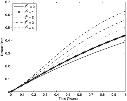
Figure 1: Comparison of limiting default rate $F(t)$ for different values of the contagion sensitivity $\beta^{C}$. The parameter case is $\sigma=0.9$, $\alpha=4$, $\bar{\lambda}=0.5$ and $\lambda_{0}=0.5$.

specifies the reversion speed of the intensity. The default rate is relatively insensitive to changes in $\alpha$ for shorter horizons; for longer horizons it decreases with $\alpha$. The limiting default rate

Figure 2: Comparison of limiting default rate $F(t)$ for different values of the reversion speed $\alpha$. The parameter case is $\sigma=0.9$, $\beta^{C}=2$, $\bar{\lambda}=0.5$ and $\lambda_{0}=0.5$.

is more sensitive to variation in the reversion level $\bar{\lambda}$, as indicated in Figure 3. Variations in the diffusive volatility $\sigma$ of the intensity have little effect on $F(t)$.

Figure 3: Comparison of limiting default rate $F(t)$ for different values of the reversion level $\bar{\lambda}$. The parameter case is $\sigma=0.9$, $\beta^{C}=2$, $\alpha=4$ and $\lambda_{0}=0.5$.

We finally note that the structure of the unperturbed (i.e., $\beta^{C}=\beta^{S}=0$) dynamics of the intensity (2) was crucial in singling out the equation (4.1) as the proper macroscopic effect of the contagion (see the proof of Lemma 8.2). The calculations in fact hinge upon the explicit formulae for affine jump diffusions developed in DuffiePanSingleton . In a more general setting we would need a more abstract framework (see CMZ ).

5 Identification of the limit

We want to use the martingale problem (see Chapter 4 of MR88a60130 ) to show that $\mu^{N}$’s converge to a limiting process. For every $f\in C^{\infty}(\hat{\mathcal{P}})$ and $\mu\in E$, define

$$\langle f,\mu\rangle_{E}\stackrel{{\scriptstyle\mathrm{def}}}{{=}}\int_{\hat{\mathsf{p}}\in\hat{\mathcal{P}}}f(\hat{\mathsf{p}})\mu(d\hat{\mathsf{p}}).$$

Let $\mathcal{S}$ be the collection of elements $\Phi$ in $B(\mathscr{P}(\hat{\mathcal{P}}))$ of the form

$$\Phi(\mu)=\varphi(\langle f_{1},\mu\rangle_{E},\langle f_{2},\mu\rangle_{E},\ldots,\langle f_{M},\mu\rangle_{E})$$ (15)

for some $M\in\mathbb{N}$, some $\varphi\in C^{\infty}(\mathbb{R}^{M})$ and some $\{f_{m}\}_{m=1}^{M}$. Then $\mathcal{S}$ separates $\mathscr{P}(\hat{\mathcal{P}})$ (see Chapter 3.4 of MR88a60130 ). It thus suffices to show convergence of the martingale problem for functions of the form (15).

Let’s fix $f\in C^{\infty}(\hat{\mathcal{P}})$ and understand exactly what happens to $\langle f,\mu^{N}\rangle_{E}$ when one of the firms defaults. Suppose that the $n$th firm defaults at time $t$ and that none of the other firms default at time $t$ (defaults occur simultaneously with probability zero). Then

$$\langle f,\mu^{N}_{t}\rangle_{E} = \frac{1}{N}\mathop{\sum_{1\leq n^{\prime}\leq N}}_{n^{\prime}\not=n}f\biggl{(}\mathsf{p}^{N,n^{\prime}},\lambda^{N,n^{\prime}}_{t}+\frac{\beta^{C}_{N,n}}{N}\biggr{)}\mbox{{m}}^{N,n^{\prime}}_{t},$$

$$\langle f,\mu^{N}_{t-}\rangle_{E} = \frac{1}{N}f(\mathsf{p}^{N,n^{\prime}},\lambda^{N,n^{\prime}}_{t})\mbox{{m}}^{N,n^{\prime}}_{t}+\frac{1}{N}f(\mathsf{p}^{N,n},\lambda^{N,n}_{t}).$$

Note, furthermore, that the default at time $t$ means that $\int_{s=0}^{t}\lambda^{N,n}_{s}\,ds=\mathfrak{e}_{n}$, so $\mbox{{m}}^{N,n}_{t}=0$. Hence,

$$\langle f,\mu^{N}_{t}\rangle_{E}-\langle f,\mu^{N}_{t-}\rangle_{E}=\mathcal{J}^{f}_{N,n}(t),$$ (16)

where

$$\mathcal{J}^{f}_{N,n}(t) \stackrel{{\scriptstyle\mathrm{def}}}{{=}} \frac{1}{N}\sum_{n^{\prime}=1}^{N}\biggl{\{}f\biggl{(}\mathsf{p}^{N,n^{\prime}},\lambda^{N,n^{\prime}}_{t}+\frac{\beta^{C}_{N,n}}{N}\biggr{)}-f(\mathsf{p}^{N,n^{\prime}},\lambda^{N,n^{\prime}}_{t})\biggr{\}}\mbox{{m}}^{N,n^{\prime}}_{t}$$

$${}-\frac{1}{N}f(\mathsf{p}^{N,n},\lambda^{N,n}_{t})$$

for all $t\geq 0$, $N\in\mathbb{N}$ and $n\in\{1,2,\ldots,N\}$.

We now identify the limiting martingale problem for $\mu^{N}$. For $\hat{\mathsf{p}}=(\mathsf{p},\lambda)$ where $\mathsf{p}=(\alpha,\bar{\lambda},\sigma,\beta^{C},\beta^{S})\in\mathcal{P}$ and $f\in C^{\infty}(\hat{\mathcal{P}})$, define the operators

$$(\mathcal{L}_{1}f)(\hat{\mathsf{p}}) = \frac{1}{2}\sigma^{2}\lambda\,\frac{\partial^{2}f}{\partial\lambda^{2}}(\hat{\mathsf{p}})-\alpha(\lambda-\bar{\lambda})\,\frac{\partial f}{\partial\lambda}(\hat{\mathsf{p}})-\lambda f(\hat{\mathsf{p}}),$$

$$(\mathcal{L}_{2}f)(\hat{\mathsf{p}}) = \frac{\partial f}{\partial\lambda}(\hat{\mathsf{p}}).$$

Define also

$$\mathcal{Q}(\hat{\mathsf{p}})\stackrel{{\scriptstyle\mathrm{def}}}{{=}}\lambda\beta^{C}$$

for $\hat{\mathsf{p}}=(\mathsf{p},\lambda)$ where $\mathsf{p}=(\alpha,\bar{\lambda},\sigma,\beta^{C},\beta^{S})\in\mathcal{P}$. The generator $\mathcal{L}_{1}$ corresponds to the diffusive part of the intensity with killing rate $\lambda$, and $\mathcal{L}_{2}$ is the macroscopic effect of contagion on the surviving intensities at any given time. For $\Phi\in\mathcal{S}$ of the form (15), define

$$(\mathcal{A}\Phi)(\mu)\stackrel{{\scriptstyle\mathrm{def}}}{{=}}\sum_{m=1}^{M}\frac{\partial\varphi}{\partial x_{m}}(\langle f_{1},\mu\rangle_{E},\langle f_{2},\mu\rangle_{E},\ldots,\langle f_{M},\mu\rangle_{E})$$

(18)

$$\hskip 74.0pt{}\times\{\langle\mathcal{L}_{1}f_{m},\mu\rangle_{E}+\langle\mathcal{Q},\mu\rangle_{E}\langle\mathcal{L}_{2}f_{m},\mu\rangle_{E}\}.$$

We claim that $\mathcal{A}$ will be the generator of the limiting martingale problem.

Lemma 5.1 ((Weak convergence))

For any $\Phi\in\mathcal{S}$ and $0\leq r_{1}\leq r_{2}\cdots r_{J}=s<t<T$ and $\{\psi_{j}\}_{j=1}^{J}\subset B(E)$, we have that

$$\lim_{N\to\infty}\mathbb{E}\Biggl{[}\biggl{\{}\Phi(\mu^{N}_{t})-\Phi(\mu^{N}_{s})-\int_{r=s}^{t}(\mathcal{A}\Phi)(\mu^{N}_{r})\,dr\biggr{\}}\prod_{j=1}^{J}\psi_{j}(\mu^{N}_{r_{j}})\Biggr{]}=0.$$

For $\hat{\mathsf{p}}=(\mathsf{p},\lambda)$ where $\mathsf{p}=(\alpha,\bar{\lambda},\sigma,\beta^{C},\beta^{S})\in\mathcal{P}$, define

$$(\mathcal{L}^{a}f)(\hat{\mathsf{p}}) = \frac{1}{2}\sigma^{2}\lambda\,\frac{\partial^{2}f}{\partial\lambda^{2}}(\hat{\mathsf{p}})-\alpha(\lambda-\bar{\lambda})\,\frac{\partial f}{\partial\lambda}(\hat{\mathsf{p}}),$$

$$(\mathcal{L}_{x}^{b}f)(\hat{\mathsf{p}}) = \lambda\biggl{\{}\frac{1}{2}\,\frac{\partial^{2}f}{\partial\lambda^{2}}(\hat{\mathsf{p}})-\gamma x\,\frac{\partial f}{\partial\lambda}(\hat{\mathsf{p}})\biggr{\}},\qquad x\in\mathbb{R}.$$

Then $\mathcal{L}^{a}$ is the generator of the idiosyncratic part of the intensity and $\mathcal{L}^{b}_{x}$ is the generator of the systematic risk.

We start by writing that

$$\Phi(\mu^{N}_{t})=\Phi(\mu^{N}_{0})+\int_{r=0}^{t}\{A^{N,1}_{r}+A^{N,2}_{r}\}\,dr+\mathcal{M}_{t},$$

where $\mathcal{M}$ is a martingale and

$$A^{N,1}_{t} = \sum_{m=1}^{M}\frac{\partial\varphi}{\partial x_{m}}(\langle f_{1},\mu^{N}_{t}\rangle_{E},\langle f_{2},\mu^{N}_{t}\rangle_{E},\ldots,\langle f_{M},\mu^{N}_{t}\rangle_{E})$$

$$\hskip 16.1pt{}\times\frac{1}{N}\sum_{n=1}^{N}\{(\mathcal{L}^{a}f_{m})(\hat{\mathsf{p}}^{N,n}_{t})+\varepsilon_{N}(\mathcal{L}^{b}_{X_{t}}f_{m})(\hat{\mathsf{p}}^{N,n}_{t})\}\mbox{{m}}^{N,n}_{t}$$

$$= \sum_{m=1}^{M}\frac{\partial\varphi}{\partial x_{m}}(\langle f_{1},\mu^{N}_{t}\rangle_{E},\langle f_{2},\mu^{N}_{t}\rangle_{E},\ldots,\langle f_{M},\mu^{N}_{t}\rangle_{E})$$

$$\hskip 16.1pt{}\times\{\langle\mathcal{L}^{a}f_{m},\mu^{N}_{t}\rangle_{E}+\varepsilon_{N}\langle\mathcal{L}_{X_{t}}^{b}f_{m},\mu^{N}_{t}\rangle_{E}\},$$

$$A^{N,2}_{t} = \sum_{n=1}^{N}\lambda^{N,n}_{t}\bigl{\{}\varphi\bigl{(}\langle f_{1},\mu^{N}_{t}\rangle_{E}+\mathcal{J}^{f_{1}}_{N,n}(t),$$

$$\hskip 53.5pt\langle f_{2},\mu^{N}_{t}\rangle_{E}+\mathcal{J}^{f_{2}}_{N,n}(t),\ldots,\langle f_{M},\mu^{N}_{t}\rangle_{E}+\mathcal{J}^{f_{M}}_{N,n}(t)\bigr{)}$$

$$\hskip 34.3pt\hskip 39.0pt{}-\varphi(\langle f_{1},\mu^{N}_{t}\rangle_{E},\langle f_{2},\mu^{N}_{t}\rangle_{E},\ldots,\langle f_{M},\mu^{N}_{t}\rangle_{E})\bigr{\}}\mbox{{m}}^{N,n}_{t}.$$

Using Lemma 3.4, it is fairly easy to see that for all $f\in C^{\infty}(\hat{\mathcal{P}})$,

$$\lim_{N\rightarrow\infty}\mathbb{E}\biggl{[}\varepsilon_{N}\int_{r=0}^{t}|\langle\mathcal{L}_{X_{r}}^{b}f,\mu^{N}_{r}\rangle_{E}|\,dr\biggr{]}=0.$$

To proceed, let’s simplify $\mathcal{J}^{f}_{N,n}$. For each $f\in C^{\infty}(\hat{\mathcal{P}})$, $t\geq 0$, $N\in\mathbb{N}$ and $n\in\{1,2,\ldots,N\}$, define

$$\tilde{\mathcal{J}}^{f}_{N,n}(t) \stackrel{{\scriptstyle\mathrm{def}}}{{=}} \frac{\beta^{C}_{N,n}}{N}\sum_{m=1}^{N}\frac{\partial f}{\partial\lambda}(\hat{\mathsf{p}}^{N,n}_{t})\mbox{{m}}^{N,m}_{t}-f(\mathsf{p}^{N,n},\lambda^{N,n}_{t})$$

$$= \beta^{C}_{N,n}\langle\mathcal{L}_{2}f,\mu^{N}_{t}\rangle_{E}-f(\hat{\mathsf{p}}^{N}_{t}).$$

Then

$$\biggl{|}\mathcal{J}^{f}_{N,n}(t)-\frac{1}{N}\tilde{\mathcal{J}}^{f}_{N,n}(t)\biggr{|}\leq\frac{K_{\mbox{{\ref{ABounded}}}}^{2}}{N^{2}}\biggl{\|}\frac{\partial^{2}f}{\partial\lambda^{2}}\biggr{\|}_{C},$$

where $K_{\mbox{{\ref{ABounded}}}}$ is the constant from Assumption 2.3.

Define $\iota(\hat{\mathsf{p}})\stackrel{{\scriptstyle\mathrm{def}}}{{=}}\lambda$ for $\hat{\mathsf{p}}=(\mathsf{p},\lambda)\in\hat{\mathcal{P}}$. Setting

$$\tilde{A}^{N,2}_{t} \stackrel{{\scriptstyle\mathrm{def}}}{{=}} \sum_{m=1}^{M}\frac{\partial\varphi}{\partial x_{m}}(\langle f_{1},\mu^{N}_{t}\rangle_{E},\langle f_{2},\mu^{N}_{t}\rangle_{E},\ldots,\langle f_{M},\mu^{N}_{t}\rangle_{E})$$

$$\hskip 16.3pt{}\times\frac{1}{N}\sum_{n=1}^{N}\lambda^{N,n}_{t}\tilde{\mathcal{J}}^{f_{m}}_{N,n}(t)\mbox{{m}}^{N,n}_{t}$$

$$= \sum_{m=1}^{M}\frac{\partial\varphi}{\partial x_{m}}(\langle f_{1},\mu^{N}_{t}\rangle_{E},\langle f_{2},\mu^{N}_{t}\rangle_{E},\ldots,\langle f_{M},\mu^{N}_{t}\rangle_{E})$$

$$\hskip 16.8pt{}\times\{\langle\mathcal{Q},\mu^{N}_{t}\rangle_{E}\langle\mathcal{L}_{2}f_{m},\mu^{N}_{t}\rangle_{E}-\langle\iota f,\mu^{N}_{t}\rangle_{E}\},$$

we have that

$$\lim_{N\to\infty}\mathbb{E}\biggl{[}\int_{r=0}^{t}|A^{N,2}_{r}-\tilde{A}^{N,2}_{r}|\,dr\biggr{]}=0.$$

Collecting things together, we have that

$$\lim_{N\to\infty}\mathbb{E}\Biggl{[}\biggl{\{}\int_{r=s}^{t}A^{N,1}_{r}\,dr+\int_{r=s}^{t}A^{N,2}_{r}\,dr-\int_{r=s}^{t}(\mathcal{A}\Phi)(\mu^{N}_{r})\,dr\biggr{\}}\prod_{j=1}^{J}\psi_{j}(\mu^{N}_{r_{j}})\Biggr{]}=0,$$

which implies the claim.

We, in particular, note the macroscopic effect of the contagion.

Remark 5.2.

The key step in quantifying the coarse-grained effect of contagion was (5). Namely, we average the combination of the jump rate and the exposure to contagion across the pool.

6 Tightness

In this subsection we verify that the family $\{\mu^{N}\}_{N\in\mathbb{N}}$ is relatively compact (as a $D_{E}[0,\infty)$-valued random variable); this of course is necessary to ensure that the laws of the $\mu^{N}$’s have at least one limit point. The complication of course is the feedback through contagion. We need to show that the system is unlikely to “explode” via feedback. Our calculations are framed by Theorem 8.6 of Chapter 3 of MR88a60130 ; we need to show compact containment and regularity of the $\mu^{N}$’s.

In particular, compact containment ensures that there is a compact set $\mathcal{K}$ such that $\mu^{N}_{t}$ will belong to $\mathcal{K}$ for all $N\in\mathbb{N}$ and $t\in[0,T]$ with high probability; see Lemma 6.1. Regularity shows, roughly speaking, that $\mu^{N}_{t}-\mu^{N}_{s}$ is bounded in a certain sense by a function of the time interval $t-s$, that goes to zero as the length of the time interval goes to zero; see Lemma 6.3. By Theorem 8.6 of Chapter 3 of MR88a60130 , these two statements imply relative compactness of the family $\{\mu^{N}\}_{N\in\mathbb{N}}$ in $D_{E}[0,\infty)$; see Lemma 6.4.

Let’s first address compact containment.

Lemma 6.1

For each $\eta>0$ and $t\geq 0$, there is a compact subset $\mathcal{K}$ of $E$ such that

$$\mathop{\sup_{N\in\mathbb{N}}}_{0\leq t<T}\mathbb{P}\{\mu^{N}_{t}\notin\mathcal{K}\}<\eta.$$

For each $L>0$, define $K_{L}\stackrel{{\scriptstyle\mathrm{def}}}{{=}}[-K_{\mbox{{\ref{ABounded}}}},K_{\mbox{{\ref{ABounded}}}}]^{3}\times[0,K_{\mbox{{\ref{ABounded}}}}]^{2}\times[0,L]$. Then $K_{L}\subset\subset\hat{\mathcal{P}}$, and for each $t\geq 0$ and $N\in\mathbb{N}$,

$$\mathbb{E}[\mu^{N}_{t}(\hat{\mathcal{P}}\setminus K_{L})]=\frac{1}{N}\sum_{n=1}^{N}\mathbb{P}\{\lambda^{N,n}_{t}\geq L\}\leq\frac{K_{1,T,\mbox{{\ref{Lmacrobound}}}}}{L}.$$

Here $K_{\mbox{{\ref{ABounded}}}}$ and $K_{1,T,\mbox{{\ref{Lmacrobound}}}}$ are the constants from Assumption 2.3 and Lemma 3.4. Let’s next define

$$\mathcal{K}^{*}_{L}\stackrel{{\scriptstyle\mathrm{def}}}{{=}}\overline{\biggl{\{}\nu\in E\dvtx\nu\bigl{(}\hat{\mathcal{P}}\setminus K_{(L+j)^{2}}\bigr{)}<\frac{1}{\sqrt{L+j}}\mbox{ for all }j\in\mathbb{N}\biggr{\}}};$$

these are compact subsets of $E$. We have that

$$\mathbb{P}\{\mu^{N}_{t}\notin\mathcal{K}^{*}_{L}\} \leq \sum_{j=1}^{\infty}\mathbb{P}\biggl{\{}\mu^{N}_{t}\bigl{(}\hat{\mathcal{P}}\setminus K_{(L+j)^{2}}\bigr{)}>\frac{1}{\sqrt{L+j}}\biggr{\}}$$

$$\leq \sum_{j=1}^{\infty}\frac{\mathbb{E}[\mu^{N}_{t}(\hat{\mathcal{P}}\setminus K_{(L+j)^{2}})]}{1/\sqrt{L+j}}$$

$$\leq \sum_{j=1}^{\infty}\frac{K_{1,T,\mbox{{\ref{Lmacrobound}}}}}{(L+j)^{2}/\sqrt{L+j}}\leq\sum_{j=1}^{\infty}\frac{K_{1,T,\mbox{{\ref{Lmacrobound}}}}}{(L+j)^{3/2}}.$$

Since

$$\lim_{L\to\infty}\sum_{j=1}^{\infty}\frac{K_{1,T,\mbox{{\ref{Lmacrobound}}}}}{(L+j)^{3/2}}=0,$$

the result follows.

We next need to understand the regularity of the $\mu^{N}$’s. For each $t\geq 0$ and $N\in\mathbb{N}$, we define

$$\mathscr{F}^{N}_{t}\stackrel{{\scriptstyle\mathrm{def}}}{{=}}\sigma\bigl{\{}\lambda^{{N,n}}_{s};0\leq s\leq t,n\in\{1,2,\ldots,N\}\bigr{\}}.$$

Let’s also define $q(x,y)\stackrel{{\scriptstyle\mathrm{def}}}{{=}}\min\{|x-y|,1\}$ for all $x$ and $y$ in $\mathbb{R}$.

To proceed, let’s first consider the $L^{N}$’s. A useful tool will be the following integral bound. Fix $T>0$ and suppose that $f$ is a square-integrable function on $[0,T]$. Then for any $0\leq s\leq t\leq T$,

$$\int_{r=s}^{t}f(r)\,dr \leq \sqrt{t-s}\sqrt{\int_{r=0}^{T}f^{2}(r)\,dr}$$

$$\leq \frac{1}{2}\biggl{\{}\frac{\sqrt{t-s}}{(t-s)^{1/4}}+(t-s)^{1/4}\int_{r=0}^{T}f^{2}(r)\,dr\biggr{\}}$$

$$= \frac{1}{2}(t-s)^{1/4}\biggl{\{}1+\int_{r=0}^{T}f^{2}(r)\,dr\biggr{\}}.$$

Lemma 6.2

Define

$$\Xi_{N}\stackrel{{\scriptstyle\mathit{def}}}{{=}}\frac{1}{2N}\sum_{n=1}^{N}\biggl{\{}1+\int_{r=0}^{t}(\lambda^{N,n}_{r})^{2}\,dr\biggr{\}}=\frac{1}{2}\Biggl{\{}1+\frac{1}{N}\sum_{n=1}^{N}\int_{r=0}^{T}(\lambda^{N,n}_{r})^{2}\,dr\Biggr{\}}.$$

Then $\mathbb{E}[\Xi_{N}]\leq\frac{1}{2}\{1+K_{2,T,\mbox{{\ref{Lmacrobound}}}}\}$ (where $K_{2,T,\mbox{{\ref{Lmacrobound}}}}$ is the constant from Lemma 3.4) and

$$\mathbb{E}[|L^{N}_{t}-L^{N}_{s}||\mathscr{F}^{N}_{s}]\leq(t-s)^{1/4}\mathbb{E}[\Xi_{N}|\mathscr{F}^{N}_{s}]$$

for all $0\leq s\leq t\leq T$.

The bound $\mathbb{E}[\Xi_{N}]\leq\frac{1}{2}\{1+K_{2,T,\mbox{{\ref{Lmacrobound}}}}\}$ is clear from Lemma 3.4. To proceed, let’s write

$$L^{N}_{t}=1-\frac{1}{N}\sum_{n=1}^{N}\mbox{{m}}^{N,n}_{t}.$$

By the martingale problem for $L^{N}$, we have that $L^{N}_{t}=A^{N}_{t}+\mathcal{M}_{t}$ where $\mathcal{M}$ is a martingale and where

$$A^{N}_{t}=\frac{1}{N}\sum_{n=1}^{N}\int_{r=0}^{t}\lambda^{N,n}_{r}\mbox{{m}}^{N,n}_{r}\,dr.$$

Thus, for $0\leq s\leq t$, we have (keeping in mind that $L^{N}$ is nondecreasing)

$$|L^{N}_{t}-L^{N}_{s}|=L^{N}_{t}-L^{N}_{s}=A^{N}_{t}-A^{N}_{s}+\mathcal{M}_{t}-\mathcal{M}_{s}.$$

We then can use (6) to see that

$$A^{N}_{t}-A^{N}_{s}\leq\frac{1}{N}\sum_{n=1}^{N}\int_{r=0}^{t}\lambda^{N,n}_{r}dr\leq(t-s)^{1/4}\Xi_{N}.$$

The claimed bound follows.

Of course, $\mathbb{P}\{L^{N}_{t}\in[0,1]\}=1$ for all $t\geq 0$ and $N\in\mathbb{N}$, so compact containment (i.e., condition (a) of Theorem 7.2 of Chapter 2 of MR88a60130 ) definitely holds.

Moreover, by Lemma 6.2 we have that for any $0\leq t\leq T$, $0\leq u\leq\delta$, and $0\leq v\leq\delta\wedge t$,

$$\mathbb{E}[q(L^{N}_{t+u},L^{N}_{t})|\mathscr{F}^{N}_{t}]q(L^{N}_{t},L^{N}_{t-v})\leq\mathbb{E}[L^{N}_{t+u}-L^{N}_{t}|\mathscr{F}^{N}_{t}]\\ \leq\delta^{1/4}\mathbb{E}[\Xi_{N}|\mathscr{F}^{N}_{t}].$$

Theorem 8.6 of Chapter 3 of MR88a60130 thus implies that $\{L^{N}\}_{N\in\mathbb{N}}$ is relatively compact.

Lemma 6.3

There is a random variable $H_{N}$ with $\sup_{N\in\mathbb{N}}\mathbb{E}[H_{N}]<\infty$, such that for any $0\leq t\leq T$, $0\leq u\leq\delta$, and $0\leq v\leq\delta\wedge t$,

$$\mathbb{E}[q^{2}(\langle f,\mu^{N}_{t+u}\rangle_{E},\langle f,\mu^{N}_{t}\rangle_{E})q^{2}(\langle f,\mu^{N}_{t}\rangle_{E},\langle f,\mu^{N}_{t-v}\rangle_{E})|\mathscr{F}^{N}_{t}]\leq\delta^{1/4}\mathbb{E}[H_{N}|\mathscr{F}^{N}_{t}].$$

We start by using (16) to see that

$$\langle f,\mu^{N}_{t}\rangle_{E}=\langle f,\mu^{N}_{0}\rangle_{E}+A^{1,N}_{t}+A^{2,N}_{t}+B^{1,N}_{t}+B^{2,N}_{t},$$

where

$$A^{1,N}_{t} = \frac{1}{N}\sum_{n=1}^{N}\int_{s=0}^{t}a^{1,N,n}_{s}\,ds,$$

$$A^{2,N}_{t} = \sum_{n=1}^{N}\int_{s=0}^{t}\mathcal{J}^{f}_{N,n}(s)\,d(1-\mbox{{m}}^{N,n}_{s}),$$

$$B^{1,N}_{t} = \frac{1}{N}\sum_{n=1}^{N}\int_{s=0}^{t}\sigma_{N,n}\,\frac{\partial f}{\partial\lambda}(\hat{\mathsf{p}}^{N,n}_{s})\sqrt{\lambda^{N,n}_{s}}\mbox{{m}}^{N,n}_{s}\,dW^{n}_{s},$$

$$B^{2,N}_{t} = \varepsilon_{N}\frac{1}{N}\sum_{n=1}^{N}\int_{s=0}^{t}\beta^{S}_{N,n}\lambda^{N,n}_{s}\,\frac{\partial f}{\partial\lambda}(\hat{\mathsf{p}}^{N,n}_{s})\mbox{{m}}^{N,n}_{s}\,dV_{s},$$

where, for simplicity, we have defined

$$a^{1,N,n}_{s} \stackrel{{\scriptstyle\mathrm{def}}}{{=}} \frac{1}{2}\biggl{\{}\bigl{(}\sigma^{2}_{N,n}\lambda^{N,n}_{s}+\varepsilon_{N}^{2}(\beta^{S}_{N,n})^{2}(\lambda^{N,n}_{s})^{2}\bigr{)}\,\frac{\partial^{2}f}{\partial\lambda^{2}}(\hat{\mathsf{p}}^{N,n}_{s})$$

$$\hskip 12.5pt{}+\bigl{(}-\alpha_{N,n}(\lambda^{N,n}_{s}-\bar{\lambda}_{N,n})-\varepsilon_{N}\beta^{S}_{N,n}\lambda^{N,n}_{s}X_{s}\bigr{)}\,\frac{\partial f}{\partial\lambda}(\hat{\mathsf{p}}^{N,n}_{s})\biggr{\}}\mbox{{m}}^{N,n}_{s}.$$

Thus, for any $0\leq s\leq t\leq T$,

$$\mathbb{E}[q^{2}(\langle f,\mu^{N}_{t}\rangle_{E},\langle f,\mu^{N}_{s}\rangle_{E})|\mathscr{F}^{N}_{s}]$$

$$\qquad\leq 4\{\mathbb{E}[q^{2}(A^{1,N}_{t},A^{1,N}_{s})|\mathscr{F}^{N}_{s}]+\mathbb{E}[q^{2}(A^{2,N}_{t},A^{2,N}_{s})|\mathscr{F}^{N}_{s}]$$

$$\hskip 7.0pt\qquad\quad{}+\mathbb{E}[q^{2}(B^{1,N}_{t},B^{1,N}_{s})|\mathscr{F}^{N}_{s}]+\mathbb{E}[q^{2}(B^{2,N}_{t},B^{2,N}_{s})|\mathscr{F}^{N}_{s}]\}$$

$$\qquad\leq 4\{\mathbb{E}[|A^{1,N}_{t}-A^{1,N}_{s}||\mathscr{F}^{N}_{s}]+\mathbb{E}[|A^{2,N}_{t}-A^{2,N}_{s}||\mathscr{F}^{N}_{s}]$$

$$\hskip 7.0pt\qquad\quad{}+\mathbb{E}[|B^{1,N}_{t}-B^{1,N}_{s}|^{2}|\mathscr{F}^{N}_{s}]+\mathbb{E}[|B^{2,N}_{t}-B^{2,N}_{s}|^{2}|\mathscr{F}^{N}_{s}]\}.$$

We now need to get some bounds. Due to Assumption 2.3, for any $0\leq s\leq t<T$, we have that

$$|\mathcal{J}^{f}_{N,n}(t)|\leq\frac{1}{N}\biggl{\{}K_{\mbox{{\ref{ABounded}}}}\biggl{\|}\frac{\partial f}{\partial\lambda}\biggr{\|}_{C}+\|f\|\biggr{\}}.$$

This implies

$$|A^{2,N}_{t}-A^{2,N}_{s}|\leq\biggl{\{}K_{\mbox{{\ref{ABounded}}}}\biggl{\|}\frac{\partial f}{\partial\lambda}\biggr{\|}_{C}+\|f\|\biggr{\}}|L^{N}_{t}-L^{N}_{s}|;$$

thus, by Lemma 6.2 we have that

$$\mathbb{E}[|A^{2,N}_{t}-A^{2,N}_{s}||\mathscr{F}^{N}_{s}]\leq(t-s)^{1/4}\biggl{\{}K_{\mbox{{\ref{ABounded}}}}\biggl{\|}\frac{\partial f}{\partial\lambda}\biggr{\|}_{C}+\|f\|\biggr{\}}\mathbb{E}[\Xi_{N}|\mathscr{F}^{N}_{s}]$$

for all $0\leq s\leq t\leq T$. To bound the increments of $A^{1,N}$, define

$$\Xi^{(1)}_{N}\stackrel{{\scriptstyle\mathrm{def}}}{{=}}\frac{1}{2}\Biggl{\{}1+\frac{1}{N}\sum_{n=1}^{N}\int_{r=0}^{t}(a^{1,N,n}_{r})^{2}\,dr\Biggr{\}}.$$

By Lemmata 3.4 and 10.1 we have that $\sup_{N\in\mathbb{N}}\mathbb{E}[\Xi_{N}^{(1)}]<\infty$. By (6),

$$|A^{1,N}_{t}-A^{1,N}_{s}|\leq(t-s)^{1/4}\mathbb{E}\bigl{[}\Xi^{(1)}_{N}|\mathscr{F}^{N}_{s}\bigr{]}.$$

We next turn to the martingale terms. We have that

$$\mathbb{E}[|B^{1,N}_{t}-B^{1,N}_{s}|^{2}|\mathscr{F}^{N}_{s}]$$

$$\qquad=\mathbb{E}\Biggl{[}\frac{1}{N}\sum_{n=1}^{N}\int_{r=s}^{t}\biggl{(}\sigma_{N,n}\,\frac{\partial f}{\partial\lambda}(\hat{\mathsf{p}}^{N,n}_{r})\sqrt{\lambda^{N,n}_{r}}\mbox{{m}}^{N,n}_{r}\biggr{)}^{2}\,dr\Big{|}\mathscr{F}^{N}_{s}\Biggr{]}$$

$$\qquad\leq\mathbb{E}\Biggl{[}\frac{1}{N}\sum_{n=1}^{N}\int_{r=s}^{t}\biggl{(}\sigma_{N,n}\,\frac{\partial f}{\partial\lambda}(\hat{\mathsf{p}}^{N,n}_{r})\biggr{)}^{2}\lambda^{N,n}_{r}\,dr\Big{|}\mathscr{F}^{N}_{s}\Biggr{]}$$

$$\qquad\leq(t-s)^{1/4}\mathbb{E}\bigl{[}\Xi^{(2)}_{N}|\mathscr{F}^{N}_{s}\bigr{]},$$

$$\mathbb{E}[|B^{2,N}_{t}-B^{2,N}_{s}|^{2}|\mathscr{F}^{N}_{s}]$$

$$\qquad=\varepsilon_{N}^{2}\mathbb{E}\Biggl{[}\int_{r=s}^{t}\Biggl{(}\frac{1}{N}\sum_{n=1}^{N}\beta^{S}_{N,n}\lambda^{N,n}_{r}\,\frac{\partial f}{\partial\lambda}(\hat{\mathsf{p}}^{N,n}_{s})\mbox{{m}}^{N,n}_{r}\Biggr{)}^{2}\,dr\Big{|}\mathscr{F}^{N}_{s}\Biggr{]}$$

$$\qquad\leq\varepsilon_{N}^{2}\mathbb{E}\Biggl{[}\frac{1}{N}\sum_{n=1}^{N}\int_{r=s}^{t}\biggl{(}\beta^{S}_{N,n}\,\frac{\partial f}{\partial\lambda}(\hat{\mathsf{p}}^{N,n}_{r})\biggr{)}^{2}(\lambda^{N,n}_{r})^{2}\,dr\Big{|}\mathscr{F}^{N}_{s}\Biggr{]}$$

$$\qquad\leq\varepsilon_{N}^{2}(t-s)^{1/4}\mathbb{E}\bigl{[}\Xi^{(2)}_{N}|\mathscr{F}^{N}_{s}\bigr{]},$$

where

$$\Xi^{(2)}_{N} \stackrel{{\scriptstyle\mathrm{def}}}{{=}} \frac{1}{2}\Biggl{\{}1+\frac{1}{N}\sum_{n=1}^{N}\int_{r=0}^{T}\biggl{(}\sigma_{N,n}\,\frac{\partial f}{\partial\lambda}(\hat{\mathsf{p}}^{N,n}_{r})\biggr{)}^{4}(\lambda^{N,n}_{r})^{2}\,dr\Biggr{\}},$$

$$\Xi^{(3)}_{N} \stackrel{{\scriptstyle\mathrm{def}}}{{=}} \frac{1}{2}\Biggl{\{}1+\frac{1}{N}\sum_{n=1}^{N}\int_{r=0}^{T}\biggl{(}\beta^{S}_{N,n}\,\frac{\partial f}{\partial\lambda}(\hat{\mathsf{p}}^{N,n}_{r})\biggr{)}^{4}(\lambda^{N,n}_{r})^{4}\,dr\Biggr{\}}.$$

We have that

$$\sup_{N\in\mathbb{N}}\mathbb{E}\bigl{[}\Xi^{(2)}_{N}\bigr{]}<\infty\quad\mbox{and}\quad\sup_{N\in\mathbb{N}}\mathbb{E}\bigl{[}\Xi^{(3)}_{N}\bigr{]}<\infty.$$

Collecting things together, we get that for any $0\leq t\leq T$, $0\leq u\leq\delta$, and $0\leq v\leq\delta\wedge t$,

$$\mathbb{E}[q^{2}(\langle f,\mu^{N}_{t+u}\rangle_{E},\langle f,\mu^{N}_{t}\rangle_{E})|\mathscr{F}^{N}_{t}]q^{2}(\langle f,\mu^{N}_{t}\rangle_{E},\langle f,\mu^{N}_{t-v}\rangle_{E})$$

$$\qquad\leq\mathbb{E}[q^{2}(\langle f,\mu^{N}_{t+u}\rangle_{E},\langle f,\mu^{N}_{t}\rangle_{E})|\mathscr{F}^{N}_{t}]$$

$$\qquad\leq 4\delta^{1/4}\mathbb{E}\biggl{[}\biggl{\{}\Xi^{(1)}_{N}+\biggl{\{}K_{\mbox{{\ref{ABounded}}}}\biggl{\|}\frac{\partial f}{\partial\lambda}\biggr{\|}_{C}+\|f\|\biggr{\}}\Xi_{N}+\Xi^{(2)}_{N}+\varepsilon_{N}^{2}\Xi^{(3)}_{N}\biggr{\}}\Big{|}\mathscr{F}^{N}_{t}\biggr{]}.\qquad$$

We can now prove the desired relative compactness.

Lemma 6.4

The sequence $\{\mu^{N}\}_{N\in\mathbb{N}}$ is relatively compact in $D_{E}[0,\infty)$.

Given Lemmas 6.1 and 6.3, the statement follows by Theorem 8.6 of Chapter 3 of MR88a60130 .

7 Uniqueness

We next verify that the solution of the resulting martingale problem is unique. We will use a duality argument (cf. Chapter 4.4 of MR88a60130 ). In particular, here duality means that existence of a solution to a dual problem ensures uniqueness to the original problem.

Lemma 7.1 ((Uniqueness))

There is at most one solution of the martingale problem for $\mathcal{A}$ of (5) with initial condition $\pi\times\Lambda_{\circ}$.

We will use the duality arguments of Chapter 4.4 of MR88a60130 . Define $E^{*}\stackrel{{\scriptstyle\mathrm{def}}}{{=}}\bigcup_{M=1}^{\infty}C^{\infty}(\hat{P}^{M})$. Let’s begin by defining a flow on $E^{*}$ as follows. Fix $f\in E^{*}$. Then $f\in C^{\infty}(\hat{P}^{M})$ for some $M\in\mathbb{N}$. Fix next $(\hat{\mathsf{p}}_{1},\hat{\mathsf{p}}_{2},\ldots,\hat{\mathsf{p}}_{M})\in\hat{\mathcal{P}}^{M}$ where $\hat{\mathsf{p}}_{m}=(\mathsf{p}_{m},\lambda_{m})$ and $\mathsf{p}_{m}=(\alpha_{m},\bar{\lambda}_{m},\sigma_{m},\beta^{C}_{m},\beta^{S}_{m})$ for $m\in\{1,2,\ldots,M\}$. Define

$$(T_{t}f)(\hat{\mathsf{p}}_{1},\hat{\mathsf{p}}_{2},\ldots,\hat{\mathsf{p}}_{M})\stackrel{{\scriptstyle\mathrm{def}}}{{=}}\mathbb{E}\Biggl{[}f(\hat{\mathsf{p}}^{*,1}_{t},\hat{\mathsf{p}}^{*,2}_{t},\ldots,\hat{\mathsf{p}}^{*,M}_{t})\exp\Biggl{[}-\sum_{m=1}^{M}\int_{s=0}^{t}\lambda^{*,m}_{s}\,ds\Biggr{]}\Biggr{]},$$

where $\hat{\mathsf{p}}^{*,m}_{t}=(\mathsf{p},\lambda^{*,m}_{t})$ and

$$\lambda^{*,m}_{t}=\lambda_{m}-\alpha_{m}\int_{s=0}^{t}(\lambda^{*,m}_{s}-\bar{\lambda}_{m})\,ds+\sigma_{m}\int_{s=0}^{t}\sqrt{\lambda^{*,m}_{s}}\,dW^{m}_{s}$$

for all $m\in\{1,2,\ldots,M\}$. We also define

$$(H_{m}f)(\hat{\mathsf{p}}_{1},\hat{\mathsf{p}}_{2},\ldots,\hat{\mathsf{p}}_{M},\hat{\mathsf{p}}_{M+1})=M\beta^{C}_{M+1}\lambda_{M+1}\,\frac{\partial f}{\partial\lambda_{m}}(\hat{\mathsf{p}}_{1},\hat{\mathsf{p}}_{2},\ldots,\hat{\mathsf{p}}_{M})$$

for $m\in\{1,2,\ldots,M\}$ and $\hat{\mathsf{p}}_{M+1}=(\mathsf{p}_{M+1},\lambda_{M+1})\in\hat{\mathcal{P}}$ where $\mathsf{p}_{M+1}=(\alpha_{M+1},\break\bar{\lambda}_{M+1},\sigma_{M+1},\beta^{C}_{M+1},\beta^{S}_{M+1})$. Suppose that $f\in E^{*}$ and that in fact $f\in C^{\infty}(\hat{P}^{M})$ for some $M\in\mathbb{N}$. Let $\mathfrak{e}$ be an exponential(1) random variable. Set $F_{t}\stackrel{{\scriptstyle\mathrm{def}}}{{=}}T_{t}f$ for $t<\mathfrak{e}$. Select $m\in\{1,2,\ldots,M\}$ according to a uniform distribution on $\{1,2,\ldots,M\}$ and set $F_{\mathfrak{e}}\stackrel{{\scriptstyle\mathrm{def}}}{{=}}H_{m}(T_{\mathfrak{e}}f)$. Restart the system.

Let’s now connect $F$ to $\mu$. Fix $f\in E^{*}$ and $\mu\in E$. Then $f\in C^{\infty}(\hat{\mathcal{P}}^{M})$ for some $M\in\mathbb{N}$, and we define

$$\phi(\mu,f)\stackrel{{\scriptstyle\mathrm{def}}}{{=}}\int_{(\hat{\mathsf{p}}_{1},\hat{\mathsf{p}}_{2},\ldots,\hat{\mathsf{p}}_{M})\in\hat{\mathcal{P}}^{M}}f(\hat{\mathsf{p}}_{1},\hat{\mathsf{p}}_{2},\ldots,\hat{\mathsf{p}}_{M})\mu(d\hat{\mathsf{p}}_{1})\mu(d\hat{\mathsf{p}}_{2})\cdots\mu(d\hat{\mathsf{p}}_{M}).$$ (21)

If we fix $1=m_{1}<m_{2}<m_{3}<\cdots<m_{L+1}=M+1$ and $\{\tilde{f}_{l}\}_{l=1}^{L}\subset C^{\infty}(\hat{\mathcal{P}})$ and assume that

$$f(\hat{\mathsf{p}}_{1},\hat{\mathsf{p}}_{2},\ldots,\hat{\mathsf{p}}_{M})=\prod_{1\leq l\leq L}\biggl{\{}\prod_{m_{l}\leq m<m_{l+1}-1}\tilde{f}_{l}(\hat{\mathsf{p}}_{m})\biggr{\}}$$

for all $(\hat{\mathsf{p}}_{1},\hat{\mathsf{p}}_{2},\ldots,\hat{\mathsf{p}}_{M})\in\hat{\mathcal{P}}^{M}$, then

$$\phi(\mu,f)=\prod_{l=1}^{L}\langle\tilde{f}_{l},\mu\rangle_{E}^{m_{l+1}-m_{l}-1}.$$

By Stone–Weierstrass, we can thus approximate $\Phi$ in $\mathcal{S}$ by linear combinations of functions of the form $\phi(\cdot,f)$ of (21) for some $f$’s in $E$.

To proceed, let’s fix $f\in E$ and apply $\mathcal{A}$ to the function $\mu\mapsto\phi(\mu,f)$ given by (21). It is fairly easy to see that if $\{\bar{\mu}^{*}_{t}\}_{t\geq 0}$ satisfies the martingale problem for $\mathcal{A}$, then for each $f\in E$,

$$\varphi(\bar{\mu}^{*}_{t},f)=\int_{s=0}^{t}h_{1}(\bar{\mu}^{*}_{s},f)\,ds+\mathcal{M}^{(1)}_{t},$$

where $\mathcal{M}^{(1)}$ is a martingale and where, if $f\in C^{\infty}(\hat{\mathcal{P}}^{M})$,

$$h_{1}(\mu,f) = \sum_{m=1}^{M}\int_{\hat{\mathsf{p}}=(\hat{\mathsf{p}}_{1},\hat{\mathsf{p}}_{2},\ldots,\hat{\mathsf{p}}_{M})\in\mathcal{P}^{M}}\{(\mathcal{L}_{1,m}f)(\hat{\mathsf{p}})+\langle\mathcal{Q},\mu\rangle_{E}(\mathcal{L}_{2,m}f)(\hat{\mathsf{p}})\}$$

$$\hskip 100.0pt{}\times\mu(d\hat{\mathsf{p}}_{1})\mu(d\hat{\mathsf{p}}_{2})\cdots\mu(d\hat{\mathsf{p}}_{M}),$$

where $\mathcal{L}_{1,m}$ and $\mathcal{L}_{2,m}$ denote, respectively, the actions of $\mathcal{L}_{1}$ and $\mathcal{L}_{2}$ defined by (5) on the $m$th coordinate of $f$. On the other hand, we also have that for $\mu\in E$,

$$\varphi(\mu,F_{t})=\int_{s=0}^{t}h_{2}(\mu,F_{s})\,ds+\mathcal{M}^{(2)}_{t},$$

where $\mathcal{M}^{(2)}$ is a martingale and

$$h_{2}(\mu,f) = \sum_{m=1}^{M}\int_{\hat{\mathsf{p}}=(\hat{\mathsf{p}}_{1},\hat{\mathsf{p}}_{2},\ldots,\hat{\mathsf{p}}_{M})\in\mathcal{P}^{M}}(\mathcal{L}_{1,m}f)(\hat{\mathsf{p}})\mu(d\hat{\mathsf{p}}_{2})\cdots\mu(d\hat{\mathsf{p}}_{M})$$

$${}+\frac{1}{M}\sum_{m=1}^{M}\{\varphi(\mu,H_{m}f)-\varphi(\mu,f)\}.$$

Note that

$$\frac{1}{M}\sum_{m=1}^{M}\varphi(\mu,H_{m}f)$$

$$\qquad=\sum_{m=1}^{M}\int_{\hat{\mathsf{p}}=(\hat{\mathsf{p}}_{1},\hat{\mathsf{p}}_{2},\ldots,\hat{\mathsf{p}}_{M},\hat{\mathsf{p}}_{M+1})\in\mathcal{P}^{M+1}}\beta^{C}_{M+1}\lambda_{M+1}\,\frac{\partial f}{\partial\lambda_{m}}(\hat{\mathsf{p}})\mu(d\hat{\mathsf{p}}_{2})\cdots\mu(d\hat{\mathsf{p}}_{M+1})$$

$$\qquad=\sum_{m=1}^{M}\int_{\hat{\mathsf{p}}=(\hat{\mathsf{p}}_{1},\hat{\mathsf{p}}_{2},\ldots,\hat{\mathsf{p}}_{M})\in\mathcal{P}^{M}}\langle\mathcal{Q},\mu\rangle_{E}(\mathcal{L}_{2,m}f)(\hat{\mathsf{p}})\mu(d\hat{\mathsf{p}}_{2})\cdots\mu(d\hat{\mathsf{p}}_{M}).$$

Collecting things together, we have that

$$h_{1}(\mu,f)=h_{2}(\mu,f)+\varphi(\mu,f)$$

and this implies uniqueness.

8 Proof of main theorem

We now have our first convergence result. Let $\mathbb{Q}_{N}$ be the $\mathbb{P}$-law of $\mu^{N}$, that is,

$$\mathbb{Q}_{N}(A)\stackrel{{\scriptstyle\mathrm{def}}}{{=}}\mathbb{P}\{\mu^{N}\in A\}$$

for all $A\in\mathscr{B}(D_{E}[0,\infty))$. Thus, $\mathbb{Q}_{N}\in\mathscr{P}(D_{E}[0,\infty))$ for all $N\in\mathbb{N}$. For $\omega\in D_{E}[0,\infty)$, define $X_{t}(\omega)\stackrel{{\scriptstyle\mathrm{def}}}{{=}}\omega(t)$ for all $t\geq 0$.

Proposition 8.1

We have that $\mathbb{Q}_{N}$ converges [in the topology of$\mathscr{P}(D_{E}[0$, $\infty))$] to the solution $\mathbb{Q}$ of the martingale problem generated by $\mathcal{A}$ of (5) and such that $\mathbb{Q}X_{0}^{-1}=\delta_{\pi\times\Lambda_{\circ}}$. In other words, $\mathbb{Q}\{X_{0}=\pi\times\Lambda_{\circ}\}=1$ and for all $\Phi\in\mathcal{S}$ and $0\leq r_{1}\leq r_{2}\leq\cdots\leq r_{J}=s<t<T$ and $\{\psi_{j}\}_{j=1}^{J}\subset B(E)$, we have that

$$\lim_{N\to\infty}\mathbb{E}^{\mathbb{Q}}\Biggl{[}\biggl{\{}\Phi(X_{t})-\Phi(X_{s})-\int_{r=s}^{t}(\mathcal{A}\Phi)(X_{r})\,dr\biggr{\}}\prod_{j=1}^{J}\psi_{j}(X_{r_{j}})\Biggr{]}=0,$$

where $\mathbb{E}^{\mathbb{Q}}$ is the expectation operator defined by $\mathbb{Q}$.

The result follows from Lemmata 5.1, 6.4 and 7.1. Of course, we also have that for any $\Phi\in\mathcal{S}$,

$$\mathbb{E}^{\mathbb{Q}}[\Phi(X_{0})]=\lim_{N\to\infty}\mathbb{E}^{\mathbb{Q}}[\Phi(\mu^{N}_{0})]=\Phi(\pi\times\Lambda_{\circ}),$$

which implies the claimed initial condition.

We next want to identify $\mathbb{Q}$.

Lemma 8.2

We have that $\mathbb{Q}=\delta_{\bar{\mu}}$, where $\bar{\mu}$ is given by (4.2).

Recall (4) and the operators $\mathcal{L}_{1},\mathcal{L}_{2}$ from (5) and the definition of $Q$ in (4.1). For any $f\in C^{\infty}(\hat{\mathcal{P}})$,

$$\langle f,\bar{\mu}_{t}\rangle_{E}=\int_{\hat{\mathsf{p}}=(\mathsf{p},\lambda)\in\hat{\mathcal{P}}}\mathbb{E}\biggl{[}f(\mathsf{p},\lambda_{t}^{*}(\hat{\mathsf{p}}))\exp\biggl{[}-\int_{s=0}^{t}\lambda_{s}^{*}(\hat{\mathsf{p}})\,ds\biggr{]}\biggr{]}\pi(d\mathsf{p})\Lambda_{\circ}(d\lambda).$$

Thus,

$$\frac{d}{dt}\langle f,\bar{\mu}_{t}\rangle_{E} = \int_{\hat{\mathsf{p}}=(\mathsf{p},\lambda)\in\hat{\mathcal{P}}}\mathbb{E}\biggl{[}(\mathcal{L}_{1}f)(\mathsf{p},\lambda^{*}_{t}(\hat{\mathsf{p}}))\exp\biggl{[}-\int_{s=0}^{t}\lambda_{s}^{*}(\hat{\mathsf{p}})\,ds\biggr{]}\biggr{]}\pi(d\mathsf{p})\Lambda_{\circ}(d\lambda)$$

$${}+\int_{\hat{\mathsf{p}}=(\mathsf{p},\lambda)\in\hat{\mathcal{P}}}\mathbb{E}\biggl{[}(\mathcal{L}_{2}f)(\mathsf{p},\lambda^{*}_{t}(\hat{\mathsf{p}}))Q(t)\exp\biggl{[}-\int_{s=0}^{t}\lambda_{s}^{*}(\hat{\mathsf{p}})\,ds\biggr{]}\biggr{]}$$

$$\hskip 58.0pt{}\times\pi(d\mathsf{p})\Lambda_{\circ}(d\lambda)$$

$$= \langle\mathcal{L}_{1}f,\bar{\mu}_{t}\rangle_{E}+Q(t)\langle\mathcal{L}_{2}f,\bar{\mu}_{t}\rangle_{E}.$$

To proceed, define

$$G(t)\stackrel{{\scriptstyle\mathrm{def}}}{{=}}\mathop{\int_{\hat{\mathsf{p}}=(\mathsf{p},\lambda)\in\hat{\mathcal{P}}}}_{\mathsf{p}=(\alpha,\bar{\lambda},\sigma,\beta^{C},\beta^{S})}\beta^{C}\mathbb{E}\biggl{[}\exp\biggl{[}-\int_{s=0}^{t}\lambda_{s}^{*}(\hat{\mathsf{p}})\,ds\biggr{]}\biggr{]}\pi(d\mathsf{p})\Lambda_{\circ}(d\lambda).$$

On the one hand, we have that

$$\dot{G}(t) = -\mathop{\int_{\hat{\mathsf{p}}=(\mathsf{p},\lambda)\in\hat{\mathcal{P}}}}_{\mathsf{p}=(\alpha,\bar{\lambda},\sigma,\beta^{C},\beta^{S})}\beta^{C}\mathbb{E}\biggl{[}\lambda_{t}^{*}(\hat{\mathsf{p}})\exp\biggl{[}-\int_{s=0}^{t}\lambda_{s}^{*}(\hat{\mathsf{p}})\,ds\biggr{]}\biggr{]}\pi(d\mathsf{p})\Lambda_{\circ}(d\lambda)$$

$$= -\mathop{\int_{\hat{\mathsf{p}}=(\mathsf{p},\lambda)\in\hat{\mathcal{P}}}}_{\mathsf{p}=(\alpha,\bar{\lambda},\sigma,\beta^{C},\beta^{S})}\beta^{C}\lambda\bar{\mu}_{t}(d\hat{\mathsf{p}})=-\langle\mathcal{Q},\bar{\mu}_{t}\rangle_{E}.$$

We want to show that

$$\dot{G}(t)=-Q(t).$$ (22)

Indeed, fix $\hat{\mathsf{p}}=(\mathsf{p},\lambda)\in\hat{\mathcal{P}}$ where $\mathsf{p}=(\alpha,\bar{\lambda},\sigma,\beta^{C},\beta^{S})$. Define

$$M_{s}\stackrel{{\scriptstyle\mathrm{def}}}{{=}}\exp\biggl{[}-b^{\mathsf{p}}(t-s)\lambda_{s}^{*}(\hat{\mathsf{p}})-\int_{r=s}^{t}b^{\mathsf{p}}(t-r)\{Q(r)+\alpha\bar{\lambda}\}\,dr-\int_{r=0}^{s}\lambda_{r}^{*}(\hat{\mathsf{p}})\,dr\biggr{]}$$

for $0\leq s\leq t$. Using the calculations of DuffiePanSingleton ,

$$dM_{s} = d\mathcal{M}_{s}+\bigl{\{}\dot{b}^{\mathsf{p}}(t-s)\lambda_{s}^{*}(\hat{\mathsf{p}})-b^{\mathsf{p}}(t-s)\bigl{\{}-\alpha\bigl{(}\lambda_{s}^{*}(\hat{\mathsf{p}})-\bar{\lambda}\bigr{)}+Q(s)\bigr{\}}$$

$$\hskip 38.7pt{}+\tfrac 12\sigma^{2}\bigl{(}b^{\mathsf{p}}(t-s)\bigr{)}^{2}\lambda_{s}^{*}(\hat{\mathsf{p}})+b^{\mathsf{p}}(t-s)\bigl{(}Q(s)+\alpha\bar{\lambda}\bigr{)}-\lambda_{s}^{*}(\hat{\mathsf{p}})\bigr{\}}M_{s}\,ds$$

$$= d\mathcal{M}_{s},$$

where $\mathcal{M}$ is a martingale [we use here the ODE (4)]. Noting that

$$M_{0} = \exp\biggl{[}-b^{\mathsf{p}}(t)\lambda-\int_{r=0}^{t}b^{\mathsf{p}}(t-r)\{Q(r)+\alpha\bar{\lambda}\}\,dr\biggr{]},$$

$$M_{t} = \exp\biggl{[}-\int_{r=0}^{t}\lambda_{r}^{*}(\hat{\mathsf{p}})\,dr\biggr{]},$$

we have that

$$G(t) = \mathop{\int_{\hat{\mathsf{p}}=(\mathsf{p},\lambda)\in\hat{\mathcal{P}}}}_{\mathsf{p}=(\alpha,\bar{\lambda},\sigma,\beta^{C},\beta^{S})}\beta^{C}\exp\biggl{[}-b^{\mathsf{p}}(t)\lambda$$

$$\hskip 99.0pt{}-\int_{r=0}^{t}b^{\mathsf{p}}(t-r)\{Q(r)+\alpha\bar{\lambda}\}\,dr\biggr{]}$$

$$\hskip 61.5pt{}\times\pi(d\mathsf{p})\Lambda_{\circ}(d\lambda).$$

Differentiating this, we get that

$$\dot{G}(t) = -\mathop{\int_{\hat{\mathsf{p}}=(\mathsf{p},\lambda)\in\hat{\mathcal{P}}}}_{\mathsf{p}=(\alpha,\bar{\lambda},\sigma,\beta^{C},\beta^{S})}\beta^{C}\biggl{[}\dot{b}^{\mathsf{p}}(t)\lambda+\int_{r=0}^{t}\dot{b}^{\mathsf{p}}(t-r)\{Q(r)+\alpha\bar{\lambda}\}\,dr\biggr{]}$$

$$\hskip 71.0pt{}\times\exp\biggl{[}-b^{\mathsf{p}}(t)\lambda-\int_{r=0}^{t}b^{\mathsf{p}}(t-r)\{Q(r)+\alpha\bar{\lambda}\}\,dr\biggr{]}$$

$$\hskip 71.0pt{}\times\pi(d\mathsf{p})\Lambda_{\circ}(d\lambda)$$

$$= -Q(t),$$

where we have used the defining equation (4.1) for $Q$. Thus, (22) holds, so we have that

$$\frac{d}{dt}\langle f,\bar{\mu}_{t}\rangle_{E}=\langle\mathcal{L}_{1}f,\bar{\mu}_{t}\rangle_{E}+\langle\mathcal{Q},\bar{\mu}_{t}\rangle_{E}\langle\mathcal{L}_{2}f,\bar{\mu}_{t}\rangle_{E}.$$

Thus,

$$\Phi(\bar{\mu}_{t})=\Phi(\bar{\mu}_{0})+\int_{s=0}^{t}(\mathcal{A}\Phi)(\bar{\mu}_{s})\,ds,$$

and, hence, $\delta_{\bar{\mu}}$ satisfies the martingale problem generated by $\mathcal{A}$. Of course, we also have that $\bar{\mu}_{0}=\pi\times\Lambda_{\circ}$. By uniqueness, the claim follows.

We now can finish the proof of our main result. Proof of Theorem 4.2 Since weak convergence to a constant implies convergence in probability, we have (11). Using the fact that the map $\varphi\dvtx\hat{\mathcal{P}}\mapsto 1$ is in $C(\hat{\mathcal{P}})$, $L^{N}$ is a continuous transformation of $\mu^{N}$ into $D_{\mathbb{R}}[0,\infty)$. From (4.2) we have that

$$\lim_{N\to\infty}\mathbb{P}\{d_{\mathbb{R}}(L^{N},F)\geq\delta\}=0$$

for each $\delta>0$. To finish the proof, we need to replace the Skorohod norm $d_{\mathbb{R}}$ by the supremum norm. From (4.3) we have that $K_{T}\stackrel{{\scriptstyle\mathrm{def}}}{{=}}\sup_{0\leq t\leq T}\dot{F}(t)$ is finite for each $T>0$. To get the claimed convergence, we adopt the notation of Chapter 3.5 of MR88a60130 . For any nondecreasing and differentiable map $g$ of $[0,T]$ into itself and any $t\in[0,T]$, we have that

$$|L^{N}_{t}-F(t)| \leq |L^{N}_{t}-F(g(t))|+|F(g(t))-F(t)|$$

$$\leq \sup_{0\leq t\leq T}|L^{N}_{t}-F(g(t))|+K_{T}|g(t)-t|$$

$$\leq \sup_{0\leq t\leq T}|L^{N}_{t}-F(g(t))|+K_{T}T\sup_{0\leq t\leq T}|\dot{g}(t)-1|$$

$$\leq \sup_{0\leq t\leq T}|L^{N}_{t}-F(g(t))|$$

$${}+K_{T}T\max\Bigl{\{}\Bigl{|}\exp\Bigl{[}\sup_{0\leq t\leq T}|{\log\dot{g}(t)}|\Bigr{]}-1\Bigr{|},$$

$$\hskip 62.8pt\Bigl{|}\exp\Bigl{[}-\sup_{0\leq t\leq T}|{\log\dot{g}(t)}|\Bigr{]}-1\Bigr{|}\Bigr{\}}.$$

Varying $g$, we get that

$$\sup_{0\leq t\leq T}|L^{N}_{t}-F(t)|$$

$$\qquad\leq d_{\mathbb{R}}(L^{N},F)+K_{T}T\max\{|{\exp}[d_{\mathbb{R}}(L^{N},F)]-1|,$$

$$\hskip 48.6pt\hskip 94.0pt|{\exp}[-d_{\mathbb{R}}(L^{N},F)]-1|\}.$$

The claim now follows; note that $F$ and $L^{N}$ both take values in $[0,1]$.

9 Conclusion and extensions

We have developed a point process model of correlated default timing in a portfolio of firms, and have analyzed typical default profiles in the limit as the size of the pool grows. Our empirically motivated model captures two important sources of default clustering, namely, the exposure of firms to a systematic risk process, and contagion. We have proved a law of large numbers for the default rate in the pool.

There are several potential extensions of our work. For example, the default intensity dynamics (2) can be generalized to include a dependence on the systematic risk process of the magnitude of the jump at a default. Then, the impact of a default on the surviving firms depends on the state of the systematic risk: intuitively, if the economy is weak, firms are fragile and more susceptible to contagion. This generalization of the intensity dynamics is empirically plausible, and can be treated with arguments similar to the ones we currently use.

10 Proofs of Lemmas 3.1, 3.2, 3.4 and 4.1

In this section we prove Lemmas 3.1, 3.2, 3.4 and 4.1. For presentation purposes, we first collect in Lemma 10.1 some a-priori bounds that will be useful in the proof of these lemmas. Then, in Section 10.2 we proceed with the proof of Lemmas 3.1, 3.2 and 3.4. We mention here that the square-root singularity unavoidably complicates the analysis. The theory behind CIR-like processes is a bit delicate due to the square root singularity in the diffusion, so we need to develop some new modifications to existing results (cf. MR92h60127 , MR1011252 , MR92d60053 ). Last, in Section 10.3 we prove Lemma 4.1.

10.1 Effect of systematic risk

Our first step is to get some usable bounds on the systematic risk $X$. We need these bounds since, as we mentioned in Section 3, the $\lambda_{t}\,dX_{t}$ term contains the term $\lambda_{t}X_{t}\,dt$, implying that the dynamics of the $\mathbb{R}^{2}$-valued process $(\lambda,X)$ contain a superlinear drift. Note that the systematic risk process $X$ of course has an explicit form:

$$X_{t}=e^{-\gamma t}x_{\circ}+\int_{s=0}^{t}e^{-\gamma(t-s)}\,dV_{s},\qquad t>0.$$

Fix $\mathsf{p}=(\alpha,\bar{\lambda},\sigma,\beta^{C},\beta^{S})\in\mathcal{P}$, $\lambda_{\circ}$ in $\mathbb{R}_{+}$, and $\xi$ as required in the beginning of Section 3. Define

$$\Gamma_{t} \stackrel{{\scriptstyle\mathrm{def}}}{{=}} \alpha t+\beta^{S}\gamma\int_{s=0}^{t}X_{s}\,ds,$$

$$Z_{t} \stackrel{{\scriptstyle\mathrm{def}}}{{=}} \lambda_{\circ}+\alpha\bar{\lambda}\int_{s=0}^{t}e^{\Gamma_{s}}\,ds+\beta^{C}\int_{s=0}^{t}e^{\Gamma_{s}}\,d\xi_{s}$$

$$= \lambda_{\circ}+\alpha\bar{\lambda}\int_{s=0}^{t}e^{\Gamma_{s}}\,ds+\beta^{C}\biggl{\{}e^{\Gamma_{t}}\xi_{t}-\int_{s=0}^{t}e^{\Gamma_{s}}\xi_{s}(\alpha+\beta^{S}\gamma X_{s})\,ds\biggr{\}}$$

$$= \lambda_{\circ}+\int_{s=0}^{t}e^{\Gamma_{s}}\{\alpha\bar{\lambda}-\beta^{C}\xi_{s}(\alpha+\beta^{S}\gamma X_{s})\}\,ds+\beta^{C}\xi_{t}e^{\Gamma_{t}}$$

for all $t\geq 0$. The alternate representations of $Z$ will allow us bounds which are independent of $\xi$.

Our first result is a bounds on $X$, $\Gamma$ and $Z$ which explicitly depend on various coefficients. The importance of the bound on the moments of $Z_{t}$ is that they do not depend on $\xi$.

Lemma 10.1

For each $p\geq 1$ and $t\geq 0$,

$$\mathbb{E}[X_{t}^{2p}]^{1/(2p)} \leq |x_{\circ}|+\frac{1}{2\sqrt{\gamma}}\biggl{(}\frac{(2p)!}{p!}\biggr{)}^{1/(2p)},$$

$$\mathbb{E}[\exp[p\Gamma_{t}]] \leq \exp\bigl{[}|p|\{\alpha t+|\beta^{C}x_{\circ}|\}+\tfrac 12(p\beta^{C})^{2}t\bigr{]},$$

$$\mathbb{E}[Z_{t}^{2p}]^{1/(2p)} \leq \lambda_{\circ}+|\beta^{C}|\mathbb{E}[e^{-2p\Gamma_{t}}]^{1/(2p)}$$

$${}+t^{1-1/(2p)}\biggl{(}\int_{s=0}^{t}\mathbb{E}[e^{-4p\Gamma_{s}}]\,ds\biggr{)}^{1/(4p)}$$

$$\hskip 10.0pt{}\times\biggl{\{}\alpha\bar{\lambda}t^{1/(4p)}+\alpha|\beta^{C}|t^{1/(4p)}$$

$$\hskip 27.0pt{}+|\beta^{C}\beta^{S}\gamma|\biggl{(}\int_{s=0}^{t}\mathbb{E}[X_{s}^{4p}]\,ds\biggr{)}^{1/(4p)}\biggr{\}}.$$

We first bound $X$. For every $p\geq 1$ and $t\geq 0$

$$\mathbb{E}[X_{t}^{2p}]^{1/(2p)} \leq |x_{\circ}e^{-\gamma t}|+\biggl{\{}\mathbb{E}\biggl{[}\biggl{|}\int_{s=0}^{t}e^{-\gamma(t-s)}\,dV_{s}\biggr{|}^{2p}\biggr{]}\biggr{\}}^{1/(2p)}$$

$$= |x_{\circ}e^{-\gamma t}|+\sqrt{\int_{s=0}^{t}e^{-2\gamma(t-s)}\,ds}\biggl{(}\frac{(2p)!}{2^{p}p!}\biggr{)}^{1/(2p)}$$

$$\leq |x_{\circ}|+\frac{1}{\sqrt{2\gamma}}\biggl{(}\frac{(2p)!}{2^{p}p!}\biggr{)}^{1/(2p)}$$

$$= |x_{\circ}|+\frac{1}{2\sqrt{\gamma}}\biggl{(}\frac{(2p)!}{p!}\biggr{)}^{1/(2p)}.$$

Next note that

$$\Gamma_{t} = \alpha t-\beta^{S}\gamma\int_{s=0}^{t}x_{\circ}e^{-\gamma s}\,ds$$

$${}-\beta^{S}\gamma\int_{s=0}^{t}\biggl{\{}\int_{r=0}^{s}e^{-\gamma(s-r)}\,dV_{r}\biggr{\}}\,ds$$

$$= \alpha t-\beta^{S}x_{\circ}\{1-e^{-\gamma t}\}-\beta^{S}\gamma\int_{r=0}^{t}\biggl{\{}\int_{s=r}^{t}e^{-\gamma(s-r)}\,ds\biggr{\}}\,dV_{r}$$

$$= \alpha t-\beta^{S}x_{\circ}\{1-e^{-\gamma t}\}-\beta^{S}\int_{r=0}^{t}\bigl{\{}1-e^{-\gamma(t-r)}\bigr{\}}\,dV_{r}.$$

Thus, for any $p\in\mathbb{R}$

$$\mathbb{E}[\exp[p\Gamma_{t}]] = \exp\biggl{[}p\{\alpha t+\beta^{C}x_{\circ}(1-e^{-\gamma t})\}$$

$$\hskip 19.6pt{}+\frac{(p\beta^{C})^{2}}{2}\int_{r=0}^{t}\bigl{\{}1-e^{-\gamma(t-r)}\bigr{\}}^{2}\,dr\biggr{]}$$

$$\leq \exp\biggl{[}|p|\{\alpha t+|\beta^{C}x_{\circ}|\}+\frac{1}{2}(p\beta^{C})^{2}t\biggr{]}.$$

We can finally bound $Z$. We have that

$$\mathbb{E}[Z_{t}^{2p}]^{1/(2p)} \leq \lambda_{\circ}+\mathbb{E}\biggl{[}\biggl{(}\int_{s=0}^{t}e^{-\Gamma_{s}}\{\alpha\bar{\lambda}-\beta^{C}\xi_{s}(\alpha+\beta^{S}\gamma X_{s})\}\,ds\biggr{)}^{2p}\biggr{]}^{1/(2p)}$$

$${}+|\beta^{C}|\mathbb{E}[e^{-2p\Gamma_{t}}]^{1/(2p)}.$$

We also have that

$$\mathbb{E}\biggl{[}\biggl{(}\int_{s=0}^{t}e^{\Gamma_{s}}\{\alpha\bar{\lambda}-\beta^{C}\xi_{s}(\alpha+\beta^{S}\gamma X_{s})\}\,ds\biggr{)}^{2p}\biggr{]}^{1/(2p)}$$

$$\qquad\leq\mathbb{E}\biggl{[}\biggl{(}\int_{s=0}^{t}e^{2\Gamma_{s}}\,ds\biggr{)}^{p}\biggl{(}\int_{s=0}^{t}\{\alpha\bar{\lambda}-\beta^{C}\xi_{s}(\alpha+\beta^{S}\gamma X_{s})\}^{2}\,ds\biggr{)}^{p}\biggr{]}^{1/(2p)}$$

$$\qquad\leq\mathbb{E}\biggl{[}\biggl{(}\int_{s=0}^{t}e^{2\Gamma_{s}}\,ds\biggr{)}^{2p}\biggr{]}^{1/(4p)}$$

$$\qquad\quad{}\times\mathbb{E}\biggl{[}\biggl{(}\int_{s=0}^{t}\{\alpha\bar{\lambda}-\beta^{C}\xi_{s}(\alpha+\beta^{S}\gamma X_{s})\}\,ds\biggr{)}^{2p}\biggr{]}^{1/(4p)}$$

$$\qquad\leq t^{1-1/(2p)}\mathbb{E}\biggl{[}\int_{s=0}^{t}e^{-4p\Gamma_{s}}\,ds\biggr{]}^{1/(4p)}$$

$$\qquad\quad{}\times\mathbb{E}\biggl{[}\int_{s=0}^{t}\{\alpha\bar{\lambda}-\beta^{C}\xi_{s}(\alpha+\beta^{S}\gamma X_{s})\}^{2p}\,ds\biggr{]}^{1/(4p)}$$

$$\qquad\leq t^{1-1/(2p)}\biggl{(}\int_{s=0}^{t}\mathbb{E}[e^{-4p\Gamma_{s}}]\,ds\biggr{)}^{1/(4p)}$$

$$\qquad\quad{}\times\biggl{\{}\alpha\bar{\lambda}t^{1/(4p)}+\alpha|\beta^{C}|t^{1/(4p)}+|\beta^{C}\beta^{S}\gamma|\mathbb{E}\biggl{[}\int_{s=0}^{t}X_{s}^{4p}\,ds\biggr{]}^{1/(4p)}\biggr{\}}.$$

Combine things together to get the bound on $Z$.

10.2 Proofs of Lemmas 3.1, 3.2 and 3.4

Let’s next understand the regularity of various CIR-like processes which we use. Before proceeding with the proofs, we define a function $\psi_{\eta}(x)$ that will be essential for the proofs. It is introduced in order to deal with the square-root singularity. In particular, let

$$\psi_{\eta}(x)\stackrel{{\scriptstyle\mathrm{def}}}{{=}}\frac{2}{\ln\eta^{-1}}\int_{y=0}^{|x|}\biggl{\{}\int_{z=0}^{y}\frac{1}{z}\chi_{[\eta,\eta^{1/2}]}(z)\,dz\biggr{\}}\,dy\quad\mbox{and}\quad g_{\eta}(x)\stackrel{{\scriptstyle\mathrm{def}}}{{=}}|x|-\psi_{\eta}(x)$$

for all $x\in\mathbb{R}$.

Let us then study some important properties of $\psi_{\eta}(x)$ that will be repeatedly used in the proofs. First, we note that $\psi_{\eta}$ is even, so $g_{\eta}$ is also even. Taking derivatives, we have that

$$\dot{\psi}_{\eta}(x)=\frac{2}{\ln\eta^{-1}}\int_{z=0}^{x}\frac{1}{z}\chi_{[\eta,\eta^{1/2}]}(z)\,dz\quad\mbox{and}\quad\ddot{\psi}_{\eta}(x)=\frac{2}{\ln\eta^{-1}}\frac{1}{x}\chi_{[\eta,\eta^{1/2}]}(x)$$

for all $x>0$. Since $\ddot{g}_{\eta}=-\ddot{\psi}_{\eta}\leq 0$, $\dot{g}_{\eta}$ is nonincreasing. For $x>\sqrt{\eta}$,

$$\dot{g}_{\eta}(x)=1-2\frac{\ln\eta^{1/2}-\ln\eta}{\ln({1}/{\eta})}=0,$$

so in fact $\dot{g}_{\eta}$ is nonnegative on $(0,\infty)$ and it vanishes on $[\sqrt{\eta},\infty)$. Thus, $g_{\eta}$ is nondecreasing and reaches its maximum at $\sqrt{\eta}$. Since $g_{\eta}(0)=0$, we in fact have that

$$0\leq g_{\eta}(x)\leq g_{\eta}\bigl{(}\sqrt{\eta}\bigr{)}$$

for all $x\geq 0$. Since $\dot{g}_{\eta}$ is nonincreasing on $(0,\infty)$ and $\dot{g}_{\eta}(x)=1$ for $x\in(0,\eta)$, we have that $\dot{g}_{\eta}(x)\leq 1$ for all $x\in(0,\sqrt{\eta})$, so $g_{\eta}(\sqrt{\eta})\leq\sqrt{\eta}$. Since $g_{\eta}$ is even, we in fact must have that $|g_{\eta}(x)|\leq\sqrt{\eta}$ for all $x\in\mathbb{R}$. Hence,

$$|x|\leq\psi_{\eta}(x)+\sqrt{\eta}$$

for all $x\in\mathbb{R}$. We finally note that

$$|\ddot{\psi}_{\eta}(x)|\leq\frac{2}{\ln\eta^{-1}}\frac{1}{|x|}\chi_{[\eta,\infty)}(|x|)\leq\frac{2}{\ln\eta^{-1}}\min\biggl{\{}\frac{1}{|x|},\frac{1}{\eta}\biggr{\}}$$

for all $x\in\mathbb{R}$.

Now we have all the necessary tools to proceed with the proof of the lemmas. Proof of Lemma 3.1 For each $N\in\mathbb{N}$, define

$$\varrho_{N}(t)\stackrel{{\scriptstyle\mathrm{def}}}{{=}}\frac{\lfloor tN\rfloor}{N}$$

for all $t\in[0,T]$. For each $N\in\mathbb{N}$, define

$$Y^{N}_{t}=\sigma\int_{s=0}^{t}e^{\Gamma_{s}/2}\sqrt{\bigl{(}Y^{N}_{\varrho_{N}(s)}+Z_{s}\bigr{)}\vee 0}\,dW^{*}_{s}+\beta\int_{s=0}^{t}\bigl{(}\bigl{(}Y^{N}_{\varrho^{N}(s)}+Z_{s}\bigr{)}\vee 0\bigr{)}\,dV_{s}.$$

We will show that $(Z_{t}+Y^{N}_{t})e^{\Gamma_{t}}$ converges to a solution of (3) (as $N\nearrow\infty$).

As a first step, let’s bound some moments. Fix $p>1$. For $0\leq s\leq\break t\leq T$, MR92h60127 , Exercise 3.25, gives us that

$$\mathbb{E}\biggl{[}\biggl{|}\int_{r=s}^{t}\bigl{(}\bigl{(}Y^{N}_{\varrho^{N}(r)}+Z_{r}\bigr{)}\vee 0\bigr{)}\,dV_{r}\biggr{|}^{2p}\biggr{]}$$

$$\qquad\leq\bigl{(}p(2p-1)\bigr{)}^{p}(t-s)^{p-1}\int_{r=s}^{t}\mathbb{E}\bigl{[}\bigl{(}\bigl{(}Y^{N}_{\varrho^{N}(r)}+Z_{r}\bigr{)}\vee 0\bigr{)}^{2p}\,dr\bigr{]}$$

$$\qquad\leq\bigl{(}p(2p-1)\bigr{)}^{p}(t-s)^{p-1}\int_{r=s}^{t}\mathbb{E}\bigl{[}\bigl{|}Y^{N}_{\varrho^{N}(r)}+Z_{r}\bigr{|}^{2p}\bigr{]}\,dr$$

$$\qquad\leq 2^{2p-1}\bigl{(}p(2p-1)\bigr{)}^{p}(t-s)^{p-1}$$

$$\qquad\quad{}\times\biggl{\{}\int_{r=s}^{t}\mathbb{E}\bigl{[}\bigl{|}Y^{N}_{\varrho^{N}(r)}\bigr{|}^{2p}\bigr{]}\,dr+\int_{r=s}^{t}\mathbb{E}[|Z_{r}|^{2p}]\,dr\biggr{\}}.$$

Similarly,

$$\mathbb{E}\biggl{[}\biggl{|}\int_{r=s}^{t}e^{\Gamma_{r}/2}\sqrt{\bigl{(}Y^{N}_{\varrho_{N}(r)}+Z_{r}\bigr{)}\vee 0}\,dW^{*}_{r}\biggr{|}^{2p}\biggr{]}$$

$$\qquad\leq\bigl{(}p(2p-1)\bigr{)}^{p}(t-s)^{p-1}\int_{r=s}^{t}\mathbb{E}\bigl{[}e^{p\Gamma_{r}}\bigl{|}\bigl{(}Y^{N}_{\varrho_{N}(r)}+Z_{r}\bigr{)}\vee 0\bigr{|}^{p}\bigr{]}\,dr$$

$$\qquad\leq\frac{1}{2}\bigl{(}p(2p-1)\bigr{)}^{p}(t-s)^{p-1}\biggl{\{}\int_{r=s}^{t}\mathbb{E}[e^{2p\Gamma_{r}}]+\mathbb{E}\bigl{[}\bigl{|}Y^{N}_{\varrho_{N}(r)}+Z_{r}\bigr{|}^{2p}\bigr{]}\,dr\biggr{\}}$$

$$\qquad\leq\frac{1}{2}\bigl{(}p(2p-1)\bigr{)}^{p}(t-s)^{p-1}$$

$$\qquad\quad{}\times\biggl{\{}\int_{r=s}^{t}\mathbb{E}[e^{2p\Gamma_{r}}]\,dr+2^{2p-1}\int_{r=s}^{t}\mathbb{E}\bigl{[}\bigl{|}Y^{N}_{\varrho_{N}(r)}\bigr{|}^{2p}\bigr{]}\,dr$$

$$\hskip 142.0pt{}+2^{2p-1}\int_{r=s}^{t}\mathbb{E}[|Z_{r}|^{2p}]\,dr\biggr{\}}.$$

We can bound the effect of $Z$ by Lemma 10.1. Collecting things together, and using the fact that $\varrho_{N}(t)\leq t$, we have that there is a $K_{A}>0$ such that

$$\mathbb{E}\bigl{[}\bigl{|}Y^{N}_{\varrho_{N}(t)}\bigr{|}^{2p}\bigr{]} \leq K_{A}+K_{A}\int_{s=0}^{\varrho_{N}(t)}\mathbb{E}\bigl{[}\bigl{|}Y^{N}_{\varrho_{N}(s)}\bigr{|}^{2p}\bigr{]}\,dr$$

$$\leq K_{A}+K_{A}\int_{s=0}^{t}\mathbb{E}\bigl{[}\bigl{|}Y^{N}_{\varrho_{N}(s)}\bigr{|}^{2p}\bigr{]}\,dr$$

for all $N\in\mathbb{N}$ and $t\in[0,T]$, which in turn implies that

$$\sup_{0\leq t\leq T}\mathbb{E}\bigl{[}\bigl{|}Y^{N}_{\varrho_{N}(t)}\bigr{|}^{2p}\bigr{]}\leq K_{A}e^{K_{A}T}$$ (23)

for $0\leq t\leq T$. This in turn implies that there is a $K_{B}>0$ such that

$$\mathbb{E}\bigl{[}\bigl{|}Y^{N}_{t}-Y^{N}_{\varrho^{N}(t)}\bigr{|}^{2p}\bigr{]}\leq K_{B}|t-\varrho_{N}(t)|^{p}\leq K_{B}\frac{1}{N^{p}}$$ (24)

for all $0\leq t\leq T$.

We next want to show that $Y^{N}$ converges in $L^{1}$. Fix $N$ and $N^{\prime}$ in $\mathbb{N}$ and define

$$\nu^{N,N^{\prime}}_{t}\stackrel{{\scriptstyle\mathrm{def}}}{{=}}Y^{N}_{t}-Y^{N^{\prime}}_{t}.$$

Fix also $\eta>0$. We have that

$$|\nu^{N,N^{\prime}}_{t}|\leq\psi_{\eta}(\nu^{N,N^{\prime}}_{t})+\sqrt{\eta}=\sigma^{2}A^{1,N,N^{\prime}}_{t}+\beta^{2}A^{2,N,N^{\prime}}_{t}+\mathcal{M}_{t}+\sqrt{\eta},$$

where $\mathcal{M}$ is a martingale and

$$A^{1,N,N^{\prime}}_{t} = \frac{1}{2}\int_{s=0}^{t}\ddot{\psi}_{\eta}(\nu^{N,N^{\prime}}_{s})e^{\Gamma_{s}}\bigl{\{}\sqrt{\bigl{(}Y^{N^{\prime}}_{\varrho_{N}(s)}+Z_{s}\bigr{)}\vee 0}-\sqrt{\bigl{(}Y^{N}_{\varrho_{N^{\prime}}(s)}+Z_{s}\bigr{)}\vee 0}\bigr{\}}^{2}\,ds$$

$$\leq \frac{1}{2}\int_{s=0}^{t}\ddot{\psi}_{\eta}(\nu^{N,N^{\prime}}_{s})e^{\Gamma_{s}}\bigl{|}Y^{N}_{\varrho_{N}(s)}-Y^{N^{\prime}}_{\varrho_{N^{\prime}}(s)}\bigr{|}\,ds$$

$$\leq \frac{1}{2}\int_{s=0}^{t}e^{\Gamma_{s}}\ddot{\psi}_{\eta}(\nu^{N,N^{\prime}}_{s})\bigl{\{}|\nu^{N,N^{\prime}}_{s}|+\bigl{|}Y^{N}_{s}-Y^{N}_{\varrho_{N}(s)}\bigr{|}+\bigl{|}Y^{N^{\prime}}_{s}-Y^{N^{\prime}}_{\varrho_{N^{\prime}}(s)}\bigr{|}\bigr{\}}\,ds$$

$$\leq \frac{1}{2\ln\eta^{-1}}\int_{s=0}^{t}e^{\Gamma_{s}}\biggl{\{}1+\frac{1}{\eta}\bigl{|}Y^{N}_{s}-Y^{N}_{\varrho_{N}(s)}\bigr{|}+\frac{1}{\eta}\bigl{|}Y^{N^{\prime}}_{s}-Y^{N^{\prime}}_{\varrho_{N^{\prime}}(s)}\bigr{|}\biggr{\}}\,ds$$

$$\leq \frac{1}{4\ln\eta^{-1}}\int_{s=0}^{t}\biggl{\{}e^{2\Gamma_{s}}+\biggl{\{}1+\frac{1}{\eta}\bigl{|}Y^{N}_{s}-Y^{N}_{\varrho_{N}(s)}\bigr{|}+\frac{1}{\eta}\bigl{|}Y^{N^{\prime}}_{s}-Y^{N^{\prime}}_{\varrho_{N^{\prime}}(s)}\bigr{|}\biggr{\}}^{2}\biggr{\}}\,ds$$

$$\leq \frac{1}{4\ln\eta^{-1}}\int_{s=0}^{t}\biggl{\{}e^{2\Gamma_{s}}+3+\frac{3}{\eta^{2}}\bigl{|}Y^{N}_{s}-Y^{N}_{\varrho_{N}(s)}\bigr{|}^{2}+\frac{3}{\eta^{2}}\bigl{|}Y^{N^{\prime}}_{s}-Y^{N^{\prime}}_{\varrho_{N^{\prime}}(s)}\bigr{|}^{2}\biggr{\}}\,ds,$$

$$A^{2,N,N^{\prime}}_{t} = \frac{1}{2}\int_{s=0}^{t}\ddot{\psi}_{\eta}(\nu^{N,N^{\prime}}_{s})\bigl{\{}\bigl{(}\bigl{(}Y^{N}_{\varrho^{N}(s)}+Z_{s}\bigr{)}\vee 0\bigr{)}-\bigl{(}\bigl{(}Y^{N^{\prime}}_{\varrho^{N^{\prime}}(s)}+Z_{s}\bigr{)}\vee 0\bigr{)}\bigr{\}}^{2}\,ds$$

$$\leq \frac{1}{2}\int_{s=0}^{t}\ddot{\psi}_{\eta}(\nu^{N,N^{\prime}}_{s})\bigl{|}Y^{N}_{\varrho_{N}(s)}-Y^{N^{\prime}}_{\varrho_{N^{\prime}}(s)}\bigr{|}^{2}\,ds$$

$$\leq \frac{3}{2}\int_{s=0}^{t}\ddot{\psi}_{\eta}(\nu^{N,N^{\prime}}_{s})\bigl{\{}|\nu^{N,N^{\prime}}_{s}|^{2}+\bigl{|}Y^{N}_{s}-Y^{N}_{\varrho_{N}(s)}\bigr{|}^{2}+\bigl{|}Y^{N^{\prime}}_{s}-Y^{N^{\prime}}_{\varrho_{N^{\prime}}(s)}\bigr{|}^{2}\bigr{\}}\,ds$$

$$\leq \frac{3}{2\ln\eta^{-1}}\int_{s=0}^{t}\biggl{\{}\eta^{1/2}+\frac{1}{\eta}\bigl{|}Y^{N}_{s}-Y^{N}_{\varrho_{N}(s)}\bigr{|}^{2}+\frac{1}{\eta}\bigl{|}Y^{N^{\prime}}_{s}-Y^{N^{\prime}}_{\varrho_{N^{\prime}}(s)}\bigr{|}^{2}\biggr{\}}\,ds.$$

In the bound on $A^{1,N,N^{\prime}}$, we have used Young’s inequality, and in the bound on $A^{2,N,N^{\prime}}$ we have used the fact that the support of $\ddot{\psi}_{\eta}$ is contained in $[0,\sqrt{\eta}]$. Collecting things together, we have that there is a $K>0$ such that

$$\mathbb{E}[A^{1,N,N^{\prime}}_{t}] \leq \frac{K}{\ln\eta^{-1}}\biggl{\{}1+\frac{1}{N\eta^{2}}+\frac{1}{N^{\prime}\eta^{2}}\biggr{\}},$$

$$\mathbb{E}[A^{2,N,N^{\prime}}_{t}] \leq \frac{K}{\ln\eta^{-1}}\biggl{\{}\eta^{1/2}+\frac{1}{N\eta}+\frac{1}{N^{\prime}\eta}\biggr{\}}$$

for all $t\in[0,T]$. Thus,

$$\lim_{N,N^{\prime}\to\infty}\mathbb{E}[|\nu^{N,N^{\prime}}_{t}|]\leq\sqrt{\eta}+\frac{K\sigma^{2}}{\ln\eta^{-1}}+\frac{K\beta^{2}\eta^{1/2}}{\ln\eta^{-1}}$$

for all $t\in[0,T]$. Letting $\eta\searrow 0$, we indeed get that $\lim_{N,N^{\prime}\to\infty}\mathbb{E}[|\nu^{N,N^{\prime}}_{t}|]=0$.

We thus have that

$$\mathop{\overline{\lim}}_{N,N^{\prime}\to\infty}\mathbb{E}[|Y^{N}_{t}-Y^{N^{\prime}}_{t}|]=0.$$

For any $p>1$, we also have by interpolation and (23) and (24) that

$$\mathop{\overline{\lim}}_{N,N^{\prime}\to\infty}\mathbb{E}[|Y^{N}_{t}-Y^{N^{\prime}}_{t}|^{p}] \leq \mathop{\overline{\lim}}_{N,N^{\prime}\to\infty}\sqrt{\mathbb{E}[|Y^{N}_{t}-Y^{N^{\prime}}_{t}|]\mathbb{E}[|Y^{N}_{t}-Y^{N^{\prime}}_{t}|^{2p-1}]}$$

$$= 0.$$

Thus, there is a solution $Y$ of the integral equation

$$Y_{t}=\sigma\int_{s=0}^{t}e^{\Gamma_{s}/2}\sqrt{(Y_{s}+Z_{s})\vee 0}\,dW^{*}_{s}+\beta\int_{s=0}^{t}\bigl{(}(Y_{s}+Z_{s})\vee 0\bigr{)}\,dV_{s}$$

such that $\sup_{t\in[0,T]}\mathbb{E}[|Y_{t}|^{p}]<\infty$ for all $T>0$ and $p\geq 1$. Setting $\bar{Y}_{t}\stackrel{{\scriptstyle\mathrm{def}}}{{=}}Z_{t}+Y_{t}$, we have that $\bar{Y}_{t}\in\bigcap_{p\geq 1}L^{p}$ and that

$$\bar{Y}_{t}=Z_{t}+\sigma\int_{s=0}^{t}e^{\Gamma_{s}/2}\sqrt{\bar{Y}_{s}\vee 0}\,dW^{*}_{s}+\beta\int_{s=0}^{t}(\bar{Y}_{s}\vee 0)\,dV_{s}.$$

We claim that $\bar{Y}$ is nonnegative. For each $\eta>0$ we have that

$$\psi_{\eta}(\bar{Y}_{t})\chi_{\mathbb{R}-}(\bar{Y}_{t}) = \psi_{\eta}(\lambda_{\circ})\chi_{\mathbb{R}-}(\lambda_{\circ})+\frac{\sigma^{2}}{2}\int_{s=0}^{t}\ddot{\psi}_{\eta}(\bar{Y}_{s})\chi_{\mathbb{R}-}(\bar{Y}_{s})e^{\Gamma_{s}/2}(\bar{Y}_{s}\vee 0)\,ds$$

$${}+\frac{\beta^{2}}{2}\int_{s=0}^{t}\ddot{\psi}_{\eta}(\bar{Y}_{s})\chi_{\mathbb{R}-}(\bar{Y}_{s})(\bar{Y}_{s}\vee 0)^{2}\,ds+\mathcal{M}_{t},$$

where $\mathcal{M}$ is a martingale. Taking expectations and then letting $\eta\searrow 0$, we have that $\mathbb{E}[\bar{Y}_{t}^{-}]=0$. We finally set $\lambda_{t}\stackrel{{\scriptstyle\mathrm{def}}}{{=}}e^{-\Gamma_{t}}\bar{Y}_{t}$. The claim follows. Proof of Lemma 3.2 Let $\lambda$ and $\lambda^{\prime}$ be two solutions of (3). Define $Y_{t}\stackrel{{\scriptstyle\mathrm{def}}}{{=}}\lambda_{t}e^{\Gamma_{t}}-Z_{t}$ and $Y^{\prime}_{t}\stackrel{{\scriptstyle\mathrm{def}}}{{=}}\lambda^{\prime}_{t}e^{\Gamma_{t}}-Z_{t}$. Since $\lambda$ and $\lambda^{\prime}$ are assumed to be nonnegative, $Y$ and $Y^{\prime}$ satisfy

$$Y_{t} = \sigma\int_{s=0}^{t}e^{\Gamma_{s}/2}\sqrt{Y_{s}+Z_{s}}\,dW^{*}_{s}+\beta^{S}\int_{s=0}^{t}(Y_{s}+Z_{s})\,dV_{s},$$

$$Y^{\prime}_{t} = \sigma\int_{s=0}^{t}e^{\Gamma_{s}/2}\sqrt{Y^{\prime}_{s}+Z_{s}}\,dW^{*}_{s}+\beta^{S}\int_{s=0}^{t}(Y^{\prime}_{s}+Z_{s})\,dV_{s}.$$

Set $\nu_{t}\stackrel{{\scriptstyle\mathrm{def}}}{{=}}Y_{t}-Y^{\prime}_{t}$. For each $\eta>0$,

$$|\nu_{t}|\leq\psi_{\eta}(\nu_{t})+\sqrt{\eta}=\sigma^{2}A^{1}_{t}+(\beta^{S})^{2}A^{2}_{t}+\mathcal{M}_{t}+\sqrt{\eta},$$

where $\mathcal{M}$ is a martingale and where

$$A^{1}_{t} = \frac{1}{2}\int_{s=0}^{t}\ddot{\psi}_{\eta}(\nu_{s})e^{\Gamma_{s}}\bigl{\{}\sqrt{Y_{s}+Z_{s}}-\sqrt{Y^{\prime}_{s}+Z_{s}}\bigr{\}}^{2}\,ds\leq\frac{1}{\ln\eta^{-1}}\int_{s=0}^{t}e^{\Gamma_{s}}\,ds,$$

$$A^{2}_{t} = \frac{1}{2}\int_{s=0}^{t}\ddot{\psi}_{\eta}(\nu_{s})\nu^{2}_{s}\,ds\leq\frac{\eta^{1/2}}{\ln\eta^{-1}}t.$$

Collecting things together, we have that

$$\mathbb{E}[|\nu_{t}|]\leq\sqrt{\eta}+\frac{1}{\ln\eta^{-1}}\biggl{\{}\sqrt{\eta}t+\int_{s=0}^{t}\mathbb{E}[e^{\Gamma_{s}}]\,ds\biggr{\}}.$$

Let $\eta\searrow 0$ to get that $Y=Y^{\prime}$. The claim follows.

Let’s next prove the needed macroscopic bound on the $\lambda^{N,n}$’s. Proof of Lemma 3.4 For each $N\in\mathbb{N}$ and $n\in\{1,2,\ldots,N\}$, define

$$\Gamma^{N,n}_{t} \stackrel{{\scriptstyle\mathrm{def}}}{{=}} \alpha_{N,n}t+\beta^{S}_{N,n}\gamma\int_{s=0}^{t}X_{s}\,ds,$$

$$Z^{N,n}_{t} \stackrel{{\scriptstyle\mathrm{def}}}{{=}} \lambda_{N,n,\circ}+\alpha_{N,n}\bar{\lambda}_{N,n}\int_{s=0}^{t}e^{\Gamma^{N,n}_{s}}\,ds+\beta_{N,n}^{C}\int_{s=0}^{t}e^{\Gamma_{s}}\,dL^{N}_{s}$$

and let $Y^{N,n}$ satisfy the equation

$$Y^{N,n}_{t} = \sigma_{N,n}\int_{s=0}^{t}e^{\Gamma^{N,n}_{s}/2}\sqrt{Y^{N,n}_{s}+Z^{N,n}_{s}}\,dW^{n}_{s}$$

$${}+\varepsilon_{N}\beta^{S}_{N,n}\int_{s=0}^{t}(Y^{N,n}_{s}+Z^{N,n}_{s})\,dV_{s};$$

then $\lambda^{N,n}_{t}=e^{\Gamma^{N,n}_{t}}(Y^{N,n}_{t}+Z^{N,n}_{t})$. We calculate that

$$|\lambda^{N,n}_{t}|^{p} \leq \tfrac 12\{e^{-2p\Gamma^{N,n}_{t}}+|Y^{N,n}_{t}+Z^{N,n}_{t}|^{2p}\}$$

$$\leq \tfrac 12\{e^{-2p\Gamma^{N,n}_{t}}+2^{2p-1}(|Y^{N,n}_{t}|^{2p}+|Z^{N,n}_{t}|^{2p})\}.$$

From Lemma 10.1, we have that

$$\mathop{\sup_{0\leq t\leq T}}_{N\in\mathbb{N}}\frac{1}{N}\sum_{n=1}^{N}\mathbb{E}[e^{2p\Gamma^{N,n}_{t}}]\quad\mbox{and}\quad\mathop{\sup_{0\leq t\leq T}}_{N\in\mathbb{N}}\frac{1}{N}\sum_{n=1}^{N}\mathbb{E}[|Z^{N,n}_{t}|^{2p}]$$

are both finite.

For each $N\in\mathbb{N}$ and $n\in\{1,2,\ldots,N\}$, we compute that

$$\mathbb{E}[|Y^{N,n}_{t}|^{2p}] = p(2p-1)\biggl{\{}\sigma_{N,n}^{2}\int_{s=0}^{t}\mathbb{E}[|Y^{N,n}_{s}|^{2p-2}e^{\Gamma^{N,n}_{s}}|Y^{N,n}_{s}+Z^{N,n}_{s}|]\,ds$$

$$\hskip 51.2pt{}+\varepsilon_{N}^{2}(\beta^{S}_{N,n})^{2}\int_{s=0}^{t}\mathbb{E}[|Y^{N,n}_{s}|^{2p-2}|Y^{N,n}_{s}+Z^{N,n}_{s}|^{2}]\,ds\biggr{\}}.$$

To bound the integrals, we have that

$$|Y^{N,n}_{s}|^{2p-2}e^{\Gamma^{N,n}_{s}}|Y^{N,n}_{s}+Z^{N,n}_{s}|$$

$$\qquad\leq\frac{1}{2p}e^{2p\Gamma^{N,n}_{t}}+\frac{p-1}{p}|Y^{N,n}_{t}|^{2p}+\frac{1}{2p}|Y^{N,n}_{s}+Z^{N,n}_{s}|^{2p}$$

$$\qquad\leq\frac{1}{2p}e^{2p\Gamma^{N,n}_{t}}+\frac{p-1}{2p}|Y^{N,n}_{t}|^{2p}+\frac{2^{2p-1}}{2p}\{|Y^{N,n}_{s}|^{2p}+|Z^{N,n}_{s}|^{2p}\},$$

$$|Y^{N,n}_{s}|^{2p-2}|Y^{N,n}_{s}+Z^{N,n}_{s}|^{2}$$

$$\qquad\leq\frac{p-1}{p}|Y^{N,n}_{s}|^{2p}+\frac{1}{p}|Y^{N,n}_{s}+Z^{N,n}_{s}|^{2p}$$

$$\qquad\leq\frac{p-1}{p}|Y^{N,n}_{s}|^{2p}+\frac{2^{2p-1}}{p}\{|Y^{N,n}_{s}|^{2p}+|Z^{N,n}_{s}|^{2p}\}.$$

Combining things together, we have that there is a $K>0$ such that

$$\mathbb{E}[|Y^{N,n}_{t}|^{2p}] \leq K\{\sigma_{N,n}^{2}+\varepsilon_{N}^{2}(\beta^{S}_{N,n})^{2}\}$$

$${}\times\biggl{\{}\int_{s=0}^{t}\mathbb{E}[|Y^{N,n}_{s}|^{2p}]\,ds+\int_{s=0}^{t}\mathbb{E}[e^{2p\Gamma^{N,n}_{s}}]\,ds$$

$$\hskip 101.0pt{}+\int_{s=0}^{t}\mathbb{E}[|Z^{N,n}_{s}|^{2p}]\,ds\biggr{\}}$$

for all $N\in\mathbb{N}$ and $n\in\{1,2,\ldots,N\}$. Using Assumption 2.3 and averaging over $n$, we get the claimed result.

10.3 Proof of Lemma 4.1

Define a homeomorphism $\Phi$ of $C[0,\infty)$ as

$$\Phi(q)(t) \stackrel{{\scriptstyle\mathrm{def}}}{{=}} \mathop{\int_{\hat{\mathsf{p}}=(\mathsf{p},\lambda)\in\hat{\mathcal{P}}}}_{\mathsf{p}=(\alpha,\bar{\lambda},\sigma,\beta^{C},\beta^{S})}\beta^{C}\biggl{[}\dot{b}^{\mathsf{p}}(t)\lambda+\int_{r=0}^{t}\dot{b}^{\mathsf{p}}(t-r)\{q(r)+\alpha\bar{\lambda}\}\,dr\biggr{]}$$

$$\hskip 61.0pt{}\times\exp\biggl{[}-b^{\mathsf{p}}(t)\lambda-\int_{r=0}^{t}b^{\mathsf{p}}(t-r)\{q(r)+\alpha\bar{\lambda}\}\,dr\biggr{]}$$

$$\hskip 61.0pt{}\times\pi(d\mathsf{p})\Lambda_{\circ}(d\lambda)$$

for all $q\in C[0,\infty)$ and $t\geq 0$. Note that since $b$, $q$ and $\lambda$ are all nonnegative,

$$0\leq\exp\biggl{[}-b^{\mathsf{p}}(t)\lambda-\int_{r=0}^{t}b^{\mathsf{p}}(t-r)\{q(r)+\alpha\bar{\lambda}\}\,dr\biggr{]}\leq 1.$$

We can then set up a recursion; we want to solve $Q=\Phi(Q)$. Note that there is a $K>0$ such that

$$|\Phi(q)(t)|\leq K\int_{s=0}^{t}q(r)\,dr$$

for all nonnegative $q\in C[0,\infty)$.

For any $q_{1}$ and $q_{2}$ in $C[0,\infty)$, we have that

$$\Phi(q_{1})(t)-\Phi(q_{2})(t)=\Gamma^{a}_{t}(q_{1},q_{2})+\Gamma^{b}_{t}(q_{1},q_{2}),$$

where

$$\Gamma^{a}_{t}(q_{1},q_{2})$$

$$\qquad\stackrel{{\scriptstyle\mathrm{def}}}{{=}}\int_{s=0}^{t}\biggl{\{}\int_{\theta=0}^{1}\mathop{\int_{\hat{\mathsf{p}}=(\mathsf{p},\lambda)\in\hat{\mathcal{P}}}}_{\mathsf{p}=(\alpha,\bar{\lambda},\sigma,\beta^{C},\beta^{S})}\beta^{C}\dot{b}^{\mathsf{p}}(t-s)\{q_{1}(s)-q_{2}(s)\}$$

$$\hskip 25.4pt\qquad\quad{}\times\exp\biggl{[}-b^{\mathsf{p}}(t)\lambda$$

$$\hskip 91.6pt{}-\int_{r=0}^{t}b^{\mathsf{p}}(t-r)\bigl{[}\bigl{\{}q_{2}(r)+\theta\bigl{(}q_{1}(r)-q_{2}(r)\bigr{)}\bigr{\}}+\alpha\bar{\lambda}\bigr{]}\,dr\biggr{]}$$

$$\qquad\quad\hskip 215.7pt{}\times\pi(d\mathsf{p})\Lambda_{\circ}(d\lambda)\,d\theta\biggr{\}}\,ds,$$

$$\Gamma^{b}_{t}(q_{1},q_{2})$$

$$\qquad\stackrel{{\scriptstyle\mathrm{def}}}{{=}}-\int_{s=0}^{t}\biggl{\{}\int_{\theta=0}^{1}\mathop{\int_{\hat{\mathsf{p}}=(\mathsf{p},\lambda)\in\hat{\mathcal{P}}}}_{\mathsf{p}=(\alpha,\bar{\lambda},\sigma,\beta^{C},\beta^{S})}\beta^{C}\biggl{\{}\dot{b}^{\mathsf{p}}(t)\lambda+\int_{r=0}^{t}\dot{b}^{\mathsf{p}}(t-r)$$

$$\qquad\quad\hskip 142.0pt{}\times\bigl{[}\bigl{\{}q_{2}(r)+\theta\bigl{(}q_{1}(r)-q_{2}(r)\bigr{)}\bigr{\}}+\alpha\bar{\lambda}\bigr{]}\,dr\biggr{\}}$$

$$\qquad\quad\hskip 28.0pt{}\times\bigl{\{}b^{\mathsf{p}}(t-s)\bigl{(}q_{1}(s)-q_{2}(s)\bigr{)}\bigr{\}}$$

$$\qquad\quad\hskip 28.0pt{}\times\exp\biggl{[}-b^{\mathsf{p}}(t)\lambda$$

$$\qquad\quad\hskip 59.0pt{}-\int_{r=0}^{t}b^{\mathsf{p}}(t-r)\bigl{[}\bigl{\{}q_{2}(r)+\theta\bigl{(}q_{1}(r)-q_{2}(r)\bigr{)}\bigr{\}}+\alpha\bar{\lambda}\bigr{]}\,dr\biggr{]}$$

$$\qquad\quad\hskip 26.7pt\hskip 189.0pt{}\times\pi(d\mathsf{p})\Lambda_{\circ}(d\lambda)\,d\theta\biggr{\}}\,ds.$$

Standard techniques from Picard iterations give us the result.

References

- (1) {bmisc}[auto:STB—2012/04/30—08:06:40] \bauthor\bsnmAzizpour, \bfnmShahriar\binitsS., \bauthor\bsnmGiesecke, \bfnmKay\binitsK. and \bauthor\bsnmSchwenkler, \bfnmGustavo\binitsG. (\byear2010). \bhowpublishedExploring the sources of default clustering. Working paper, Stanford Univ. \bptokimsref \endbibitem
- (2) {barticle}[mr] \bauthor\bsnmBush, \bfnmN.\binitsN., \bauthor\bsnmHambly, \bfnmB. M.\binitsB. M., \bauthor\bsnmHaworth, \bfnmH.\binitsH., \bauthor\bsnmJin, \bfnmL.\binitsL. and \bauthor\bsnmReisinger, \bfnmC.\binitsC. (\byear2011). \btitleStochastic evolution equations in portfolio credit modelling. \bjournalSIAM J. Financial Math. \bvolume2 \bpages627–664. \biddoi=10.1137/100796777, issn=1945-497X, mr=2836495 \bptokimsref \endbibitem
- (3) {barticle}[mr] \bauthor\bsnmDai Pra, \bfnmPaolo\binitsP., \bauthor\bsnmRunggaldier, \bfnmWolfgang J.\binitsW. J., \bauthor\bsnmSartori, \bfnmElena\binitsE. and \bauthor\bsnmTolotti, \bfnmMarco\binitsM. (\byear2009). \btitleLarge portfolio losses: A dynamic contagion model. \bjournalAnn. Appl. Probab. \bvolume19 \bpages347–394. \biddoi=10.1214/08-AAP544, issn=1050-5164, mr=2498681 \bptokimsref \endbibitem
- (4) {barticle}[mr] \bauthor\bsnmDai Pra, \bfnmPaolo\binitsP. and \bauthor\bsnmTolotti, \bfnmMarco\binitsM. (\byear2009). \btitleHeterogeneous credit portfolios and the dynamics of the aggregate losses. \bjournalStochastic Process. Appl. \bvolume119 \bpages2913–2944. \biddoi=10.1016/j.spa.2009.03.006, issn=0304-4149, mr=2554033 \bptokimsref \endbibitem
- (5) {barticle}[auto:STB—2012/04/30—08:06:40] \bauthor\bsnmDas, \bfnmSanjiv\binitsS., \bauthor\bsnmDuffie, \bfnmDarrell\binitsD., \bauthor\bsnmKapadia, \bfnmNikunj\binitsN. and \bauthor\bsnmSaita, \bfnmLeandro\binitsL. (\byear2007). \btitleCommon failings: How corporate defaults are correlated. \bjournalJ. Finance \bvolume62 \bpages93–117. \bptokimsref \endbibitem
- (6) {barticle}[mr] \bauthor\bsnmDavis, \bfnmMark H. A.\binitsM. H. A. and \bauthor\bsnmEsparragoza-Rodriguez, \bfnmJuan Carlos\binitsJ. C. (\byear2007). \btitleLarge portfolio credit risk modeling. \bjournalInt. J. Theor. Appl. Finance \bvolume10 \bpages653–678. \biddoi=10.1142/S0219024907004378, issn=0219-0249, mr=2341487 \bptokimsref \endbibitem
- (7) {barticle}[mr] \bauthor\bsnmDawson, \bfnmDonald A.\binitsD. A. and \bauthor\bsnmHochberg, \bfnmKenneth J.\binitsK. J. (\byear1982). \btitleWandering random measures in the Fleming–Viot model. \bjournalAnn. Probab. \bvolume10 \bpages554–580. \bidissn=0091-1798, mr=0659528 \bptokimsref \endbibitem
- (8) {bmisc}[auto:STB—2012/04/30—08:06:40] \bauthor\bsnmDeelstra, \bfnmGriselda\binitsG. and \bauthor\bsnmDelbaen, \bfnmFreddy\binitsF. (\byear1994). \bhowpublishedExistence of solutions of stochastic differential equations related to the Bessel process. Working paper. Dept. Mathematics, ETH, Zürich, Switzerland. \bptokimsref \endbibitem
- (9) {barticle}[mr] \bauthor\bsnmDembo, \bfnmAmir\binitsA., \bauthor\bsnmDeuschel, \bfnmJean-Dominique\binitsJ.-D. and \bauthor\bsnmDuffie, \bfnmDarrell\binitsD. (\byear2004). \btitleLarge portfolio losses. \bjournalFinance Stoch. \bvolume8 \bpages3–16. \biddoi=10.1007/s00780-003-0107-2, issn=0949-2984, mr=2022976 \bptokimsref \endbibitem
- (10) {barticle}[mr] \bauthor\bsnmDuffie, \bfnmDarrell\binitsD., \bauthor\bsnmPan, \bfnmJun\binitsJ. and \bauthor\bsnmSingleton, \bfnmKenneth\binitsK. (\byear2000). \btitleTransform analysis and asset pricing for affine jump-diffusions. \bjournalEconometrica \bvolume68 \bpages1343–1376. \biddoi=10.1111/1468-0262.00164, issn=0012-9682, mr=1793362 \bptokimsref \endbibitem
- (11) {bbook}[mr] \bauthor\bsnmEthier, \bfnmStewart N.\binitsS. N. and \bauthor\bsnmKurtz, \bfnmThomas G.\binitsT. G. (\byear1986). \btitleMarkov Processes: Characterization and Convergence. \bpublisherWiley, \baddressNew York. \biddoi=10.1002/9780470316658, mr=0838085 \bptokimsref \endbibitem
- (12) {barticle}[mr] \bauthor\bsnmFleming, \bfnmWendell H.\binitsW. H. and \bauthor\bsnmViot, \bfnmMichel\binitsM. (\byear1979). \btitleSome measure-valued Markov processes in population genetics theory. \bjournalIndiana Univ. Math. J. \bvolume28 \bpages817–843. \biddoi=10.1512/iumj.1979.28.28058, issn=0022-2518, mr=0542340 \bptokimsref \endbibitem
- (13) {barticle}[mr] \bauthor\bsnmGiesecke, \bfnmKay\binitsK. and \bauthor\bsnmWeber, \bfnmStefan\binitsS. (\byear2006). \btitleCredit contagion and aggregate losses. \bjournalJ. Econom. Dynam. Control \bvolume30 \bpages741–767. \biddoi=10.1016/j.jedc.2005.01.004, issn=0165-1889, mr=2224986 \bptokimsref \endbibitem
- (14) {barticle}[mr] \bauthor\bsnmGlasserman, \bfnmPaul\binitsP., \bauthor\bsnmKang, \bfnmWanmo\binitsW. and \bauthor\bsnmShahabuddin, \bfnmPerwez\binitsP. (\byear2007). \btitleLarge deviations in multifactor portfolio credit risk. \bjournalMath. Finance \bvolume17 \bpages345–379. \biddoi=10.1111/j.1467-9965.2006.00307.x, issn=0960-1627, mr=2332261 \bptokimsref \endbibitem
- (15) {bbook}[mr] \bauthor\bsnmIkeda, \bfnmNobuyuki\binitsN. and \bauthor\bsnmWatanabe, \bfnmShinzo\binitsS. (\byear1989). \btitleStochastic Differential Equations and Diffusion Processes, \bedition2nd ed. \bseriesNorth-Holland Mathematical Library \bvolume24. \bpublisherNorth-Holland, \baddressAmsterdam. \bidmr=1011252 \bptokimsref \endbibitem
- (16) {bmisc}[auto:STB—2012/04/30—08:06:40] \bauthor\bsnmJakša Cvitanić, \bfnmJin Ma\binitsJ. M. and \bauthor\bsnmZhang, \bfnmJianfeng\binitsJ. (\byear2012). \bhowpublishedLaw of large numbers for self-exciting correlated defaults. Stochastic Process. Appl. To appear. \bptokimsref \endbibitem
- (17) {bbook}[mr] \bauthor\bsnmKaratzas, \bfnmIoannis\binitsI. and \bauthor\bsnmShreve, \bfnmSteven E.\binitsS. E. (\byear1991). \btitleBrownian Motion and Stochastic Calculus, \bedition2nd ed. \bseriesGraduate Texts in Mathematics \bvolume113. \bpublisherSpringer, \baddressNew York. \bidmr=1121940 \bptokimsref \endbibitem
- (18) {bbook}[mr] \bauthor\bsnmRevuz, \bfnmDaniel\binitsD. and \bauthor\bsnmYor, \bfnmMarc\binitsM. (\byear1991). \btitleContinuous Martingales and Brownian Motion. \bseriesGrundlehren der Mathematischen Wissenschaften [Fundamental Principles of Mathematical Sciences] \bvolume293. \bpublisherSpringer, \baddressBerlin. \bidmr=1083357 \bptokimsref \endbibitem
- (19) {bbook}[mr] \bauthor\bsnmRoyden, \bfnmH. L.\binitsH. L. (\byear1988). \btitleReal Analysis, \bedition3rd ed. \bpublisherMacmillan Publishing Company, \baddressNew York. \bidmr=1013117 \bptokimsref \endbibitem
- (20) {barticle}[mr] \bauthor\bsnmSircar, \bfnmRonnie\binitsR. and \bauthor\bsnmZariphopoulou, \bfnmThaleia\binitsT. (\byear2010). \btitleUtility valuation of multi-name credit derivatives and application to CDOs. \bjournalQuant. Finance \bvolume10 \bpages195–208. \biddoi=10.1080/14697680902744737, issn=1469-7688, mr=2642963 \bptokimsref \endbibitem