Anisotropic photoconductivity in graphene

Abstract

We investigate the photoconductivity of graphene within the relaxation time approximation. In presence of the inter-band transitions induced by the linearly polarized light the photoconductivity turns out to be highly anisotropic due to the pseudospin selection rule for Dirac-like carriers. The effect can be observed in clean undoped graphene samples and be utilized for light polarization detection.

I Introduction

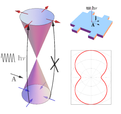
Figure 1: Graphene Hall bar sample irradiated by linearly polarized electromagnetic wave described by vector potential $\mathbf{A}$. Applying a bias voltage leads to an electrical current $\mathbf{j}$ which depends on the photo-induced carrier concentration. The pseudospin orientation of the charge carriers described by Dirac Hamiltonian with the cone-shaped dispersion law shown by arrows is entangled with the particle momentum. The electrons in the valence band absorbing the photon energy $h\nu$ are excited to the conduction band producing the photoconductivity response. The electron-hole excitation rate is zero if the light is polarized along the pseudospins of the excited particles. In contrast, the excitation rate is maximal if the vector potential and pseudospin are perpendicular to each other. Since the pseudospin orientation is coupled with the particle’s momentum the resulting photoconductivity $\sigma_{\mathrm{ph}}$ depends on the angle between $\mathbf{A}$ and $\mathbf{j}$ as shown in the inset. The absolute value of $\sigma_{\mathrm{ph}}$ is estimated in fig. 2.

Graphene membranes are optically transparentNair et al. (2008) as well as highly conductiveBolotin et al. (2008a) even at room temperaturesBolotin et al. (2008b). These two properties being incompatible with each other in conventional materials occur in carbon monolayers quite naturally and make them very promising for optoelectronical applications.Avouris (2010); Bonaccorso et al. (2010) There is, however, another unusual property of carriers in graphene which makes this material even more interesting for optoelectronics. The carriers in graphene display an additional degree of freedom which is often dubbed as the pseudospin but, in fact, is connected to the sublattice index and has nothing to do with the real spin.Castro Neto et al. (2009) We show, that the pseudospin manifests itself in the inter-band optical absorption making the transition probability sensitive to the pseudospin orientations in the initial and final states in a way similar to the real spin selective rules for the inter-band optical transitions in III-V semiconductors. Since the pseudospin is textured in the momentum space, as shown in fig. 1, graphene’s photoconductivity turns out to be anisotropic in the case of the linearly polarised light. The effect seems to be strong enough to find some applications in graphene optoelectronics.

The model described below involves the optical excitation of the valence electrons to the conduction band of intrinsic (i.e. undoped) graphene. The idea is that the effective Hamiltonian describing the interaction between the electromagnetic wave and carriers in graphene inherits the pseudospin-momentum entangled structure from the low energy kinetic term derived within the tight-binding approach.Castro Neto et al. (2009) Assuming normal incidence of a linear polarized electromagnetic wave one deduces an electron generation rate which strongly depends on the relative orientation between the electron momentum and the linear polarization plane, see fig. 1. As consequence, the photoconductivity is predicted to be anisotropic resulting in a high on/off ratio as a function of the linear polarization angle. We note that the photoconductivity in graphene has been also theoretically investigated in recent works,Vasko and Ryzhii (2008); Romanets and Vasko (2010) not analyzing its anisotropy. Moreover, the photoconductivity studied in this work should not be confused with the photocurrents predicted Syzranov et al. (2008); Oka and Aoki (2009); Entin et al. (2010); Mai et al. (2011) and measured Xia et al. (2009); Xu et al. (2010); Park et al. (2009); Karch et al. (2010) in graphene. The photocurrent can be generated without bias voltage applied, whereas the bias is necessary for the photoconductivity measurements. The photoconductivity and photocurrent anisotropy has been also found in the materialsEsayan et al. (1984); Karaman et al. (1983); Gal’perin and Kogan (1969) other than graphene.

II Preliminaries

The two-band effective Hamiltonian for $\pi$-system of graphene near half filling is $H_{0}=\hbar v_{F}(\sigma_{x}k_{x}+\sigma_{y}k_{y})$, where $v_{F}\approx 10^{6}\mathrm{ms^{-1}}$, ${\mathbf{k}}$ is the electron momentum, and $\sigma_{x,y}$ are the Pauli matrices. The Pauli operator $\vec{\sigma}$ represents the pseudospin orientation which is depicted in fig. 1 for the eigenstates of $H_{0}$ given by $\Psi_{\kappa\mathbf{k}}(x,y)=\frac{1}{\sqrt{2}}{\mathrm{e}}^{ik_{x}x+ik_{y}y}\left(1,\kappa{\mathrm{e}}^{i\theta}\right)^{T}$, where $\tan\theta=k_{y}/k_{x}$, and $\kappa=\pm$ denotes the band index, and the energy spectrum of $H_{0}$ is $E_{\kappa k}=\kappa\hbar v_{F}k$.

The interaction between the electromagnetic wave and charge carriers is described by the Hamiltonian $H_{\mathrm{int}}=\frac{ev_{F}}{c}(\sigma_{x}A_{x}+\sigma_{y}A_{y})$ and resembles the pseudospin structure. Assuming the normal incidence and linear polarization of the electromagnetic wave $\mathbf{A}=\mathbf{A}_{0}\exp(-i\omega t+ik_{z}z)$ the golden-rule inter-band transition rate reads

$$I[f_{\kappa\mathbf{k}}]=\sum_{\kappa^{\prime}}\int\frac{d^{2}k^{\prime}L^{2}}{4\pi^{2}}w(\kappa^{\prime}\mathbf{k}^{\prime},\kappa\mathbf{k})(f_{\kappa^{\prime}k^{\prime}}-f_{\kappa k}),$$ (1)

where $f_{\kappa k}$ is the distribution function, and

$$w(\kappa^{\prime}\mathbf{k}^{\prime},\kappa\mathbf{k})=\frac{2\pi}{\hbar}\frac{4\pi^{2}}{L^{2}}\delta(k_{x}-k^{\prime}_{x})\delta(k_{y}-k^{\prime}_{y})\left(\frac{ev_{F}}{c}|A|\right)^{2}$$

$$\times\left[\delta(E_{\kappa^{\prime}k^{\prime}}-E_{\kappa k}-\hbar\omega)+\delta(E_{\kappa^{\prime}k^{\prime}}-E_{\kappa k}+\hbar\omega)\right]$$

$$\times\frac{1+\kappa\kappa^{\prime}\cos(\theta+\theta^{\prime}-2\theta_{\mathrm{pol}})}{2}$$ (2)

is the transition probability. Here $\omega=2\pi\nu$ is the radiation frequency, and $\tan\theta_{\mathrm{pol}}=A_{y}/A_{x}$ is the linear polarization angle. The length $L$ plays a role of the sample size or the laser spot diameter whichever is smaller. Eq. (2) describes the direct inter-band transitions and, thanks to the momentum and energy conservation, naturally includes $\delta$-functions in the first two lines. Most important, however, is the third line which depends on the difference between the linear polarization angle $\theta_{\mathrm{pol}}$ and direction of carrier motion. This dependency disappears in the case of the circular polarization and is crucial for the effect considered below.

III Photoconductivity within the relaxation time approximation

In the following we focus on the electron transport, i.e. $\kappa=+$, and the carriers are excited from the valence to conduction band, as shown in fig. 1. To describe the recombination process we introduce the inelastic relaxation time $\tau_{i}$ which corresponds to the life time of the optically excited states. The steady state distribution function $f^{(1)}_{+k}$ is then obtained by balancing the generation rate (1) and the relaxation rate $f^{(1)}_{+k}/\tau_{i}$ and reads

$$f^{(1)}_{+k}=\frac{2\pi\tau_{i}}{\hbar}\left(\frac{ev_{F}}{c}|A|\right)^{2}\delta(E_{-k}-E_{+k}+\hbar\omega)$$

$$\times\left[f^{(0)}_{-k}-f^{(0)}_{+k}\right]\sin^{2}(\theta-\theta_{\mathrm{pol}}).$$ (3)

We naturally assume that the initial state is the equilibrium one described by the Fermi-Dirac distribution function $f^{(0)}_{\pm k}$. There is no electrical current in the steady state described by the distribution function (3).

The momentum relaxation is assumed to be due to the elastic scattering of carriers on impurities. The average momentum $\hbar\Delta{\mathbf{k}}$ which the electrons gain due to the external electric field ${\mathbf{E}}$ can be estimated as $\hbar\Delta{\mathbf{k}}=e{\mathbf{E}}\tau_{e}$, where $\tau_{e}$ is the elastic momentum relaxation time. For small electric field (linear response) the non-equilibrium term $f^{(2)}_{+k}$ can be obtained by expanding the steady-state function $f^{(1)}_{+(k-\Delta k)}$ with respect to small $\Delta\mathbf{k}$ in up to linear order in $\mathbf{E}$. Recalling $\hbar\mathbf{v}=-\partial_{\Delta\mathbf{k}}E_{+(\mathbf{k}-\Delta\mathbf{k})}|_{\Delta\mathbf{k}=0}$, the non-equilibrium distribution function for photo-excited electrons $f^{(2)}_{+k}$ can be written as

$$f^{(2)}_{+k}=-e\mathbf{E}\mathbf{v}\tau_{e}\frac{\partial f^{(1)}_{+k}}{\partial E_{+k}},\quad\mathbf{v}=v_{F}\left(\begin{array}[]{c}\cos\theta\\ \sin\theta\end{array}\right).$$ (4)

Eq. (4) is valid if and only if $\tau_{i}\gg\tau_{e}$, i. e. optically excited states live much longer than the average time between two subsequent elastic scattering events. This is actually the case in graphene.Avouris (2010); Bonaccorso et al. (2010)

The current density due to the photo-excited electrons can be written as $\mathbf{j}_{\mathrm{ph}}=e\int\frac{d^{2}k}{4\pi^{2}}\mathbf{v}f^{(2)}_{+k}$. This integral can be calculated in polar coordinates with the subsequent substitution $\varepsilon=E_{+k}$ and reads

$$\int d\varepsilon\varepsilon\frac{\partial}{\partial\varepsilon}\left[\delta(\hbar\omega-2\varepsilon)(f^{(0)}_{-\varepsilon}-f^{(0)}_{+\varepsilon})\right]$$

$$=-\frac{1}{2}[f^{(0)}_{-\varepsilon}-f^{(0)}_{+\varepsilon}]_{\varepsilon=\frac{\hbar\omega}{2}}.$$ (5)

The photoconductivity for a given valley/spin channel is then given by

$$\sigma_{\mathrm{ph}}=A_{\mathrm{ph}}\left(\begin{array}[]{cc}2-\cos(2\theta_{\mathrm{pol}})&-\sin(2\theta_{\mathrm{pol}})\\ -\sin(2\theta_{\mathrm{pol}})&2+\cos(2\theta_{\mathrm{pol}})\end{array}\right)$$ (6)

with the amplitude $A_{\mathrm{ph}}$ being

$$A_{\mathrm{ph}}=\frac{e^{2}}{16\hbar^{3}}\tau_{e}\tau_{i}\left(\frac{ev_{F}}{c}|A|\right)^{2}(f^{(0)}_{-\varepsilon}-f^{(0)}_{+\varepsilon})|_{\varepsilon=\frac{\hbar\omega}{2}}.$$ (7)

Rigorous analysis based on the Boltzmann equation written within the relaxation time approximation suggests the same expression for $\sigma_{\mathrm{ph}}$ but both $\tau_{i}$ and $\tau_{e}$ must be substituted by the total relaxation time $\tau^{-1}=\tau_{e}^{-1}+\tau_{i}^{-1}+...$. The effect of anisotropy predicted here does not depend on $\tau$ anyway. Indeed, diagonalizing the matrix (6), the photoconductivity $\sigma_{\mathrm{ph}}^{\parallel}=A_{\mathrm{ph}}$ parallel to the light polarization plane turns out to be $3$ times smaller than the perpendicular one $\sigma_{\mathrm{ph}}^{\perp}=3A_{\mathrm{ph}}$, i.e. the photoconductivity is highly anisotropic, but the anisotropy itself is independent of $\tau$’s. Thus, changing the linear polarization angle from $0$ to $2\pi$ one can observe two minima (and two maxima) in the current flow, as depicted in the inset of fig. 1. These double extrema are a key signature of the effect predicted.

IV Discussion and conclusion

Let us discuss the conditions necessary to observe the anisotropic photoconductivity given by eq. (6) and shown in fig. 1. As it is clear from the analysis given in the previous section the relative anisotropy does not depend on the relaxation times because the relaxation processes reduce the overall photoconductivity, not only its anisotropic part. The physical reason why the anisotropy does not vanish due to the momentum relaxation is the very fact that the anisotropic non-equilibrium distribution relaxes as fast as its isotropic contribution does. We believe therefore that the anisotropy can be detected easily as long as the photoconductivity response is large itself.

To observe the photoconductivity the chemical potential $\mu$ in graphene should be smaller than one-half of the excitation energy $\hbar\omega/2$ enabling direct excitations from the valence band. Assuming THz radiation, as used in the work by Karch et al., Karch et al. we arrive at the maximum $\mu$ less than $10\,\mathrm{meV}$. Thus, the unintentional doping in graphene samples used beforeKarch et al. should be reduced by almost of two orders of magnitude. The temperature can also affect the effect even if the sample is perfectly neutral by reducing the photoconductivity by a factor of the order of $\hbar\omega/2T$ at zero chemical potential. Thus, room temperature $T=25\,\mathrm{meV}$ seems to be somewhat to high for observing a sufficient signal at a radiation frequency of 1 THz. Moreover, the relaxation times $\tau_{e}$ and $\tau_{i}$ assumed to be constant so far, will in fact also be temperature-dependent. However, one can facilitate the measurement by increasing the overall multiplier proportional to the radiation power, possibly by means of a high power pulsed $\mathrm{NH_{3}}$ laser.Ganichev and Prettl (2006)

In contrast to the photocurrents due to photon dragEntin et al. (2010); Karch et al. (2010, ) the above effect is due to the pseudospin-selective inter-band transitions. The momentum transfer from photons to carriers is not important, and the effect should be observable even at normal incidence of light. The predicted anisotropy is strongest for linearly polarized light source, whereas for circular polarization the transition probability (2) does not depend on the direction of carrier motion, and the photoconductivity anisotropy does not occur. An elliptically polarized light source interpolates between these extreme cases. Moreover, the vanishing anisotropy in the case of circular polarization can be used to separate the effect in question from the other photocurrent contributions.Xia et al. (2009); Xu et al. (2010); Park et al. (2009); Karch et al. (2010, )

It is also interesting that the anisotropy predicted Mai et al. (2011) and observedEchtermeyer recently in the photocurrent through graphene pn-junctions seems to have the same origin as the one predicted here. There is, however, $\pi/2$ off-set in the photocurrent vs. polarisation angle dependency as compared with the one shown in fig. 1. This is probably because “the resulting photocurrent comes mainly from electrons moving nearly parallel to the barrier” Mai et al. (2011), and in order to maximize the concentration of such electrons the polarization plane must be set perpendicular to the pn-junction, i.e. along the photocurrent flow. One can reproduce this $\pi/2$ off-set also within our model by taking into account the dependence on ${\mathbf{k}}$ of the angle $\theta$ appearing in eq. (3) in the driving term of the Boltzmann equation.

As already stated, the eigenvalues of the photoconductivity tensor are predicted to differ by a factor of $3$. In order to estimate the overall magnitude of the photoconductivity compared to other conduction mechanisms, let us compare the residual carrier concentration due to the unintentional doping with the one induced by the inter-band excitation. The former varies from $10^{11}\,\mathrm{cm^{-2}}$ for low mobility flakes on $\mathrm{SiO_{2}}$ to $10^{8}\,\mathrm{cm^{-2}}$ for suspended samples after annealing.Peres (2010) The latter can be estimated as $n_{\mathrm{ph}}=\tau_{i}/(L^{2}\tau_{\mathrm{ph}})$ where $\tau_{\mathrm{ph}}$ relates to the total photo-excitation rate as $1/\tau_{\mathrm{ph}}=\int\frac{d^{2}kL^{2}}{2\pi^{2}}I[f_{+\mathbf{k}}]$. On the other hand $\hbar\omega/\tau_{\mathrm{ph}}$ can also be seen as the radiation energy absorption rate which is nothing else than the absorbed radiation power $W_{a}$. Note, that $W_{a}$ relates to the incident radiation power $W_{i}$ as $W_{a}/W_{i}=\pi\alpha$ (where $\alpha=e^{2}/(\hbar c)$ is the fine structure constant) for a single layer graphene membrane.Nair et al. (2008); Kuzmenko et al. (2008) Thus, $n_{\mathrm{ph}}$ at finite temperature $T\neq 0$ can be estimated as

$$n_{\mathrm{ph}}=0.023\frac{W_{i}\tau_{i}}{L^{2}\hbar\omega}(f^{(0)}_{-\varepsilon}-f^{(0)}_{+\varepsilon})|_{\varepsilon=\frac{\hbar\omega}{2}}.$$ (8)

To be specific we assume that the photoconductivity is generated by a $\mathrm{CH_{3}OH}$ laserKarch et al. with wavelength $118\,\mathrm{\mu m}$ (i.e. $\hbar\omega=10.5\,\mathrm{meV}$) and $W_{i}\simeq 20\,\mathrm{mW}$, and the sample itself is a suspended graphene membrane of the macroscopic size slightly larger than the laser spot diameter of about $1\,\mathrm{mm}$. Assuming $\tau_{i}\simeq 1\,\mathrm{ps}$ Avouris (2010); Bonaccorso et al. (2010) we arrive at $n_{\mathrm{ph}}\sim 2\cdot 10^{7}\,\mathrm{cm^{-2}}$ for $L^{2}\simeq 1\,\mathrm{mm^{2}}$ and $T=0$. This values are comparable to the residual carrier concentration for suspended samples,Peres (2010) thus, the conductivity change in the irradiated graphene should be observable. Note, that $n_{\mathrm{ph}}$ can be substantially increased by utilizing smaller samples and focusing the laser beam to a smaller spot. This requires a smaller radiation wave length (i. e. a higher laser frequency) to avoid diffraction effects. The results are summarized in fig. 2.

Figure 2: The concentration of photoinduced carriers $n_{\mathrm{ph}}$ as a function of temperature at different radiation frequency and sample size. (The latter is assumed to be roughly equal to the laser spot diameter and, therefore, has to be substantially larger than the radiation wavelength to avoid diffraction effects.) The photoconductivity can be estimated as $\sigma_{\mathrm{ph}}=e\mu n_{\mathrm{ph}}$, where $\mu$ is the mobility of carriers. The incident radiation power $W_{i}$ and relaxation time $\tau_{i}$ are $10\,\mathrm{mW}$ and $1\,\mathrm{ps}$ respectively.

The effect proposed above relies on the pseudospin texture shown in fig. 1. This texture remains stable as long as the low energy one-particle Hamiltonian $H_{0}$ holds. At least from a theoretical point of view, the pseudospin texture can be altered by electron-electron interactions which may be important in extremely clean samples.Trushin and Schliemann (2011) This is the only fundamental obstacle for the photoconductivity anisotropy observation which we can see so far.

To conclude, we predict strong anisotropy of the photoconductivity in graphene is presence of the linearly polarized light. To observe the effect, we suggest to use undoped suspended graphene samples which allow the laser beam to excite the substantial number of photo-carriers from the valence band. The cleaner samples are expected to demonstrate the better results. They can be used as transparent detectors for the polarisation of the light passing through.