Probing the Universe’s Tilt with the Cosmic Infrared Background Dipole

Abstract

Conventional interpretation of the observed cosmic microwave background (CMB) dipole is that all of it is produced by local peculiar motions. Alternative explanations requiring part of the dipole to be primordial have received support from measurements of large-scale bulk flows. A test of the two hypothesis is whether other cosmic dipoles produced by collapsed structures later than last scattering coincide with the CMB dipole. One background is the cosmic infrared background (CIB) whose absolute spectrum was measured to $\sim 30\%$ by the COBE satellite. Over the 100 to 500 $\mu$m wavelength range its spectral energy distribution can provide a probe of its alignment with CMB. This is tested with the COBE FIRAS dataset which is available for such a measurement because of its low noise and frequency resolution important for Galaxy subtraction. Although the FIRAS instrument noise is in principle low enough to determine the CIB dipole, the Galactic foreground is sufficiently close spectrally to keep the CIB dipole hidden. A similar analysis is performed with DIRBE, which - because of the limited frequency coverage - provides a poorer a dataset. We discuss strategies for measuring the CIB dipole with future instruments to probe the tilt and apply it to the Planck, Herschel and the proposed Pixie missions. We demonstrate that a future FIRAS-like instrument with instrument noise a factor of $\sim 10$ lower than FIRAS would make a statistically significant measurement of the CIB dipole. We find that the Planck and Herschel data sets will not allow a robust CIB dipole measurement. The Pixie instrument promises a determination of the CIB dipole and its alignment with either the CMB dipole or the dipole galaxy acceleration vector.

1. Introduction

Due to their origins, the various cosmic backgrounds provide important information about different aspects of the Universe’s structure and evolution. The adiabatic component of the cosmic microwave background (CMB), being a leftover from the Big Bang, is coupled to the overall structure of space-time during the last scattering (Turner 1991). On the other hand, the cosmic infrared background (CIB) and the cosmic X-ray background (CXB) are produced by emissions from collapsed structures and trace the later evolution of the universe that took place at relatively low $z$ (see reviews by Kashlinsky 2005 and Boldt 1987 for CIB and CXB respectively).

The dipole anisotropy of the CMB is well established from COBE FIRAS (Fixsen et al.1994a) and DMR (Kogut et al 1993, Bennett et al. 1996) measurements. It has a dipole amplitude of $3.346\pm 0.017$ mK in the direction of $(l,b)_{\rm CMB}=(263.85\pm 0.1,48.25\pm 0.04)^{\circ}$ (Hinshaw et al. 2009). If the entire CMB dipole is kinematic its observed amplitude corresponds to velocity of $V=370$ km/sec. At least a substantial part of it must originate from the local motions of the Sun and the Galaxy, so conventional paradigm has been that all of the CMB dipole can be accounted for by motions within the nearby $30-100$ Mpc neighborhood (see review by Strauss & Willick 1995). This paradigm, where CMB dipole converges within the local neighborhood, has been adopted as standard although several inconsistencies between various datasets emerged from the start (Gunn 1988). A possible, if exotic, alternative has been suggested by Turner (1991, 1992), whereby some of the CMB dipole is primordial and reflects a tilt across the observable Universe generated by an isocurvature mode. Such tilt can be produced by preinflationary remnants pushed very far away by the inflationary expansion (Turner 1991, 1992; Grischuk 1992; Kashlinsky et al.1994). In that case the rest-frames of matter and CMB in the Universe are shifted resulting in the appearance of a net motion of galaxies with respect to the CMB across the entire cosmological horizon. Interestingly, this notion has received strong support from measurements based on the cumulative kinematic Sunyaev-Zeldovich effect (Kashlinsky & Atrio-Barandela 2000) which indicate a net coherent motion (dubbed the ”dark flow”) of a sample of $\sim 1,000$ clusters of galaxies extending to at least $\sim 500~{}h^{-1}$Mpc (Kashlinsky et al 2008, 2009, 2010).

If the Universe is tilted, the rest frames of the CMB and galaxies are shifted and the dipoles of the CMB and CIB/CXB may not coincide. (There must always be at least a partial overlap between the dipoles because they share the local motion by the Sun and the Galaxy). This provides an independent test of the tilt. The situation with CXB based on HEAO measurements is inconclusive although the results are marginally consistent with the CMB dipole (Scharf et al. 2000, Boughn et al. 2002). The far-IR CIB presents another opportunity to test this hypothesis. Aside from testing the alignment of CMB and the dipoles from diffuse backgrounds originating from Galaxy emission, various other independent tests of the dark flow phenomenon have been suggested recently (Itoh et al 2009, Zhang 2010, Kosowsky & Kahniashvili 2010).

The far-IR CIB (Puget et al. 1996, Schlegel et al 1998, Hauser et al. 1998, Fixsen et al. 1998) has been reliably measured, both its amplitude and its spectral-energy distribution. It is produced by emission by cold ($T_{d}\sim 20$ K) dust components in galaxies and most of it seems to originate at early times, $z\gtrsim 1$ (Devlin et al. 2009). Its spectral energy distribution is such that the dipole component produced by local motion is amplified, in relative terms, over that of the CMB (see Sec. 3.2.4 of Kashlinsky 2005). This provides a potential way of isolating the CIB dipole component from the local motion and probing its allignment with that of the CMB.

In this paper we present a test for the alignment of the CMB and CIB dipoles. We do this using the best currently available data for this type of analysis: 1) the COBE FIRAS data which have low enough instrument noise and also, importantly, a good frequency coverage with $\Delta\nu\simeq 14$ GHz from 70 to 2,800 GHz across the anticipated peak of the CIB dipole energy distribution; and 2) DIRBE channel 8-10 datasets which have better angular resolution but limited frequency coverage and wide band-widths of $\Delta\nu/\nu\sim 0.3-0.4$ at full width. In Sec. 2 we discuss the magnitude of the CIB dipole assuming perfect alignment with the CMB dipole, our null hypothesis. Sec. 3 then follows with the FIRAS and DIRBE data analysis. We demonstrate there that these data come to within a factor of a few of the null hypothesis CIB dipole, but the uncertainties of the Galactic modeling prevent more discriminative determination. In Sec. 5 we discuss details of a hypothetical experiment that can resolve Galactic contribution better and allow a more unambiguous measurement. Specifically, we examine the prospects of the measurement using the Planck, Herschel and prospective Pixie missions and discuss their potential for measuring the CIB dipole down to the required accuracy.

2. Motivation

The measurements at far-IR ($100~{}\mu{\rm m}\lesssim\lambda\lesssim 1000~{}\mu{\rm m}$) using COBE FIRAS (Puget et al 1996, Fixsen et al 1998) and DIRBE (Hauser et al. 1998, Schlegel et al. 1998) data resulted in consistent detections of the CIB. The FIRAS-based measurements show that the resultant CIB at frequency $\nu$ is well approximated with (Fixsen et al. 1998):

$$I_{\nu}^{\rm CIB}=A(\frac{\nu}{\nu_{0}})^{\beta}B_{\nu}(T_{d})$$ (1)

where $A=(1.3\pm 0.4)\times 10^{-5},\beta=0.64\pm 0.12,T_{d}=18.5\pm 1.2$K, $\nu_{0}=$ 3 THz and $B_{\nu}(T)$ is the Planck function. (The uncertainties in this fit approximation are correlated.)

The motion at velocity $V$ with respect to the CIB would induce a CIB dipole of $\delta I_{\nu}/I_{\nu}=(3-\alpha_{\nu})(V/c)\cos\theta$ with $\theta$ being the angle to the apex of the motion and $\alpha_{\nu}=d\ln I_{\nu}/d\ln\nu$. Here we ignore the quadrupole, $O(V^{2}/c^{2})$, and higher contributions resulting from the relativistic Doppler corrections (Peebles & Wilkinson 1968). If the CIB and CMB dipoles are perfectly aligned, the CIB dipole must lie in the direction of $(l,b)_{\rm CMB}$ and have the amplitude of:

$$\delta I_{\nu}^{\rm dipole}=1.23\times 10^{-3}(3-\alpha_{\nu})I_{\nu}$$ (2)

Since the dust temperature $T_{d}\approx 18.5$ K, the CIB does not reach the Rayleigh-Jeans regime, where the spectral index $\alpha_{\nu}\simeq 2$, until $\lambda\gtrsim 400-500~{}\mu$m. This results in the significantly negative spectral index of the CIB over much of the FIRAS and DIRBE probed bands (see. Fig. 1 of Kashlinsky 2005).

Fig. 1 shows the predicted CIB dipole spectrum, using eq. 1 and assuming perfect alignment with the CMB; the dipole must have a peak value of $(3-5)\times 10^{-3}$ MJy/sr at 100-300$~{}\mu$m, or frequencies 1-3 THz. At longer wavelengths the CMB dipole would overwhelm the signal and at $\lambda\lesssim 100~{}\mu$m the CIB dipole decreases, becoming confused with Galactic and zodiacal light emission. In this wavelength window, however, because of the slope of its spectral energy distribution, the dipole in the CIB becomes $\sim 10^{-2}$ of its mean level compared to $\sim 10^{-3}$ for the CMB.

We model the CIB and other components as

$$I_{\nu}(l,b)=I_{\nu}^{\rm CIB}+\delta I_{\nu}^{\rm dipole}\cos\beta+G_{\nu}(l,b)+{\cal N}_{\nu}$$ (3)

where $\beta$ is the angle between $(l,b)$ and $(l,b)_{\rm CMB}$, the mean ($I_{\nu}^{\rm CIB}$) and dipole ($\delta I_{\nu}^{\rm dipole}$) CIB levels are given by eqs. 1,2 respectably, $G_{\nu}$ is the Galactic emission and ${\cal N}_{\nu}$ is the noise component at frequency $\nu$. This expression, coupled with eqs.

1,2, presents our null hypothesis in the attempt to constrain the CIB dipole, and the tilt, from the FIRAS data. Note that if all of the CMB dipole comes from peculiar motions, the CIB dipole amplitude, $\delta I_{\nu}^{\rm dipole}$, in this decomposition must be given by eq. 2 and Fig. 1.

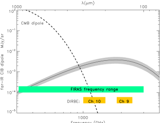
Figure 1.— Shaded region denotes the uncertainty contours of the spectrum the CIB dipole assuming all of the CMB dipole is produced by motion within the local volume; its mean value is shown with the black solid line. Dashes show the measured CMB dipole. The continous frequency coverage of FIRAS and the two lowest frequency (broad) channels of DIRBE are marked.

Two datasets, FIRAS and DIRBE, are currently available for such analysis and, in addition, Planck data will be available shortly. In such measurements Galaxy subtraction is critical and ability to resolve Galatic lines is important in constructing Galaxy templates. The FIRAS instrument with its continuous fine frequency resolution was the main motivation for this investigation. Broad band instruments, such as DIRBE (or Planck) are not capable of supplying accurate Galaxy templates, a point demonstrated earlier by Piat et al (2002) in the context of prospective Planck data analysis. E.g. Cii line at 157$~{}\rm\mu m$ provides a critical template when resolved (as in FIRAS which has bandwidth finer than 1% around that wavelength), but contaminates broad channels such as Channel 9 of DIRBE. In addition it is important to have frequency coverage on both sides of the peak of the predicted energy spectrum of the CIB dipole. This is illustrated in Fig. 1 which shows the continuous frequency coverage of FIRAS and the two broad bands of DIRBE at the lowest frequencies.

3. CIB dipole estimates from FIRAS data.

The FIRAS data are absolutely calibrated, but the precision of the calibration is limited by the small amount of calibration data. Using the FIRAS data in differential mode reduces the calibration errors and greatly reduces the systematic errors as well. A dipole (like the CIB dipole) is differential on the time scale of one orbit. On this scale the FIRAS calibration is much better than the absolute calibration. While the signal to noise is poor at any single frequency, integrated over the full FIRAS spectrum the CIB dipole is expected to have a signal to noise ratio of $\sim$3 with 80% of the statistical weight between .8 and 1.45 THz. The FIRAS data have poor angular resolution ($7^{\circ}$) resulting in a significant Galaxy contribution at the accessible channels of 100 – 1000 $\rm\mu m$. FIRAS frequency resolution is 13.6  GHz allowing continuous coverage between 0.6 and 2.5 THz. The FIRAS instrument resolves the Galactic Cii, Nii and CO lines well enough to separate them from the dust continuum enabling the use of them as templates.

The DIRBE Channels 8,9,10 (nominal wavelengths of 100, 140 and 240 $\rm\mu m$) data probe the peak of the CIB spectrum, and have significantly better angular resolution of $0.7^{\circ}$, but their filters are broad with $\Delta\nu/\nu\sim 0.3-0.4$ and have substantial levels of noise which is even higher in Channel 9.

There are several difficulties in extracting the dipole of the CIB. First the CIB is substantially smaller than the CMB which results in a significantly fainter dipole. Perhaps even more important, the CIB spectrum is much like the Galactic spectrum since the former includes all dusty galaxies with dust properties similar to those in the Milky Way. This limits the usefulness of spectral filters in separating the CIB produced by sources near $z\sim 0$ from the local Galactic signal. Finally, the uncertainties of the FIRAS data, both the raw noise and the systematic errors, rise significantly at higher frequencies.

In this section we present the results of CIB dipole analysis from the FIRAS and DIRBE maps in Galactic coordinates. In this coordinate system, $X$ points in the direction of the center of the Galaxy, $Z$ points in the direction of the Galactic North pole and $Y$ is perpendicular to $X$ and $Z$. Since the solar system is moving faster in its orbit around the Galaxy (presumably it will be moving slower in 100 million years or so) Y points upwind in the interstellar medium. The amplitude of this dipole should be that of figure 1 and the direction should match the direction of the CMB dipole if both dipoles are due to the motion of the Sun or the dipoles in each direction $(X,Y,Z)$ should match.

3.1. Templates

One method of foreground subtraction is the use of templates. Templates are powerful because the FIRAS full sky maps have 6,063 pixels so many templates can be used while using only a small fraction of the number of degrees of freedom available. Since the cost of adding an extra template is relatively low, we use many templates.

The key with templates is that they must be attached to the Galaxy. Using templates that are not attached to the Galaxy runs the risk of removing the dipole along with the Galactic signal. Next we will discuss several templates. These templates can be seen in figure 1 of Fixsen (2009). Except for the zodiacal model all of the templates look approximately alike.

i. One foreground at more than 3 THz is the emission from the solar system zodiacal dust. We use the zodiacal model from the DIRBE team (Kelsall et al. 1998) as a template for this emission.

ii. The Cii emission from the FIRAS maps (Fixsen et al. 1999) has several advantages. The data is already matched in beam shape. Since the Cii line from distant galaxies will be redshifted the Cii template is fixed to the local frame (even if it might excise nearby galaxies as well as the Milky Way). Kogut et al. (2009) note that the square root of the Cii emission tracks emission better than the Cii itself. Here both are used.

iii. The 408 MHz map (Haslam 1981) is often used as a tracer of synchrotron radiation. The CIB is dominated by dust with a peak emission at $\sim 1.5$ THz. At these frequencies, synchrotron emission is insignificant. Furthermore there is significant extragalactic radio emission (Fixsen et al. 2010) so there could be a significant radio dipole. Thus the 408 MHz radio map needs to be treated with care. Still the North Galactic Spur is clearer in the radio than with other templates and the Spur is clearly attached to our own Galaxy. Perhaps there are subtle differences in the dust associated with this region as well. The 408 MHz map needs to be convolved with the FIRAS beam to be used as a template. An estimate of the extragalactic background is subtracted from the 408 MHz map. The major effect of the background subtraction is to reduce the coupling to uniform template. As a uniform background is nearly orthogonal to a dipole.

iv. Hydrogen emission, Hi, should be an ideal tracer of material in the Galaxy. However in places this line becomes optically thick and so suffers from self absorption. One way to mitigate this problem is to include the square of the Hi as well. The Hi from Stark et al. (1992) is convolved with the FIRAS beam to form a template along with map squared.

v. Often the Galaxy is considered as a disk. In this model the emission is expected to be distributed as csc$|b|$. Such modeling has been successfully applied to the DIRBE data isolating CIB fluctuations in the near-IR, but leading to only upper limits at wavelengths longer than $\sim 10~{}\mu$m (Kashlinsky & Odenwald 2000). The model has intrinsic difficulties on the Galactic plane. However, the Galactic plane is too complicated to realistically model anyway, so the csc$|b|$ template can be used and the divergence at $b=0$ is ignored.

vi. The Nii emission from FIRAS and the Al²⁶ emission map (Diehl et al. 1995) also must be local, so although they are not nearly as good tracers of the Galaxy as Cii, they are included as templates.

vii. The DIRBE team also generated a diffuse stellar map to model the starlight. The model is clearly attached to the Galaxy and one would certainly expect that other emission is related to starlight, so this model is also included.

The cosmological background is nearly uniform. To model the uniform background (both the CMB and the CIB) a simple template which is 1 everywhere is used. In principle this model should be orthogonal to the dipole and it is nearly so. However the weights for the FIRAS data are not uniform and the various cuts will not necessarily be symmetric so this term will include the absolute offset or monopole. The uniform background is also convenient in that it provides a model of the CIB that can be used to compare to any observed dipole.

To model a general dipole, we use a set of three orthogonal dipoles $(X,Y,Z)$ in Galactic coordinates defined above. For each of these the dipole is modeled as cos $\phi$ where $\phi$ is the angle between the pixel and the direction of the dipole. Any other coordinates would work as well but this set is convenient and there is clearly a hierarchy of expectations of contamination. That is, the $X$ dipole is most likely to be contaminated as it is sensitive to the differences between the inner Galaxy and the outer Galaxy, where there are clearly observed differences in temperature and composition. The $Y$ dipole is sensitive to the upwind and downwind differences in Galactic radiation. The $Z$ dipole is sensitive to difference between the north and south hemispheres of the Galaxy. There is no intrinsic reason for an asymmetry in this direction although the sun is a bit north of the Galactic equator. Detailed discussion of the relative weight of the errors for various cuts and configurations is given by Atrio-Barandela et al (2010, see e.g. Fig. 4c there).

In other papers the DIRBE band 8, 9, and 10 are used as templates (Fixsen et al. 1996, Fixsen et al. 1997). These bands indeed model the dust very well, however, these data also include the CIB dipole and using them likely would subtract the dipole along with the local dust emission. Still any one of these is a sensitive measure of the likely Galactic contamination. The DIRBE band 10 is used to excise, without bias, the regions of high Galactic emission.

3.2. FIRAS fitting

Given a collection of template maps, $T$, and the FIRAS data, $D$, along with the pixel weights formed into a diagonal matrix, $W$, a least squares fit is made separately at each frequency, resulting in a spectrum, $S$, for each template:

$$S=(T\cdot W\cdot T^{t})^{-1}\cdot T\cdot W\cdot D$$ (4)

No new correlations are introduced in this process but the frequencies are mildly correlated by the previous FIRAS calibration process. Fixsen et al (1999) discuss in detail the line templates used here and their spatial properties.

Since most of the weight for the CIB dipole is in the higher frequency data it is appropriate to use the high frequency weights. All of the Galactic templates have a similar form, so they are highly correlated. This is not a severe problem as long as the matrix is not singular and one is not interested in the spectra associated with the different Galactic templates.

Even with all of these templates the Galactic plane is far too complicated to model in detail. As usual, a cut is made on either the Galactic latitude (ie data is ignored for $|b|<$ cut), or on some measure of Galactic radiation. Here we base our excision on the DIRBE band 10 level. Ideally, one could change the level of cut and find a level where the CIB dipole estimate was insensitive to the level of the cut. In fact for the CMB dipole the direction and amplitude of the fit hardly change going from cutting 10% of the data to cutting 50%.

So we have made fits ranging from no cuts to excising 50% of the data in 5% increments. Cutting beyond 50% of the data runs into three problems. One is that the support of the $X$ and $Y$ dipoles is greatly reduced. A second is that the already highly correlated Galactic models approach singularity as the most emisive and distinctive parts of the Galaxy are systematically excised. Finally the already limited signal to noise is reduced.

Fits can be made with or without each of the 10 foreground templates at each of 11 different Galactic cut levels leading to $11\times 2^{10}=11264$ different fits each with several spectra leading to more than $10^{5}$ spectra. Rather than attempt to present all of these we will attempt to show the best fit.

Clearly fits made including the Galactic plane are still contaminated with foreground emission. Using the CMB dipole as a guide, it appears that excising 30% of the data is approximately the optimum place to cut.

With 70% of the darkest part of the sky, the order of importance of a single template is: 1) the zodiacal template, 2) the $\sqrt{\rm C{\sc II}}$ map, 3) the 408 MHz map, 4) the Hi map, 5) the csc model, 6) the Cii map, 7) the Nii map, 8) the Al²⁶ map, 9) the Hi² map and finally 10) the DIRBE stellar map.

The spectra related to each of the templates can appear peculiar to those unfamiliar with the data and the Galaxy. For example, when including a Cii and an Nii template the corresponding Cii and an Nii spectra contain their corresponding lines as one would expect. The Cii spectrum vaguely resembles the mean Galactic spectrum, but the Nii spectrum is negative at low frequencies and positive at high frequencies. This is because the Nii line is more concentrated near the center of the Galaxy where the average starlight and hence dust temperatures are higher. The negative part of the Nii spectrum is always canceled by the dominate positive Cii spectrum, and the fit uses the Nii to effectively adjust the temperature of the dust.

Since all of the Galactic templates are highly correlated, emission can easily slosh from one to another depending on whether or not other templates are present or whether or not some regions of the sky are included. The high correlation is expected because all of the material, hence the line emission, is concentrated in the Galactic plane. This should help with resolving extragalactic features as most of the high latitude emission is thus local and hence one might expect it to be quite uniform in form if not in intensity.

In this fitting we have not modeled errors in the templates although clearly none of the templates is perfect. Template errors can amplify the “sloshing” that is already present. Small scale errors are likely to just add noise, however large scale errors such as a mismatch in calibration between the north and south calibration of the Hi could dominate the error budget for the $Z$ dipole of the CIB.

Even after subtracting the best fit template spectra there is still significant residual signal. This often appears as a broad dip around 1 THz with a corresponding peak about 2 THz in the residual of fits of the uniform spectrum. This could either be a FIRAS calibration artifact (the absolute spectrum is not calibrated as well as the differential spectrum) or variations in the dust spectrum that are not modeled with the selection of templates used here. The trough and peak are only a sigma or so in amplitude but since this ”feature” extends over many frequency bins it is significant.

Figure 2.— The spectrum associated with the uniform template (the background) with the CMB subtracted. The smooth line is the CIB spectrum from Fixsen et al. 1998. The scatter at high frequencies are from the uncertainty of the FIRAS data.

The smooth CMB dominates the uniform spectrum although a distinct CIB spectrum can be seen at higher frequencies. In fig 2, a single blackbody spectrum has been subtracted from the uniform background spectrum. This is a good model for the CIB. The line is the CIB spectrum from Fixsen et al. 1998, which is a reasonable representation of the data.

Figures 3,4,5 show the 3 derived dipole spectra. The dipole is predicted from the CIB spectrum in figure 2 and the velocity relative to the CMB, $v=370$ km/s toward $(l,b)_{\rm CMB}$, shown as solid lines.

Figure 3.— The spectrum associated with the X dipole template. Solid line is the model of the CMB dipole spectrum.

Figure 4.— The spectrum associated with the Y dipole template. Solid line is the model of the CMB dipole spectrum.

Figure 5.— The spectrum associated with the Z dipole template. Solid line is the model of the CMB dipole spectrum.

Figure 6.— The X dipole spectrum with the X CMB dipole spectrum subtracted. Filled circles show the data with neighboring frequencies averaged to reduce the noise. The smooth line is the expected X CIB dipole.

Figure 7.— The Y dipole spectrum with the Y CMB dipole spectrum subtracted. Filled circles show the data with neighboring frequencies averaged to reduce the noise. Note the scale is different from the X-dipole. The smooth line is the expected Y CIB dipole.

Figure 8.— The Z dipole spectrum with the Z CMB dipole spectrum subtracted. Filled circles show the data with neighboring frequencies averaged to reduce the noise. Note both the horizontal and vertical scales are different from the previous plots. The line is the predicted Z CIB dipole spectrum. Three points of the FIRAS data are above the scale:at 1.92 THz with a dipole value of .36 MJy/sr. DIRBE data Channels 9 and 10 are shown with horizontal bars of width corresponding to the respective band filters.

The nominal fit to a CIB dipole suggests a dipole several times larger than would be expected from the CMB dipole. However the fit is not stable under different cuts and with different templates. So with the FIRAS data we conclude the equivalent velocity of the CIB dipole is less than $7500$ km/s. The uncertainty is completely dominated by systematic errors in subtracting the foreground Galaxy emission.

4. DIRBE

The DIRBE data has higher resolution so the number of potential templates is much larger. However many of the templates (Cii, Nii etc) do not have sufficient resolution to take advantage of the higher resolution of the DIRBE instrument.

Although the DIRBE instrument has 10 bands (frequencies), the mid-range and high frequencies have substantial contamination from the zodiacal dust. In the DIRBE data the mean level of the CIB was detected in just two bands (bands 10 and 9 or 1.25 and 2.1 THz, Hauser et al 1998).

The 100 $\rm\mu m$ (3 THz) band has a nonlinear response. While the effect has largely been corrected any dipole would be suspect. The peak of the CIB dipole should be about 2 THz (150 $\rm\mu m$), so this band is in the Wein part of the spectrum. Also there is still significant residual zodiacal contamination of this band. Thus this is not a good channel to look for the CIB dipole.

The 140 $\rm\mu m$ (2.1 THz ) and 240 $\rm\mu m$ (1.25 THz) bands have many of the same problems as the FIRAS data (not stable under different cuts, high noise) and these lead to two numbers rather than the spectrum of FIRAS. The results of the two channels are respectively 5 and 6 times the expected dipole in the Z direction closely matching the FIRAS results. This shows the agreement between the FIRAS and DIRBE data but the uncertainties are dominated by the same systematics of the foreground subtraction that plague the FIRAS result. Since the same templates were used the systematics are correlated with those of the FIRAS results.

5. Future CIB Dipole Measurements - experimental parameters and prospects

As shown in the preceding sections, the CIB dipole must peak at $\sim 200~{}\rm\mu m$ and must be $\sim 5\times 10^{-3}$ MJy/sr if aligned with the CMB dipole. Although, in principle, the FIRAS noise is low enough to tease out the CIB dipole, in practice, the main impediment to probing the alignment of the CIB and CMB dipoles is confusion with Galactic emission. The physical reason for this is the fact that - with the FIRAS noise levels and without removal of low-$z$ sources - the bulk of the CIB comes from galaxies whose spectral energy distributions are similar to that of the Milky Way. The available templates do not have sufficient fidelity to remove the contaminating foreground signal. With the FIRAS and DIRBE datasets one cannot overcome the Galactic confusion and reliably measure/constrain the CIB dipole, but as we discuss in this section it is possible to successfully make the measurement with the next generation space missions.

Fig. 9 shows the average Galaxy emission compared to the expected CIB dipole spectrum. The residual CMB dipole, assuming the current uncertainties, is shown with a dotted blue line and dominates emission beyond $\sim 500~{}\rm\mu m$. The displayed CIB dipole is shown assuming contributions from all galaxies (black) and from galaxies remaining at $z>0.5,1$ (dashed blue and green lines respectively). For simplicity it was assumed that the CIB is given by eq. 1 and that the apparent dust temperature of the emitters scales as $T_{d}(0)/(1+z)$ and with sources at $z>0.5,1$ contributing 70, 50% of the far-IR CIB at 0.6 THz (500 $\rm\mu m$). The latter normalization is consistent with the BLAST results in the far-IR which indicate that most ($\gtrsim 70\%$) of the CIB at these wavelengths originates in sources at $z\gtrsim 1.2$ (Devlin et al 2009). Thus we can conservatively assume that if we eliminate galaxies to $z=1$ the remaining CIB at 100-300 $\rm\mu m$ would be 50% of the total. Fig. 9 shows that CIB produced by high-$z$ sources becomes progressively more distinguishable in spectrum at increasing $z$. This still leaves the CIB dipole significantly below the foreground Galactic radiation but the spectral difference allows discrimination between the bluer Galactic spectrum and the redder CIB spectrum.

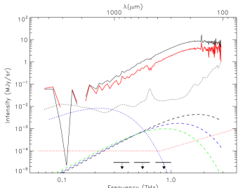
Figure 9.— The solid black line is the average Galaxy spectrum for $|b|>10^{\circ}$ corresponding to the G10 template in the main text. The solid red line is the average Galactic spectrum at $|b|>30^{\circ}$ corresponding to the G30 template in the text. The dashed lines are the expected spectra of the CIB dipole; black, blue, green line correspond to sources at $z\gtrsim 0,0.5,1$ respectively. The dotted blue line shows the CMB dipole residual uncertainty (at 0.017 mK rms uncertainty). The FIRAS noise is shown with the dotted black line. An estimate of the Pixie noise is shown with dotted red line. Three horizontal bars with arrows show the Planck noise limits (below the plot) at its three highest frequency channels.

The currently flying and proposed space missions relevant to the proposed measurement are:

• Planck/HFI has two channels at 545 and 857 GHz (550 and 350 $\rm\mu m$). By 2012, Planck will have mapped the full sky with $\theta_{\rm Planck}=5^{\prime}$ resolution. Fig. 9 marks the highest frequency Planck channels. In principle, the noise levels should allow detection of the CIB dipole. However with only two frequencies and the broad channels with $\Delta\nu/\nu=0.33$ for the HFI instrument (Tauber 2004), convincing separation of the Galactic foreground will be difficult, a point already realized by Piat et al. (2002).

• Herschel/SPIRE covers 250, 350 and 500 $\rm\mu m$ (1200, 857 and 545 GHz) with resolution of order 1 arc minute and FOV $4^{\prime}\times 8^{\prime}$ (Griffin et al. 2008). The detectors are the same spider web detectors as used in the Planck instrument As with Planck a few months of data is enough to get to the noise levels required to look for the CIB dipole. Observing a few widely spaced regions is sufficient, in principle, to detect the CIB dipole. But low frequency noise in the system is likely to limit the calibration stability of the background levels over widely spaced (in time as well as space) observations.

• Pixie is a proposed space mission to observe the full sky with a large throughput (4 cm² sr) Fourier Transform Spectrometer (Kogut et al. 2010). With full sky coverage at angular resolution of $2.5^{\circ}$ and 15 GHz frequency resolution, Pixie will be able to resolve spectral features like the 157 $\rm\mu m$ Cii line to separate the Galactic foreground from the CIB. With a noise floor below $10^{-4}$ MJy/sr per multipole per frequency bin the noise levels are very low to allow a detailed search for CIB anisotropy. The spectral coverage will also allow improvement in estimation of the microwave background dipole. With spectral coverage to 6 THz Pixie will be able to generate new maps for Nii at 122 and 205 $\mu$m, and Oi at 63 $\mu$m as well as generate improved Cii and Nii maps. Fig. 9 shows the estimated noise levels over the frequencies covered by Pixie; they are over two orders of magnitude better than FIRAS.

The contributions to the measured sky dipole from diffuse maps that can confuse the CIB dipole measurement will be from

1. Instrument noise. The dotted lines in Fig. 9 show the FIRAS and Pixie noise levels. Summing over all the FIRAS bands give us S/N$\sim 3$ if the Galaxy were eliminated accurately. The uncertainty in the Galaxy templates costs most of this $S/N$ giving only upper limits on the CIB dipole levels.

2. CMB dipole residual contribution. The CMB dipole is measured with S/N$\gtrsim 1.5\times 10^{4}$ down to the residual uncertainty of $\sigma_{\rm CMB}\simeq 0.017$ mK. The spectrum of this contribution will be given by $B^{\prime}_{\nu}=dB_{\nu}(T_{\rm cmb})/dT_{\rm CMB}$. The dotted blue line in Fig. 9 shows the contribution from the residual CMB dipole with the current measurement uncertainty, but it can be improved with improved measurement.

3. Galactic contribution is described by the available templates and is by far the largest obstacle to the current CIB measurements. This solid black and red lines show the Galactic foregrounds at Galactic cuts $b_{\rm cut}=10^{\circ},30^{\circ}$ respectively; we refer to their templates as G10, G30.

The key requirement is to break the degeneracy between the far-IR CIB energy spectrum and that of the Galaxy over the wavelengths where CIB dipole is near its peak. CMB dipole dominates the long-wavelength emissions, but its energy spectrum is very accurately known and so it can be subtracted making the residual small at wavelengths below $\sim 500~{}\rm\mu m$. If we were able to resolve galaxies out to sufficiently high $z$ and remove them from the maps, the spectrum of the remaining CIB would potentially be sufficiently different to allow robust removal of the Galactic contribution to the dipole. Such experiment should be finely tuned, since at the same time one would need to leave enough sources in the confusion to generate sufficiently measurable levels of the far-IR CIB. Or alternatively, the low-$z$ part of the CIB can be removed together with the Galactic foreground, but that too requires sufficient resolution to remove the Galaxy accurately enough.

Given spectal templates of the CMB and Galaxy contributions ($B^{\prime}_{\nu}$ and $G_{\nu}$ at each channel $\nu$) one can model any measurement with more than three channels, $\nu$, decomposing the measured dipole, ${\cal D}$, into the following terms:

$${\cal D}^{\rm model}_{\nu}={\cal D}_{\nu}^{\rm noise}+aG_{\nu}+bB^{\prime}_{\nu}+d{\cal T}_{\nu}^{\rm CIB}$$ (5)

The last term describes the CIB dipole with the template, $\cal{T}^{\rm CIB}$, given by eq. 1. Given the templates, one can evaluate the CIB dipole after marginalizing over $a$ and $b$ and summing over all the available channels. This is achieved by minimizing $\chi^{2}=\sum_{\nu}({\cal D}^{\rm sky}_{\nu}-{\cal D}^{\rm model}_{\nu})^{2}/\sigma_{\nu}^{2}$ with respect to $(a,b,d)$. The solution for $d$ and its uncertainty, $\sigma_{d}$, is then given by standard regression and error propagation and the signal-to-noise of the prospective measurement will be given by $S/N=d/\sigma_{d}$. In evaluating it below we adopt $\sigma_{\nu}$ in $\chi^{2}$ to be given by the noise per multipole shown in Fig. 9. This allows prediction of the S/N of the CIB dipole measurements as follows for each of the three models of foreground galaxy removal in Fig. 9 ($z\gtrsim 0,0.5,1$ - dashed black, blue, green lines):

• FIRAS. Substituting the parameters for the FIRAS data and the G30 template we obtain after summing over all the FIRAS channels S/N$\simeq 0.13$ for the CIB template of eq. 1. This is what we have actually measured. Equation (5) shows that in order make a significant mea- surement with a future FIRAS-like instrument with the same frequency coverage, the instrument noise must be an order of magnitude below the FIRAS data noise.

• Planck/Herchel. These would not lead to good measurements given that one needs to resolve three parameters ($a,b,d$) from the 2-3 (wide) frequency bands. This can already be seen from the levels of CMB residual dipole in Fig. 9.

• Pixie. Substituting the Pixie parameters, using the G30 model template, we get S/N$\simeq 34,49,46$ for the CIB dipoles given by the dashed black, blue, green lines in Fig. 9. The S/N increases if one eliminates galaxies up to $z\simeq 0.5$ and then starts dropping again because the level of the CIB decreases too. If one uses only the parts of the template with the lines - at wavelengths shorter than $\simeq 160~{}\mu$m, starting with the Cii line - this part of the template contributes about half the signal-to-noise when added in quadrature with S/N$\simeq 22$ for the black line of the CIB dipole (no galaxies removed). If we use the G10 template here too we recover good prospects for such a measurement with S/N$\simeq 25,46,42$ for the three cases of the CIB dipole model. This argues for good prospects of this measurement with Pixie even if not many foreground galaxies are removed from the data.

Importantly, the high S/N for a prospective CIB dipole measurement with Pixie would allow us to also measure the dipole direction with good accuracy. The accuracy of the measured direction for $S/N\gg 1$ would be $\Delta\theta\simeq\sqrt{2}(S/N)^{-1}$radian. Thus for Pixie the accuracy of the CIB dipole direction would be

$$\Delta\theta_{\rm Pixie}\simeq 2^{\circ}\;\frac{40}{(S/N)_{\rm Pixie}}$$ (6)

The current discrepancy between the local acceleration vector direction measured from galaxy surveys and the direction of the CMB dipole is about $\sim 15^{\circ}-20^{\circ}$ (Erdogdu et al 2006, see also Gunn 1988 for discussion of prior measurements) presenting a challenge for the purely kinematic interpretation of the CMB dipole. Thus the Pixie measurement can settle the meaning of that discrepancy as the CIB is expected to be aligned with the true direction of the local motion.

6. Conclusions

We have shown that, because of its spectral energy distribution, the far-IR CIB can provide information on the convergence and the origin of the CMB dipole. To test this the analysis has been applied to the best available current datasets: COBE FIRAS and DIRBE. The main limitation with FIRAS data is accurate modeling of Galactic contamination because low-$z$ galaxies are similar in far-IR emission to the Galactic dust and cannot be removed from the maps because of insufficient angular resolution. Although the Galactic foreground has prevented us from making a positive detection of the CIB dipole, the limit already approaches the expected value. Either a modest improvement in templates (such as a better Cii map) or in measurement accuracy could allow a more definitive measurement. The Planck/Herschel data and, particularly, the proposed Pixie mission data could provide the additional leverage to uncover the CIB dipole and probe its alignment with that of the CMB.

References

- (1)
- (2) Atrio-Barandela, F. et al 2010, ApJ, 719, 77
- (3)
- (4) Hinshaw G et al.2009, ApJS 180, 225
- (5)
- (6) Bennett C et al.1996, ApJL, 464, L1
- (7)
- (8) Boldt E 1987, Phys Rep, 146, 215
- (9)
- (10) Boughn, S., Crittenden, R.G. & Koehrsen, G. P. 2002, ApJ, 580, 672
- (11)
- (12) Devlin, M.J. et al 2009, Nature, 458, 737
- (13)
- (14) Diehl R et al., 1995, A&A, 298, 445
- (15)
- (16) Erdogdu, P. et al 2006, MNRAS, 368, 1515
- (17)
- (18) Fixsen DJ et al., 1994a, ApJ, 420, 445
- (19)
- (20) Fixsen DJ et al., 1996, ApJ, 473, 576
- (21)
- (22) Fixsen DJ et al., 1997, ApJ, 486, 623
- (23)
- (24) Fixsen DJ et al., 1998, ApJ, 508, 123
- (25)
- (26) Fixsen DJ, Bennett CL & Mather JC, 1999, ApJ, 526, 207
- (27)
- (28) Fixsen DJ et al., 2009, ApJ, submitted
- (29)
- (30) Fixsen DJ, 2009, ApJ, 707, 916
- (31)
- (32) Griffin M et al., 2008, Proc SPIE 7010E, 4
- (33)
- (34) Grischuk L. 1992, Phys. Rev. D 45, 4717
- (35)
- (36) Gunn, J. 1988, In “The extragalactic distance scale”, ASP 100th Anniversary Symposium, p. 344.
- (37)
- (38) Haslam CGT, et al., 1981, A&A, 100, 209
- (39)
- (40) Hauser MG et al., 1998, ApJ, 508, 44
- (41)
- (42) Hinshaw G et al., 2009, ApJS, 180, 225
- (43)
- (44) Itoh, Y. et al 2009, arxiv:0912.1460
- (45)
- (46) Kashlinsky, A. & Atrio-Barandela, F. 2000, Astrophys. J., 536, L67
- (47)
- (48) Kashlinsky, A., Atrio-Barandela, F., Kocevski, D. & Ebeling, H. 2008, ApJ, 686, L49
- (49)
- (50) Kashlinsky, A., Atrio-Barandela, F., Kocevski, D. & Ebeling, H. 2009, ApJ, 691, 1479
- (51)
- (52) Kashlinsky, A., Atrio-Barandela, F., Ebeling, H., Edge, A., & Kocevski, D. 2010, ApJ, 712, L81
- (53)
- (54) Kashlinsky, A., Tkachev, I. & Frieman, J. 1994, Phys. Rev. Letters, 73, 1582
- (55)
- (56) Kashlinsky, A. & Odenwald, S. 2000, ApJ, 528, 74
- (57)
- (58) Kashlinsky A. 2005, Physics Reports, 409, 361
- (59)
- (60) Kelsall et al., 1998, ApJ, 508, 25
- (61)
- (62) Kogut A et al., 1993, ApJ, 419, 1
- (63)
- (64) Kogut A et al., 2009, ApJ, submitted
- (65)
- (66) Kogut A et al., 2010, in preparation
- (67)
- (68) Kosowsky, A. & Kahniashvili, T. 2010, Phys Rev Lett., submitted (arxiv:1010.4543)
- (69)
- (70) Peebles, J. E., & Wilkinson, D. T. 1968, Phys. Rev., 174, 2168
- (71)
- (72) Priat, M et al., 2002, A&A, 393, 359
- (73)
- (74) Puget, JL et al., 1996, A&A, 308, L5
- (75)
- (76) Scharf, C. et al 2000, ApJ, 544, 49
- (77)
- (78) Stark, A. et al 1992, ApJS, 79, 77
- (79)
- (80) Schlegel, D.J., Finkbeiner, D.P., Davis, M. 1998, ApJ, 500, 525
- (81)
- (82) Strauss MA & Willick JA, 1995, Physics Reports, 261,271
- (83)
- (84) Tauber, J. 2004, Adv. Space Research, 34, 491
- (85)
- (86) Turner M. 1991, Phys Rev D, 44, 3737
- (87)
- (88) Turner M. 1992, General Relativity and Gravitation, 24, 1
- (89)
- (90) Zhang, P. 2010, MNRAS (Letters), 407, L36. arXiv:1004.0990
- (91)