Y-system for $\mathbb{Z}_{S}$ Orbifolds of $\mathcal{N}$ = 4 SYM

Abstract:

We propose a twisted Y-system for the calculation of leading wrapping corrections to physical states of general $\mathbb{Z}_{S}$ orbifold projections of $\mathcal{N}=4$ super Yang-Mills theory. Agreement with available thermodynamical Bethe Ansatz results is achieved in the non supersymmetric case. Various examples of new computations, including other supersymmetric orbifolds are illustrated.

1 Introduction

The study of orbifolds of AdS/CFT duality is a very interesting topic where supersymmetry can be broken in a mild way, namely by boundary conditions [1, 2]. Planar integrability is known to be preserved [3, 4] and the study of ubiquitous wrapping corrections [5] is clearly interesting.

The standard setup is that of a stack of $N$ D3-branes located on the fixed point of the orbifold $\mathbb{C}^{3}/\Gamma$. By gravitational backreaction, the near-horizon geometry is $AdS_{5}\times(S^{5}/\Gamma)$, where the discrete group $\Gamma$ is a finite subgroup of $SO(6)$, the isometry group of $S^{5}$. AdS/CFT predicts duality between type II string and a particular orbifold projection of four dimensional $\mathcal{N}=4$ SYM, where the action of $\Gamma$ is extended on $SU(4)$, the spin cover of $SO(6)$. The center of $SU(4)$ is $\mathbb{Z}_{4}$ and there is a $\mathbb{Z}_{2}\equiv\widetilde{\mathbb{Z}}_{2}\subset\mathbb{Z}_{4}$ such that $SU(4)/\widetilde{\mathbb{Z}}_{2}=SO(6)$. The group $\Gamma$, as a subgroup of $SU(4)$ does not contain the non trivial element of $\widetilde{\mathbb{Z}}_{2}$. Thus $\Gamma/\widetilde{\mathbb{Z}}_{2}\equiv\Gamma$ [1, 2].

Remarkably, since $AdS_{5}$ is untouched, one expects large $N$ (or better said, planar) conformal invariance. Actually, the construction is more general and can be applied in the reverse, starting with a generic $\Gamma\subset SU(4)$. In this case, one can obtain type 0 string theory if $\Gamma$ does not project trivially on $SO(6)$, i.e. $\Gamma/\widetilde{\mathbb{Z}}_{2}\neq\Gamma$ [6, 7, 8, 9].

In this paper, we propose a method to compute the leading wrapping finite size corrections to the abelian $\mathbb{Z}_{S}$ orbifolds of the $AdS_{5}\times S^{5}$ superstring [3]. The most powerful and general approach to the evaluation of these corrections is the mirror thermodynamic Bethe Ansatz (TBA) developed for the unorbifoldized theory in [10] and deeply tested in [11], mainly in the theoretical laboratory of $\mathfrak{sl}(2)$ states. The associated Y-system has been conjectured in [12] based on symmetry arguments and educated guesses about the analyticity and asymptotic properties of the Y-functions.

The same methods can be extended to study finite-size corrections in theories which are closely related to $\mathcal{N}=4$ SYM by AdS/CFT duality. These are obtained as ($\beta$-) deformations or quotients of the $AdS_{5}\times S^{5}$ string background. The crucial ingredient to recover the twisted Bethe equations of [13] are the associated deformed transfer matrices, which can be obtained by twisting the undeformed transfer matrix [14], or by twisting the S-matrix [15]. Successful applications to $\beta$-deformed theories have been presented in [16, 17, 18] at the level of the transfer matrix, and in [15, 19] in the $S$-matrix formalism.

Analogous applications to the case of orbifolds has been presented in [14] and [20], focusing on non-supersymmetric orbifolds which are special cases of the general treatment of [3]. Here, we consider the construction of the Y-system for all cases considered in [3] and follow the approach of [12, 16], thus bypassing the many subtleties of the rigorous TBA treatment or the S-matrix approach. This makes our proposal an educated conjecture which could be hopefully helpful for a more solid investigation. The main point is that the orbifold projection breaks supersymmetry by boundary conditions on the string side. This means that the powerful symmetry constraints of the untwisted case are inherited in the bulk. In more simple terms, the Y-system can be conjectured to be associated with the same Hirota dynamics where the twisting parameters enter as rigid deformation parameters of polynomial solutions.

In the non-supersymmetric case , we agree with the results of [14, 20] and present a reciprocity respecting closed formula for the leading wrapping correction to twist-3 operators in the orbifoldized $\mathfrak{sl}(2)$ subsector. For other orbifolds, we illustrate various examples where the calculation of leading wrapping corrections to physical states is definitely feasible as well as rather simple.

The plan of the paper is the following. In Sec.(2), we review the main features of orbifolds of AdS/CFT duality. In Sec.(3), we present the asymptotic Bethe Ansatz for orbifolds. In Sec.(4), we illustrate the proposed twisted Y-system. Finally, in Sec.(5) , we report various applications and checks.

2 Orbifolds of AdS/CFT duality

In orbifoldized AdS/CFT duality, we start from $AdS_{5}\times S^{5}$ and quotient $S^{5}$ by a discrete isometry subgroup $\Gamma$ of $SO(6)$, or more generally of the spin cover $SU(4)$ as mentioned in the introduction. On the gauge theory side, we deal with what is called an orbifold projection (see for instance [2]). The initial $N$ D3-branes have $|\Gamma|\,N$ images. Thus, it is convenient to split the gauge index of $U(|\Gamma|\,N)$ as the pair $(i,h)$, with $i=1,\dots,N$, and $h\in\Gamma$. The action of the orbifold group is simply $g:(i,h)\mapsto(i,g\,h).$ For example, if $\Gamma=\mathbb{Z}_{S}$, the index $I=1,\dots,SN$ is split into $S$ blocks of length $N$ and the action of $\mathbb{Z}_{S}$ is simply addition modulo $S$. The Lagrangian of the orbifold projection is the same as in $\mathcal{N}=4$, with projected (under $P_{\Gamma}=\frac{1}{|\Gamma|}\sum_{g\in\Gamma}g$) vector and chiral superfields .The group action on gauge indices spans the regular representation $\rho_{\rm reg}$. The vector and chiral superfields transform as

$$\mathcal{A}\sim\rho_{\rm reg}^{\oplus N}\otimes\overline{\rho}_{\rm reg}^{\oplus N},\qquad\Phi\sim\rho_{R}\otimes\rho_{\rm reg}^{\oplus N}\otimes\overline{\rho}_{\rm reg}^{\oplus N},$$ (1)

where $\rho_{R}$ is a 3-dimensional representation acting on the chiral field index $a=1,2,3$.

After projection, it is easy to identify the invariant gauge fields and the associated orbifold gauge group. To this aim, one decomposes the regular representation as

$$\rho_{\rm reg}=\bigoplus_{\lambda}\rho_{\lambda}^{\oplus N_{\lambda}},\qquad N_{\lambda}=\dim\rho_{\lambda},$$ (2)

where $\rho_{\lambda}$ are the irreducible representations of $\Gamma$. From the invariance condition $\mathcal{A}=\rho_{\rm reg}(g)\,\mathcal{A}\,\rho_{\rm reg}^{-1}(g),$ we deduce that also $\mathcal{A}$ is block diagonal and, as a consequence, the orbifold gauge group is $G_{\rm orb}=\bigotimes_{\lambda}U(NN_{\lambda}).$ In other words, we simply isolate the singlet representation in

$$\rho_{\rm reg}^{\oplus N}\otimes\overline{\rho}_{\rm reg}^{\oplus N}=\bigoplus_{\lambda,\lambda^{\prime}}\rho_{\lambda}\otimes\overline{\rho}_{\lambda^{\prime}}\otimes\mathbb{C}^{NN_{\lambda}}\otimes(\mathbb{C}^{*})^{NN_{\lambda^{\prime}}}=\left[\bigoplus_{\lambda}\rho_{0}\otimes\mathbb{C}^{NN_{\lambda}}\otimes(\mathbb{C}^{*})^{NN_{\lambda}}\right]\oplus\cdots.$$ (3)

The complexified coupling $\tau=\frac{4\pi i}{g^{2}}+\frac{\theta}{2\pi}$ breaks down to the couplings $\tau_{\lambda}=\frac{N_{\lambda}}{|\Gamma|}\,\tau,$ associated with the factors $U(NN_{\lambda})$.

The invariant matter can be computed in a similar way. We have initially Weyl fermions $\Psi^{\alpha}_{IJ}$ in the adjoint of the gauge group with $\alpha$ in the $\mathbf{4}$ of $SU(4)$, and scalars $\Phi^{m}_{IJ}$ in the adjoint of the gauge group with $m$ in the $\mathbf{6}$ of $SO(6)$ which is $(\mathbf{4}\otimes\mathbf{4})_{\rm A}$ of $SU(4)$. For any representation $R$ we define the branching coefficients $a^{R}_{\lambda\lambda^{\prime}}$ from $\rho_{R}\otimes\rho_{\lambda}=\bigoplus_{\lambda^{\prime}}a^{R}_{\lambda\lambda^{\prime}}\,\rho_{\lambda^{\prime}}.$ Then, the singlets surviving projections are obtained from the relation

$$\rho_{R}\otimes\rho_{\rm reg}^{\oplus N}\otimes\overline{\rho}_{\rm reg}^{\oplus N}=\left[\bigoplus_{\lambda,\lambda^{\prime}}a^{R}_{\lambda\lambda^{\prime}}\,\rho_{0}\otimes\mathbb{C}^{NN_{\lambda}}\otimes(\mathbb{C}^{*})^{NN_{\lambda^{\prime}}}\right]\oplus\cdots.$$ (4)

Thus, we have $a^{R}_{\lambda\lambda^{\prime}}$ fields transforming in the $(NN_{\lambda},\overline{NN_{\lambda^{\prime}}})$ bifundamental representation of the subgroup pair $U(NN_{\lambda})\times U(NN_{\lambda^{\prime}})\subset G_{\rm orb}.$ This information can be encoded in a quiver diagram [22] where each representation $\rho_{\lambda}$ is associated with a node, and we draw $a^{R}_{\lambda\lambda^{\prime}}$ directed arrows for each associated fields. It can be shown that there is a Yukawa coupling for all $(\mbox{fermion})^{2}\cdot\mbox{boson}$ triangles, and a quartic coupling for all $(\mbox{\rm boson})^{4}$ squares.

The residual supersymmetry is also easily identified. Let $SU(2)\subset SU(3)\subset SU(4)$ be the standard embedding. It can be shown that if $\Gamma\subset SU(3)$, then the residual supersymmetry of the orbifold projected theory is $\mathcal{N}=1$. If $\Gamma\subset SU(2)$, then it is $\mathcal{N}=2$. The multiplet identification goes as follows. In the $\mathcal{N}=1$ case, we can reduce the $\bf{4}$ of $SU(4)$ under $SU(3)$ as ${\bf 4}={\bf 3}\oplus{\bf 1}$. The ${\bf 3}$ is a triplet of Weyl spinors. The singlet is the gaugino. The scalars organize with respect to $SU(3)$ as

$$6=[(3\oplus 1)\otimes(3\oplus 1)]_{\rm A}=(3\otimes 3)_{\rm A}\oplus(3\otimes 1+1\otimes 3)_{\rm A}=\overline{3}\oplus 3.$$ (5)

Thus, we have a triplet and an antitriplet of real scalars. With the Weyl fermions, they build up three chiral superfields, as is known to happen when reducing the $\mathcal{N}=4$ hypermultiplet to $\mathcal{N}=1$. The gaugino pairs with the gauge potential build a $\mathcal{N}=1$ vector superfield.

In the $\mathcal{N}=2$ case, we can reduce the ${\bf 4}$ of $SU(4)$ under $SU(2)$ as ${\bf 4}={\bf 2}\oplus{1}\oplus{\bf 1^{\prime}}.$ The ${\bf 2}$ is a doublet of Weyl spinors. The singlets are two gauginos. The scalars organize with respect to $SU(2)$ as

$$6 = [(2\oplus 1\oplus 1^{\prime})\otimes(2\oplus 1\oplus 1^{\prime})]_{\rm A}=(2\otimes 2)_{\rm A}\oplus 2(2\otimes 1+1\otimes 2)_{\rm A}\oplus(1\otimes 1^{\prime})_{\rm A}=$$ (6)

$$= 1\oplus 2\cdot{\bf 2}\oplus 1^{\prime}.$$

Thus, we have two doublets of real scalars that combine with the doublet of Weyl fermions to build two chiral superfields. One gaugino pairs with the gauge fields and the other with the remaining two scalars in an additional $SU(2)$-invariant chiral superfield. This is indeed a $\mathcal{N}=2$ hypermultiplet.

3 Asymptotic twisted Bethe Ansatz

The asymptotic Bethe Ansatz for $\mathbb{Z}_{S}$ orbifold of planar $\mathcal{N}=4$ SYM has been derived in [3]. Here, we briefly review its main features as a preparation for the construction of the Y-system.

The group $\mathbb{Z}_{S}$ has $S$ (one-dimensional) irreducible representations where the cyclic element $g$ such that $g^{S}=1$ is represented as

$$\rho_{n}(g)=\omega^{n},\qquad n=0,\dots,S-1,\qquad\omega=e^{\frac{2\pi\,i}{S}\,n}.$$ (7)

The orbifold is thus a quiver theory with $S$ nodes and gauge group $U(N)^{\otimes S}$. The product of representations is of course simply

$$\rho_{n}\otimes\rho_{n^{\prime}}=\rho_{n+n^{\prime}\mod S}$$ (8)

In general, we start by representing $g$ on the Weyl fermions, i.e. on the 4 of $SU(4)$. This will take the form

$$g_{\bf 4}=\mbox{diag}(\omega^{n_{i}}),\qquad i=1,\dots,4,\qquad n_{1}+\cdots+n_{4}=0\mod S.$$ (9)

The representation of $g$ on the 6 of $SU(4)$ follows from ${\bf 6}=({\bf 4}\times{\bf 4})_{\rm A}$ . Thus

$${\bf 4}=\bigoplus_{i=1}^{4}\rho_{n_{i}},\qquad{\bf 6}=\mathop{\bigoplus_{i=1}^{4}}_{i<j}\rho_{n_{i}+n_{j}}.$$ (10)

This allows to compute $a^{\bf 4}_{nm}$ and $a^{\bf 6}_{nm}$ and hence the quiver diagram. The amount of residual supersymmetry can be easily recognized as we mentioned in the previous section. This is a somewhat important issue since the leading order at which wrapping effects appear is delayed in perturbation theory by supersymmetry, as it happens in the unorbifoldized $AdS_{5}\times S^{5}$ case.

We parametrize the cyclic element $g_{\bf 4}$ in the fundamental of $SU(4)$ acting on Weyl fermions as

$$g_{\bf 4}=\mbox{diag}(\omega^{-t_{1}},\omega^{t_{1}-t_{2}},\omega^{t_{2}-t_{3}},\omega^{t_{3}}),\qquad\omega=e^{2\pi i/S},$$ (11)

where $S=2,3,\dots$ determines the orbifold order. Fields with definite $SU(4)$ charges obey

$$X=\omega^{s_{X}}\,\rho\,X\,\rho^{-1},$$ (12)

where $\rho$ is the representation of the orbifold action on the gauge indices. This relation can be used to bring all twist matrices together. We are led to consider the operators

$$\mathcal{O}=\mbox{Tr}(\rho^{T}\,\mathcal{W}_{A_{1}}\cdots\mathcal{W}_{A_{L}}),\qquad\mathcal{W}\in\{D^{n}\varphi,D^{n}\psi,D^{n}F\}$$ (13)

where $T=0,\dots,S-1$ labels the twist sector and, for long enough operators, is a conserved quantum number. These operators are non (trivially) vanishing if the sum of twist charges vanishes

$$\sum_{i=1}^{L}s_{A_{i}}=0\mod S.$$ (14)

The asymptotic one-loop Bethe equations, cyclicity condition and twist constraint turn out to be (here $J=7$ and $L$ is the length of the Bethe states)

$$\omega^{T\,s_{j}}\,\left(\frac{u_{j,k}-\frac{i}{2}V_{j}}{u_{j,k}+\frac{i}{2}V_{j}}\right)^{L}\,\mathop{\prod_{j^{\prime}=1}^{J}\prod_{k^{\prime}=1}^{K_{j^{\prime}}}}_{(j,k)\neq(j^{\prime},k^{\prime})}\frac{u_{j,k}-u_{j^{\prime},k^{\prime}}+\frac{i}{2}M_{jj^{\prime}}}{u_{j,k}-u_{j^{\prime},k^{\prime}}-\frac{i}{2}M_{jj^{\prime}}}=1,$$ (15)

$$\omega^{T\,s_{0}}\,\prod_{j=1}^{J}\prod_{k=1}^{K_{j}}\frac{u_{j,k}+\frac{i}{2}V_{j}}{u_{j,k}-\frac{i}{2}V_{j}}=1,$$ (16)

$$\omega^{-L\,s_{0}}\,\prod_{j=1}^{J}\omega^{-K_{j}\,s_{j}}=1.$$ (17)

Here, $M$ is the Cartan matrix of the $\mathfrak{psu}(2,2|4)$ algebra, $V_{j}$ are the weights determining the transformation rules of the associated spin chain, and $\{s_{j}\}_{j=0,\dots,7}$ are twist exponents. Their values for $j>0$ can be computed starting from the oscillator representation of the Dynkin diagram. The value of $s_{0}$ is computed from the vacuum state of the specific Dynkin diagram. The explicit values for the higher form of the Dynkin diagram [23] are shown in Fig. (1).

Figure 1: Values of the twist exponents $\{s_{j}\}$ for the higher Dynkin diagram.

For this Dynkin diagram we have the following Cartan matrix and weights

$$M={\small\left(\begin{array}[]{ccccccc}&1\\ 1&-2&1\\ &1&&-1\\ &&-1&2&-1\\ &&&-1&&1\\ &&&&1&-2&1\\ &&&&&1\end{array}\right)},\quad V_{j}=\delta_{j,4}.$$ (18)

As discussed in [3], the twist exponents do not change when the Bethe equations are replaced by their all-order asymptotic form, including dressing corrections. We shall not need them in explicit form in the following manipulations which can be done at one-loop.

3.1 $\mathfrak{sl}(2)$ grading

In the following, it will be convenient to dualize the fermionic nodes in order to write the Bethe equations in $\mathfrak{sl}(2)$ grading. To this aim, and following standard manipulations, we introduce $\widetilde{K}_{j}$ dual roots at fermionic nodes and associated polynomials $Q_{j}=\prod_{k=1}^{K_{j}}(u-u_{j,k})$, $\widetilde{Q}_{j}=\prod_{k=1}^{\widetilde{K}_{j}}(u-\widetilde{u}_{j,k})$, according to

$$\omega^{T\,s_{1}}\,Q_{2}^{+}-Q_{2}^{-}=(\omega^{T\,s_{1}}-1)\,Q_{1}\,\widetilde{Q}_{1}, \qquad K_{1}+\widetilde{K}_{1}=K_{2},,$$

$$\omega^{T\,s_{3}}\,Q_{2}^{+}Q_{4}^{-}-Q_{2}^{-}Q_{4}^{+}=(\omega^{T\,s_{3}}-1)\,Q_{3}\,\widetilde{Q}_{3}, \qquad K_{3}+\widetilde{K}_{3}=K_{2}+K_{4},$$

$$\omega^{T\,s_{5}}\,Q_{4}^{-}Q_{6}^{+}-Q_{4}^{+}Q_{6}^{-}=(\omega^{T\,s_{5}}-1)\,Q_{5}\,\widetilde{Q}_{5}, \qquad K_{5}+\widetilde{K}_{5}=K_{4}+K_{6},$$

$$\omega^{T\,s_{7}}\,Q_{6}^{+}-Q_{6}^{-}=(\omega^{T\,s_{7}}-1)\,Q_{7}\,\widetilde{Q}_{7}, \qquad K_{7}+\widetilde{K}_{7}=K_{6}.$$ (19)

Again, we stress that these are one-loop relations with simple extension to the all-order deformation. Replacing in the Bethe equations we can rewrite them in the $\mathfrak{sl}(2)$ form as

$$\omega^{T\,\widetilde{s}_{j}}\,\left(\frac{u_{j,k}-\frac{i}{2}V_{j}}{u_{j,k}+\frac{i}{2}V_{j}}\right)^{L}\,\mathop{\prod_{j^{\prime}=1}^{J}\prod_{k^{\prime}=1}^{K_{j^{\prime}}}}_{(j,k)\neq(j^{\prime},k^{\prime})}\frac{u_{j,k}-u_{j^{\prime},k^{\prime}}-\frac{i}{2}M_{jj^{\prime}}}{u_{j,k}-u_{j^{\prime},k^{\prime}}+\frac{i}{2}M_{jj^{\prime}}}=1,$$ (20)

where the dualized twist exponents are

$$\begin{array}[]{|c|c|c|c|c|c|c|}\hline\cr\widetilde{s}_{1}&\widetilde{s}_{2}&\widetilde{s}_{3}&\widetilde{s}_{4}&\widetilde{s}_{5}&\widetilde{s}_{6}&\widetilde{s}_{7}\\ -t_{1}&2t_{1}-t_{2}&t_{2}-t_{1}&0&t_{2}-t_{3}&2t_{3}-t_{2}&-t_{3}\\ \hline\cr\end{array}$$ (21)

The (unaltered) twisted ciclicity and twist constraints read

$$\omega^{T\,s_{0}}\,\prod_{k=1}^{K_{4}}\frac{u_{4,k}+\frac{i}{2}}{u_{4,k}-\frac{i}{2}}=1,$$ (22)

$$L\,s_{0}+\sum_{j=1}^{7}\widetilde{K}_{j}\,\widetilde{s}_{j}=0\mod S.$$ (23)

We remark that $s_{0}$ does not depend on grading, and in the twist constraint, we understand $K_{j}=\widetilde{K}_{j}$ for the bosonic nodes.

4 Twisted Y-system for $\mathbb{Z}_{S}$ orbifolds

The spectrum of relativistic 1+1 dimensional integrable theories has been suggested [24] to be captured by the universal set of functional quadratic Hirota equations taking the form

$$T_{a,s}(u+i/2)\,T_{a,s}(u-i/2)=T_{a+1,s}(u)\,T_{a-1,s}(u)+T_{a,s+1}(u)\,T_{a,s-1}(u)\;.$$ (24)

For the $AdS_{5}\times S^{5}$ superstring theory the system of Hirota equations should be the same, with the functions $T_{a,s}(u)$ being non-zero only inside the infinite T-shaped domain of the ${a,s}$ integer lattice, shown in Fig. (2).

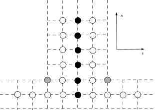
Figure 2: Graphical representation of the Y-system and T-system. Circles correspond to Y-functions. Intersections of grid lines in the T-hook correspond to T-functions.

Physical quantities can be computed by introducing the gauge invariant $Y$-functions

$$Y_{a,s}=\frac{T_{a,s+1}T_{a,s-1}}{T_{a+1,s}T_{a-1,s}}\;\;,$$ (25)

which obey another set of functional equations called the Y-system:

$$\frac{Y_{a,s}^{+}Y_{a,s}^{-}}{Y_{a+1,s}Y_{a-1,s}}=\frac{(1+Y_{a,s+1})(1+Y_{a,s-1})}{(1+Y_{a+1,s})(1+Y_{a-1,s})}\,,$$ (26)

The T- and Y-systems should additionally be supplemented with a particular set of analytical properties imposed on T- and Y-functions. The deep analysis of these properties in the AdS/CFT case is discussed in [10].

The energy and momentum of magnon excitations in the theory are described in terms of $x(u)$, defined by

$$x+\frac{1}{x}=\frac{u}{g},$$ (27)

where the relation between the coupling $g$ and the ’t Hooft coupling $\lambda$ is $\lambda=16\pi^{2}g^{2}$. The mirror and physical branches of this function are defined as

$$x^{\rm ph}(u)=\frac{1}{2}\,\left(\frac{u}{g}+\sqrt{\frac{u}{g}-2}\;\sqrt{\frac{u}{g}+2}\right)\;\;,\;\;x^{\rm mir}(u)=\frac{1}{2}\left(\frac{u}{g}+i\sqrt{4-\frac{u^{2}}{g^{2}}}\right)\,.$$ (28)

The energy and momentum of a bound state with $n$ magnons are 

$$\varepsilon_{n}(u)=n+\frac{2ig}{x^{[+n]}}-\frac{2ig}{x^{[-n]}}\;\;,\;\;p_{n}(u)=\frac{1}{i}\log\frac{x^{[+n]}}{x^{[-n]}}\;.$$ (30)

Finally, the exact energy of a state is given by

$$E=\sum_{j}\varepsilon_{1}^{\rm ph}(u_{4,j})+\delta E\;\;,\;\;\delta E=\sum_{a=1}^{\infty}\int_{-\infty}^{\infty}\frac{du}{2\pi i}\,\,\frac{\partial\varepsilon_{a}^{*}(u)}{\partial u}\log\left(1+Y_{a,0}^{*}(u)\right)\;,$$ (31)

where the rapidities $u_{4,j}$ are fixed by the exact Bethe ansatz equations

$$Y_{1,0}^{\rm ph}(u_{4,j})=-1.$$ (32)

Here, $Y_{a,0}^{*}$ denotes the function $Y_{a,0}$ evaluated at mirror kinematics.

4.1 Twisting and matching

The clever idea of [12] is that, for asymptotically large size $L$, it is possible to solve the $Y$-system explicitly since the massive nodes $Y_{a,0}$ decouple and the Y-system splits into two wings $\mathfrak{su}_{\rm L}(2|2)\oplus\mathfrak{su}_{\rm R}(2|2)$. At weak coupling, the solution found in this way can also be used to compute leading wrapping corrections at fixed finite $L$.

The explicit form of the transfer matrices can be derived from the solutions of the Hirota equation for a domain called L-hook (one half of the T-hook diagram in Fig.(2)) and written in the form of a generating functional [25]. The construction of [26] allows for certain free parameters that have been exploited in [16] to build the transfer matrices for the $\beta$-deformed theory. Here, we shall exploit them to compute the orbifold transfer matrices. Let us introduce the quantities

$$\widetilde{R}^{(\pm)}=\prod_{j=1}^{K_{4}}\frac{x(u)-x^{\mp}_{4,j}}{\sqrt{x^{\mp}_{4,j}/u^{(0)\,\mp}_{4,j}}},\qquad\widetilde{B}^{(\pm)}=\prod_{j=1}^{K_{4}}\frac{\frac{1}{x(u)}-x^{\mp}_{4,j}}{\sqrt{x^{\mp}_{4,j}/u^{(0)\,\mp}_{4,j}}},$$ (33)

where $u_{4,j}=u_{4,j}^{(0)}+\mathcal{O}(g^{2})$, and $x_{4,j}^{\pm}=x^{\pm}(u_{4,j})$. The middle node Y-functions for large $L$ can then be written as

$$Y_{a,0}\simeq\left(\frac{x^{[-a]}}{x^{[+a]}}\right)^{L}\,T_{a,1}^{\ell}\,T_{a,1}^{r}\,\Phi_{a}\;,$$ (34)

where the (simplified $\mathfrak{sl}(2)$) fused scalar factor is

$$\Phi_{a}(u) = \prod_{n=-\frac{a-1}{2}}^{\frac{a-1}{2}}\Phi(u+i\,n),$$

$$\Phi(u) = \frac{1}{\lambda_{0}}\frac{\widetilde{B}^{(+)+}}{\widetilde{B}^{(-)-}}\frac{\widetilde{R}^{(-)-}}{\widetilde{R}^{(+)+}}\prod_{j=1}^{K_{4}}\sigma^{2}(u,u_{4,j}).$$ (35)

Here, $\sigma(u,v)$ is the dressing factor, and $\lambda_{0}$ is given by  

$$\lambda_{0}=\prod_{j=1}^{K_{4}}\frac{x^{-}_{4,j}}{x^{+}_{4,j}}=\omega^{-T\,t_{2}},$$ (37)

and comes from the following weak coupling expansion

$$\frac{\widetilde{B}^{(+)+}}{\widetilde{B}^{(-)+}}=\lambda_{0}+\mathcal{O}(g^{2}).$$ (38)

The leading order wrapping correction can be found from (31) and reads:

$$\delta E^{\rm LO}\simeq-\sum_{a=1}^{\infty}\int_{-\infty}^{\infty}\frac{du}{\pi}Y_{a,0}^{*}(u),$$ (39)

where values of the Bethe roots which enter the expression for $Y_{a,0}$ should be obtained from the asymptotic twisted Bethe equations.

The twisted transfer matrices (building the $Y$-functions) are obtained from the following twisted generating series (with a similar one for the right wing with $\ell\to r$ and a relabeling of simple roots)

$$\sum_{a=0}^{\infty}(-1)^{a}\,T_{a,1}^{\rm\ell}\left(u+i\frac{1-a}{2}\right)\,{\overline{\mathscr{D}}}^{a}=$$

$$\left(1-\lambda_{1}^{\ell}\,\frac{Q_{3}^{+}}{Q_{3}^{-}}\,{\overline{\mathscr{D}}}\right)^{-1}\,\left(1-\lambda_{2}^{\ell}\,\frac{Q_{3}^{+}}{Q_{3}^{-}}\frac{Q_{2}^{--}}{Q_{2}}\frac{\widetilde{R}^{(+)-}}{\widetilde{R}^{(-)-}}\,{\overline{\mathscr{D}}}\right)\times$$

$$\left(1-\lambda_{3}^{\ell}\,\frac{Q_{2}^{++}}{Q_{2}}\frac{Q_{1}^{-}}{Q_{1}^{+}}\frac{\widetilde{R}^{(+)-}}{\widetilde{R}^{(-)-}}\,{\overline{\mathscr{D}}}\right)\,\left(1-\lambda_{4}^{\ell}\,\frac{Q^{-}_{1}}{Q_{1}^{+}}\frac{\widetilde{B}^{(+)+}}{\widetilde{B}^{(-)+}}\frac{\widetilde{R}^{(+)-}}{\widetilde{R}^{(-)-}}{\overline{\mathscr{D}}}\right)^{-1},$$

where where ${\overline{\mathscr{D}}}=e^{-i\partial_{u}}$ is the shift operator. For the right wing, we have a similar expression for the $T_{a,1}^{r}$ functions with subscripts of functions $Q_{i}$ changed according to $1,2,3\to 7,6,5$.

The complex constants $\lambda^{\ell,r}_{1,2,3,4}$ are arbitrary and will be fixed by matching the all-order Bethe equations . This can be done at one-loop since we are simply identifying them in terms of the rigid phases entering the Bethe Ansatz for the orbifold.

The above generating functional agrees with the known untwisted one for cyclic states with $\lambda_{0}=1$ and by setting $\lambda^{\ell,r}_{i}=1$. A comparison with other presentations, like that in [16], can be easily checked by using the results of App. (A).

Matching the one-loop Bethe equations associated with the twisted transfer matrices with (20) we find immediately

$$\lambda_{3}^{\ell} = \lambda_{0}\,\lambda_{4}^{\ell}\,\omega^{-T\,\widetilde{s}_{1}},$$

$$\lambda_{2}^{\ell} = \lambda_{0}\,\lambda_{4}^{\ell}\,\omega^{-T\,(\widetilde{s}_{1}+\widetilde{s}_{2})},$$

$$\lambda_{1}^{\ell} = \lambda_{0}\,\lambda_{4}^{\ell}\,\omega^{-T\,(\widetilde{s}_{1}+\widetilde{s}_{2}+\widetilde{s}_{3})},$$

$$\lambda_{1}^{r} = \lambda_{0}^{-1}\,(\lambda_{4}^{\ell})^{-1}\,\omega^{T\,(\widetilde{s}_{1}+\widetilde{s}_{2}+\widetilde{s}_{3})},$$ (41)

$$\lambda_{2}^{r} = \lambda_{0}^{-1}\,(\lambda_{4}^{\ell})^{-1}\,\omega^{T\,(\widetilde{s}_{1}+\widetilde{s}_{2}+\widetilde{s}_{3}+\widetilde{s}_{5})},$$

$$\lambda_{3}^{r} = \lambda_{0}^{-1}\,(\lambda_{4}^{\ell})^{-1}\,\omega^{T\,(\widetilde{s}_{1}+\widetilde{s}_{2}+\widetilde{s}_{3}+\widetilde{s}_{5}+\widetilde{s}_{6})},$$

$$\lambda_{4}^{r} = \lambda_{0}^{-2}\,(\lambda_{4}^{\ell})^{-1}\,\omega^{T\,(\widetilde{s}_{1}+\widetilde{s}_{2}+\widetilde{s}_{3}+\widetilde{s}_{5}+\widetilde{s}_{6}+\widetilde{s}_{7})}.$$

The factor $\lambda_{4}^{\ell}$ is a gauge parameter which cancels in the $Y$-functions. We choose $\lambda_{4}^{\ell}=\lambda_{0}^{-1}$ and evaluate the functional with

$$\begin{array}[]{ccc}\lambda_{1}^{\ell}&=&1\\ \lambda_{2}^{\ell}&=&\omega^{T\,(t_{2}-t_{1})}\\ \lambda_{3}^{\ell}&=&\omega^{T\,t_{1}}\\ \lambda_{4}^{\ell}&=&\omega^{T\,t_{2}}\end{array},\qquad\qquad\begin{array}[]{ccc}\lambda_{1}^{r}&=&1\\ \lambda_{2}^{r}&=&\omega^{T\,(t_{2}-t_{3})}\\ \lambda_{3}^{r}&=&\omega^{T\,t_{3}}\\ \lambda_{4}^{r}&=&\omega^{T\,t_{2}}\end{array}.$$ (42)

One can check that in all presented applications, the mirror quantities $Y_{a,0}^{*}$ are always real. The factor $\lambda_{0}^{-a}$ coming from $\Phi$ in (4.1) (and invisible for orbifolds with untwisted ciclicity condition) is crucial for this.

5 Applications to the $\mathfrak{sl}(2)$ sector of various orbifolds

5.1 Non-supersymmetric $(t_{1},t_{2},t_{3})=(t_{1},0,t_{3})$ orbifolds

The only non-trivial $Q$ polynomial is $Q_{4}$. We consider $t_{2}=0$ and generic non zero $t_{1}$, $t_{3}$. We automatically solve the cyclicity constraint (22) for states with an even $Q_{4}$ since $s_{0}=-t_{2}=0$ and the Bethe roots appear in opposite pairs . Under this assumption, the contributions to (34) evaluated in the mirror dynamics are

Dispersion

This is the universal factor coming from $(x^{[-a]}/x^{[a]})^{L}$ evaluated in the mirror dynamics

$$\left(\frac{4g^{2}}{a^{2}+4u^{2}}\right)^{L}$$ (43)

twisted $su(2|2)$ wing

After a straightforward computations one finds the following compact efficient formula (which is valid assuming that $Q_{4}$ is an even polynomial)

$$T_{a,0}^{\ell\ \ *}=(-2+\lambda_{2}^{\ell}+\lambda_{3}^{\ell})\,\frac{(-1)^{a+1}}{Q_{4}^{[1-a]}}\mathop{\sum_{p=-a+1}^{a-1}}_{\Delta p=2}Q_{4}^{[p]},$$ (44)

with a similar result for the right wing. Notice that, since $t_{2}=0$, we also have

$$-2+\lambda_{2}^{\ell}+\lambda_{3}^{\ell} = 4\,\sin^{2}\left(\frac{\pi\,T\,t_{1}}{S}\right),$$ (45)

$$-2+\lambda_{2}^{r}+\lambda_{3}^{r} = 4\,\sin^{2}\left(\frac{\pi\,T\,t_{3}}{S}\right).$$

Fusion of scalar factors

After some manipulations, one finds (again, for an even polynomial $Q_{4}$) the formula

$$\Phi^{*}_{a}=[(Q^{+}_{4}(0)]^{2}\,\frac{Q_{4}^{[1-a]}}{Q_{4}^{[-1-a]}Q_{4}^{[a-1]}Q_{4}^{[a+1]}}.$$ (46)

5.1.1 1-particle states

One particle states are not physical since they cannot satisfy the ciclicity constraint. For a discussion of their properties and of the finite size corrections to the dispersion relations see the detailed discussion in [14].

5.1.2 2-particle states

Two particle states are associated with roots $u_{4}=\{v,-v\}$ where the Bethe equations determine $v=\frac{1}{2}\cot\left(\frac{\pi\,n}{L+1}\right)$, with $n=1,\dots,L$. Taking $Q_{4}(u)=u^{2}-v^{2}$ and evaluating the finite sum in the second factor in (44) we find

$$\frac{(-1)^{a+1}}{Q_{4}^{[1-a]}}\mathop{\sum_{p=-a+1}^{a-1}}_{\Delta p=2}Q_{4}^{[p]}=(-1)^{a+1}\frac{a}{12}\frac{12\,u^{2}-12\,v^{2}+1-a^{2}}{\left(u-i\,\frac{a-1}{2}\right)^{2}-v^{2}}.$$ (47)

This perfectly agrees with the twisted transfer matrices of [14] after combining the left and right wings. The calculation of wrapping is then straightforward. For instance, for $L=2$ and $v=\frac{1}{2\sqrt{3}}$ we get

$$\delta E^{\rm LO}=-\frac{16}{3}\,\sin^{2}\left(\frac{\pi T}{S}\,t_{1}\right)\,\sin^{2}\left(\frac{\pi T}{S}\,t_{3}\right)\,g^{4}.$$ (48)

Dividing by $2^{2L}$ due to a factor 2 in the definition of the coupling and taking $t_{1}=t_{3}$ we fully agree with the first line of Tab. (4) of [14]. The other entries are recovered as well.

If $t_{1}$ or $t_{3}$ vanish, then one has additional supersymmetry and the leading wrapping order is delayed. For instance , taking $t_{1}\neq 0$ and $t_{3}=0$, we find, again for $L=2$ and $v=\frac{1}{2\sqrt{3}}$,

$$\delta E^{\rm LO}=24\,\sin^{2}\left(\frac{\pi T}{S}\,t_{1}\right)\,g^{6}.$$ (49)

Working out the correction for the other states, we fully agree with the $\beta$-deformed results in Tab.(3) of [14] after dividing out by $2^{2L}$ and identifying the $\beta$ deformation parameter via $\beta=T/(SL)$. Indeed, this orbifold has one twisted wing and one undeformed wing precisely as in the $\beta$-deformed theory.

5.1.3 $N$-particle states for $L=2,3$

Since the Bethe equations are undeformed, we can exploit the known Baxter polynomials for $L=2,3$ as functions of the number of magnons $N$. They are (see for instance [29] and references therein )

$$L=2, \qquad Q_{4}(u)={}_{3}F_{2}\left(\begin{array}[]{c}-N,\ N+1,\ \frac{1}{2}+i\,u\\ 1,\ 1\end{array}\,;1\right),$$ (52)

$$L=3, \qquad Q_{4}(u)={}_{4}F_{3}\left(\begin{array}[]{c}-\frac{N}{2},\ \frac{N}{2}+1,\ \frac{1}{2}+i\,u,\ \frac{1}{2}-i\,u\\ 1,\ 1,\ 1\end{array}\,;1\right).$$ (55)

Inserting them in the $Y$-system equations we obtain explicit formulae for the leading wrapping correction. For $L=2$, we find the simple result

$$\delta E^{\rm LO}_{L=2}=-\frac{32}{N\,(N+1)}\,g^{4}\,\sin^{4}(\pi\,T/S).$$ (56)

This is in perfect agreement with the results of [20]. For $L=3$, we find (in this case $N$ must be even) 

$$\delta E^{\rm LO}_{L=3}=-\frac{32}{(N+1)^{2}}\left[S_{3}\left(\frac{N}{2}\right)+6\,\zeta_{3}\right]\,g^{6}\,\sin^{4}(\pi\,T/S).$$ (58)

Remark: These expressions are reciprocity respecting in the sense of, say, [31]. In other words, the large $N$ expansion of (56) is in integer inverse powers of $J^{2}=N(N+1)$ (this is trivial) and the large $N$ expansion of (58) is in integer inverse powers of $J^{2}=\frac{N}{2}(\frac{N}{2}+1)$ as one can easily check

$$\delta E^{\rm LO}_{L=3} = -\frac{56\zeta_{3}}{J^{2}}+\frac{14\zeta_{3}+4}{\left(J^{2}\right)^{2}}+\frac{-\frac{7\zeta_{3}}{2}-3}{\left(J^{2}\right)^{3}}+\frac{\frac{7\zeta_{3}}{8}+\frac{25}{12}}{\left(J^{2}\right)^{4}}+\frac{-\frac{7\zeta_{3}}{32}-\frac{89}{48}}{\left(J^{2}\right)^{5}}+\cdots.$$ (59)

Notice also that both $\delta E^{\rm LO}_{L=2,3}$ are suppressed as $1/N^{2}$ at large spin $N$.

5.2 $\mathcal{N}=2$ supersymmetric orbifolds $(t_{1},t_{2},t_{3})=(0,1,0)$

Let us consider $(t_{1},t_{2},t_{3})=(0,1,0)$ which is $\mathcal{N}=2$ supersymmetric. The $\mathcal{N}=2$ supersymmetry shows up in the fact that the $T$ functions vanish at naive leading order. We thus get an additional $g^{2}$ factor from each wing and the leading wrapping correction is of order $g^{2L+4}$ instead of the naive $g^{2L}$.

5.2.1 1-particle states

Let us consider one-excitation states. For a $\mathbb{Z}_{S}$ orbifold, the unique central node root $v$ must obey the Bethe equation, ciclicity and twist constraints ($\omega=e^{\frac{2\pi\,i}{S}}$)

$$\frac{x^{+}(v)}{x^{-}(v)}=\omega^{T},\qquad\left[\frac{x^{+}(v)}{x^{-}(v)}\right]^{L}=1,\qquad-L=0\mod S.$$ (60)

A minimal solution is obtained with $L=S$, $T=1$, and reads

$$v=\frac{1}{2}\cot\left(\frac{\pi}{S}\right)+2\,\sin\left(\frac{2\pi}{S}\right)\,g^{2}+\cdots~{}.$$ (61)

The Y-functions can be computed for general $S$ and turn out to be

$$Y_{a,0}^{*\ \rm LO}(u) = g^{4+2S}\,\frac{4^{S+5}\,a^{2}}{(a^{2}+4\,u^{2})^{S+2}}\,\frac{\left[a^{2}+4\,u^{2}-\csc^{2}\left(\frac{\pi}{S}\right)\right]^{2}\,\sin^{8}\left(\frac{\pi}{S}\right)}{f_{a}(u)\,f_{-a}(u)},$$ (62)

$$f_{a}(u) = -2-2a-a^{2}-4u^{2}+(2a+a^{2}+4u^{2})\cos\left(\frac{2\pi}{S}\right)+4\,u\,\sin\left(\frac{2\pi}{S}\right),$$ (63)

The wrapping correction is evaluated as usual from Eq.  (39). The results for the first cases are

$$\delta E^{\rm LO}_{S=2} = 128\,(4\,\zeta_{3}-5\,\zeta_{5})\,g^{8},$$ (64)

$$\delta E^{\rm LO}_{S=3} = 180\,\left(6\,\zeta_{5}-7\,\zeta_{7}\right)\,g^{10},$$ (65)

$$\delta E^{\rm LO}_{S=4} = -32\left(8\,\zeta_{5}-56\,\zeta_{7}+63\,\zeta_{9}\right)\,g^{12}.$$ (66)

These can be checked to be in agreement with the one-particle wrapping corrections computed in [14] (see their Eqs. (6.2, 6.3) for model II).

5.2.2 A simple class of 2-particle states

In a $\mathbb{Z}_{S}$ orbifold, the 2-particle cyclicity constraint and Bethe equations for two rapidities $u$, $v$, read

$$\frac{x^{-}(u)}{x^{+}(u)}\frac{x^{-}(v)}{x^{+}(v)}=\lambda_{0}=e^{-\frac{2\pi\,i}{S}},$$ (67)

$$\left(\frac{x^{-}(u)}{x^{+}(u)}\right)^{L}\,\frac{x^{-}(u)-x^{+}(v)}{x^{+}(u)-x^{-}(v)}\frac{1-1/x^{+}(u)x^{-}(v)}{1-1/x^{-}(u)x^{+}(v)}=1.$$ (68)

A special solution valid for $L=S$ is

$$u=v=\left\{\begin{array}[]{ll}\displaystyle\frac{1}{2}\cot\left(\frac{\pi}{2S}\right)+2\,\sin\left(\frac{\pi}{S}\right)\,g^{2}+\mathcal{O}(g^{4})&\qquad{\rm any}\ S\\ \\ \displaystyle-\frac{1}{2}\tan\left(\frac{\pi}{2S}\right)-2\,\sin\left(\frac{\pi}{S}\right)\,g^{2}+\mathcal{O}(g^{4})&\qquad{\rm only\ for\ even}\ S.\end{array}\right.$$ (69)

The wrapping correction can be computed and the first cases are as follows.

L = S = 2

Let us choose $u_{4,1}^{(0)}=u_{4,2}^{(0)}=\frac{1}{2}\cot\frac{\pi}{2S}=\frac{1}{2}$. The other possible choice $u_{4,1}^{(0)}=u_{4,2}^{(0)}=-\frac{1}{2}\tan\frac{\pi}{2S}=-\frac{1}{2}$ gives the same result. After some computation, we find

$$Y_{a,0}^{*\ \rm LO}(u)=\frac{65536a^{2}\left((u-1)\left(a^{2}+4u^{2}\right)+1\right)^{2}}{((a-2)a+4(u-1)u+2)^{2}(a(a+2)+4(u-1)u+2)^{2}\left(a^{2}+4u^{2}\right)^{4}}\,g^{8}.$$ (70)

Integrating over $u$ and summing over $a$, we obtain

$$\delta E^{\rm LO} = \frac{64}{3}\,\left[9+12\,{\rm Im}\,\psi^{\prime}\left(\frac{3}{2}+\frac{i}{2}\right)+12\,{\rm Re}\,\psi^{\prime\prime}\left(\frac{3}{2}+\frac{i}{2}\right)\right.$$

$$\left.-2\,{\rm Im}\,\psi^{(3)}\left(\frac{3}{2}+\frac{i}{2}\right)+24\,\zeta_{3}-30\,\zeta_{5}\right]\,g^{8},$$

where $\psi(z)=(\log\Gamma(z))^{\prime}$.

L = S = 3

Taking $u_{4,1}^{(0)}=u_{4,2}^{(0)}=\frac{1}{2}\cot\frac{\pi}{2S}=\frac{\sqrt{3}}{2}$, after some computation, we find the following wrapping correction ($\omega=e^{\frac{2\pi\,i}{3}}$)

$$\delta E^{\rm LO} = \frac{2}{3}\left[15-63\,{\rm Re}\,\psi^{\prime\prime}(2+\omega)+28\,\sqrt{3}\,{\rm Im}\,\psi^{(3)}(2+\omega)+7\,{\rm Re}\,\psi^{(4)}(2+\omega)\right.$$

$$\left.-138\,\zeta_{3}+840\,\zeta_{5}-840\,\zeta_{7}\right]\,g^{10}.$$

5.2.3 $N$-particle states for $L=2$ in the $\mathbb{Z}_{2}$ orbifold

Another interesting class of states is obtained for $S=2$ and $L=2$ with an odd number of magnons $N$. The twist constraint is automatically satisfied. The ciclicity condition reads

$$\prod_{j=1}^{N}\frac{x^{+}_{4,j}}{x^{-}_{4,j}}=-1.$$ (73)

The Bethe equations are, as before, untwisted. It is clear that we find a solution by taking the same Baxter polynomial as in Eq. (52). Indeed, for $t_{2}=0$ and even $N$, that polynomial solves the Bethe equations for cyclic states. For odd $N$, we obtain solutions of the Bethe equations with momentum $p=\pi$ which is precisely the modified ciclicity requirement. Working out the LO wrapping correction for the first cases of odd $N$, we find ($N=1$ was already given in (64))

$$\delta E^{\rm LO}_{N=3} = \frac{484}{243}\,(215+744\,\zeta_{3}-1080\,\zeta_{5})\,g^{8},$$ (74)

$$\delta E^{\rm LO}_{N=5} = \frac{18769}{4860000}\,(196147+579648\,\zeta_{3}-864000\,\zeta_{5})\,g^{8}.$$ (75)

In order to guess a closed formula as a function of $N$, one needs to compute the wrapping correction for large values of $N$. The computation can be made very efficient by extending the formula (44) to this case. To this aim, we can use the following expansions

$$\widetilde{R}^{(+)} = Q_{4}^{+}\,\left[1+g^{2}\,\left(-\frac{1}{2}(\log Q_{4})^{\prime\prime}_{u=i/2}-\frac{1}{u}(\log Q_{4})^{\prime}_{u=i/2}\right)\right],$$ (76)

$$\widetilde{R}^{(-)} = Q_{4}^{-}\,\left[1-g^{2}\,\left(\frac{1}{2}(\log Q_{4})^{\prime\prime}_{u=i/2}-\frac{1}{u}(\log Q_{4})^{\prime}_{u=i/2}\right)\right],$$ (77)

$$\widetilde{B}^{(+)} = Q_{4}(i/2)\,\left[1+g^{2}\,\left(\frac{1}{2}(\log Q_{4})^{\prime\prime}_{u=i/2}+\frac{1}{u}(\log Q_{4})^{\prime}_{u=i/2}\right)\right],$$ (78)

$$\widetilde{B}^{(-)} = Q_{4}(-i/2)\,\left[1+g^{2}\,\left(\frac{1}{2}(\log Q_{4})^{\prime\prime}_{u=i/2}-\frac{1}{u}(\log Q_{4})^{\prime}_{u=i/2}\right)\right].$$ (79)

Assuming that $Q_{4}$ is odd, one finds

$$c = \sum_{j}\frac{1}{u_{4,j}+\frac{i}{2}}\frac{1}{u_{4,j}-\frac{i}{2}}=\left.i\,(\log Q_{4})^{\prime}\right|_{u=-i/2}^{u=+i/2},$$ (80)

$$T_{a,0}^{*} = \left.i\,c\,g^{2}\,\frac{(-1)^{a+1}}{Q_{4}^{[1-a]}}\mathop{\sum_{p=-a}^{a}}_{\Delta p=2}\frac{Q_{4}^{[-1-p]}-Q_{4}^{[1-p]}}{u-p\frac{i}{2}}\right|_{Q_{4}^{[-a-1]},Q_{4}^{[a+1]}\to 0}$$ (81)

This is formally the transfer matrix for an untwisted wing associated with an even $Q_{4}$ (see for instance [17] ). In other words, for this orbifold, the non trivial phases $\lambda_{2}^{\ell,r}=\lambda_{4}^{\ell,r}=-1$ are compensated by the fact that $Q_{4}$ is odd. Technically, this comes from factors $Q_{4}(i/2)/Q_{4}(-i/2)=-1$ from the ratios of $\widetilde{B}$.

In conclusion, the wrapping correction is nothing but the Konishi correction evaluated in [32] and applied here to the case of odd spin $N$. In other words, we simply have

$$\delta E^{\rm LO}_{\mbox{\scriptsize odd}\ N} = S_{1}^{2}\,\left[256\,(S_{-5}-S_{5}+2\,S_{-2,-3}-2\,S_{3,-2}+2\,S_{4,1}-4\,S_{-2,-2,1})\right.+$$

$$\left.-128\,(4\,S_{-2}\,\zeta_{3}+5\,\zeta_{5})\right]\,g^{8},$$

where all harmonic sums are evaluated at $N$.

6 Conclusions

In this paper we have proposed a simple twisted Y-system for the computation of the leading order wrapping corrections to general states in $\mathbb{Z}_{S}$ orbifolds of $\mathcal{N}=4$ SYM . Our proposal is summarized in the twisted generating functions (4.1) , fusion factor (4.1), and twist coefficients (42). The computations are no more difficult that in the untwisted theory. In particular, many states in the $\mathfrak{sl}(2)$ sector (with only central node excitations) can be treated very explicitly. We recover all known results for physical states in a class of non-supersymmetric orbifolds treated in the TBA formalism of [14, 20]. Moreover, general orbifolds are included in the formalism and are under control as well.

Remarkably, in the non-supersymmetric case, the leading wrapping for $L=3$ twist operators is reciprocity respecting as the $L=2$ case precisely as it happened in the untwisted theory. It would be very interesting to pursue next-to-leading corrections to see whether reciprocity is broken or not.

On the computational side, the proposed Y-system cover the full set of states, not only those in the $\mathfrak{sl}(2)$ sector. Computing corrections in these cases requires solving the one-loop Bethe equations as well as resumming the expansion (4.1). Given the good convergence of the sums over intermediate states, this is something that is in principle accessible to numerics.

It would be also very important to confirm or disprove the proposed Y-system starting from the rigorous and general TBA formalism for the mirror string theory. This seems to be a mandatory step if one is interested in numerical investigations and strong coupling extrapolations or predictions.

Appendix A Gauge transformation of the $T$ functions

The functional generator for $T$ functions takes the typical form

$$\sum_{a}D^{a}(T_{a}f_{a})\,D^{a}=\prod_{i}(1+D\,F_{i}D)^{n_{i}},$$ (83)

where $D=e^{-\frac{i}{2}\partial_{u}}$ and

$$f_{a}=\prod_{n=-\frac{a-1}{2}}^{\frac{a-1}{2}}f(u+i\,n).$$ (84)

Using $f(u+i\,n)=f^{[2n]}$, and ${\overline{\mathscr{D}}}=e^{-i\,\partial_{u}}=D^{2}$ we can write

$$\sum_{a}D^{a}(T_{a}f_{a})\,D^{a}=D\prod_{i}(1+F_{i}\,{\overline{\mathscr{D}}})^{n_{i}}\,D^{-1}$$ (85)

$$\sum_{a}D^{a-1}(T_{a}f_{a})\,D^{a+1}=\prod_{i}(1+F_{i}\,{\overline{\mathscr{D}}})^{n_{i}},$$ (86)

and shifting,

$$\sum_{a}T_{a}^{[-(a-1)]}f_{a}^{[-(a-1)]}\,{\overline{\mathscr{D}}}^{a}=\prod_{i}(1+F_{i}\,{\overline{\mathscr{D}}})^{n_{i}}.$$ (87)

Now, let us multiply as in

$$\sum_{a}T_{a}^{[-(a-1)]}f_{a}^{[-(a-1)]}\,G^{-1}\,{\overline{\mathscr{D}}}^{a}\,G=\prod_{i}(1+F_{i}\,G^{-1}G^{--}{\overline{\mathscr{D}}})^{n_{i}}.$$ (88)

Let us define

$$U=G^{-1}G^{--}.$$ (89)

Then one can prove that

$$G^{-1}\,{\overline{\mathscr{D}}}^{a}\,G=U_{a}^{[-(a-1)]}\,{\overline{\mathscr{D}}}^{a}.$$ (90)

In other words, we have shown that

$$\sum_{a}T_{a}^{[-(a-1)]}(f\,U)_{a}^{[-(a-1)]}\,{\overline{\mathscr{D}}}^{a}=\prod_{i}(1+F_{i}\,U\,{\overline{\mathscr{D}}})^{n_{i}}.$$ (91)

This means that we can multiply by $U$ both $F_{i}$ and $f$. From these results, it is easy to recover the generating functional discussed in [16].

References

• [1] S. Kachru, E. Silverstein, 4-D conformal theories and strings on orbifolds, Phys. Rev. Lett.  80, 4855-4858 (1998). [hep-th/9802183].
• [2] A. E. Lawrence, N. Nekrasov, C. Vafa, On conformal field theories in four-dimensions, Nucl. Phys.  B533, 199-209 (1998). [hep-th/9803015].
• [3] N. Beisert and R. Roiban, The Bethe ansatz for $\mathbb{Z}_{S}$ orbifolds of $\mathcal{N}=4$ super Yang-Mills theory, JHEP 0511, 037 (2005) [arXiv:hep-th/0510209] $::\clubsuit::$ A. Solovyov, Bethe Ansatz Equations for General Orbifolds of $\mathcal{N}=4$ SYM , JHEP 0804, 013 (2008). [arXiv:0711.1697 [hep-th]].
• [4] D. Astolfi, V. Forini, G. Grignani, G. W. Semenoff, Finite size corrections and integrability of mathcal N=2 SYM and DLCQ strings on a pp-wave, JHEP 0609, 056 (2006). [hep-th/0606193].
• [5] J. Ambjorn, R. A. Janik, and C. Kristjansen, Wrapping interactions and a new source of corrections to the spin-chain / string duality, Nucl. Phys. B736 (2006) 288–301.
• [6] I. R. Klebanov, A. A. Tseytlin, D-branes and dual gauge theories in type 0 strings, Nucl. Phys.  B546, 155-181 (1999). [hep-th/9811035].
• [7] I. R. Klebanov, A. A. Tseytlin, A Nonsupersymmetric large N CFT from type 0 string theory, JHEP 9903, 015 (1999). [hep-th/9901101].
• [8] A. A. Tseytlin, K. Zarembo, Effective potential in nonsupersymmetric $SU(N)\times SU(N)$ gauge theory and interactions of type 0 D3-branes, Phys. Lett.  B457, 77-86 (1999). [hep-th/9902095].
• [9] N. Nekrasov, S. L. Shatashvili, On nonsupersymmetric CFT in four-dimensions, Phys. Rept.  320, 127-129 (1999). [hep-th/9902110].
• [10] G. Arutyunov and S. Frolov, On String S-matrix, Bound States and TBA, JHEP 12 (2007) 024 $::\clubsuit::$ G. Arutyunov and S. Frolov, String hypothesis for the $AdS_{5}\times S^{5}$ mirror, JHEP 03 (2009) 152 $::\clubsuit::$ G. Arutyunov and S. Frolov, Thermodynamic Bethe Ansatz for the $AdS_{5}\times S^{5}$ Mirror Model, JHEP 05 (2009) 068 $::\clubsuit::$ D. Bombardelli, D. Fioravanti, and R. Tateo, Thermodynamic Bethe Ansatz for planar AdS/CFT: A Proposal, J.Phys.A A42 (2009) 375401 $::\clubsuit::$ N. Gromov, V. Kazakov, A. Kozak, and P. Vieira, Exact Spectrum of Anomalous Dimensions of Planar N = 4 Supersymmetric Yang-Mills Theory: TBA and excited states, Lett.Math.Phys. 91 (2010) 265–287 $::\clubsuit::$ G. Arutyunov and S. Frolov, Simplified TBA equations of the $AdS_{5}\times S^{5}$ mirror model, JHEP 0911 (2009) 019 $::\clubsuit::$ G. Arutyunov and S. Frolov, Comments on the Mirror TBA $::\clubsuit::$ P. Dorey and R. Tateo, Excited states by analytic continuation of TBA equations, Nucl.Phys. B482 (1996) 639–659.
• [11] Z. Bajnok, A. Hegedus, R. A. Janik, and T. Lukowski, Five loop Konishi from AdS/CFT, Nucl.Phys. B827 (2010) 426–456 $::\clubsuit::$ G. Arutyunov, S. Frolov, and R. Suzuki, Five-loop Konishi from the Mirror TBA, JHEP 1004 (2010) 069 $::\clubsuit::$ J. Balog and A. Hegedus, 5-loop Konishi from linearized TBA and the XXX magnet, JHEP 06 (2010) 080 $::\clubsuit::$ N. Gromov, Y-system and Quasi-Classical Strings, JHEP 1001 (2010) 112 $::\clubsuit::$ G. Arutyunov, S. Frolov, and R. Suzuki, Exploring the mirror TBA, JHEP 05 (2010) 031 $::\clubsuit::$ J. Balog and A. Hegedus, The Bajnok-Janik formula and wrapping corrections, JHEP 1009 (2010) 107 $::\clubsuit::$ N. Gromov, V. Kazakov, and P. Vieira, Exact Spectrum of Planar ${\cal N}=4$ Supersymmetric Yang-Mills Theory: Konishi Dimension at Any Coupling, Phys.Rev.Lett. 104 (2010) 211601 $::\clubsuit::$ S. Frolov, Konishi operator at intermediate coupling, J.Phys.A A44 (2011) 065401 $::\clubsuit::$ A. Cavaglia, D. Fioravanti, and R. Tateo, Extended Y-system for the $AdS_{5}/CFT_{4}$ correspondence, Nucl.Phys. B843 (2011) 302–343 $::\clubsuit::$ A. Cavaglia, D. Fioravanti, M. Mattelliano, and R. Tateo, On the $AdS_{5}/CFT_{4}$ TBA and its analytic properties.
• [12] N. Gromov, V. Kazakov, and P. Vieira, Integrability for the Full Spectrum of Planar AdS/CFT, Phys. Rev. Lett. 103 131601 (2009) [arXiv:hep-th/0901.3753].
• [13] N. Beisert, R. Roiban, Beauty and the twist: The Bethe ansatz for twisted N=4 SYM, JHEP 0508, 039 (2005). [hep-th/0505187].
• [14] G. Arutyunov, M. de Leeuw and S. J. van Tongeren, Twisting the Mirror TBA, JHEP 1102, 025 (2011) [arXiv:1009.4118 [hep-th]].
• [15] C. Ahn, Z. Bajnok, D. Bombardelli, R. I. Nepomechie, Twisted Bethe equations from a twisted S-matrix, JHEP 1102, 027 (2011). [arXiv:1010.3229 [hep-th]].
• [16] N. Gromov, F. Levkovich-Maslyuk, Y-system and $\beta$-deformed N=4 Super-Yang-Mills J. Phys. A A44, 015402 (2011). [arXiv:1006.5438 [hep-th]].
• [17] M. Beccaria, F. Levkovich-Maslyuk, G. Macorini, On wrapping corrections to GKP-like operators, JHEP 1103, 001 (2011). [arXiv:1012.2054 [hep-th]].
• [18] M. de Leeuw, T. Lukowski, Twist operators in N=4 beta-deformed theory, [arXiv:1012.3725 [hep-th]].
• [19] C. Ahn, Z. Bajnok, D. Bombardelli, R. I. Nepomechie, Finite-size effect for four-loop Konishi of the $\beta$-deformed N=4 SYM, Phys. Lett.  B693, 380-385 (2010). [arXiv:1006.2209 [hep-th]].
• [20] M. de Leeuw and S. J. van Tongeren, Orbifolded Konishi from the Mirror TBA arXiv:1103.5853 [hep-th].
• [21] A. Dymarsky, I. R. Klebanov, R. Roiban, Perturbative search for fixed lines in large N gauge theories, JHEP 0508, 011 (2005). [hep-th/0505099] $::\clubsuit::$ A. Adams, E. Silverstein, Closed string tachyons, AdS / CFT, and large N QCD, Phys. Rev.  D64, 086001 (2001). [hep-th/0103220] $::\clubsuit::$ A. Dymarsky, I. R. Klebanov, R. Roiban, Perturbative gauge theory and closed string tachyons, JHEP 0511, 038 (2005). [hep-th/0509132].
• [22] M. R. Douglas and G. W. Moore, D-branes, Quivers, and ALE Instantons, arXiv:hep-th/9603167.
• [23] N. Beisert and M. Staudacher, Long-range $PSU(2,2|4)$ Bethe ansaetze for gauge theory and strings, Nucl. Phys.  B 727, 1 (2005) [arXiv:hep-th/0504190].
• [24] C. N. Yang and C. P. Yang, One-dimensional chain of anisotropic spin-spin interactions. I: Proof of Bethe’s hypothesis for ground state in a finite system, Phys. Rev.  150 (1966) 321. $::\clubsuit::$ A. B. Zamolodchikov, On the thermodynamic Bethe ansatz equations for reflectionless ADE scattering theories, Phys. Lett.  B 253, 391 (1991). $::\clubsuit::$ N. Dorey, Magnon bound states and the AdS/CFT correspondence, J. Phys. A 39, 13119 (2006) [arXiv:hep-th/0604175]. $::\clubsuit::$ M. Takahashi, Thermodynamics of one-dimensional solvable models, Cambridge University Press, 1999. $::\clubsuit::$ F.H.L. Essler, H.Frahm, F.Göhmann, A. Klümper and V. Korepin, The One-Dimensional Hubbard Model, Cambridge University Press, 2005. $::\clubsuit::$ V. V. Bazhanov, S. L. Lukyanov and A. B. Zamolodchikov, Quantum field theories in finite volume: Excited state energies, Nucl. Phys.  B 489, 487 (1997) [arXiv:hep-th/9607099]. $::\clubsuit::$ P. Dorey and R. Tateo, Excited states by analytic continuation of TBA equations, Nucl. Phys.  B 482, 639 (1996) [arXiv:hep-th/9607167]. $::\clubsuit::$ D. Fioravanti, A. Mariottini, E. Quattrini and F. Ravanini, Excited state Destri-De Vega equation for sine-Gordon and restricted sine-Gordon models, Phys. Lett.  B 390, 243 (1997) [arXiv:hep-th/9608091]. $::\clubsuit::$ A. G. Bytsko and J. Teschner, Quantization of models with non-compact quantum group symmetry: Modular XXZ magnet and lattice sinh-Gordon model, J. Phys. A 39 (2006) 12927 [arXiv:hep-th/0602093]. $::\clubsuit::$ N. Gromov, V. Kazakov and P. Vieira, Finite Volume Spectrum of 2D Field Theories from Hirota Dynamics, JHEP 0912 (2009) 060 [arXiv:0812.5091 [hep-th]]. $::\clubsuit::$ H. Saleur and B. Pozsgay, Scattering and duality in the 2 dimensional $OSP(2|2)$ Gross Neveu and sigma models, arXiv:0910.0637.
• [25] Z.  Tsuboi, Analytic Bethe ansatz and functional equations for Lie superalgebra $sl(r+1|s+1)$, J.  Phys. A 30, 7975 (1997) $::\clubsuit::$ Z.  Tsuboi, Analytic Bethe Ansatz And Functional Equations Associated With Any Simple Root Systems Of The Lie Superalgebra $sl(r+1|s+1)$, Physica A 252, 565 (1998) $::\clubsuit::$ V. Kazakov, A. S. Sorin, A. Zabrodin, Supersymmetric Bethe ansatz and Baxter equations from discrete Hirota dynamics, Nucl. Phys.  B790, 345-413 (2008) $::\clubsuit::$ N. Gromov, V. Kazakov, S. Leurent, Z. Tsuboi, Wronskian Solution for AdS/CFT Y-system, JHEP 1101, 155 (2011). [arXiv:1010.2720 [hep-th]].
• [26] A. Zabrodin, Backlund transformations for difference Hirota equation and supersymmetric Bethe ansatz, International Workshop On Classical And Quantum Integrable Systems (CQIS 2007) 22-25 2007, Dubna, Russia [arXiv:0705.4006 [hep-th]].
• [27] N. Gromov, F. Levkovich-Maslyuk, Y-system, TBA and Quasi-Classical strings in $AdS_{4}\times\mathbb{CP}^{3}$, JHEP 1006, 088 (2010). [arXiv:0912.4911 [hep-th]].
• [28] N. Gromov, P. Vieira, The all loop AdS4/CFT3 Bethe ansatz, JHEP 0901, 016 (2009). [arXiv:0807.0777 [hep-th]].
• [29] M. Beccaria, F. Catino, Sum rules for higher twist sl(2) operators in N=4 SYM, JHEP 0806, 103 (2008). [arXiv:0804.3711 [hep-th]].
• [30] N. Gromov, V. Kazakov, S. Leurent and Z. Tsuboi, Wronskian Solution for AdS/CFT Y-system, arXiv:1010.2720 [hep-th].
• [31] M. Beccaria, V. Forini, G. Macorini, Generalized Gribov-Lipatov Reciprocity and AdS/CFT, Adv. High Energy Phys.  2010, 753248 (2010). [arXiv:1002.2363 [hep-th]].
• [32] Z. Bajnok, R. A. Janik and T. Lukowski, Four loop twist two, BFKL, wrapping and strings, Nucl. Phys.  B 816, 376 (2009) [arXiv:0811.4448 [hep-th]].