Xheal: Localized Self-healing using Expanders

Abstract

We consider the problem of self-healing in reconfigurable networks (e.g. peer-to-peer and wireless mesh networks) that are under repeated attack by an omniscient adversary and propose a fully distributed algorithm, Xheal , that maintains good expansion and spectral properties of the network, also keeping the network connected. Moreover, Xheal , does this while allowing only low stretch and degree increase per node. The algorithm heals global properties like expansion and stretch while only doing local changes and using only local information. We use a model similar to that used in recent work on self-healing. In our model, over a sequence of rounds, an adversary either inserts a node with arbitrary connections or deletes an arbitrary node from the network. The network responds by quick “repairs,” which consist of adding or deleting edges in an efficient localized manner.

These repairs preserve the edge expansion, spectral gap, and network stretch, after adversarial deletions, without increasing node degrees by too much, in the following sense. At any point in the algorithm, the expansion of the graph will be either ‘better’ than the expansion of the graph formed by considering only the adversarial insertions (not the adversarial deletions) or the expansion will be, at least, a constant. Also, the stretch i.e. the distance between any pair of nodes in the healed graph is no more than a $O(\log n)$ factor. Similarly, at any point, a node $v$ whose degree would have been $d$ in the graph with adversarial insertions only, will have degree at most $O(\kappa d)$ in the actual graph, for a small parameter $\kappa$. We also provide bounds on the second smallest eigenvalue of the Laplacian which captures key properties such as mixing time, conductance, congestion in routing etc. Our distributed data structure has low amortized latency and bandwidth requirements. Our work improves over the self-healing algorithms Forgiving tree [PODC 2008] and Forgiving graph [PODC 2009] in that we are able to give guarantees on degree and stretch, while at the same time preserving the expansion and spectral properties of the network.

1 Introduction

Networks in the modern age have grown to such an extent that they have now begun to resemble self-governing living entities. Centralized control and management of resources has become increasingly untenable. Distributed and localized attainment of self-* properties is fast becoming the need of the hour.

As we have seen the baby Internet grow through its adolescence into a strapping teenager, we have experienced and are experiencing many of its growth pangs and tantrums. There have been recent disruption of services in networks such as Google, Twitter, Facebook and Skype. On August 15, 2007 the Skype network crashed for about $48$ hours, disrupting service to approximately $200$ million users [8, 21, 23, 28, 30]. Skype attributed this outage to failures in their “self-healing mechanisms” [2]. We believe that this outage is indicative of the unprecedented complexity of modern computer systems: we are approaching scales of billions of components. Unfortunately, current algorithms ensure robustness in computer networks through the increasingly unscalable approach of hardening individual components or, at best, adding lots of redundant components. Such designs are increasingly unviable. No living organism is designed such that no component of it ever fails: there are simply too many components. For example, skin can be cut and still heal. It is much more practical to design skin that can heal than a skin that is completely impervious to attack.

This paper adopts a responsive approach, in the sense that it responds to an attack (or component failure) by changing the topology of the network. This approach works irrespective of the initial state of the network, and is thus orthogonal and complementary to traditional non-responsive techniques. This approach requires the network to be reconfigurable, in the sense that the topology of the network can be changed. Many important networks are reconfigurable. Many of these we have designed e.g. peer-to-peer, wireless mesh and ad-hoc computer networks, and infrastructure networks, such as an airline’s transportation network. Many have existed since long but we have only now closely scrutinized them e.g. social networks such as friendship networks on social networking sites, and biological networks, including the human brain. Most of them are also dynamic, due to the capacity of individual nodes to initiate new connections or drop existing connections.

In this setting, our paper seeks to address the important and challenging problem of efficiently and responsively maintaining global invariants in a localized, distributed manner. It is obvious that it is a significant challenge to come up with approaches to optimize various properties at the same time, especially with only local knowledge. For example, a star topology achieves the lowest distance between nodes, but the central node has the highest degree. If we were trying to give the lowest degrees to the nodes in a connected graph, they would be connected in a line/cycle giving the maximum possible diameter. Tree structures give a good compromise between degree increase and distances, but may lead to poor spectral properties (expansion) and poor load balancing. Our main contribution is a self-healing algorithm Xheal that maintains spectral properties (expansion), connectivity, and stretch in a distributed manner using only localized information and actions, while allowing only a small degree increase per node. Our main algorithm is described in Section 3.

Our Model: Our model, which is similar to the model introduced in [15, 31], is briefly described here. We assume that the network is initially a connected (undirected, simple) graph over $n$ nodes. An adversary repeatedly attacks the network. This adversary knows the network topology and our algorithm, and it has the ability to delete arbitrary nodes from the network or insert a new node in the system which it can connect to any subset of nodes currently in the system. However, we assume the adversary is constrained in that in any time step it can only delete or insert a single node. (Our algorithm can be extended to handle multiple insertions/deletions.) The detailed model is described in Section 2.

Our Results: For a reconfigurable network (e.g., peer-to-peer, wireless mesh networks) that has both insertions and deletions, let $G^{\prime}$ be the graph consisting of the original nodes and inserted nodes without any changes due to deletions. Let $n$ be the number of nodes in $G^{\prime}$, and $G$ be the present (healed) graph. Our main result is a new algorithm Xheal that ensures (cf. Theorem 2 in Section 4): 1) Spectral Properties: If $G^{\prime}$ has expansion equal or better than a constant, Xheal achieves at least a constant expansion, else it maintains at least the same expansion as $G^{\prime}$; Furthermore, we show bounds on the second smallest eigenvalue of the Laplacian of $G$, $\lambda(G)$ with respect to the corresponding $\lambda(G^{\prime})$. An important special case of our result is that if $G^{\prime}$ is an (bounded degree) expander, then Xheal guarantees that $G$ is also an (bounded degree) expander. We note that such a guarantee is not provided by the self-healing algorithms of [15, 14]. 2)Stretch: The distance between any two nodes of the actual network never increases by more than $O(\log n)$ times their distance in $G^{\prime}$; and 3) the degree of any node never increases by more than $\kappa$ times its degree in $G^{\prime}$, where $\kappa$ is a small parameter (which is implementation dependent, can be chosen to be a constant — cf. Section 5).

Our algorithm is distributed, localized and resource efficient. We introduce the main algorithm separately (Section 3) and a distributed implementation (Section 5). The high-level idea behind our algorithm is to put a $\kappa$-regular expander between the deleted node and its neighbors. Since this expander has low degree and constant expansion, intuitively this helps in maintaining good expansion. However, a key complication in this intuitive approach is efficient implementation while maintaining bounds on degree and stretch. The $\kappa$ parameter above is determined by the particular distributed implementation of an expander that we use. Our construction is randomized which guarantees efficient maintenance of an expander under insertion and deletion, albeit at the cost of a small probability that the graph may not be an expander. This aspect of our implementation can be improved if one can design efficient distributed constructions that yield expanders deterministically. (To the best of our knowledge no such construction is known). In our implementation, for a deletion, repair takes $O(\log n)$ rounds and has amortized complexity that is within $O(\kappa\log n)$ times the best possible. The formal statement and proof of these results are in Sections 4 and 5.

Related Work: The work most closely related to ours is [15, 31], which introduces a distributed data structure Forgiving Graph that, in a model similar to ours, maintains low stretch of a network with constant multiplicative degree increase per node. However, Xheal is more ambitious in that it not only maintains similar properties but also the spectral properties (expansion) with obvious benefits, and also uses different techniques. However, we pay with larger message sizes and amortized analysis of costs. The works of [15, 31] themselves use models or techniques from earlier work [31, 14, 29, 4]. They put in tree like structures of nodes in place of the deleted node. Methods which put in tree like sructures of nodes are likely to be bad for expansion. If the original network is a star of $n+1$ nodes and the central node gets deleted, the repair algorithm puts in a tree, pulling the expansion down from a constant to $O(1/n)$. Even the algorithms Forgiving tree [14] and Forgiving graph [15], which put in a tree of virtual nodes (simulated by real nodes) in place of a deleted node don’t improve the situation. In these algorithms, even though the real network is an isomorphism of the virtual network, the ‘binary search’ properties of the virtual trees ensure a poor cut involving the root of the trees.

The importance of spectral properties is well known [5, 18]. Many results are based on graphs having enough expansion or conductance, including recent results in distributed computing in information spreading etc. [16]. There are only a few papers showing distributed construction of expander graphs [20, 6, 11]; Law and Siu’s construction gives expanders with high probability using Hamilton cycles which we use in our implementation.

Many papers have discussed strategies for adding additional capacity or rerouting in anticipation of failures [3, 7, 10, 19, 26, 32, 33]. Some other results are also responsive in some sense: [22, 1] or have enough built-in redundancy in separate components  [12], but all of them have fixed network topologies. Our approach does not dictate routing paths or require initially placed redundant components. There is also some research in the physics community on preventing cascading failures which empirically works well but unfortunately performs very poorly under adversarial attack [17, 25, 24, 13].

1.1 Preliminaries

Edge Expansion: Let $\mathrm{G}=(\mathrm{V},\mathrm{E})$ be an undirected graph and $S\subset\mathrm{V}$ be a set of nodes. We denote $\overline{S}=V-S$. Let $|\mathrm{E}|_{S,\overline{S}}=\{(u,v)\in\mathrm{E}|u\in S,v\in\overline{S}\}$ be the number of edges crossing the cut $(S,\overline{S})$. We define the volume of $S$ to be the sum of the degrees of the vertices in $S$ as $vol(S)=\sum_{x\in S}degree(x)$.The edge expansion of the graph $h_{G}$ is defined as, $h_{G}={\mathrm{min}_{|S|\leq|\mathrm{V}|/2}}\frac{|\mathrm{E}|_{S,\overline{S}}}{|S|}$.

Cheeger constant: A related notion is the Cheeger constant $\phi_{G}$ of a graph (also called as conductance) defined as follows [5]: $\phi_{G}={\mathrm{min}_{|S|}}\frac{|\mathrm{E}|_{S,\overline{S}}}{min(vol(S),vol(\overline{S}))}.$

The Cheeger constant can be more appropriate for graphs which are very non-regular, since the denominator takes into account the sum of the degrees of vertices in $S$, rather than just the size of $S$. Note for $k-$regular graphs, the Cheeger constant is just the edge expansion divided by $k$, hence they are essentially equivalent for regular graphs. However, in general graphs, key properties such as mixing time, congestion in routing etcȧre captured more accurately by the Cheeger constant, rather than edge expansion. For example, consider a constant degree expander of $n$ nodes and partition the vertex set into two equal parts. Make each of the parts a clique. This graph has expansion at least a constant, but its conductance is $O(1/n)$. Thus while the expander has logarithmic mixing time, the modified graph has polynomial mixing time.

The Cheeger constant is closely related to the the second-smallest eigenvalue of the Laplacian matrix denoted by $\lambda_{G}$ (also called the “algebraic connectivity” of the graph). Hence $\lambda_{G}$, like the Cheeger constant, captures many key “global” properties of the graph [5]. $\lambda_{G}$ captures how “well-connected” the graph is and is strictly greater than 0 (which is always the smallest eigenvalue) if and only if the graph is connected. For an expander graph, it is a constant (bounded away from zero). The larger $\lambda_{G}$ is, larger is the expansion.

Theorem 1.

Cheeger inequality[5] $2\phi_{G}\geq\lambda_{G}>\phi_{G}^{2}/2$

2 Node Insert, Delete, and Network Repair Model

Figure 1: The Node Insert, Delete and Network Repair Model – Distributed View.

  Each node of $G_{0}$ is a processor.   Each processor starts with a list of its neighbors in $G_{0}$.   Pre-processing: Processors may send messages to and from their neighbors.   for $t:=1$ to $T$ do      Adversary deletes or inserts a node $v_{t}$ from/into $G_{t-1}$, forming $U_{t}$.      if node $v_{t}$ is inserted then         The new neighbors of $v_{t}$ may update their information and send messages to and from their neighbors.      if node $v_{t}$ is deleted then         All neighbors of $v_{t}$ are informed of the deletion.         Recovery phase:         Nodes of $U_{t}$ may communicate (synchronously, in parallel) with their immediate neighbors. These messages are never lost or corrupted, and may contain the names of other vertices.         During this phase, each node may insert edges joining it to any other nodes as desired. Nodes may also drop edges from previous rounds if no longer required.      At the end of this phase, we call the graph $G_{t}$.        Success metrics: Minimize the following “complexity” measures:Consider the graph $G^{\prime}_{t}$ which is the graph, at timestep $t$, consisting solely of the original nodes (from $G_{0}$) and insertions without regard to deletions and healings. 1. Degree increase. $\max_{v\in G_{t}}\frac{\mathrm{degree}(v,G_{t})}{\mathrm{degree}(v,G^{\prime}_{t})}$ 2. Edge expansion. $h(G_{t})\geq min(\alpha,\beta h(G^{\prime}_{t}))$; for constants $\alpha,\beta>0$ 3. Network stretch. $\max_{x,y\in G_{t}}\frac{dist(x,y,G_{t})}{dist(x,y,G^{\prime}_{t})}$, where, for a graph $G$ and nodes $x$ and $y$ in $G$, $dist(x,y,G)$ is the length of the shortest path between $x$ and $y$ in $G$. 4. Recovery time. The maximum total time for a recovery round, assuming it takes a message no more than $1$ time unit to traverse any edge and we have unlimited local computational power at each node. We assume the LOCAL message-passing model, i.e., there is no bound on the size of the message that can pass through an edge in a time step. 5. Communication complexity. Amortized number of messages used for recovery.

This model is based on the one introduced in [15, 31]. Somewhat similar models were also used in [14, 29]. We now describe the details. Let $G=G_{0}$ be an arbitrary graph on $n$ nodes, which represent processors in a distributed network. In each step, the adversary either adds a node or deletes a node. After each deletion, the algorithm gets to add some new edges to the graph, as well as deleting old ones. At each insertion, the processors follow a protocol to update their information. The algorithm’s goal is to maintain connectivity in the network, while maintaining good expansion properties and keeping the distance between the nodes small. At the same time, the algorithm wants to minimize the resources spent on this task, including keeping node degree small. We assume that although the adversary has full knowledge of the topology at every step and can add or delete any node it wants, it is oblivious to the random choices made by the self-healing algorithm as well as to the communication that takes place between the nodes (in other words, we assume private channels between nodes).

Initially, each processor only knows its neighbors in $G_{0}$, and is unaware of the structure of the rest of $G_{0}$. After each deletion or insertion, only the neighbors of the deleted or inserted vertex are informed that the deletion or insertion has occurred. After this, processors are allowed to communicate (synchronously) by sending a limited number of messages to their direct neighbors. We assume that these messages are always sent and received successfully. The processors may also request new edges be added to the graph. We assume that no other vertex is deleted or inserted until the end of this round of computation and communication has concluded.

We also allow a certain amount of pre-processing to be done before the first attack occurs. In particular, we assume that all nodes have access to some amount of local information. For example, we assume that all nodes know the address of all the neighbors of its neighbors (NoN). More generally, we assume the (synchronous) LOCAL computation model [27] for our analysis. This is a well studied distributed computing model and has been used to study numerous “local” problems such as coloring, dominating set, vertex cover etc. [27]. This model allows arbitrary sized messages to go through an edge per time step. In this model the NoN information can be exchanged in $O(1)$ rounds.

Our goal is to minimize the time (the number of rounds) and the (amortized) message complexity per deletion (insertion doesn’t require any work from the self-healing algorithm). Our model is summarized in Figure 1.

3 The algorithm

We give a high-level view of the distributed algorithm deferring the distributed implementation details for now (these will be described later in Section 5). The algorithm is summarized in Algorithm  3.1. To describe the algorithm, we associate a color with each edge of the graph. We will assume that the original edges of $\mathrm{G}$ and those added by the adversary are all colored black initially. The algorithm can later recolor edges (i.e., to a color other than black — throughout when we say “colored” edge we mean a color other than black) as described below. If $(u,v)$ is a black (colored) edge, we say that $v$($u$) is a black (colored) neighbor of $u$($v$). Let $\kappa$ be a fixed parameter that is implementation dependent (cf. Section 5). For the purposes of this algorithm, we assume the existence of a $\kappa$-regular expander with edge expansion $\alpha>2$.

At any time step, the adversary can add a node (with its incident edges) or delete a node (with its incident edges). Addition is straightforward, the algorithm takes no action. The added edges are colored black.

The self-healing algorithm is mainly concerned with what edges to add and/or delete when a node is deleted. The algorithm adds/deletes edges based on the colors of the edges deleted as well as on other factors as described below. Let $v$ be the deleted node and $NBR(v)$ be the neighbors of $v$ in the network after the current deletion. We have the following cases:

Case 1: All the deleted edges are black edges. In this case, we construct a $\kappa$-regular expander among the neighbor nodes $NBR(v)$ of the deleted node. (If the number of neighbors is less than $\kappa$, then a clique (a complete graph) is constructed among these nodes.) All the edges of this expander are colored by a unique color, say $C_{v}$ (e.g., the $\mathrm{ID}$ of the deleted node can be chosen as the color, assuming that every node gets a unique ID whenever it is inserted to the network). Note that the addition of the expander edges is such that multi-edges are not created. In other words, if (black) edge $(u,v)$ is already present, and the expander construction mandates the addition of a (colored) edge between $(u,v)$ then this done by simply re-coloring the edge to color $C_{v}$. Thus our algorithm does not add multi-edges.

We call the expander subgraph constructed in this case among the nodes in $NBR(v)$ as a primary (expander) cloud or simply a primary cloud and all the (colored) edges in the cloud are called primary edges. (The term “cloud” is used to capture the fact that the nodes involved are “closeby”, i.e., local to each other.) To identify the primary cloud (as opposed to a secondary, described later) we assume that all primary colors are different shades of color red.

Case 2: At least some of the deleted edges are colored edges. In this case, we have two subcases.

Case 2.1: All the deleted colored edges are primary edges. Let the colored edges belong to the colors $C_{1},C_{2},\dots,C_{j}$. This means that the deleted node $v$ belonged to $j$ primary clouds (see Figure 2). There will be $\kappa$ edges of each color class deleted, since $v$ would have degree $\kappa$ in each of the primary expander clouds. In case $v$ has black neighbors, then some black edges will also be deleted. Assume for sake of simplicity that there are no black neighbors for now. If they are present, they can be handled in the same manner as described later.

In this subcase, we do two operations. First, we fix each of the $j$ primary clouds. Each of these clouds lost a node and so the cloud is no longer a $\kappa$-regular expander. We reconstruct a new $\kappa$-regular expander in each of the primary clouds (among the remaining nodes of each cloud). (This reconstruction is done in an incremental fashion for efficiency reasons — cf. Section 5.) The color of the edges of the respective primary clouds are retained. Second, we pick one free node, if available (free nodes are explained below), from each primary cloud (i.e., there will be $j$ such nodes picked, one from each primary cloud) and these nodes will be connected together via a (new) $\kappa$-regular expander. (Again if the number of primary clouds involved are less than or equal $\kappa+1$ i.e., $j\leq\kappa+1$, then a clique will be constructed.) The edges of this expander will have a new (unique) color of its own. We call the expander subgraph constructed in this case among the $j$ nodes as a secondary (expander) cloud or simply a secondary cloud and all the (colored) edges in the cloud are called secondary edges. To identify a secondary cloud, we assume that all secondary colors are different shades of color orange.

If the deleted node $v$ has black neighbors, then they are treated similarly, consider each of the neighbors as a singleton primary cloud and then proceed as above.

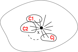
Figure 2: A node can be part of many primary clouds.

Free nodes and their choosing: The nodes of the primary clouds picked to form the secondary cloud are called non-free nodes. Thus free nodes are nodes that belong to only primary clouds. We note that a free node can belong to more than one primary cloud (see e.g., Figure 2). In the above construction of the secondary cloud, we choose one unique free node from each cloud, i.e., if there are $j$ clouds then we choose $j$ different nodes and associate each with one unique primary cloud (if a free node belongs to two or more primary clouds, we associate it with only one of them) such that each primary cloud has exactly one free node associated with it. (How this is implemented is deferred to Section 5.) We call the free node associated with a particular primary cloud as the bridge node that “connects” the primary cloud with the secondary cloud. Note that our construction implies that any (bridge) node of a primary cloud can belong to at most one secondary cloud.

What if there are no free nodes associated with a primary cloud, say $C$? Then we pick a free node (say $w$) from another cloud among the $j$ primary clouds (say $C^{\prime}$) and share the node with the cloud $C$. Sharing means adding $w$ to $C$ and forming a new $\kappa$-regular expander among the remaining nodes of $C$ (including $w$). Thus $w$ will be part of both $C$ and $C^{\prime}$ clouds. $w$ will be used as a free node associated with $C$ for the subsequent repair. Note that this might render $C^{\prime}$ devoid of free nodes. To compensate for this, $C^{\prime}$ gets a free node (if available) from some other cloud (among the $j$ primary clouds). Thus, in effect, every cloud will have its own free node associated with it, if there are at least $j$ free nodes (totally) among the $j$ clouds.

There is only one more possibility left to the discussed. If there are less than $j$ free nodes among all the $j$ clouds, then we combine all the $j$ primary clouds into a single primary cloud, i.e., we construct a $\kappa$-regular expander among all the nodes of the $j$ primary cloud (the previous edges belonging to the clouds are deleted). The edges of the new cloud will have a new (unique) color associated with it. Also all non-free nodes associated with the previous $j$ clouds become free again in the combined cloud. We note that combining many primary clouds into one primary cloud is a costly operation (involves a lot of restructuring). We amortize this costly operation over many cheaper operations. This is the main intuition behind constructing a secondary expander and free nodes; constructing a secondary expander is cheaper than combining many primary expanders and this is not possible only if there are no free nodes (which happens only once in a while).

Case 2.2: Some of the deleted edges are secondary edges. In other words, the deleted node, say $v$, will be a bridge (non-free) node. Let the deleted edges belong to the primary clouds $C_{1},C_{2},\dots,C_{j}$ and the secondary cloud $F$. (Our algorithm guarantees that a bridge node can belong to at most one secondary cloud.) We handle this deletion as follows. Let $v$ be the bridge node associated with the primary cloud $C_{i}$ (one among the $j$ clouds). Without loss of generality, let the secondary cloud connect a strict subset, i.e., $j^{\prime}<j$ primary clouds with possibly other (unaffected) primary clouds. This case is shown in Figure 3. As done in Case 2.1, we first fix all the $j$ primary clouds by constructing a new $\kappa$-regular expander among the remaining nodes. We then fix the secondary cloud by finding another free node, say $z$, from $C_{i}$, and reconstructing a new $\kappa$-regular secondary cloud expander on $z$ and other bridge nodes of other primary clouds of $F$. The edges retain the same color as their original. If there are no free nodes among all the primary clouds of $F$, then all primary clouds of $F$ are combined into one new primary cloud as explained in Case 2.1 above (edges of $F$ are deleted). The remaining $j-j^{\prime}$ primary clouds are then repaired as in case 2.1 by constructing a secondary cloud between them.

Figure 3: Case 2.2: Deleted node x part of secondary cloud F, and primary clouds

Algorithm 3.1 Xheal($\mathrm{G},\kappa$)

1:  if node $v$ inserted with incident edges then

2:     The inserted edges are colored black.

3:  if node $v$ is deleted then

4:     if all deleted edges are black then

5:        MakeCloud($BlackNbrs(v),primary,Clr_{new}$)

6:     else if deleted colored edges are all primary then

7:        Let $C_{1},\dots,C_{j}$ be primary clouds that lost an edge

8:        FixPrimary($[C_{1},\dots,C_{j}]$)

9:        MakeSecondary($[C_{1},\dots,C_{j}]\cup BlackNbrs(v)$)

10:     else

11:        Let $[C_{1},\dots,C_{j}]\leftarrow$ primary clouds of $v$; $F\leftarrow$ secondary cloud of $v$; $[U]\leftarrow$ $Clouds(F)\setminus[C_{1},\dots,C_{j}]$, $[C_{1},\dots,C_{j^{\prime}}]\leftarrow F\cap[C_{1},\dots,C_{j}]$

12:        FixPrimary($[C_{1},\dots,C_{j}]$)

13:        FixSecondary($F,v$)

14:        MakeSecondary($[C_{j^{\prime}+1},\dots,C_{j}]\cup BlackNbrs(v)$)

Algorithm 3.2 MakeCloud($[V],Type,Clr$)

1:  if $|V|\leq\kappa+1$ then

2:     Make clique among $[V]$

3:  else

4:     Make $\kappa$-reg expander among $[V]$ of edge $(Type,Clr)$

Algorithm 3.3 FixPrimary($[C]$)

1:  for each cloud $C_{i}\in[C]$  do

2:     MakeCloud($C_{i},primary,Color(C_{i})$)

Algorithm 3.4 MakeSecondary($[C]$)

1:  for each cloud $C_{i}\in[C]$  do

2:     if $FrNode_{i}$ = PickFreeNode($C_{i}$) == NULL then

3:        MakeCloud($Nodes([C]),primary,Clr_{new}$)

4:        Return

5:  MakeCloud($\bigcup FrNode_{i}\ \forall C_{i}\in[C]$, secondary,$Clr_{new}$)

Algorithm 3.5 FixSecondaryCloud($F,v$)

1:  if $v$ is a bridge node of $C_{i}$ in $F$ then

2:     if $FrNode_{i}$ = PickFreeNode($C_{i}$) == NULL then

3:        MakeCloud($Nodes(F),primary,Clr_{new}$)

4:     else

5:        MakeCloud($FrNode_{i}\cup BridgeNode(C_{j})\ \forall C_{i}\in[C]$, secondary, Color(F))

Algorithm 3.6 PickFreeNode()

1:  Let a Free node be a primary node without secondary duties

2:  if Free node in my cloud then

3:     Return Free node

4:  else

5:     Ask neighbor clouds; if a free node found, return node, else return NULL

4 Analysis of Xheal

The following is our main theorem on the guarantees that Xheal provides on the topological properties of the healed graph. The theorem assumes that Xheal is able to construct a $\kappa$-regular expander (deterministically) of expansion $\alpha>2$.

Theorem 2.

For graph $G_{t}$(present graph) and graph $G^{\prime}_{t}$ (of only original and inserted edges), at any time t, where a timestep is an insertion or deletion followed by healing:

1. For all $x\in G_{t}$, $degree_{G_{t}}(x)\leq\kappa.degree_{G^{\prime}_{t}}(y)$, for a fixed constant $\kappa>0$.

2. For any two nodes $u,v\in G_{t}$, $\delta_{G_{t}}(u,v)\leq\delta_{G^{\prime}_{t}}(u,v)O(\log n)$, where $\delta(u,v)$ is the shortest path between $u$ and $v$, and $n$ is the number of nodes in $G_{t}$.

3. $h(G_{t})\geq min(\alpha,h(G^{\prime}_{t}))$, for some fixed constant $\alpha\geq 1$.

4. $\lambda(G_{t})\geq min\left(\Omega\left(\frac{\lambda(G^{\prime}_{t})^{2}d_{min}(G^{\prime}_{t})}{(\kappa)^{2}(d_{max}(G^{\prime}_{t}))^{2}}\right),\Omega\left(\frac{1}{(\kappa d_{max}(G^{\prime}_{t}))^{2}}\right)\right)$, where $d_{min}(G^{\prime}_{t})$ and $d_{max}(G^{\prime}_{t})$ are the minimum and maximum degrees of $G^{\prime}_{t}$.

From the above theorem, we get an important corollary:

Corollary 1.

If $G^{\prime}_{t}$ is a (bounded degree) expander, then so is $G_{t}$. In other words, if the original graph and the inserted edges is an expander, then Xheal guarantees that the healed graph also is an expander.

4.1 Expansion, Degree and Stretch

Lemma 1.

Suppose at the first timestep (t=1), a deletion occurs. Then, after healing, $h(G_{1})\geq min(c,h(G^{\prime}_{1}))$, for a constant $c\geq 1$.

Proof.

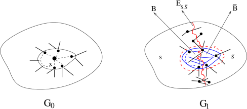
Figure 4: Healed graph after deletion of node $x$. The ball of $x$ and its neighbors gets replaced by a $\kappa$-regular expander of its neighbors — Case 1 of the Algorithm.

Observe that the initial graphs $G_{0}$ and $G^{\prime}_{0}$ are identical. Suppose that node $x$ is deleted at $t=1$. For ease of notation, refer to the graph $G_{0}$ as $G$ and the healed graph $G_{1}$ as $H$. Notice that $G^{\prime}_{1}$ is the same as $G_{0}$, since the graph $G^{\prime}_{t}$ does not change if the action at time $t$ is a deletion. Consider the induced subgraph formed by $x$ and its neighbors. Since all the deleted edges are black edges, Case 1 of the algorithm applies. Thus the healing algorithm will replace this subgraph by a new subgraph, a $\kappa$-regular expander over $x$’s ex-neighbors. Let us call this new subgraph $I$. Note that this corresponds to Case 1 of the Algorithm. We refer to Figure 4.

Consider a set $S(H)$ which defines the expansion in $H$ i.e. $|S(H)|\leq n/2$ (where $n$ is the number of nodes in $G$), and $S(H)$ has the minimum expansion over all the subsets of $H$. Call the cut induced by $S(H)$ as $E_{S,\bar{S}}(H)$ and its size as $|E|_{S,\bar{S}}(H)$. Also refer to the same set in $G$ (without $x$ if $S(H)$ included $x$) as $S(G)$, and the cut as $E_{S,\bar{S}}(G)$. The key idea of the proof is to directly bound the expansion of $H$, instead of looking at the change of expansion from of $G$. In particular, we have to handle the possibility that our self-healing algorithm may not add any new edges, because those edges may already be present. (Intuitively, this means that the prior expansion itself is good.)

We consider two cases depending on whether the healing may or may not have affected this cut.

1. $E_{S,\bar{S}}(H)\cap E(I)=\emptyset$:

   This implies that only the edges which were in $G$ are involved in the cut $E_{S,\bar{S}}(H)$. Since expansion is defined as the minimum over all cuts, $|\mathrm{E}|_{S,\bar{S}}(G)\geq h(G)|S(G)|$. Also, since $\mathrm{E}_{S,\bar{S}}(H)=\mathrm{E}_{S,\bar{S}}(G)$ and $S(H)\leq S(G)$, we have:

   $$h(H)=\frac{\mathrm{E}_{S,\bar{S}}(H)}{S(H)}\geq\frac{\mathrm{E}_{S,\bar{S}}(G)}{S(G)}\geq h(G).$$

2. $E_{S,\bar{S}}(H)\cap E(I)\neq\emptyset$: Notice that if there is any minimum expansion cut not intersecting $E(I)$, part 1 applies, and we are done.

   The healing algorithm tries to add enough new edges (if needed) into $I$ so that $I$ itself has an expansion of $\alpha>2$ (cf. Algorithm in Section 3). Note that it may not succeed if $|I|$ is too small. However, in that case, the algorithm makes $I$ a clique and achieves an expansion of $c$ where $c\geq 1$. Thus, we have the following cases:

   1. $I$ has an expansion of $\alpha>2$:
      Consider the nodes in $I$ which are part of $S(H)$ i.e., $B=S(H)\cap I$. We want to calculate $h(H)$. Since expansion is defined over sets of size not more than half of the size of the graph, we can do so in two ways:

      1. $B\leq I/2$: $S(H)$ expands at least as much as $h(G)$ except for the edges lost to $x$, and our algorithm ensures that $I$ has expansion of at least $\alpha>2$. Therefore, we have:

         $$h(H) = \frac{\mathrm{E}_{S,\bar{S}}(H)}{S(H)}$$

         $$\geq \frac{(|S(H)|-|B|).h(G)-|B|+|B|.\alpha}{|S(H)|}$$

         $$= \frac{(|S(H)|-|B|).h(G)+|B|.(\alpha-1)}{|S(H)|}$$

         In the numerator above, we have $(|S(H)|-|B|).h(G)$ which is a lower bound for the number of edges emanating from the set $S(H)$ (we minus $|B|$ from $|S(H)|$ to account for the edges that may be already present, note that Xheal does not add edges between two nodes if they are already present.) We subtract another $|B|$ or the edges lost to the deleted node and add $|B|\alpha$ edges due to the expansion gained.

         The following cases arise: If $h(G)\geq\alpha-1$, we have $h(H)\geq\frac{|S(H)|(\alpha-1)}{|S(H)|}\geq\alpha-1>1$. Otherwise, if $h(G)\leq\alpha-1$, we get: $h(H)\geq\frac{|S(H)|.h(G)}{|S(H)|}\geq h(G)$

      2. $\bar{B}\leq I/2$: By construction, nodes of $\bar{B}$ expand with expansion at least $\alpha$ in the subgraph $I$. Similar to above, we get, $h(H)\geq\frac{(|S(H)|-|\bar{B}|).h(G)+|\bar{B}|.(\alpha-1)}{|S(H)|}$. Thus, if $h(G)\geq\alpha-1$, then $h(H)\geq\alpha-1$, else $h(H)\geq h(G)$.

   2. $I$ has an expansion of $c<\alpha$:
      This happens in the case of the degree of $x$ being smaller than $k$. In this case, the expander $I$ is just a clique. Note that, even if degree of $x$ is 2, the expansion is 1. (When the degree of $x$ is 1, then the deleted node is just dropped, and it is easy to show that in this case, $h(H)\geq h(G)$.) The same analysis as the above applies, and we get $h(H)\geq min(c^{\prime},h(G))$, for some constant $c^{\prime}\geq 1$. Since $G$ is $G_{1}$ and $H$ is $G^{\prime}_{1}$, we get $h(G_{1})\geq min(c^{\prime},h(G^{\prime}_{1}))$.

∎

Corollary 2.

Given a graph $G$, and a subgraph $B$ of $G$, construct a new graph $H$ as follows: Delete the edges of $B$ and insert an expander of expansion $\alpha>2$ among the nodes of $B$. Then $h(H)\geq\min(c,h(G))$, where $c$ is a constant.

Lemma 2.

At end of any timestep t, $h(G_{t})\geq min(c^{\prime},h(G^{\prime}_{t}))$, where $c^{\prime}\geq 1$ is a fixed constant.

Proof.

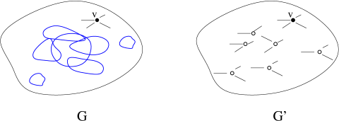
Figure 5: Graphs $G_{t}$ and $G^{\prime}_{t}$ after insertion of node $v$. Graph $G_{t}$ has some colored clouds. The nodes which have already been deleted are present in graph $G^{\prime}_{t}$ and are shown as unfilled nodes.

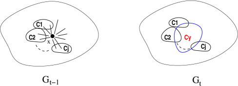
Figure 6: Healed graph after deletion of node $x$. The ’black’ neighbors of $x$ and some neighbors of $x$ from color clouds $C_{1},C_{2},\ldots C_{j}$ get connected by a $\kappa$-regular expander of color $C_{y}$.

First, consider the case when node $v$ is inserted at time $t$. Observe that the topologies of both the graphs $G_{t}$ and $G^{\prime}_{t}$ would be the same if all the insertions were to happen before the deletions. This is because an incoming node comes in with only black edges and at no step does the healing algorithm rely on the number of nodes present or uses edges for possible future nodes. Therefore, for our analysis, consider an order in which all the insertions happened before the first deletion, in particular think of node $v$ as being inserted at time $s$, and the first deletion happening at time $s+1$. Since the graphs $G_{i}$ and $G^{\prime}_{i}$ would look exactly the same for all $i$ before $s+1$, insertion of node $v$ changes both the graphs $G_{t}$ and $G^{\prime}_{t}$ in exactly the same way. Thus, if we can show that our lemma holds when a deletion happens (as we show below), we are done.

Next, we consider that a deletion occurs at timestep $t$. The proof will be by induction on $t$. Lemma 1 already shows the base case, where it is assumed wlog that the first deletion occurs at time $t=1$. Notice that before the first deletion, graphs $G$ and $G^{\prime}$ are identical and the proof is trivial.

As per the algorithm, we have two main cases to consider.

Case 1: This case occurs when the deleted edges are all black edges. This case is handled exactly as in the proof of Lemma 1.

Case 2.1 and Case 2.2: We analyze Case 2.1 below, the analysis of Case 2.2 is similar.

First, we give the proof assuming that each cloud has a free node associated with it.

Refer to figure 6. Let $G$ be the original graph and $H$ the healed graph. Let $x$ be the node deleted. The graph $G$ corresponds to the graph $G_{t-1}$. The graph $G^{\prime}_{t-1}$ is the same as the graph $G^{\prime}_{t}$ since the graph $G^{\prime}$ does not change on deletion. By the induction hypothesis, $h(G)=h(G_{t-1})\geq min(c,h(G^{\prime}_{t-1})=h(G^{\prime}_{t}))$. The graph $H$ corresponds to the healed graph $G_{t}$. Thus, if we show $h(H)\geq h(G)$, we are done.

In this case, let the deleted node $x$ belong to $j$ primary clouds $C_{1}$ to $C_{j}$. (We note that if $x$ has black neighbors, the algorithm treats them as singleton primary clouds.) First the primary clouds are restructured by constructing a new $k$-regular expander among the remaining nodes of the cloud (excluding the deleted node). Then, a free node from each color cloud is picked and are connected to form a $\kappa$-regular expander of color, say, $C_{x}$ — this is the secondary cloud.

The proof is a generalization of the argument of Lemma 1. Let $E_{S}((H)$ be a cut that defines the expansion in the graph $H$, and $S_{H}$ as defined before . Let us call this a minimum cut. If any minimum cut $E_{S}(H)$ passes through only the edges of $E(G)-(E(C_{1})\cup\dots\cup E(C_{j})\cup E(C_{x})$ (i.e., outside these clouds) then the expansion of $H$ cannot decrease and we are done. Thus, we will consider the cases when all minimum cuts pass through some edges of the above clouds.

Each of the colored balls maintains an expansion of at least $\alpha>2$. Let $B_{1},B_{2},\ldots B_{j}$, $B_{x}$, be the nodes of $S_{H}$ in the balls of color $C_{1},C_{2},\ldots C_{j}$, $C_{x}$ respectively. (We abuse notation so that each $C_{i}$ also denotes the subgraph defining the respective primary cloud.) In the following, for $1\leq i\leq j$, we define $A_{i}=B_{i}$ if $|B_{i}|\leq|C_{i}|/2$, otherwise, we define $A_{i}=\bar{B_{i}}=C_{i}-B_{i}$ if $|B_{i}|\geq|C_{i}|/2$. $A_{x}$ is similarly defined.

We have:

$$h(H) \geq \frac{(|S(H)|-\sum_{i=1}^{x}|A_{i}|)h(G)-\sum_{i=1}^{x}|A_{i}|+\sum_{i=1}^{x}|A_{i}|\alpha}{|S(H)|}$$

$$= \frac{(|S(H)|-\sum_{i=1}^{x}|A_{i}|)h(G)+(\sum_{i=1}^{x}|A_{i}|)(\alpha-1)}{|S(H)|}$$

If $h(G)\geq\alpha-1$, we have:

$$h(H) \geq\alpha-1>1$$

If $h(G)\leq\alpha-1$, we have:

$$h(H) \geq h(G)$$

Thus, $h(G_{t})=min(c^{\prime},h(G^{\prime}_{t}))$, for some $c^{\prime}=min(c,\alpha-1)$ and the induction hypothesis holds.

The above analysis assumes that each primary cloud had a free node for itself. Otherwise, as per the algorithm, free nodes from other clouds are shared. If there there a total of $j$ free nodes among all the $j$ clouds, then also the analysis proceeds as above. The only difference is that when a free node is shared between two clouds, its degree increases (by $k$). This can only increase the expansion, and hence the above analysis goes through. The other possibility is that there are less than $j$ free nodes. In this case, all the primary clouds are combined into one single expander cloud. Here also, the analysis is similar to above. ∎

Lemma 3.

For all $x\in G_{t}$, $degree_{G_{t}}(x)\leq O(\kappa.degree_{G^{\prime}_{t}}(x))$, for a fixed parameter $\kappa>0$.

Proof.

We bound the increase in degree of any node $x$ that belongs to both $G_{t}$ and $G^{\prime}_{t}$. Let the degree of $x$ in $G^{\prime}_{t}$ be $d^{\prime}(x)=degree_{G^{\prime}_{t}}(x)$. This will be black-degree of $x$ (as $G^{\prime}_{t}$ comprises solely of edges present in the original graph plus the inserted edges). There are three cases to consider and we bound the degree increase in each:

1. Whenever, a black edge gets deleted from this node, the self-healing algorithm, adds $\kappa$ colored edges in place of it, because a $\kappa$-regular expander is constructed which includes this node (this expander can be a primary or a secondary cloud). Thus $x$’s degree can increase by a factor of $\kappa$ at most because of deletion of black edges.

2. When $x$ loses a colored edge, then the algorithm restructures the expander cloud by constructing a new $\kappa$-regular expander. Again, this is true if the reconstruction is done on a primary or a secondary cloud. In this case, the degree of $x$ does not change.

3. Finally, we consider the effect of non-free nodes. $x$’s degree can increase if it is chosen as a bridge (non-free) node to connect a primary cloud (with which it is associated) to a secondary cloud. In this case, its degree will increase by $\kappa$, since it will become part of the secondary cloud expander. There is one more possibility that can contribute to increase of $x$’s degree by $\kappa$ more. If $x$ is chosen to be shared as a free node, i.e., it gets associated as a free node with another primary cloud than it originally belongs to, then its degree increases by $\kappa$ more, since it becomes part of another $\kappa$-regular expander. The shared node becomes a bridge node, i.e., a non-free node in that time step. Hence it cannot be shared henceforth.

From the above, we can bound the degree of $x$ in $G_{t}$, $d(x)=degree_{G_{t}}(x)$, as follows: $d(x)\leq\kappa d^{\prime}(x)+2\kappa.$ The lemma follows. ∎

Lemma 4.

For any two nodes $u,v\in G_{t}$,
$\delta_{G_{t}}(u,v)\leq\delta_{G^{\prime}_{t}}(u,v).O(\log n)$, where $\delta(u,v)$ is the shortest path between $u$ and $v$, and $n$ is the total number of nodes in $G_{t}$.

Proof.

We fix two nodes $u$ and $v$ and let the shortest distance between them in $G^{\prime}_{t}$ be $\ell$. Since this is on the graph $G^{\prime}_{t}$ (which comprises the original edges plus inserted edges), all the edges on this path will be black edges. Let this shortest path be denoted by $P=<u,u_{1},\dots,u_{\ell-1},v>$. We assume that $\ell>1$, because the path will just be the edge $(u,v)$ if $\ell=1$ in which case there is nothing to prove (the edge will also be present in $G_{t}$).

If all the intermediate nodes are present, then the result follows trivially. Otherwise, let $u^{\prime}_{1},u^{\prime}_{2},\dots,u^{\prime}_{i}$ ($i\leq\ell$) be the $i$ deleted nodes listed in the order of their deletion (i.e., $u^{\prime}_{1}$ was deleted before $u^{\prime}_{2}$ and so on).

We show that each node deletion can increase the distance between $u$ and $v$ by $O(\log n)$. Consider the deletion of node $u^{\prime}_{1}$. This will create a $k$-regular expander (primary or secondary, the latter case will arise if some incident edges of $u^{\prime}_{1}$ are colored) among the neighbors of $u^{\prime}_{1}$ in path $P$. Thus the distance between these neighbors of $u^{\prime}_{1}$ will increase by $O(\log(deg(u^{\prime}_{1}))=O(\log n)$. We distinguish two cases for subsequent deletions:

1. When the deleted node, say $u^{\prime}_{j}$, results in a primary cloud: In this case, the distance between the neighbors of $u^{\prime}_{j}$ will increase by at most $O(\log n)$, as above. Note that any subsequent deletion of nodes belonging to the primary cloud will still keep the same stretch, as there will always be connected via a $k$-regular expander.

2. When the deleted node, say $u^{\prime}_{j}$, results in a secondary cloud: In this case, there are two possibilities: (a) If the secondary cloud does not comprise primary clouds formed from previous deletions of nodes in the path $P$. In this case, the increase in distance is $O(\log n)$ as above; (b) If the secondary cloud comprises primary clouds formed from prior deletions of nodes in $P$, then the distance between $u$ and $v$ increases also by $O(\log n)$, as one has to traverse through the secondary cloud (connecting the primary clouds).

Thus, the overall distance between $u$ and $v$ increases by a factor of $O(\log n)$ in $G_{t}$ compared to the distance in $G^{\prime}_{t}$.

∎

4.2 Spectral Analysis

We derive bounds on the second smallest eigenvalue $\lambda$ which is closely related to properties such as mixing time, conductance etc. While it is directly difficult to derive bounds on $\lambda$, we use our bounds on edge expansion and the Cheeger’s inequality to do so.

We need the following simple inequality which relates the Cheeger constant $\phi(G)$ and the edge expansion $h(G)$ of a graph $G$ which follows from their respective definitions. We use $d_{max}(G)$ and $d_{min}(G)$ to denote the maximum and minimum node degrees in $G$.

$$\frac{h(G)}{d_{max}(G)}\leq\phi(G)\leq\frac{h(G)}{d_{min}(G)}.$$ (1)

Proof.

By Cheeger’s inequality and by inequality 1 we have,

$$\lambda(G_{t})\geq\frac{\phi(G_{t})^{2}}{2}\geq\frac{1}{2}\left(\frac{h(G_{t})}{d_{max}(G_{t})}\right)^{2}$$

By Lemma 2, we have, $h(G_{t})\geq min(c^{\prime},h(G^{\prime}_{t}))$, for some $c^{\prime}\geq 1$.

So we have two cases:

Case 1: $h(G_{t})\geq h(G^{\prime}_{t})$. By using the other half of Cheeger’s inequality, and inequality 1, and Lemma 3 we have:

$$\lambda(G_{t}) \geq \frac{1}{2}\left(\frac{h(G^{\prime}_{t})}{d_{max}(G_{t})}\right)^{2}$$

$$\geq \frac{1}{2}\left(\frac{\lambda(G^{\prime}_{t})d_{min}(G^{\prime}_{t})}{2d_{max}(G_{t})}\right)^{2}$$

$$\geq \frac{\lambda(G^{\prime}_{t})^{2}}{8(\kappa)^{2}}\frac{d_{min}(G^{\prime}_{t})}{(d_{max}(G^{\prime}_{t}))^{2}}$$

$$= \Omega\left(\lambda(G^{\prime}_{t})^{2}\frac{d_{min}(G^{\prime}_{t})}{(\kappa)^{2}(d_{max}(G^{\prime}_{t}))^{2}}\right).$$

Case 2: $h(G_{t})\geq 1$:

This directly gives:

$$\lambda(G_{t}) \geq \frac{1}{2}\left(\frac{1}{d_{max}(G_{t})}\right)^{2}$$

$$\geq \Omega\left(\frac{1}{(d_{max}(G_{t}))^{2}}\right)$$

$$\geq \Omega\left(\frac{1}{(\kappa d_{max}(G^{\prime}_{t}))^{2}}\right).$$

∎

5 Distributed Implementation of Xheal: Time and Message Complexity Analysis

We now discuss how to efficiently implement Xheal . A key task in Xheal involves the distributed construction and maintenance (under insertion and deletion) of a regular expander. We use a randomized construction of Law and Siu [20] that is described below. The expander graphs of [20] are formed by constructing a class of regular graphs called H-graphs. An H-graph is a $2d$-regular multigraph in which the set of edges is composed of $d$ Hamilton cycles. A random graph from this class can be constructed (cf. Theorem below) by picking $d$ Hamilton cycles independently and uniformly at random among all possible Hamilton cycles on the set of $z\geq 3$ vertices, and taking the union of these Hamilton cycles. This construction yields a random regular graph (henceforth called as a random H-graph) that that can be shown to be an expander with high probability (cf. Theorem 4). The construction can be accomplished incrementally as follows.

Let the neighbors of a node $u$ be labeled as
$nbr(u)_{-1},nbr(u)_{1},nbr(u)_{-2},...,nbr(u)_{-d},nbr(u)_{d}$. For each $i$, $nbr(u)_{-i}$ and $nbr(u)_{i}$ denote a node’s predecessor and successor on the $i$th Hamilton cycle (which will be referred to as the level-$i$ cycle). We start with 3 nodes, because there is only one possible H-graph of size 3.

1.INSERT(u): A new node $u$ will be inserted into cycle $i$ between node $v_{i}$ and node $nbr(v_{i})_{i}$ for randomly chosen $v_{i}$, for $i=1,\dots,d$.

2. DELETE(u): An existing node $u$ gets deleted by simply removing it and connecting $nbr(u)_{i}$ and $nbr(u)_{-i}$, for $i=1,\dots,d$.

Law and Siu prove the following theorem (modified here for our purposes) that is used in Xheal :

Theorem 3 ([20]).

Let $H_{0},H_{1},H_{2},\dots$ be a sequence of $H$-graphs, each of size at least 3. Let $H_{0}$ be a random $H$-graph of size $n$ and let $H_{i+1}$ be formed from $H_{i}$ by either INSERT or DELETE operation as above. Then $H_{i}$ is a random $H$-graph for all $i\geq 0$.

Theorem 4 ([9, 20]).

A random $n$-node $2d$-regular $H$-graph is an expander (with edge expansion $\Omega(d)$) with probability at least $1-O(n^{-p})$ where $p$ depends on $d$.

Note that in the above theorem, the probability guarantee can be made as close to 1 as possible, by making $d$ large enough. Also it is known that $\lambda$, the second smallest eigenvalue, for these random graphs is close to the best possible [9]. Another point to note that although the above construction can yield a multigraph, it can be shown that similar high probabilistic guarantees hold in case we make the multi-edges simple, by making $d$ large enough. Hence we will assume that the constructed expander graphs are simple.

We next show how Xheal algorithm is implemented and analyze the time and message complexity per node deletion. We note that insertion of a node by adversary involves almost no work from Xheal . The adversary simply inserts a node and its incident edges (to existing nodes). Xheal simply colors these inserted edges as black. Hence we focus on the steps taken by Xheal under deletion of a node by the adversary. First we state the following lower bound on the amortized message complexity for deletions which is easy to see in our model (cf. Section 2). Our algorithm’s complexity will be within a logarithmic factor of this bound.

Lemma 5.

In the worst case, any healing algorithm needs $\Theta(deg(v))$ messages to repair upon deletion of a node $v$, where $deg(v)$ is the degree of $v$ in $G^{\prime}_{t}$ (i.e., the black-degree of $v$). Furthermore, if we there are $p$ deletions, $v_{1},v_{2},\dots,v_{p}$, then the amortized cost is $A(p)=(1/p)\sum_{i=1}^{p}\Theta(deg(v_{i}))$ which is the best possible.

Theorem 5.

Xheal can be implemented to run in $O(\log n)$ rounds (per deletion). The amortized message complexity over $p$ deletions is $O(\kappa\log nA(p))$ on average where $n$ is the number of nodes in the network (at this timestep), $\kappa$ is the degree of the expander used in the construction, and $A(p)$ is defined as in Lemma 5.

Proof.

(Sketch) We first note that the healing operations will be initiated by the neighbors of the deleted node. We also note that primary and secondary expander clouds can be identified by the color of their edges (cf. Algorithm in Section3.)

Case 1: This involves constructing a (primary) expander cloud among the neighboring nodes $N(v)$ of the deleted node $v$. Note that $|N(v)|=deg(v)$, where $deg(v)$ is the black-degree of $v$. Since each node knows neighbor of neighbor’s (NoN) addresses, it is akin to working on a complete graph over $N(v)$. We first elect a leader among $N(v)$: a random node (which is useful later) among $N(v)$ is chosen as a leader. This can be done, for example, by using the Nearest Neighbor Tree (NNT) algorithm of [khan-tcs]. This takes $O(\log|N(v)|)$ time and $O(|N(v)|\log|N(v)|)$ messages. The leader then (locally) constructs a random $\kappa$-regular $H$-graph over $N(v)$ and informs each node in $N(v)$ (directly, since its address is known) of their respective edges. The total messages needed to inform the nodes is $O(\kappa|N(v)|)$, since that is the total number of edges. A neighbor of the leader in the expander graph is also elected as a vice-leader. This can be implemented in $O(1)$ time. Hence, overall this case takes $O(\log|N(v)|)=O(\log deg(v))=O(\log n)$ time and $O(\kappa deg(v)\log deg(v))$ messages.

In particular, the following invariants will be maintained with respect to every expander (primary or secondary) cloud: (a) Every node in the cloud will have a leader (randomly chosen among the nodes) associated with it ; (b) every node in the cloud knows the address of the leader and can communicate with it directly (in constant time); and (c) the leader knows the addresses of all other nodes in the cloud; (d) one neighbor of the leader in the cloud will be designated vice-leader which will know everything the leader knows and will take action in case the leader is deleted. Note that this invariant is maintained in Case 1. We will show that it is also maintained in Case 2 below.

Case 2 (Cases 2.1 and 2.2 of Xheal): We have to implement three main operations in these cases. They are:
(a) Reconstructing an expander cloud (primary or secondary) on deletion of a node $v$: Let $C$ be the primary (or secondary) cloud that loses $v$. The node is removed according to the DELETE operation of $H$-graph. This takes $O(1)$ time and $O(\kappa)$ messages. If $v$ belongs to $j$ primary clouds then the time is still $O(1)$ while the total message complexity is $O(j\kappa)$. For $v$ to belong to $j$ primary clouds its black degree should be at least $j$. Also $v$ can belong to at most one secondary cloud. Hence the cost is at most $O(\kappa)$ times the black degree as needed. If the deleted node happens to be the leader of the (primary) cloud then a new random leader is chosen (by the vice-leader) and inform the rest of the nodes — this will take $O(|C|)$ messages and $O(1)$ time, where $|C|$ is the number of nodes in the cloud. Since the adversary does not know the random choices made by the algorithm, the probability that it deletes a leader in a step is $1/|C|$ and thus the expected message complexity is $O((1/|C|)|C|=O(1)$. (Note that a new vice-leader, a neighbor of the new leader will be chosen if necessary.)

(b) Forming and fixing primary and secondary expander clouds (if there are enough free nodes): Let the deleted node belong to primary clouds $C_{1},\dots,C_{j}$ and possibly a secondary cloud $F$ that connects a subset of these $j$ clouds (and possibly other unaffected primary clouds). First, each of the clouds are reconstructed as in (a) above. This operation arises only if we have at least $j$ free nodes, i.e., nodes that are not associated with any secondary cloud. We now mention how free nodes are found. To check if there are enough free nodes among the $j$ clouds, we check the respective leaders. The leader always maintain a list of all free nodes in its cloud. Thus if a node becomes non-free during a repair it informs the leader (in constant time) which removes it from the list. Thus the neighbors of the deleted node can request the leaders of their respective clouds to find free nodes. Hence finding free nodes takes time $O(1)$ and needs $O(j)$ messages. The free nodes are then inserted to form the secondary cloud. We distinguish two situations with respect to formation of a secondary cloud: (i) The secondary cloud is formed for the first time (i.e., a new secondary cloud among the primary clouds). In this case, a leader of one of the associated primary cloud is elected to construct the secondary expander. This leader then gets the free nodes from the respective primary clouds, locally constructs a $\kappa$-regular expander and informs it to the respective free nodes of each primary cloud. This is similar to the construction of a primary cloud as in (a). The time and message complexity is also bounded as in (a).

(ii)The secondary cloud is already present, merely, a new free node is added. In this case, the new node is inserted to the secondary cloud by using the INSERT operation of $H$-graph. This takes $O(1)$ time and $O(1)$ messages, since INSERT can be implemented by querying the leader.

(c) Combining many primary expander clouds into one primary expander cloud (if there are not enough free nodes): This is a costly operation which we seek to amortize over many deletions. First, we compute the cost of combining clouds. Let $C_{1},\dots,C_{j}$ are the clouds that need to be combined into one cloud $C$. This is done by first electing a leader over all the nodes in the clouds $C_{1},\dots,C_{j}$. Note that the distance between any two nodes among these clouds is $O(\log n)$, since all the clouds had a common node (the deleted node) and each cloud is an expander (also note that the neighbors of the deleted nodes maintain connectivity during the leader election and subsequent repair process). A BFS tree is then constructed subsequently over the nodes of the $j$ clouds with the leader as the root. The leader then collects all the addresses of all the nodes in the clouds (via the BFS tree) and locally constructs a $H$-graph and broadcasts it to all the other nodes in the cloud. The leader’s address is also informed to all the other nodes in the cloud. Thus the invariant specified in Case 1 is maintained. The total time needed is $O(\log n)$ time and the total number of messages needed is $O(\kappa\sum_{i=1}^{j}|C_{i}|)\log n$, since each node (other than the leader) sends $O(1)$ number of messages over $O(\log n)$ hops, and the leader sends $O(\sum_{i=1}^{j}|C_{i}|)\log n$. However, note that the costly operation of combining is triggered by having less than $j$ free nodes. This implies that there must been at least $\Omega(\sum_{i=1}^{j}|C_{i}|)$ prior deletions that had enough free nodes and hence involved no combining. Thus, we can amortize the total cost of the combining cost over these “cheaper” prior deletions. Hence the amortized cost is

$$\frac{O(\kappa\sum_{i=1}^{j}|C_{i}|)\log n}{\Omega(\sum_{i=1}^{j}|C_{i}|)}=O(\kappa\log n).$$

Finally, we say how the probabilistic guarantee on the $H$-graph can be maintained. The implementation above uses a $\kappa$-regular random $H$-graph in the construction of an expander cloud. By theorem 4, $\kappa$ can be chosen large enough to guarantee the probabilistic requirement needed. For example, choosing $\kappa=\Theta(\log n)$, then high probability (with respect to the size of the network) is guaranteed (this assumes that nodes know an upper bound on the size of the network). Furthermore, if there are $f$ deletions, by union bound, the probability that it is not an expander increases by up to a factor of $f$. To address this, we reconstruct the $H$-graph after any cloud has lost half of its nodes; note that the cost of this reconstruction can be amortized over the deletions to obtain the same bounds as claimed. ∎

6 Conclusion

We have presented an efficient, distributed algorithm that withstands repeated adversarial node insertions and deletions by adding a small number of new edges after each deletion. It maintains key global invariants of the network while doing only localized changes and using only local information. The global invariants it maintains are as follows. Firstly, assuming the initial network was connected, the network stays connected. Secondly, the (edge) expansion of the network is at least as good as the expansion would have been without any adversarial deletion, or is at least a constant. Thirdly, the distance between any pair of nodes never increases by more than a $O(\log n)$ multiplicative factor than what the distance would be without the adversarial deletions. Lastly, the above global invariants are achieved while not allowing the degree of any node to increase by more than a small multiplicative factor.

The work can be improved in several ways in similar models. Can we improve the present algorithm to allow smaller messages and lower congestion? Can we efficiently find new routes to replace the routes damaged by the deletions? Can we design self-healing algorithms that are also load balanced? Can we reach a theoretical characterization of what network properties are amenable to self-healing, especially, global properties which can be maintained by local changes? What about combinations of desired network invariants? We can also extend the work to different models and domains. We can look at designing algorithms for less flexible networks such as sensor networks, explore healing with non-local edges. We can also look beyond graphs to rewiring and self-healing circuits where it is gates that fail.

References

- [1] D. Andersen, H. Balakrishnan, F. Kaashoek, and R. Morris. Resilient overlay networks. SIGOPS Oper. Syst. Rev., 35(5):131–145, 2001.
- [2] V. Arak. What happened on August 16, August 2007. http://heartbeat.skype.com/2007/08/what-happened-on-august-16.html.
- [3] B. Awerbuch, B. Patt-Shamir, D. Peleg, and M. Saks. Adapting to asynchronous dynamic networks (extended abstract). In STOC ’92: Proceedings of the twenty-fourth annual ACM symposium on Theory of computing, pages 557–570, New York, NY, USA, 1992. ACM.
- [4] I. Boman, J. Saia, C. T. Abdallah, and E. Schamiloglu. Brief announcement: Self-healing algorithms for reconfigurable networks. In Symposium on Stabilization, Safety, and Security of Distributed Systems(SSS), 2006.
- [5] F. Chung. Spectral Graph Theory. American Mathematical Society, 1997.
- [6] S. Dolev and N. Tzachar. Spanders: distributed spanning expanders. In SAC, pages 1309–1314, 2010.
- [7] R. D. Doverspike and B. Wilson. Comparison of capacity efficiency of dcs network restoration routing techniques. J. Network Syst. Manage., 2(2), 1994.
- [8] K. Fisher. Skype talks of ”perfect storm” that caused outage, clarifies blame, August 2007. http://arstechnica.com/news.ars/post/20070821-skype-talks-of-perfect-storm.html.
- [9] J. Friedman. On the second eigenvalue and random walks in random d-regular graphs. Combinatorica, 11:331 362, 1991.
- [10] T. Frisanco. Optimal spare capacity design for various protection switching methods in ATM networks. In Communications, 1997. ICC 97 Montreal, ’Towards the Knowledge Millennium’. 1997 IEEE International Conference on, volume 1, pages 293–298, 1997.
- [11] C. Gkantsidis, M. Mihail, and A. Saberi. Random walks in peer-to-peer networks: Algorithms and evaluation. Performance Evaluation, 63(3):241–263, 2006.
- [12] S. Goel, S. Belardo, and L. Iwan. A resilient network that can operate under duress: To support communication between government agencies during crisis situations. Proceedings of the 37th Hawaii International Conference on System Sciences, 0-7695-2056-1/04:1–11, 2004.
- [13] Y. Hayashi and T. Miyazaki. Emergent rewirings for cascades on correlated networks. cond-mat/0503615, 2005.
- [14] T. Hayes, N. Rustagi, J. Saia, and A. Trehan. The forgiving tree: a self-healing distributed data structure. In PODC ’08: Proceedings of the twenty-seventh ACM symposium on Principles of distributed computing, pages 203–212, New York, NY, USA, 2008. ACM.
- [15] T. P. Hayes, J. Saia, and A. Trehan. The forgiving graph: a distributed data structure for low stretch under adversarial attack. In PODC ’09: Proceedings of the 28th ACM symposium on Principles of distributed computing, pages 121–130, New York, NY, USA, 2009. ACM.
- [16] K. C. Hillel and H. Shachnai. Partial information spreading with application to distributed maximum coverage. In PODC ’10: Proceedings of the 28th ACM symposium on Principles of distributed computing, New York, NY, USA, 2010. ACM.
- [17] P. Holme and B. J. Kim. Vertex overload breakdown in evolving networks. Physical Review E, 65:066109, 2002.
- [18] S. Hoory, N. Linial, and A. Wigderson. Expander graphs and their applications. Bulletin of the American Mathematical Society, 43(04):439–562, August 2006.
- [19] R. R. Iraschko, M. H. MacGregor, and W. D. Grover. Optimal capacity placement for path restoration in STM or ATM mesh-survivable networks. IEEE/ACM Trans. Netw., 6(3):325–336, 1998.
- [20] C. Law and K. Y. Siu. Distributed construction of random expander networks. In INFOCOM 2003. Twenty-Second Annual Joint Conference of the IEEE Computer and Communications Societies. IEEE, volume 3, pages 2133–2143 vol.3, 2003.
- [21] O. Malik. Does Skype Outage Expose P2P s Limitations?, August 2007. http://gigaom.com/2007/08/16/skype-outage.
- [22] M. Medard, S. G. Finn, and R. A. Barry. Redundant trees for preplanned recovery in arbitrary vertex-redundant or edge-redundant graphs. IEEE/ACM Transactions on Networking, 7(5):641–652, 1999.
- [23] M. Moore. Skype’s outage not a hang-up for user base, August 2007. http://www.usatoday.com/tech/wireless/phones/2007-08-24-skype-outage-effects-N.htm.
- [24] A. E. Motter. Cascade control and defense in complex networks. Physical Review Letters, 93:098701, 2004.
- [25] A. E. Motter and Y.-C. Lai. Cascade-based attacks on complex networks. Physical Review E, 66:065102, 2002.
- [26] K. Murakami and H. S. Kim. Comparative study on restoration schemes of survivable ATM networks. In INFOCOM, pages 345–352, 1997.
- [27] D. Peleg. Distributed Computing: A Locality Sensitive Approach. SIAM, 2000.
- [28] B. Ray. Skype hangs up on users, August 2007. http://www.theregister.co.uk/2007/08/16/skype_down/.
- [29] J. Saia and A. Trehan. Picking up the pieces: Self-healing in reconfigurable networks. In IPDPS. 22nd IEEE International Symposium on Parallel and Distributed Processing., pages 1–12. IEEE, April 2008.
- [30] B. Stone. Skype: Microsoft Update Took Us Down, August 2007. http://bits.blogs.nytimes.com/2007/08/20/skype-microsoft-update-took-us-down.
- [31] A. Trehan. Algorithms for self-healing networks. Dissertation, University of New Mexico, 2010.
- [32] B. van Caenegem, N. Wauters, and P. Demeester. Spare capacity assignment for different restoration strategies in mesh survivable networks. In Communications, 1997. ICC 97 Montreal, ’Towards the Knowledge Millennium’. 1997 IEEE International Conference on, volume 1, pages 288–292, 1997.
- [33] Y. Xiong and L. G. Mason. Restoration strategies and spare capacity requirements in self-healing ATM networks. IEEE/ACM Trans. Netw., 7(1):98–110, 1999.