Soft-Decision-Driven Channel Estimation
for Pipelined Turbo Receivers

Abstract

We consider channel estimation specific to turbo equalization for multiple-input multiple-output (MIMO) wireless communication. We develop a soft-decision-driven sequential algorithm geared to the pipelined turbo equalizer architecture operating on orthogonal frequency division multiplexing (OFDM) symbols. One interesting feature of the pipelined turbo equalizer is that multiple soft-decisions become available at various processing stages. A tricky issue is that these multiple decisions from different pipeline stages have varying levels of reliability. This paper establishes an effective strategy for the channel estimator to track the target channel, while dealing with observation sets with different qualities. The resulting algorithm is basically a linear sequential estimation algorithm and, as such, is Kalman-based in nature. The main difference here, however, is that the proposed algorithm employs puncturing on observation samples to effectively deal with the inherent correlation among the multiple demapper/decoder module outputs that cannot easily be removed by the traditional innovations approach. The proposed algorithm continuously monitors the quality of the feedback decisions and incorporates it in the channel estimation process. The proposed channel estimation scheme shows clear performance advantages relative to existing channel estimation techniques.
Index Terms—channel estimation, MIMO-OFDM, turbo equalization, sequential estimator

I Introduction

Combining the multiple-input multiple-output (MIMO) antenna method with orthogonal frequency division multiplexing (OFDM) and spatial multiplexing is a well-established wireless communication technique. Bit-interleaved coded modulation (BICM) [1] used in conjunction with MIMO-OFDM and spatial multiplexing (SM) is particularly effective in exploring both spatial diversity and frequency selectivity without significant design efforts on specialized codes [2, 3]. Turbo equalization [4], also known as iterative detection and decoding (IDD) in wireless applications [6], is well-suited for BICM-MIMO-OFDM for high data rate transmission with impressive performance potentials [5, 6].

A critical issue in realizing the full performance potential of a MIMO-OFDM system is significant performance degradation due to imperfect channel state information (CSI). The detrimental impact of imperfect CSI on MIMO detection is well known (see, for example, [7, 8]) and continues to be a great challenge in wireless communication system design. Previous works have identified desirable training patterns or pilot tones for estimating channel responses for MIMO systems [9, 10, 11, 12, 13]. However, with these methods the achievable data rate is inevitably reduced, especially when the number of channel parameters to be estimated increases (e.g., caused by an increased number of antennas).

Decision-directed (DD) channel estimation algorithms can be applied to the turbo receivers to improve channel estimation accuracy [17, 15, 14, 16]. However, inaccurate feedback decisions degrade the estimator performance [18]. Maximum-a-posteriori (MAP)-based DD algorithms discussed in [14, 15] can improve the estimation accuracy, but they require additional information like the channel probability density function. The DD channel estimation algorithm jointly working with IDD has been actively researched [20, 19, 21, 22, 23]. Among the existing research works, several papers have been devoted to iterative expectation-maximization (EM) channel estimation algorithms using extrinsic or a posteriori information fed back from the outer decoder [20, 19, 21]. Although the traditional EM-based estimation algorithms typically show outstanding performance, the heavy computation complexity and the iteration latency can be problematic for many practical applications. While an approximation scheme as discussed in [20] can reduce complexity, the performances of these approaches suffer from performance degradation as the number of antennas increases [19]. Also, the EM estimation algorithms need to be aided by pilot-based EM algorithms to guarantee a good performance[20, 21].

As an alternative approach to iterative EM channel estimation, Kalman-based channel estimators have been discussed that are effective against error propagation [22, 23]. The authors of [22, 23] have introduced a soft-input channel estimator that adaptively updates the channel estimates depending on feedback decision quality. The soft-input channel estimator of [22] evaluates the feedback decision quality by tracking the noise variance that includes the potential soft-decision error impact in its effort to improve the update process for the Kalman filter.

In the present work, we develop a Kalman-based channel estimator for MIMO-OFDM based on a specific pipelined turbo equalizer receiver architecture. Before setting up the Kalman estimator, a novel method for reducing decision error correlation is introduced. The proposed method constructs a refined innovation sequence by irregularly puncturing certain soft decisions that are deemed to be correlated with the previous decisions. The resulting algorithm is basically a linear sequential estimation algorithm and, as such, is Kalman-based in nature. We also weigh the estimated channel responses in the detection process according to the quality of the estimation.

A critical issue in turbo receiver design is long processing latency due to inherent iterative processing of information. Pipelined architecture reduces the latency and improves processing throughput in turbo receivers and thus is the prevailing choice of the implementation architecture [24, 25]. One interesting feature of the pipelined turbo equalizer is that multiple sets of soft-decisions become available at various processing stages. A tricky issue is that these multiple decisions from different pipeline stages have varying levels of reliability. Therefore, an adequate optimization strategy is required for the estimator to track the target channel while dealing with observation sets with different qualities. An optimum channel estimator is derived based on this principle for the pipelined turbo receiver.

In demonstrating the viability of the proposed schemes, a SM-MIMO-OFDM system is constructed to comply with the IEEE 802.11n high speed WLAN standard [26]. Section II discusses the channel and system model, and briefly touches upon the high-throughput pipelined IDD architecture. Section III discusses the method to set up an improved innovation sequence via puncturing. Next, the proposed soft-DD Kalman-based channel estimation methods are presented in section III. Mean squared error (MSE) analysis is provided in Section IV that validates the performance merits of the proposed schemes. In Section V, the convergence behavior is investigated via the extrinsic information transfer (EXIT) charts [28], and packet error rate (PER) simulation results are presented for performance evaluation. Finally conclusions are drawn in Section VI.

II Channel and System Model

We assume a SM-MIMO-OFDM transmitter where a data bit sequence is encoded by a convolutional channel encoder, and the encoded bit stream is divided into $N_{t}$ spatial streams by a serial-to-parallel demultiplexer. Each spatial stream is interleaved separately, and the interleaved streams are modulated using an $M$-ary quadrature amplitude modulation ($M$-QAM) symbol set $\mathcal{A}$ based on the Gray mapping. Since $Q$ binary bits form an $M$-QAM symbol, a binary vector ${\bf{b}}=[b_{0},b_{1},\cdots,b_{QN_{t}-1}]^{T}$ is mapped to a transmitted symbol vector $\mathbf{s}=\left[s_{1},s_{2},\cdots,s_{N_{t}}\right]^{T}$ (with $s_{i}\in\mathcal{A}$), taken from the set $\mathcal{A}^{Nt}$, a Cartesian product of $M$-QAM constellations. The $M$-QAM symbol sequence in each spatial stream is transmitted by an OFDM transmitter utilizing a fixed number of frequency subcarriers. For a particular subcarrier for the $n^{th}$ OFDM symbol, the received signal at the discrete Fourier transform (DFT) output can be written as

$$\mathbf{z}_{n}=\mathbf{H}\mathbf{s}_{n}+\mathbf{n}_{n}\ ,$$ (1)

where $\mathbf{z}_{n}=\left[z_{1}(n),z_{2}(n),\cdots,z_{N_{r}}(n)\right]^{T}$ is the received signal vector observed at the $N_{r}$ receive antennas, and $\mathbf{H}$ is the channel response matrix associated with all wireless links connecting $N_{t}$ transmit antennas with $N_{r}$ receive antennas antennas, and $\mathbf{n}_{n}$ is a vector of uncorrelated, zero-mean additive white Gaussian noise (AWGN) samples of equal variance set to ${\mathcal{N}}_{o}$.

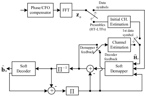
flushleft

Figure 1: Block diagram of the turbo receiver and the soft-decision-directed channel estimator

The IDD technique of [5] that performs turbo equalization for MIMO systems is assumed at the receiver. The extrinsic information on the coded-bit stream is exchanged in the form of log-likelihood ratio (LLR) between the soft-input soft-output (SISO) decoder and the SISO demapper as shown in Fig. 1. The demapper takes advantage of the reliable soft-symbol information made available by the outer SISO decoder. A soft-output Viterbi algorithm (SOVA) is used for the SISO decoder implementation [29]. Each data packet transmitted typically contains many OFDM symbols, and they are processed sequentially by the demapper and the decoder as they arrive at the receiver. The feedback decisions used for channel estimation must be interleaved coded-bit decisions. The extrinsic information from the demapper are rearranged accordingly and made available to the channel estimation block.

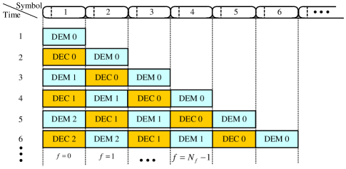
Figure 2: OFDM-symbol processing procedure in the pipelined IDD

The pipelined architecture is adopted to reduce the iteration latency  [24, 25]. Fig. 2 illustrates OFDM symbols processed in the pipelined IDD, and Fig. 3 shows the structure of the pipelined IDD receiver and its interface with the channel estimator. Multiple demapper-decoder pairs process multiple OFDM symbols at different iteration stages. Let $N_{itr}$ denote the number of the IDD iterations required to achieve satisfactory error rate performance. The $N_{itr}$-stage pipelined IDD receiver is equipped with $N_{itr}$ demappers and $N_{itr}$ decoders that are serially connected as in Fig. 3. The decoder forwards its extrinsic information output to the demapper in the next iteration stage. Simultaneously, the demapper and the decoder in the previous iteration stage start to process a new OFDM symbol. The pipelined IDD operation is functionally equivalent to the original IDD scheme [24].

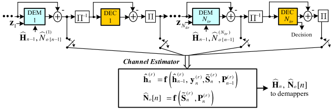
Figure 3: Block diagram of the proposed optimum channel estimation algorithm geared to the pipelined IDD

The extrinsic LLRs released from the pipelined demappers and decoders are utilized for the channel estimation. Let $N_{sym}$ denote the number of total OFDM symbols in a packet and $N_{f}$ the number of the feedback symbols available for channel estimation. Note, however, that not all $N_{f}$ symbols are used for the estimation. If the receiver requires $N_{itr}$ IDD iterations, then a maximum of $2N_{itr}$ OFDM symbols are processed in the pipelined IDD receiver as illustrated in Fig. 3. Because the LLR outputs from the initial demapper and decoder have low reliability, they are not used for the channel estimation. Let index $n$ indicate the time. In this pipelined IDD setup, when $2\leq n\leq 2N_{itr}$, the channel estimator can get ($n-2$) feedback decisions (i.e. $N_{f}=n-2$). When the number of the processed symbols increases to $2N_{itr}$ ($2N_{itr}\leq n\leq N_{sym}$), $N_{f}$ is equal to $2N_{itr}-2$. After all the OFDM symbols in the packet have arrived at the receiver front-end, it will take sometime until all symbols will clear out of the pipeline. For $n\geq N_{sym}$, $N_{f}$ is equal to $N_{sym}+2N_{itr}-n$.

III Sequential and Soft-Decision-Directed Channel Estimation

III-A Derivation of the Kalman-Based Sequential Channel Estimation Algorithm

The sequential form of the estimator is useful in improving the quality of the channel estimate as the observed symbols arrive in a sequential fashion, as OFDM symbols do in the system of our interest. It is assumed that the channel is quasi-static over $N_{f}$ OFDM symbol periods. For the pipelined IDD receiver at hand, the observation equation is set up at the $r^{th}$ receiver (RX) antenna as

$$\mathbf{z}^{(r)}_{n}=\mathbf{S}_{n}\mathbf{h}^{(r)}+\mathbf{n}^{(r)}_{n},\$$ (2)

where $\mathbf{z}_{n}^{(r)}$ is the ${N_{f}\times 1}$ received signal vector, $\mathbf{S}_{n}$ is a ${N_{f}\times N_{t}}$ matrix, $\mathbf{h}^{(r)}$ is a ${N_{t}\times 1}$ vector that is a multi-input-single-output (MISO) channel vector specific to the ${r^{th}}$ RX antenna. The goal is to do a sequential estimation of $\mathbf{h}^{(r)}$ as $n$ progresses. The estimation process is done in parallel to obtain channel estimates for all ${N_{r}}$ RX antennas. With an understanding that we focus on a specific RX antenna, the RX antenna index $r$ is dropped to reduce notation cluttering.

A mean symbol decision $\tilde{s}$ is defined as the average of the constellation symbols according $\tilde{s}=\tiny{\sum\nolimits_{\tiny{s_{i}\in{\mathcal{A}}}}{s_{i}P(s_{i})}}$, where $P(s_{i})$ is the “extrinsic probability” obtained from a direct conversion of the available extrinsic LLR.

III-A1 Innovation Sequence Setup

The pipeline architecture can be viewed as a buffer large enough to accommodate $N_{f}$ OFDM symbols, but we take into account in our channel estimator design the different levels of reliability for the soft decisions coming out of the demapper or decoder modules at different iteration stages. First, defining the soft decision error $\mathbf{E}\buildrel\Delta\over{=}\mathbf{S}-\widetilde{\mathbf{S}}$, (2) can be rewritten as

$$\mathbf{z}_{n}=\{\widetilde{\mathbf{S}}_{n}+\mathbf{E}_{n}\}{\bf{h}}+\mathbf{n}_{n}.$$ (3)

Note that this type of soft decision representation has been used previously  [22]. We emphasize, however, that unlike in [22], our derivation of a linear sequential estimator is based on the attempt to explicitly generate the innovation sequence. As will be clear in the sequel, this approach has led us to a realization that the standard steps taken to generate the innovations do not work in our set up; this in turn allowed us to devise corrective measures. Let us first see if we can find $\mathbf{x}_{n}$, the innovations of $\mathbf{z}_{n}$ (i.e., the whitened sequence that is a causal, as well as a casually invertible, linear transformation of $\mathbf{z}_{n}$). We write:

$$\mathbf{x}_{n} \buildrel\Delta\over{=} \mathbf{z}_{n}-\widetilde{\mathbf{S}}_{n}\hat{\mathbf{h}}_{n-1}$$ (4)

$$= \widetilde{\bf{S}}_{n}({\bf{h}}-\hat{\bf{h}}_{n-1})+{\bf{E}}_{n}{\bf{h}}+{\bf{n}}_{n}.$$ (5)

Ideally, the vector sequence $\mathbf{x}_{n}$ would represent an innovation sequence in the sense that any given component of the vector ${\bf{x}}_{n-k}$ is orthogonal to any component of ${\bf{x}}_{n}$ as long as $k\neq 0$. In this scenario we would have

$$E\left[{x_{n-k}[i]x_{n}^{*}[j]}\right]=E\left[{{\bf{e}}_{n-k}[i]\widehat{\bf{h}}_{n-k-1}{\bf{h}}^{H}{\bf{e}}_{n}^{H}[j]}\right]+\mathcal{N}_{o}$$

$$=\left\{{\begin{array}[]{*{20}c}{\sum\nolimits_{t=1}^{N_{t}}{\hat{\rho}_{n-1}^{(t)}}\sigma_{s}^{2}[t,i]}+\mathcal{N}_{o}&{{\rm{when}}\,\,k=0\,\,{\rm{and}}\,\,i=j}\\ \epsilon(\approx 0)&{{\rm{otherwise}}},\\ \end{array}}\right.$$ (8)

where ${\bf{e}}_{n}[i]$ indicates the $i^{th}$ row vector ${\bf{E}}_{n}$, ${\hat{\rho}_{n-1}^{(t)}}\buildrel\Delta\over{=}E[\hat{h}_{n-1}^{(t)}h^{*(t)}]$ and $\sigma_{s}^{2}\buildrel\Delta\over{=}E[|s-\tilde{s}|^{2}]$, the symbol decision error variance. The superscript ‘$H$’ and the symbol ‘$*$’ denote the Hermitian transpose and the complex-conjugate, respectively. In deriving (8), we assumed: $E[{x}_{n-k}[i]({\bf{h}}-\widehat{\bf{h}}_{n-1})^{H}]=\bf 0$, $E[s{[i]}\,e^{*}{[j]}]=0$ for any $k$, $i$ and $j$. In order for this to be true, though, the following must hold:

1. Links in the MISO channel are uncorrelated.

2. The channel estimate and decision error are independent.

3. The decision errors are uncorrelated.
   (i.e. $E[e_{n-k}[i]e_{n}^{*}[j]]=\epsilon,k\neq 0$ or $i\neq j$)

Under these three assumptions, the vector ${\bf{x}}_{n}$ reasonably represents an innovation sequence.

III-A2 Innovation Sequence with Punctured Feedback

Assumption (1) is reasonable, if the RX antennas maintain reasonable physical separation. However, assumptions (2) and (3) are not convincing. A poor channel estimate generates a poor decision, which in turn affects the ability to make reliable channel estimation. This makes both assumptions (2) and (3) invalid. As such, the Kalman filter is not optimum any more, and the correlated error circulates in the IDD and channel estimator loop. Our goal here is to provide a refined innovation sequence to reduce this error propagation.

Figure 4: Correlations in the ‘innovation’ sequence: (a) $E[{\bf{x}}_{n-2}{\bf{x}}_{n}^{H}]$ (b) $E[{\bf{y}}_{n-2}{\bf{y}}_{n}^{H}]$, ${c=0.8}$ (normalized by $E[|{y}_{n}[0]|^{2}]$, averaging 50 erroneous packets)

First, we observe that there is no significant correlation between the decision errors of the demapper and decoder thanks to the interleaver/deinterleaver. An issue is the demapper-demapper or decoder-decoder output correlations for a given received signal (OFDM symbol), especially when a packet is bad (i.e., certain tones cause errors despite persistent IDD efforts). In the pipelined IDD setup, it takes $n=2$ time steps for a demapper decision to shift to the next-stage demapper, and likewise for the decoder outputs. Consequently, components in observation vectors with even time difference has correlation, as seen in Fig.4 (a) between ${\bf x}_{n}$ and ${\bf x}_{n-2}$. In addition, we cannot assume that the noise is random as long as identical observations are reused during the iterative channel estimation.

This correlation in ${\bf{x}}_{n}$ is definitely problematic for any Kalman estimator design. Imagine removing correlation in ${\bf{x}}_{n}$ using the Gram-Schmidt procedure:

$$x_{n}^{{}^{\prime}}[f]=x_{n}[f]-\frac{{\left\langle{x_{n}[f],\,\,\,x_{n-2}[f-2]\,}\right\rangle}}{{\left|{x_{n-2}[f-2]}\right|^{2}}}x_{n-2}[f-2]$$ (9)

where $<a,b>$ denotes the inner product: $<a,b>=Re(a)Re(b)+Im(a)Im(b)$. Now, (8) can be rewritten (for $k=2$ and dropping indices to simplify notation) as

$$E\left[{x_{n-2}\,x_{n}^{*}}\right]\, = E\left[{x_{n-2}\,x_{n}^{{}^{\prime}*}}\right]+E\left[{\left|{x_{n-2}}\right|^{2}\frac{{\left\langle{x_{n},x_{n-2}}\right\rangle}}{{\left|{x_{n-2}}\right|^{2}}}}\right]$$ (10)

$$= E\left[{\left\langle{x_{n},\,x_{n-2}}\right\rangle}\right]$$

which suggests that using only those samples of $x_{n}$ for which ${\left\langle{x_{n},\,\,\,x_{n-2}\,}\right\rangle}\leq\epsilon$, where $\epsilon$ is an adjustable threshold, we can limit the amount of correlation in the overall observation samples utilized.

Before delving into the proposed “puncturing” process, we note that the amount of puncturing needs be decided judiciously, as removing observation samples also tends to “harden” the decisions, making the overall system approach one of hard decision feedback, a situation we need to avoid. Also, one may be tempted to use a more conceptually straightforward approach of subtracting out the correlated component as suggested by (9) or its generalized version including subtraction of less correlated components, but we had no meaningful success in reducing correlated errors with approaches along this direction.

Equation (10) suggests the following as a measure of correlation between the previous demapper and current demapper outputs (or between the previous decoder and current decoder outputs):

$$\beta_{n}(f)\buildrel\Delta\over{=}\left\langle{x_{n-2}[f-2],\,\,\,x_{n}[f]\,}\right\rangle.$$ (11)

Now redefine $N_{d}$ as the number of components among ${x}_{n}(f)$’s satisfying a threshold condition of

$$|\beta_{n}(f)|\,\,\leq\,\,\,c\,\mathcal{N}_{o}.$$ (12)

With this condition, let index $d$ now denote the number of selected components among $N_{f}$ feedback symbols (i.e. $d=0,...,N_{d}-1$). The constant $c$ ($\geq 0$) is an important parameter that controls the puncturing threshold. An improved innovation sequence ${\bf{y}}_{n}$ can be written as

$${\bf{y}}_{n}={\bf{G}}_{n}{\bf{x}}_{n},$$ (13)

where ${\bf{G}}_{n}$ is defined as a $N_{d}\times N_{f}$ puncturing matrix. For the $d^{th}$ row vector ${\bf g}_{n}^{(d)}$ of the puncturing matrix, elements are given as

$${g}_{n}^{(d)}[f]=\left\{{\begin{array}[]{*{20}c}{1,}&{if\,\beta_{n}(f)\leq c\mathcal{N}_{o}\,or\,d=f=0\,or\,d=f=1}\\ {0,}&{{\rm{otherwise}}}.\\ \end{array}}\right.$$ (14)

Note $x_{n}[0]$ and $x_{n}[1]$ are new input elements from the first demapper and decoder outputs, which are automatically included in the refined innovation vector. As long as the observations are reused during the iterative process, the noise correlation is also problematic in the channel estimation. To resolve this issue, a scaled noise variance is adopted as a threshold criterion to judge minimum correlation, because the noise variance term in (8) is inevitable. Highly correlated signal and noise components are punctured out depending on the constant $c$.

It is insightful to consider a simple argument based on random puncturing. Suppose the observation samples are dropped in a random fashion. Then, the element $x_{n-2}[f-2]$ can of course be excluded from ${\bf{y}}_{n-2}$ by puncturing, and so can $x_{n}[f]$ from ${\bf{y}}_{n}$. With random puncturing, the innovation process on each element can be analyzed as (dropping index $f$)

$$\begin{array}[]{l}E\left[{y_{n-2}y_{n}^{*}}\,\,\right]=E\left[{g_{n-2}x_{n-2}x_{n}^{*}g_{n}}\right]\\ \,\,\,\,\,=P\left({g_{n-2}=1}\right)E\left[{x_{n-2}x_{n}^{*}}\right]P\left({g_{n}=1}\right)\\ \displaystyle\,\,\,\,\,=\frac{{N_{d}^{(n-2)}}{N_{d}^{(n)}}E\left[{x_{n-2}x_{n}^{*}}\right]}{\left({N_{f}^{(n-2)}-N_{d}^{(n-2)}+1}\right)\left({N_{f}^{(n)}-N_{d}^{(n)}+1}\right)},\end{array}$$ (18)

where $P({g_{n}=1})$ is the probability that the corresponding component $x_{n}$ exists in ${\bf y}_{n}$. As $N_{f}$ increases and/or $N_{d}$ decreases in (18), the correlation $E\left[{y_{n-2}y_{n}^{*}}\right]$ decreases (likewise for the variance-normalized correlation). The same is true for the noise correlation.

Fig. 4 shows the example of correlation in the innovation sequence before and after the refinement through puncturing: $E[{\bf{x}}_{n-2}{\bf{x}}_{n}^{H}]$ vs $E[{\bf{y}}_{n-2}{\bf{y}}_{n}^{H}]$. The sequence ${\bf{y}}_{n}$ may have a smaller number of observation samples, but its correlation is low as seen in Fig.4 (b), which is useful to maintain the optimality of the Kalman filter. The parameter $c$ controls trade-off : if $c$ is large, the number of observation samples increases, which can be beneficial for ML estimation. However a large $c$ can feed biased decision errors to the Kalman-based estimator.

Note that the actual puncturing process is not fully random as our assumption made in (18). However, the puncturing happens irregularly, and an interesting observation we make is that irregular puncturing activity become more pronounced in broken (bad) packets. Once the decisions are incorrect, correlation between the components of ${\bf{x}}_{n}$ appears, and puncturing becomes active. In order to salvage a bad packet from biased errors, the puncturing attempts to “innovate” the sequence ${\bf{x}}_{n}$. Moreover, in high SNR, random puncturing is not necessary to produce reliable decisions, because the signal term itself in (5) (without the noise and estimation error terms) is an innovation sequence. Also, the puncturing process in this context can also be viewed as an effort to prevent redundant information from circulating in the iterative signal processing. We observe that although the puncturing cannot completely remove the correlated errors, a significant portion of the biased-errors gets eliminated before the channel estimation step resumes.

III-B Kalman-Based Sequential Channel Estimation Algorithm with Punctured Innovation Sequence

Once the punctured innovation sequence ${\mathbf{y}}_{n}$ is generated, a linear channel estimator can be specified as a matrix ${\mathbf{A}}$, that is, $\hat{\mathbf{h}}=\mathbf{A}{\mathbf{y}}_{n}$. The Kalman estimator is now derived as

$$\hat{\mathbf{h}}_{n} = \widehat{E}[\mathbf{h}|\mathbf{y}_{1},\mathbf{y}_{2},...,\mathbf{y}_{n}]$$ (19)

$$= \widehat{E}[\mathbf{h}|\mathbf{y}_{1},\mathbf{y}_{2},...,\mathbf{y}_{n-1}]+\widehat{E}[\mathbf{h}|\mathbf{y}_{n}]$$

$$= \hat{\mathbf{h}}_{n-1}+\mathbf{A}_{n}\mathbf{y}_{n},$$

where $\widehat{E}[\mathbf{a}|\mathbf{b}]$ denotes the optimal linear estimator of $\mathbf{a}$ given $\mathbf{b}$. To find the linear estimator matrix $\mathbf{A}_{n}$, the orthogonality principle is applied:

$$\overline{\left({{\bf{h}}-{\bf{A}}_{n}{\bf{y}}_{n}}\right){\bf{y}}_{n}^{H}}={\bf{0}}$$

$${\bf{A}}_{n}\overline{{\bf{y}}_{n}{\bf{y}}_{n}^{H}}=\overline{{\bf{h}}{\bf{y}}_{n}^{H}},$$ (20)

where an overbar also indicates statistical expectation. The right-hand-side of the last line in (20) is given by

$$\overline{{\bf{h}}{\bf{y}}_{n}^{H}}=\underbrace{\overline{({{\bf{h}}-\hat{\mathbf{h}}_{n-1}})({{\bf{h}}-\hat{\mathbf{h}}_{n-1}})^{H}}}_{\buildrel\Delta\over{=}{\bf{P}}_{n-1}}\,\widetilde{\mathbf{S}}_{n}^{H},$$ (21)

where ${\bf{P}}_{n-1}$ is defined as the channel estimation error variance matrix, and the term $\overline{{\bf{y}}_{n}{\bf{y}}_{n}^{H}}$ in (20) can be written as

$$\overline{{\bf{y}}_{n}{\bf{y}}_{n}^{H}} = \widetilde{\mathbf{S}}_{n}\overline{({{\bf{h}}-\hat{\mathbf{h}}_{n-1}})({{\bf{h}}-\hat{\mathbf{h}}_{n-1}})^{H}}\,\widetilde{\mathbf{S}}_{n}^{H}$$ (22)

$$+\underbrace{\overline{\mathbf{E}_{n}{\bf{h}}{\bf{h}}^{H}\mathbf{E}_{n}^{H}}}_{\buildrel\Delta\over{=}{{\bf{Q}}}_{n}}+\mathcal{N}_{o}{\bf{I}}_{N_{d}}.$$

Now using (20), (21) and (22), the matrix ${\mathbf{A}}_{n}$ is obtained as

$${\mathbf{A}}_{n} = \overline{{\bf{h}}{\bf{y}}_{n}^{H}}(\overline{{\bf{y}}_{n}{\bf{y}}_{n}^{H}})^{-1}$$ (23)

$$= {\mathbf{P}}_{n-1}\widetilde{\mathbf{S}}_{n}^{H}(\widetilde{\mathbf{S}}_{n}{\mathbf{P}}_{n-1}\widetilde{\mathbf{S}}^{H}+{\mathbf{Q}}_{n}+\mathcal{N}_{o}{\bf{I}}_{N_{d}})^{-1}$$

$$= \left({\widetilde{\bf{S}}_{n}^{H}\left({{\bf{Q}}_{n}{\bf{+}}\mathcal{N}_{o}{\bf{I}}_{N_{d}}}\right)^{-1}\widetilde{\bf{S}}_{n}{\bf{+P}}_{n-1}^{-1}}\right)^{-1}$$

$$\,\,\cdot\,\,\widetilde{\bf{S}}_{n}^{H}\left({{\bf{Q}}_{n}{\bf{+}}\mathcal{N}_{o}{\bf{I}}_{N_{d}}}\right)^{-1}.$$

The next steps to complete the derivation process are to express ${\mathbf{P}}_{n-1}$ and ${\mathbf{Q}}_{n}$ in a recursive fashion. Noticing $({\mathbf{h}}-\hat{\mathbf{h}}_{n})={\mathbf{h}}-(\hat{\mathbf{h}}_{n-1}+{\mathbf{A}}_{n}{\mathbf{y}}_{n})$ from (19), the channel estimation error variance at time $n$ can be rewritten as

$${\mathbf{P}}_{n} = \overline{\{{\mathbf{h}}-(\hat{\mathbf{h}}_{n-1}+{\mathbf{A}}_{n}{\mathbf{y}}_{n})\}\{{\mathbf{h}}-(\hat{\mathbf{h}}_{n-1}+{\mathbf{A}}_{n}{\mathbf{y}}_{n})\}^{H}}$$ (24)

$$= \overline{({\mathbf{h}}-\hat{\mathbf{h}}_{n-1})({\mathbf{h}}-\hat{\mathbf{h}}_{n-1})^{H}}-\overline{({\mathbf{h}}-\hat{\mathbf{h}}_{n-1}){\mathbf{y}}_{n}^{H}}{\mathbf{A}}_{n}^{H}$$

$$-{\mathbf{A}}_{n}\overline{{\mathbf{y}}_{n}({\mathbf{h}}-\hat{\mathbf{h}}_{n-1})^{H}}+{\mathbf{A}}_{n}\overline{{\mathbf{y}}_{n}{\mathbf{y}}_{n}^{H}}{\mathbf{A}}_{n}^{H}$$

$$= {\mathbf{P}}_{n-1}-{\mathbf{A}}_{n}\widetilde{\mathbf{S}}_{n}{\mathbf{P}}_{n-1}^{H}$$

$$= ({\mathbf{I}}_{N_{t}}-{\mathbf{A}}_{n}\widetilde{\mathbf{S}}_{n}){\mathbf{P}}_{n-1},$$

where we utilized the relation $\overline{{\mathbf{y}}_{n}{\mathbf{y}}_{n}^{H}}{\mathbf{A}}_{n}^{H}=\widetilde{\mathbf{S}}_{n}{\mathbf{P}}_{n-1}^{H}$ which is obvious from (20) and (21). Also note ${\mathbf{P}}_{n}$ is a symmetric matrix of which pivot has non-negative real values.

Finally, ${\mathbf{Q}}_{n}$ needs to be found. The symbol decision error variance $\sigma_{s}^{2}=E[|s-\tilde{s}|^{2}]$ can be found by using the extrinsic probabilities (i.e. $\sigma_{s}^{2}=\sum\nolimits_{\tiny{s_{i}\in{\mathcal{A}}}}{|s_{i}-\tilde{s}|^{2}P(s_{i})}$). Under the reasonable assumption of $\overline{(s_{j}-\tilde{s}_{j})(s_{i}-\tilde{s}_{i})^{*}}=0$ when $i\neq j$, the $N_{d}\times N_{d}$ diagonal matrix ${\mathbf{Q}}_{n}$ is given as

$$\overline{{\mathbf{E}}_{n}{\mathbf{hh}}^{H}{\mathbf{E}}_{n}^{H}} = {\rm{diag}}\left[{\sum\nolimits_{t=1}^{N_{t}}{\rho^{(t)}}\sigma_{s}^{2}(n,0,t)},\,...,\right.$$ (25)

$$\left.{\sum\nolimits_{t=1}^{N_{t}}{\rho^{(t)}}\sigma_{s}^{2}(n,N_{d}-1,t)}\right]_{N_{d}\times N_{d}},$$

where ${\rho^{(t)}}\buildrel\Delta\over{=}|h^{(t)}|^{2}$. However, finding ${\rho^{(t)}}$ is a bit tricky as the channel state information is unknown to the receiver. The channel correlation matrix ${\mathbf{hh}}^{H}$, on the other hand, can be found from $\overline{{\bf{hh}}^{H}}=\overline{\{({\mathbf{h}}-{\hat{\mathbf{h}}}_{n})+{\hat{\mathbf{h}}}_{n}\}\{({\mathbf{h}}-{\hat{\mathbf{h}}}_{n})+{\hat{\mathbf{h}}}_{n}\}^{H}}$, which reduces to ${\mathbf{P}}_{n}+{{\hat{\mathbf{h}}}_{n}{\hat{\mathbf{h}}}_{n}^{H}}$. Utilizing this expression, we can write

$${\mathbf{Q}}_{n} =\overline{{\bf{E}}_{n}\left({{\bf P}_{n}+{\bf\hat{h}\hat{h}}_{n}^{H}}\right){\bf{E}}_{n}^{H}}$$ (26)

$$= {\rm{diag}}\left[{\sum\limits_{t=1}^{N_{t}}{\left({p_{n}(t,t)+|\hat{h}^{(t)}_{n-1}|^{2}}\right)\sigma_{s}^{2}(n,0,t)}},...,\right.$$

$$\left.{\sum\limits_{t=1}^{N_{t}}{\left({p_{n}(t,t)+\hat{h}^{(t)}_{n-1}|^{2}}\right)\sigma_{s}^{2}(n,N_{d}-1,t)}}\right],$$

where $\hat{h}_{t}[n-1]$ is from the previous estimate $\hat{\mathbf{h}}_{n-1}$, $p_{n}{(t,t)}$ is the $t^{th}$ diagonal element of ${\mathbf{P}}_{n-1}$, and $\sigma_{s}^{2}(n,j,t)$ is the decision error variance of the $(j,t)$ element of $\widetilde{\mathbf{S}}_{n}$.

Putting it all together, for the receive antenna $r$, the proposed estimator is summarized as a set of equations :

$${\mathbf{Q}}_{n}^{(r)} = {\rm{diag}}\left[{{\sum\limits_{t=1}^{N_{t}}{\left({p_{n}(t,t)+|\hat{h}^{(t)}_{n-1}|^{2}}\right)\sigma_{s}^{2}(n,0,t)}},\cdot\cdot\cdot,}\right.$$ (27)

$$\left.{{\sum\limits_{t=1}^{N_{t}}{\left({p_{n}(t,t)+|\hat{h}^{(t)}_{n-1}|^{2}}\right)\sigma_{s}^{2}(n,N_{d}-1,t)}}}\right]_{N_{d}\times N_{d}}$$

$${\mathbf{A}}_{n}^{(r)} = \left({\widetilde{\bf{S}}_{n}^{H}\left({{\bf{Q}}_{n}^{(r)}{\bf{+}}\mathcal{N}_{o}{\bf{I}}_{N_{d}}}\right)^{-1}\widetilde{\bf{S}}_{n}{\bf{+P}}_{n-1}^{{(r)}-1}}\right)^{-1}$$ (28)

$$\widetilde{\bf{S}}_{n}^{H}\left({{\bf{Q}}_{n}^{(r)}{\bf{+}}\mathcal{N}_{o}{\bf{I}}_{N_{d}}}\right)^{-1}$$

$${\mathbf{P}}_{n}^{(r)} = ({\mathbf{I}}_{N_{t}}-{\mathbf{A}}_{n}^{(r)}\widetilde{\mathbf{S}}_{n}){\mathbf{P}}_{n-1}^{(r)}$$ (29)

$$\hat{\mathbf{h}}_{n}^{(r)} = \hat{\mathbf{h}}_{n-1}+\mathbf{A}_{n}\mathbf{y}_{n},$$ (30)

where $\hat{\mathbf{h}}_{-1}$ corresponding to the initial time $n=0$ can be given by an initial channel estimator based on the use of known preambles. Also the initial matrix ${\mathbf{P}}_{-1}^{(r)}$ can be derived from the MMSE analysis [30] as ${\mathbf{P}}_{-1}^{(r)}=\rm{diag}[|\hat{h}_{-1}^{(r,t)}|^{2}/({\gamma|\hat{h}_{-1}^{(r,t)}|^{2}+1})]$ for $t=1,..,N_{t}$ where $\gamma=E_{s}/(N_{t}\mathcal{N}_{o})$. We note that the channel estimation algorithm summarized in (27)-(30) takes into account the quality of the soft decisions that are generated at various stages in the pipeline for a given processing time $n$. When $t$=1, the resulting algorithm becomes similar to the one presented in [22] for the inter-symbol interference channel, as the gist of the algorithm of [22] is in incorporating the quality of the soft decisions as part of effective noise in the Kalman sequential updating process. The difference, however, is that in our algorithm, we do not assume that the operation of $\mathbf{z}_{n}-\widetilde{\mathbf{S}}_{n}\hat{\mathbf{h}}_{n-1}$ makes the observation sequence automatically white, which, as argued above, would be faulty. Also, in our algorithm, varying qualities of the decisions generated from different processing modules at a given time are taken into account in the update process. More specifically, the effective noise covariance matrix of (27) is a function not only of $n$ but also of $N_{d}$ which itself is a growing function of $n$ initially (up to $2N_{itr}$).

III-C Noise Variance Update for the Soft Detectors

A Kalman-based estimation algorithm, as the one proposed here, has the advantage (compared with, e.g., EM-like algorithms) that the channel estimation error variance is available for free and it is continually updated as a part of the recursive process. Realizing that the channel estimation error variance is a reasonable measure of how accurate the channel estimate is, this information somehow should play a beneficial role in the detection (or demapping) process.

As the first step in utilizing the available channel estimation error variance, the observation equation of (1) is recast with the channel estimation error shown explicitly:

$${\mathbf{z}}^{(k)}_{n}={\mathbf{\widehat{H}}}{\mathbf{s}}_{n}^{(k)}+\underbrace{{\left(\mathbf{H}-\widehat{\mathbf{H}}_{n}\right)}\mathbf{s}_{n}^{(k)}}_{\buildrel\Delta\over{=}{\bf{a}}_{n}^{(k)}}+\mathbf{n}^{(k)}_{n},\$$ (31)

where superscript $k$ points to a specific demapper out of the $N_{itr}$ demappers operating in the pipeline stages ($k=1,..,N_{itr}$). Accordingly, $\mathbf{s}_{n}^{(k)}$ here corresponds to each odd row of ${\bf{S}}_{n}$ in (2). For the $k^{th}$ demapper in the pipeline, the noise variance is updated to include the channel estimation error:

$$\widehat{\mathbf{N}}_{o}^{(k)}[n] = {E\left\{{\left\|{{\bf{s}}^{(k)}_{n}({\bf{H}}-\widehat{\bf{H}}_{n})+{\rm\mathbf{n}}^{(k)}}\right\|^{2}}\right\}}$$ (32)

$$= {{\bf Cov}({\bf{a}}_{n}^{(k)},{\bf{a}}_{n}^{(k)})+\mathcal{N}_{o}{\bf{I}}_{N_{r}}},$$

where $\left\|\,\right\|$ indicates vector norm operation. The ${N_{r}\times N_{r}}$ covariance matrix ${{\bf{Cov}}({\bf{a}}_{n}^{(k)},{\bf{a}}_{n}^{(k)})}$ can be obtained (with an understanding we are focusing on the $k^{th}$ demapper in the pipeline at time $n$, drop the indices $k$ and $n$ to simplify notation) as

$$\begin{array}[]{l}{{\bf Cov}({\bf{a}},{\bf{a}})}={E\left\{{{({\bf{H}}-\widehat{\bf{H}})^{H}}{\bf{s}}^{H}{{\bf{s}}({\bf{H}}-\widehat{\bf{H}})}}\right\}}\\ \approx{\rm{diag}}\left[{\sum\limits_{t=1}^{N_{t}}{p^{(1)}(t,t)|\widetilde{s}^{(t)}|^{2},..,\sum\limits_{t=1}^{N_{t}}{p^{(N_{r})}(t,t)|\widetilde{s}^{(t)}|^{2}}}}\right],\end{array}$$ (35)

where the approximation is due to the assumption that channel estimation errors and transmitted symbols are independent and that $E[{\bf{s}}_{n}^{H}{\bf{s}}_{n}]\approx E[\widetilde{\bf{s}}_{n}^{H}\widetilde{\bf{s}}_{n}]$. Note that the updated noise variance is specified in matrix form because different RX antennas are subject to different channel estimate errors in the Kalman estimator. This is the same as saying each RX antenna is subject to a different amount of observation noise. Therefore, the demapper algorithm must properly be optimized for the given equivalent noise covariance matrix.

The demappers in the pipeline utilize (31). An $M$-QAM symbol vector transmitted from $N_{t}$-TX streams is demapped to one binary vector ${\bf{b}}=[b_{0},b_{1},\cdots,b_{QN_{t}-1}]^{T}$. Using the updated noise variance, the likelihood function of the MIMO demapper is given as

$$\begin{array}[]{l}\displaystyle P({\bf{z}}|{\bf{s}})=\prod\limits_{r=1}^{N_{r}}{\frac{1}{{\sqrt{2\pi\widehat{\mathcal{N}}_{o}^{(r)}}}}\exp\left({-\frac{{|z^{(r)}-\widehat{\bf{h}}^{(r)}{\bf{s}}|^{2}}}{{\widehat{\mathcal{N}}_{o}^{(r)}}}}\right)}\\ \displaystyle=\frac{1}{{\left({\sqrt{2\pi}}\right)^{N_{r}}\prod\limits_{r=1}^{N_{r}}{\widehat{\mathcal{N}}_{o}^{(r)}}}}\exp\left({-\sum\limits_{r=1}^{N_{r}}{\frac{{|z^{(r)}-\widehat{\bf{h}}^{(r)}{\bf{s}}|^{2}}}{{\widehat{\mathcal{N}}_{o}^{(r)}}}}}\right),\end{array}$$ (38)

where ${\widehat{\mathcal{N}}_{o}^{(r)}}$ is the noise variance corresponding to $z^{(r)}$, that is, the $(r,r)$ diagonal element of matrix $\widehat{\mathbf{N}}_{o}$. The $k^{th}$ soft MAP demapper in the pipeline directly gives out the posteriori LLR output $L_{P}$:

$$\begin{array}[]{l}\displaystyle L_{P}\left({b_{i}}\right)=\ln\frac{{P\left({b_{i}=1|{\bf{z}}}\right)}}{{P\left({b_{i}=0|{\bf{z}}}\right)}}\\ \displaystyle=\ln\frac{{\sum\limits_{{\bf{s}}\in{\mathcal{A}^{Nt}}|b_{i}=1}{P\left({{\bf{z}}|{\bf{s}}}\right)\prod\limits_{j\neq i}{P\left({b_{j}}\right)}}}}{{\sum\limits_{{\bf{s}}\in{\mathcal{A}}^{Nt}|b_{i}=0}{P\left({{\bf{z}}|{\bf{s}}}\right)\prod\limits_{j\neq i}{P\left({b_{j}}\right)}}}}+\ln\frac{{P\left({b_{i}=1}\right)}}{{P\left({b_{i}=0}\right)}},\end{array}$$ (41)

where $i=0,...,{QN_{t}-1}$ for the individual bits in the transmitted symbol vector.

The MMSE demapper solution can also be derived from the modified observation equation (31). The MMSE demapper can be shown to yield

$$\widehat{\bf{s}} = E[{\bf{s}}]+{\bf{\Sigma}}_{\bf{s}}{\bf{\widehat{H}}}^{H}\left({\bf{\widehat{H}\Sigma}}_{\bf{s}}{\bf{\widehat{H}}}^{H}+{{\bf Cov}(\bf{a},\bf{a})}+{\mathcal{N}}_{o}{\bf{I}}\right)^{-1}$$ (42)

$$\cdot\left({{{{\bf z}-{\bf\widehat{H}}E[{\bf{s}}]}}}\right),$$

where $E[{\bf{s}}]$ is a mean-symbol vector based on the $apriori$ probabilities, and ${\bf{\Sigma}}_{\bf{s}}$ is given as ${\rm{diag}}[{\sigma_{s_{0}}^{2},\ldots,\sigma_{s_{N_{t}-1}}^{2}}]$.

IV Mean Squared Error (MSE) Analysis

In the MSE analysis, we try to understand 1) the impact of biased soft decision errors, and 2) when the soft decision error is unbiased, the performance impact of mismatching the soft decision error variance in the estimation channel process. Through the MSE analysis, we also investigate the impacts of the number and quality of decisions used in the estimation process.

The soft decisions fed back from the detectors and decoders are assumed to have potential errors and are written as

$$\tilde{s}[d,n]=s[d,n]+e[d,n],$$ (43)

where $d=0,..,N_{d}-1$. As discussed in Section III-B, the fed-back soft-decisions may contain biased decision errors. So the decision error $e_{d}$ is modeled as

$$e[d,n]=m[n]+q[d,n],$$ (44)

where $m$ is a non-zero-mean random variable, and $q$ is a white Gaussian noise with zero mean and variance $\sigma_{q}^{2}$. Also, denote $\sigma_{s}^{2}=E[|e|^{2}]$. For both biased and unbiased cases, assume that the total decision error power $\sigma_{s}^{2}$ is identical. Also assume correlations of the bias mean with the symbol as well as with the channel are zero (i.e. $E[s\,m]=0$ and $E[h\,m]=0$).

The proposed estimator is designed based on the linear MMSE (LMMSE) criterion. For the MISO communication channel of (2), the LMMSE estimator is expressed as

$$\hat{\bf{h}}_{n}^{(r)} = {\bf{A}}_{n}^{(r)}{\bf{z}}_{n}^{(r)}$$ (45)

$${\bf{A}}_{n}^{(r)} = {\bf{R}}_{h}^{(r)}\widetilde{\bf{S}}_{n}^{H}\left({\widetilde{\bf{S}}_{n}{\bf{R}}_{h}^{(r)}\widetilde{\bf{S}}_{n}^{H}+{\bf{V}}_{n}^{(r)}}\right)^{-1}$$ (46)

$$= \underbrace{\left({\widetilde{\bf{S}}_{n}^{H}\widetilde{\bf{S}}_{n}+v_{n}^{(r)}{\bf{R}}_{h}^{(r){-1}}}\right)^{-1}}_{\buildrel\Delta\over{=}{\bf{\Psi}}^{-1}}\widetilde{\bf{S}}_{n}^{H},$$

where ${\bf{V}}_{n}^{(r)}=v_{n}^{(r)}{\bf{I}}_{N_{d}}$ with $v^{(r)}_{n}=(\sigma_{s,n}^{2}{\sum\nolimits_{t=1}^{N_{t}}{\rho^{(r,t)}}}+\mathcal{N}_{o})$, and ${\bf{R}}_{h}^{(r){-1}}=E\left\{{\bf{h}}^{(r)}{\bf{h}}^{(r){H}}\right\}$. Also, denote ${\bf{\Psi}}\buildrel\Delta\over{=}\widetilde{\bf{S}}_{n}^{H}\widetilde{\bf{S}}_{n}+v_{n}{\bf{R}}_{h}^{(r){-1}}$. The estimator of (46) is optimum under unbiased decision errors ($m=0$), and the minimum estimation error variance of the MIMO LMMSE estimator is obtained as

$$\varepsilon_{unbiased}^{2}[n] = \sum\limits_{r=1}^{N_{r}}{E\left\{\|{\mathbf{h}}^{(r)}-\hat{{\mathbf{h}}}_{n}^{(r)}\|^{2}\right\}}$$

$$= \sum\limits_{r=1}^{N_{r}}{{\bf tr}\left\{{\left({\widetilde{\bf{S}}_{n}^{H}{\bf{V}}_{n}^{(r)-1}\widetilde{\bf{S}}_{n}+{\bf{R}}_{h}^{(r){-1}}}\right)^{-1}}\right\}},$$

where $\varepsilon_{unbiased}^{2}$ is the estimation error variance of the optimum MMSE estimator (46). As $N_{d}$ increases, it is reasonable to write ${\widetilde{\bf{S}}^{H}\widetilde{\bf{S}}}=N_{d}E\{\widetilde{\bf{S}}^{H}\widetilde{\bf{S}}\}=N_{d}(E_{s}+\sigma_{s}^{2}){\bf{I}}_{N_{t}}$. Accordingly, we have

$$\varepsilon_{opt}^{2}=\varepsilon_{unbiased}^{2}=\sum\limits_{r=1}^{N_{r}}{\sum\limits_{t=1}^{N_{t}}{\frac{1}{{N_{d}(E_{s}+\sigma_{s}^{2})/v^{(r)}+1/\rho^{(r,t)}}}}}.$$ (48)

Meanwhile, when $m\neq 0$ with the same decision error power $\sigma_{s}^{2}$, the MSE with the biased decision error is calculated as

$$\varepsilon_{biased}^{2}=\sum\limits_{r=1}^{N_{r}}{E\left\{{||{{\bf h}^{(r)}-\widehat{\bf{h}}_{biased}^{(r)}}||^{2}}\right\}},$$ (49)

where $\widehat{\bf{h}}_{biased}={\bf{A}}_{biased}{\bf{z}}$ and ${\bf{A}}_{biased}=({\widetilde{\bf{S}}_{biased}^{H}\widetilde{\bf{S}}_{biased}+v{\bf{R}}_{h}^{-1}})^{-1}\widetilde{\bf{S}}_{biased}^{H}$ that utilizes soft-decisions with correlated error. Note that the correlation matrix of decision errors is $E[{\bf{E}}^{H}{\bf{E}}]=N_{d}\sigma_{s}^{2}\,{\bf{I}}_{Nt}+N_{d}{\bf{\Phi}}_{N_{t}}$, where ${\bf{\Phi}}_{N_{t}}$ is a matrix with all diagonal elements set to zeros and all non-diagonal elements to $|m|^{2}$. Assuming a very large $N_{d}$ and applying a matrix inversion lemma $({\bf{X}}+{\bf{Y}})^{-1}={\bf{X}}^{-1}-{\bf{X}}^{-1}({\bf{X}}^{-1}+{\bf{Y}}^{-1}){\bf{X}}^{-1}$, we can write

$$\begin{array}[]{l}\left({\widetilde{\bf{S}}_{biased}^{H}\widetilde{\bf{S}}_{biased}+v_{n}{\bf{R}}_{h}^{-1}}\right)^{-1}\\ =(\underbrace{N_{d}\left({E_{s}+\sigma_{s}^{2}}\right){\bf{I}}_{Nt}+v_{n}{\bf{R}}_{h}^{-1}}_{={\bf{\Psi}}}+N_{d}{\bf{\Phi}}_{Nt})^{-1}\\ ={\bf{\Psi}}^{-1}-\underbrace{{\bf{\Psi}}^{-1}\left({{\textstyle{1\over{N_{d}}}}{\bf{\Phi}}_{N_{t}}^{-1}+{\bf{\Psi}}^{-1}}\right)^{-1}{\bf{\Psi}}^{-1}}_{={\bf{\Lambda}}}.\end{array}$$ (53)

Using (53) and the facts $\,{\bf{tr}}\left({{\bf{\Psi}}^{-1}{\bf{\Phi}}_{Nt}{\bf{R}}_{h}}\right)=0$ and ${\bf{tr}}\left({{\bf{\Phi}}_{Nt}{\bf{R}}_{h}}\right)=0$, the MSE of the LMMSE estimator suffering from correlated decision errors is finally expressed as

$$\varepsilon_{biased}^{2} = \sum\limits_{r=1}^{N_{r}}{{\bf{tr}}\left\{{{\bf{R}}_{h}^{(r)}-\widehat{\bf{h}}_{unbiased}^{(r)}{\bf{h}}^{(r)H}}\right\}}$$

$$+{\bf{tr}}\left\{{\left({N_{d}\left({E_{s}+\sigma_{s}^{2}}\right){\bf{\Lambda}}^{(r)}{\bf{R}}_{h}^{(r)}}\right)}\right\}$$

$$= \varepsilon_{unbiased}^{2}+\sum\limits_{r=1}^{N_{r}}{{\bf{tr}}\left\{{\left({N_{d}\left({E_{s}+\sigma_{s}^{2}}\right){\bf{\Lambda}}^{(r)}{\bf{R}}_{h}^{(r)}}\right)}\right\}}.$$

Note that ${{\bf{\Lambda}}{\bf{R}}_{h}}$ is a semi-positive definite matrix, and therefore $\varepsilon_{biased}^{2}>\varepsilon_{unbiased}^{2}$ when $|m|\neq 0$. This confirms the loss due to correlated decision errors, even if the error power is the same.

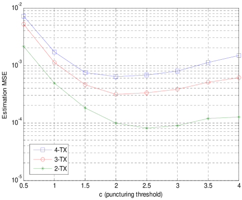
Figure 5: Threshold parameter $c$ optimization

In effectively whitening the correlated decision error, the constant $c$ is a crucial parameter that determines the number of selected symbols $N_{d}$ and thus controls the trade-off between the observation sample size and the amount of error correlation in the channel estimator. The existence of an optimum value for $c$ is also shown through the MSE simulation results of Fig. 5. Based on Fig. 5, we set $c=2$ for the $3\times 3$ and $4\times 4$ SM-MIMO-OFDM systems, and $c=2.5$ for the $2\times 2$ SM-MIMO-OFDM system.

Even with unbiased decision errors, the LMMSE estimator suffers performance degradation when the noise variance is mismatched. Let us quantify the MSE penalty associated with not accounting for the uncertainty inherent in the soft decisions in the form of increased noise variance. The LMMSE estimator failing to consider the soft decision error can be described as

$$\hat{\bf{w}}_{n}^{(r)} = {\bf{W}}_{n}^{(r)}{\bf{z}}_{n}^{(r)}$$ (55)

$${\bf{W}}_{n}^{(r)} = {\bf{R}}_{h}^{(r)}\widetilde{\bf{S}}_{n}^{H}\left({\widetilde{\bf{S}}_{n}{\bf{R}}_{h}^{(r)}\widetilde{\bf{S}}_{n}^{H}+\mathcal{N}_{o}{\bf{I}}_{N_{d}}}\right)^{-1}$$ (56)

$$= \left({\widetilde{\bf{S}}_{n}^{H}\widetilde{\bf{S}}_{n}+\mathcal{N}_{o}{\bf{R}}_{h}^{(r)-1}}\right)^{-1}\widetilde{\bf{S}}_{n}^{H}.$$

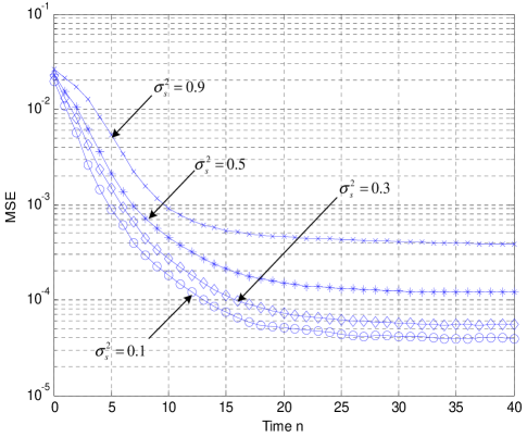
Figure 6: Open-loop channel estimation MSE for different values of $\sigma_{s}^{2}$ ($N_{d}=12$)

Utilizing (48) and denoting ${\bf\Delta}_{n}^{(r)}\buildrel\Delta\over{=}\hat{\bf{h}}_{n}^{(r)}-\hat{\bf{w}}_{n}^{(r)}$, the estimation error variance $\varepsilon_{w}^{2}$ of the estimator (56) can be shown to be

$$\varepsilon_{w}^{2}[n] = \sum\limits_{r=1}^{N_{r}}{E\left\{\|{\mathbf{h}}_{n}^{(r)}-\hat{\mathbf{w}}_{n}^{(r)}\|^{2}\right\}}$$ (57)

$$= \sum\limits_{r=1}^{N_{r}}{{\bf{tr}}{E\left\{{\|{{\bf{h}}_{n}^{(r)}-\left({\hat{\bf{h}}_{n}^{(r)}-{\bf{\Delta}}_{n}^{(r)}}\right)}\|^{2}}\right\}}}$$

$$= \varepsilon_{opt}^{2}[n]+\sum\limits_{r=1}^{N_{r}}{\bf{tr}}\left\{E\left\{{{\bf{h}}_{n}^{(r)}\hat{\bf{h}}_{n}^{(r)H}-\hat{\bf{w}}_{n}^{(r)}\hat{\bf{w}}_{n}^{(r)H}}\right.\right.$$

$$\left.\left.+\hat{\bf{w}}_{n}^{(r)}{\bf{h}}_{n}^{(r)H}-{\bf{h}}_{n}^{(r)}\hat{\bf{w}}_{n}^{(r)H}\right\}\right\}.$$

To simplify notation, the indices $r$ and $n$ are temporally dropped. As the number of iteration increases, the matrix inversions in (46) and (56) can be simplified as $\left({\widetilde{\bf{S}}^{H}\widetilde{\bf{S}}+{v}{\bf{R}}_{h}^{-1}}\right)^{-1}={\rm{diag}}[\,\,{{\rho_{1}}}/{{\left(\rho_{1}N_{d}({E_{s}+\sigma_{s}^{2}})+v\right)}}$,…,$\\ {{\rho_{N_{t}}}}/{{\left(\rho_{N_{t}}N_{d}({E_{s}+\sigma_{s}^{2}})+v\right)}}\,\,]\,\,$ and $\left({\widetilde{\bf{S}}^{H}\widetilde{\bf{S}}+\mathcal{N}_{o}{\bf{R}}_{h}^{-1}}\right)^{-1}={\rm{diag}}[{{\rho_{1}}}/{{\left(\rho_{1}N_{d}({E_{s}+\sigma_{s}^{2}})+\mathcal{N}_{o}\right)}}$,…,${{\rho_{N_{t}}}}/\left(\rho_{N_{t}}N_{d}({E_{s}+\sigma_{s}^{2}}\right)$ $\\ +\mathcal{N}_{o})]$, where the subscript for $\rho$ for the time being indicates the TX antenna. Also, noting $E\{{\hat{\bf{h}}({{\bf{h}}-\hat{\bf{h}}})^{H}}\}=0$ by the orthogonality principle, it can be shown that

$$\begin{array}[]{l}\,\,E\{{{\bf{h}}\hat{\bf{h}}^{H}}\}={\bf{R}}_{h}{\bf{S}}^{H}\widetilde{\bf{S}}\left({\widetilde{\bf{S}}^{H}\widetilde{\bf{S}}+{v}{\bf{R}}_{h}^{-1}}\right)^{-H}\\ \,\,={\rm{diag}}\left[\frac{{\rho_{1}^{2}N_{d}{E_{s}}}}{{\rho_{1}N_{d}\left({E_{s}+\sigma_{s}^{2}}\right)+v}},...,\frac{{\rho_{N_{t}}^{2}N_{d}{E_{s}}}}{{\rho_{N_{t}}N_{d}\left({E_{s}+\sigma_{s}^{2}}\right)+v}}\right]_{N_{t}\times N_{t}}.\end{array}$$ (60)

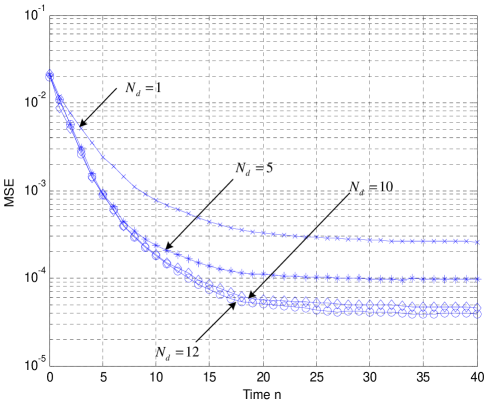
Figure 7: Open-loop channel estimation MSE depending on different values of $N_{d}$ ($\sigma_{s}^{2}=0.1$)

We also write

$$\begin{array}[]{l}E\{\hat{\bf{w}}\hat{\bf{w}}^{H}\}\\ =\left({\widetilde{\bf{S}}^{H}\widetilde{\bf{S}}+\mathcal{N}_{o}{\bf{R}}_{h}^{-1}}\right)^{-1}\widetilde{\bf{S}}^{H}\left({{\bf{SR}}_{h}{\bf{S}}^{H}+\mathcal{N}_{o}{\bf{I}}_{N_{d}}}\right)\\ \,\,\,\,\,\,\,\,\,\cdot\,\widetilde{\bf{S}}\left({\widetilde{\bf{S}}^{H}\widetilde{\bf{S}}+\mathcal{N}_{o}{\bf{R}}_{h}^{-1}}\right)^{-H}\\ ={\rm{diag}}\left[\frac{{\rho_{1}^{2}N_{d}\left({\rho_{1}N_{d}E_{s}^{2}+{\rho_{{}_{\Sigma}}}\sigma_{s}^{2}E_{s}+\mathcal{N}_{o}\left({E_{s}+\sigma_{s}^{2}}\right)}\right)}}{{\left({\rho_{1}N_{d}\left({E_{s}+\sigma_{s}^{2}}\right)+\mathcal{N}_{o}}\right)^{2}}},...,\right.\\ \,\,\,\,\,\,\,\,\,\left.\frac{{\rho_{N_{t}}^{2}N_{d}\left({\rho_{N_{t}}N_{d}E_{s}^{2}+{\rho_{{}_{\Sigma}}}\sigma_{s}^{2}E_{s}+\mathcal{N}_{o}\left({E_{s}+\sigma_{s}^{2}}\right)}\right)}}{{\left({\rho_{N_{t}}N_{d}\left({E_{s}+\sigma_{s}^{2}}\right)+\mathcal{N}_{o}}\right)^{2}}}\right]_{N_{t}\times N_{t}},\end{array}$$ (66)

where ${\rho_{{}_{\Sigma}}}={\sum\nolimits_{t=1}^{N_{t}}{\rho_{t}}}$. Finally, substituting (60) and (66) in (57) and also noting $E\{\hat{\bf{w}}{\bf{h}}^{H}\}=E\{{\bf{h}}\hat{\bf{w}}^{H}\}$, the MSE convergence behavior of the estimator (57) can be shown to be

$$\begin{array}[]{l}\displaystyle\mathop{\lim}\limits_{N_{d}\to\infty}\varepsilon_{w}^{2}[n]\\ \displaystyle=\varepsilon_{opt}^{2}[n]+\sum\limits_{r=1}^{N_{r}}{\frac{{\rho^{(r)}_{\Sigma}E_{s}}}{{E_{s}+\sigma_{s}^{2}[n]}}\left({1-\frac{{E_{s}}}{{E_{s}+\sigma_{s}^{2}[n]}}}\right)},\end{array}$$ (69)

from which it is easy to see that the mismatched MSE is an increasing function of the soft decision error variance $\sigma_{s}^{2}$.

To develop insights into the performance sensitivity off the sequentially updated channel estimator against the variations of the parameters $\sigma_{s}^{2}$ and $N_{d}$, we resort to an open-loop investigation. For this, the decision-feedback channel estimator is modified in such a way that unbiased soft decisions with various $\sigma_{s}^{2}$ and $N_{d}$ combinations are artificially generated for the channel estimator. A 7-iteration IDD receiver for the $2\times 2$ 16-QAM MIMO-OFDM system is used for this test, but instead of using actual feedback from the demappers and decoders, artificially generated soft-decisions are provided to the channel estimator of (27)-(30).

Fig. 6 and Fig. 7 show the MSE performance depending on the decision quality $\sigma_{s}^{2}$ and the number of feedback decisions $N_{d}$ with an assumption of uncorrelated feedback decisions. The signal power is fixed at $E_{s}=1$ and the channel SNR at 14 dB. With $N_{d}=12$, the packet error rate (PER) due to imperfect CSI became negligible when $\sigma_{s}^{2}\approx 0.1$. In Fig. 7, it is seen that reducing the number of feedback decisions, $N_{d}$, while fixing the decision quality causes the MSE to increase.

V Performance Evaluation

The proposed algorithm is investigated through an extrinsic information transfer (EXIT) chart analysis and packet error rate (PER) simulation. Performances are evaluated for $2\times 2$, $3\times 3$ and $4\times 4$ 16-QAM SM-MIMO-OFDM systems. The transmitter sends a packet with $1000$ bytes of information. The SISO MAP-demapper is used for the $2\times 2$ SM-MIMO-OFDM system, whereas the SISO MMSE-demapper is used for the $3\times 3$ and $4\times 4$ SM-MIMO-OFDM system [6] due to complexity. A rate-$1/2$ convolutional code is used with generator polynomials $g_{o}=133_{8}$ and $g_{1}=171_{8}$, complying with the IEEE 802.11n specifications [26]. The SOVA is used for decoding. The MIMO multi-path channel is modeled with an exponentially-decaying power profile with $T_{rms}=50ns$ uncorrelated across the TX-RX links established.

V-A EXIT and PER Performance Comparisons

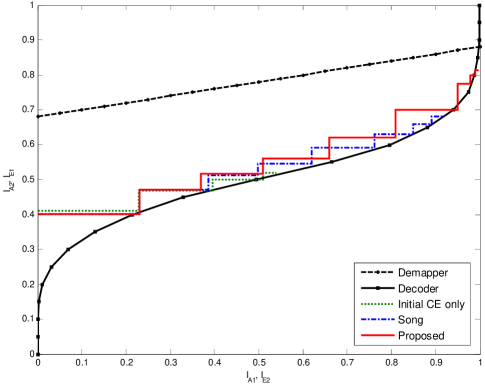
Figure 8: EXIT charts for the $2\times 2$ SM-MIMO-OFDM turbo receiver at SNR=14 dB

The EXIT chart is a well-established tool that allows the understanding of the average convergence behavior of the mutual information (MI) in iterative soft-information processing systems [28]. Fig. 8 shows the results of an EXIT chart analysis on various competing schemes. A $2\times 2$ SM-MIMO-OFDM system is used for this, and an SNR of 14 dB is chosen. $I_{A_{1}}$ and $I_{E_{1}}$ measure the MI at the input and output of the demapper, respectively, whereas $I_{A_{2}}$ and $I_{E_{2}}$ are the respective MI at the input and output of the decoder. At the next iteration stage, $I_{E_{1}}$ becomes $I_{A_{2}}$ and $I_{E_{2}}$ turns to $I_{A_{1}}$.

In the figure, the top-most curve indicates the average transfer function of MI through the demapper and the bottom-most curve is the same function for the decoder. Both the demapper and decoder EXIT chart curves correspond to Gaussian-distributed input LLRs, and the demapper EXIT curve is also based on the assumption of perfect channel estimation. The stair-case MI plots represent actual MI measured during IDD simulation runs and shows how the MI improves through the iterative process for three different channel estimation schemes. The gap between each stair-case MI trajectory and the demapper EXIT curve represents the performance loss due to imperfect-CSI. The solid stair-case line represents the proposed channel estimation algorithm. The dashed-line (labeled “Song”) corresponds to the Kalman channel estimator of [23] applied to the conventional-IDD setting (non-pipelined IDD with a demapper utilizing the noise-variance update of (32) with channel estimation using only the decoder output decision). The dotted line is for the demapper utilizing only the preamble-based initial channel estimation (following the IEEE 802.11n format, where a fixed number of initial preamble symbols in the high-throughput long training field is utilized). For the proposed scheme, the MI trajectory measurement is taken from the last demapper in the pipeline, as the last demapper block best reflects the quality of the final decisions.

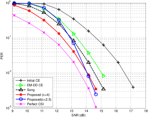
Figure 9: PERs with different channel estimators: 2x2 SM-MIMO-OFDM (7 iterations)

It is clear that the proposed punctured-feedback Kalman estimation with pipelined-IDD shows superior MI convergence characteristics. The scheme of [23] fails to improve MI beyond nine iterations. With the demapper utilizing only initial channel estimation, the trajectory fails to advance earlier in the iteration.

Fig. 9 shows PER performances of the receivers with different channel estimators in the $2\times 2$ SM-MIMO-OFDM system. Seven iterations are applied beyond which the iteration gain is plateaued. The performance gap between perfect CSI and preamble-based initial CE only is nearly 3 dB at low PERs. It can be seen that at low PER the proposed estimator almost compensates for the loss due to imperfect-CSI when the threshold parameter is set at $c=2.5$. Although the performance with small $c$ has inferior performance at low SNRs, the proposed Kalman CE curve with $c=2.5$ crosses the $c=4$ curve as SNR gets higher. The large $c$ is effective in averaging noise in low SNR, but allows relatively large correlated errors. As expected from the EXIT chart analysis results, the Kalman estimator of [23] that utilizes only the decoder output in a non-pipelined setting does not perform as well. As one of the algorithms considered for comparison, the decision-directed EM estimator (referred to as EM-DD here) introduced as a variant of the EM estimator in [19] is applied with $\hat{\bf{h}}_{o,n}^{(r)}=\left({\widetilde{\bf{S}}_{n}^{H}\widetilde{\bf{S}}_{n}}\right)^{-1}\widetilde{\bf{S}}_{n}^{H}{\bf{z}}_{n}^{(r)}$. In addition, the EM estimate is blended with the preamble-based channel estimate by a combining method (i.e., $\hat{{h}}_{n}^{(t,r)}=a_{n}\hat{h}_{preamble}^{(t,r)}+b_{n}\hat{h}_{o}^{(t,r)}[n]$) [20]. A method to find the combining coefficients $a_{n}$ and $b_{n}$ is discussed in [20]. The EM noise variance update method is presented in [19] as $\widehat{\mathcal{N}}_{o}[n]={1}/{{N_{r}N_{d}}}\sum\limits_{r=1}^{N_{r}}{\sum\limits_{d=0}^{N_{d}-1}\left({z_{n}^{(r)}-\widetilde{\bf{S}}_{n}\hat{\bf{h}}_{n}^{(r)}}\right)^{*}\left({z_{n}^{(r)}-\widetilde{\bf{S}}_{n}\hat{\bf{h}}_{n}^{(r)}}\right)}$. As can be seen, this scheme also does not perform as well as the proposed algorithm.

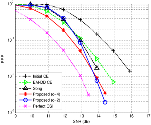
Figure 10: PERs with different channel estimators: 3x3 SM-MIMO-OFDM (7 iterations)

Fig. 10 and Fig. 11 show PER curves for $3\times 3$ SM-OFDM-OFDM and $4\times 4$ SM-OFDM-OFDM systems, respectively. These figures tell a consistent story. Namely, the initial-CE-only scheme suffers about a 3dB SNR loss relative to the perfect CSI case. The proposed schemes close this gap significantly, outperforming both the Kalman-based algorithm of [23] and the EM-based algorithm of [19]. As for the proposed channel estimation scheme, a more aggressive puncturing (corresponding to a lower $c$ value) tends to give a lower PER as SNR increases.

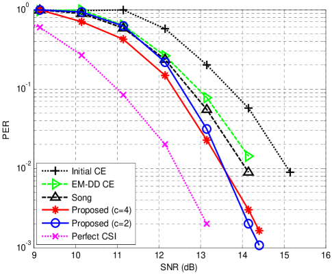
Figure 11: PERs with different channel estimators: 4x4 SM-MIMO-OFDM (9 iterations)

Before finishing this section, we briefly mention complexity. For all considered channel estimation schemes - the proposed, the Song method and the EM-DD scheme - implementation complexity largely arises from the matrix inversion operation. All schemes require matrix inversions of the same dimension. Consequently, the proposed method and the Song method require complexity that roughly grows as $2N_{r}\times O(N_{t}^{3})$ whereas the EM-DD requires complexity proportional to just $O(N_{t}^{3})$. This is due to the consequence that both our method and the Song method require matrix inversion for each receive antenna, whereas the EM-DD method needs matrix inversion just once and can be used for all receive antennas. The factor 2 accounts for the fact that two matrix inversions are required for each update of the Kalman gain in the proposed and Song methods.

VI Conclusions

A sequential soft-decision-directed channel estimation algorithm for MIMO-OFDM systems has been proposed for the specific pipelined turbo-receiver architecture. The algorithm deals with observation sample sets with varying levels of reliability. In coping with decision errors that propagate in the pipeline, we have introduced a novel method of innovating a correlated observation sequence via puncturing. Based on the refined innovation sequence, a Kalman-based estimator has been constructed. The proposed algorithm establishes improved Kalman-based channel estimation where the traditional innovations approach cannot create a true innovation sequence due to soft-decision error propagation. The EXIT chart, MSE analysis and PER simulation results have been used to validate the performance advantage of the proposed channel estimator.

Daejung Yoon received the B.S. and M.S. degrees in electrical engineering from the Kyungpook National University, Daegu, Korea, in 2003 and 2005, respectively. Currently, he is working toward the Ph.D. degree in electrical engineering at the University of Minnesota at Minneapolis. Since 2009, he has worked as a senior engineer in Samsung Information Systems America, San Jose, CA. His research interests are in the general areas of communication systems, advanced signal processing for digital communications and hard-disk signal processing.

Jaekyun Moon received a BSEE degree with high honor from the State University of New York at Stony Brook in 1984 and M.S. and Ph.D. degrees in the Electrical and Computer Engineering Department at Carnegie Mellon University in 1987 and 1990, respectively. In 1990, he joined the faculty of the Department of Electrical and Computer Engineering at the University of Minnesota, Twin Cities, as an Assistant Professor. He was promoted to a Tenured Associate Professor in 1995 and then to a Full Professor in 1999. Prof. Moon’s research interests are in the area of channel characterization, signal processing and coding for data storage and digital communication. His recent interests are in coding and equalization for interference-dominant channels. Prof. Moon was selected to receive the IEEE-Engineering Foundation Research Initiation Award in 1991 and received the NSF Reseacrh Initialtion Award in the same year. He received the 1994-1996 McKnight Land-Grant Professorship from the University of Minnesota. He also received the IBM Faculty Development Awards as well as the IBM Partnership Awards. He was awarded the National Storage Industry Consortium (NSIC) Technical Achievement Award for the invention of the maximum transition run (MTR) code, a widely-used error-control/modulation code in commercial storage systems. Prof. Moon served as Program Chair for the 1997 IEEE Magnetic Recording Conference. In 1998, he was a Visiting Professor at Seoul National University. He is also a past elected Chair of the Signal Processing for Storage Technical Committee of the IEEE Communications Society. In 2001, he co-founded Bermai, Inc., a fabless semiconductor start-up, and served as founding President and CTO. From 2004 to 2007, Prof. Moon worked as a consulting Chief Scientist for DSP Group, Inc. He served as a guest Editor for the 2001 IEEE J-SAC issue on Signal Processing for High Density Storage. He also served as an Editor for IEEE Transactions on Magnetics in the area of signal processing and coding for 2001-2006. While on leave from the University of Minnesota, he worked as Chief Technology Officer at Link-A-Media Devices Corp. in 2008. Prof. Moon joined KAIST as a Full Professor in 2009. He is an IEEE Fellow.

References

- [1] G. Caire, G. Taricco, and E. Biglieri, “Bit-interleaved coded modulation,” IEEE Trans. Inform. Theory, vol. 44, no. 3, pp. 927-946, May, 1998.
- [2] A. Tonello, “Space-time bit-interleaved coded modulation with an iterative decoding strategy,” Proc. of IEEE Vehicular Technology Conference, pp. 473-478, Boston, Sept., 2000.
- [3] D. Park and B. Lee, “Design criteria and performance of space-frequency bit-interleaved coded modulations in frequencyselective Rayleigh fading channels,” Journal of Commun. and Networks, vol. 5, no. 2, pp. 141-149, June, 2003.
- [4] C. Douillard, M. Jezequel, C. Berrou, A. Picart, P. Didier, and A. Glavieux, “Iterative correction of intersymbol interference: Turbo-equalization,” in European Trans. Telecomm., vol. 6, pp. 507–511, September 1995.
- [5] R. Koetter, A. Singer, and M. Tuchler, “Turbo equalization : an iterative equalization and decoding technique for coded data transmission,” IEEE Signal Processing Mag., vol. 21, pp. 67-80, Jan. 2004.
- [6] M. Tuchler, A. Singer, and R. Koetter, “Minimum mean square error equalization using a prori information,” IEEE Trans. Signal Processing, vol. 50, no. 3, pp. 673-683, Mar, 2002.
- [7] Y. Huang and J. Ritcey, “EXIT chart analysis of BICM-ID with imperfect channel state information,” IEEE Commun. Letters, vol. 7, no. 9, pp. 434-436, Sept., 2003.
- [8] Y. Huang and J. Ritcey, “16-QAM BICM-ID in fading channels with imperfect channel state information,” IEEE Trans. Wireless Commun., vol. 2, no. 5, pp. 1000-1007, Sept., 2003.
- [9] Y. Li, N. Seshadri, and S. Ariyavisitakul, “Channel estimation for OFDM systems with transmitter diversity in mobile wireless channels,” IEEE J. Select Areas Commun., vol. 17, no. 3, pp. 461-471, Mar., 1999.
- [10] Y. Li, L. Cimini, and N. Sollegberger, “Robust channels estimation for OFDM systems with rapid dispersive fading channels,” IEEE Trans. Commun., vol. 46, no. 7, pp. 902-915, Jul., 1998.
- [11] Y. Li, “Simplified channel estimation for OFDM systems with multiple transmit antennas,” IEEE Trans. Wireless Commun., vol. 1, no. 1, pp. 67-75, Jan., 2002.
- [12] X. Ma, L. Yang, and G. Giannakis, “Optimal training for MIMO frequency-selective fading channels,” IEEE Trans. Wireless Commun., vol. 4, no. 2, pp. 453-466, Mar., 2005.
- [13] B. Hassibi and B. Hochwald, “Optimal training in space time systems,” Proc. 34th Asilomar Conf. on Signals, Systems and Computers, pp. 743-747, Oct., 2000.
- [14] X. Deng, A. Haimovich, and J. Garcia-Frias, “Decision directed iterative channel estimation for MIMO systems,” Proc. IEEE Int. Conf. Commun., vol. 4, pp. 2326-2329, Anchorage, AK, May, 2003.
- [15] J. Gao and H. Liu, “Decision-directed estimation of MIMO time-varying Rayleigh fading channels,” IEEE Trans. Wireless Commun., vol. 4, no. 4, pp. 1412-1417, Jul., 2005.
- [16] M. Loncar, R. Muller, J. Wehinger, and T. Abe, “Iterative joint detection, decoding, and channel estimation for dual antenna arrays in frequency selective fading,” Proc. Int. Symposium on Wireless Personal Multimedia Commun., Honolulu, HI, Oct., 2002.
- [17] M. Sandell, C. Luschi, P. Strauch, and R. Yan, “Iterative channel estimation using soft decision feedback,” Proc. Globecom, vol. 6, pp. 3728-3733, Sydney, Australia, Nov., 1998.
- [18] M. Tuchler, R. Otnes, and A. Schmidbauer, “Performance of soft iterative channel estimation in turbo equalizer,” Proc. IEEE ICC2002 Int. Conf. vol. 3, pp. 1858-1862, New York, NY, Apr. 2002.
- [19] X. Wautelet, C. Herzet, A. Dejonghe, J. Louveaux, and L. Vandendorpe, “Comparision of EM-based algorithms for MIMO channel estimation,” IEEE Trans. Commun., vol. 55, no. 1, pp. 216-226, Jan., 2007.
- [20] M. Kobayashi, J. Boutros, and G. Caire, “Successive interference cancellation with SISO decoding and EM channel estimation,” IEEE J. Select Areas Commun., vol. 19, no. 8, pp. 1450-1460, Aug., 2001.
- [21] M. Khalighi and J. Boutros, “Semi-blind channel estimation using the EM algorithm in iterative MIMO APP detectors,” IEEE Wireless Commun., vol. 5, no. 11, pp. 3165-3173, Nov., 2006.
- [22] S. Song, A. Singer, and K. Sung, “Soft input channel estimation for turbo equalization,” IEEE Trans. Sig. Processing, vol. 52, no. 10, pp. 2885-2894, Oct., 2004.
- [23] S. Song, A. Singer, and K. Sung, “Turbo equalization with unknown channel,” in Proc. IEEE Int. Conf. Acoustics, Speech, and Sig. Processing ICASSP, vol. 3, pp. 2805-2808, Orlando, FL, May 2002.
- [24] S. Abbasfar, “Turbo-like codes; design for high speed decoding,” Springer, Netherlands, 2007.
- [25] S. Lee, N. Shanbhag, and A. Singer, “Area-efficient high-throughput VLSI architecture for MAP-based turbo equalizer,” Proc. IEEE signal procssing system: design and implementation pp. 87-92, Aug. 2003, Seoul, Korea.
- [26] IEEE P802.11n/D1.0 : Draft Amendment to STANDARD FOR 2 Information Technology-Telecommunications and 3 information exchange between systems-Local and 4 Metropolitan networks-Specific requirements-Part 5 11: Wireless LAN Medium Access Control (MAC) 6 and Physical Layer (PHY) specifications: 7 Enhancements for Higher Throughput.
- [27] H. Stark and J. Woods, “Probability and random processes with applications to signal processing,” USR, NJ, Prentice-Hall, 2002.
- [28] S. Brink, “Designing iterative decoding schemes with the extrinsic information transfer chart,” Int. J. Electron. Commun., vol. 54, No. 6, pp. 389-398, Nov. 2000.
- [29] J. Hagenauer and P. Hoeher, “A Viterbi Algorithm with Soft-Decision Outputs and its Applications,” Globecom 1989, vol. 3, pp. 1680-1686, Dallas,TX, Nov., 1989
- [30] S. Kay, “Fundamentals of statistical signal processing-estimation theory,” Englewood Cliffs, NJ, Prentice-Hall, 1993.