Quantum Hall effects in fast rotating Fermi gases with anisotropic dipolar interaction

Abstract

We investigate fast rotating quasi-two-dimensional dipolar Fermi gases in the quantum Hall regime. By tuning the direction of the dipole moments with respect to the $z$-axis, the dipole-dipole interaction becomes anisotropic in the $x$-$y$ plane. For a soft confining potential we find that, as we tilt the angle of the dipole moments, the system evolves from a $\nu=1/3$ Laughlin state with dipoles being polarized along the $z$ axis to a series of ground states characterized by distinct mean total angular momentum, and finally to an anisotropic integer quantum Hall state. During the transition from the fractional regime to the integer regime, we find that the density profile of the system exhibits crystal-like structures. We map out the ground states as a function of the tilt angle and the confining potential, revealing the competition of the isotropic confining potential and both the isotropic and anisotropic components of the dipole-dipole interaction.

I Introduction

The quest for quantum computer with intrinsic fault tolerance spurs recent interest in searching for exotic fractional quantum Hall (FQH) states that support non-Abelian anyons nayak08 . While it is easy to write down a trial wave function with highly nontrivial statistics, the realization of it in two-dimensional electron gases (2DEGs) is not simple. Apart from the technical difficulties of sample preparation and low operating temperature, the lack of effective control on the interaction between particles is a major concern. In a realistic 2DEG, electrons interact via long-range Coulomb interaction, which may be modified due to the presence of an adjacent gate in the case of graphene or the effect of Landau level (LL) mixing, which introduces effective three-body interaction (among others). In particular, recent theoretical and experimental studies bishara09 ; xia10 ; wojs10 ; rezayi11 suggest that the perturbative modification of the interparticle interaction can have significant effects on the stability of FQH states. Therefore, the question of how topological order evolves with interparticle interaction remains an interesting question with growing experimental capabilities of controlling microscopic parameters.

Ultracold atomic gases provide an ideal platform for simulating quantum many-body systems bloch . The realizations of FQH states in ultracold Fermi gases have been discussed in the presence of, for example, a rapidly rotating trap cooper ; fetter or a laser-induced geometric gauge field lin . For identical fermions, $s$-wave interactions vanish due to the Pauli exclusion principle. Unless in the resonance regime, $p$-wave interactions in a single-component Fermi gas are typical very small. Nevertheless, significant interactions can still be introduced by using atoms or molecules with strong dipole-dipole interactions lu ; ye1 ; ye2 . The FQH effects in a two-dimensional (2D) dipolar Fermi gas with isotropic dipole-dipole interaction have been studied in Refs. bara ; Lewenstein . The system has been shown to undergo transitions from an integer quantum Hall (IQH) state to a $\nu=1/3$ Laughlin state, and to a Wigner-crystal state by increasing the rotation frequency. However, we are not aware of any work on the FQH effects in the presence of anisotropic interaction, when the dipoles are not oriented along the rotation axis.

In the present work, we study the FQH effects in a fast rotating quasi-2D gas of polarized fermionic dipoles. By tilting the direction of the dipole moments with respect to the rotation axis, we can tune the dipole-dipole interaction to be anisotropic on the plane of motion. Starting from a Laughlin state with isotropic dipolar interaction, we investigate the ground state properties by varying the tilt angle of the dipole moments. We find that for small tilt angle the ground state can be approximately described by a FQH state. However, as one further increases the tilt angle, the ground state deviates from the FQH state significantly such that a crystal-like pattern emerges in the density profile of the gas. The ground state of the system eventually becomes an IQH state when dipole moments are aligned in the 2D plane. For a soft confining potential, the IQH state is noticeably anisotropic. We map out the phase diagram in the parameter space spanned by the tilt angle and the strength of the confining potential. The results can be explained by the competition of the isotropic confining potential and both the isotropic and anisotropic components of the dipole-dipole interaction.

This paper is organized as follows. In Sec. II, we present our model and calculation for relevant matrix elements of the model Hamiltonian. Section III briefly covers the FQH states with isotropic dipolar interaction for later comparisons. In Sec IV we investigate the ground state structure in the presence of anisotropic dipole-dipole interaction in a weak confining potential. The full phase diagram is presented in Sec. V. We conclude our discussions in Sec. VI.

II Model

We consider a system of $N$ spin polarized fermionic dipoles trapped in an axially symmetric potential

$$U({\mathbf{r}})=\frac{1}{2}\mu(\omega^{2}x^{2}+\omega^{2}y^{2}+\omega_{z}^{2}z^{2}),$$

where $\mu$ is the mass of the particle, $\omega$ and $\omega_{z}$ are the radial and axial trap frequencies, respectively. The trapping potential rotates rapidly around the $z$-axis with an angular frequency $\Omega$ ($<\omega$). We further assume that the dipole moments $d$ of all particles are polarized by an external orienting field which is at an angle $\theta$ about the $z$-axis. Since the $s$-wave collisional interaction vanishes for spin polarized fermions, particles only interact with each other via a dipole-dipole interaction. If the orienting field corotates with the trapping potential, the dipolar interaction becomes time-independent in the rotating frame, i.e.,

$$\mathcal{V}(\mathbf{r})=c_{d}V_{\theta}^{\mathrm{(3D)}}({\mathbf{r}}),$$

where $c_{d}=d^{2}/(4\pi\varepsilon_{0})$ or $\mu_{0}d^{2}/(4\pi)$ for, respectively, electric or magnetic dipoles, with $\varepsilon_{0}$ ($\mu_{0}$) being the vacuum permittivity (permeability). The spatial dependence of ${\cal V}({\mathbf{r}})$ can be described by

$$V_{\theta}^{\mathrm{(3D)}}(\mathbf{r})=\frac{1}{r^{5}}\,\left[r^{2}-3(z\cos\theta+x\sin\theta)^{2}\right].$$

Here, without loss of generality, we have assumed that the dipole moments are polarized in the $x$-$z$ plane of the rotating frame. We can tune the dipolar interaction by introducing a tilt angle $\theta$ such that $V_{\theta}^{\mathrm{(3D)}}({\mathbf{r}})$ is isotropic (anisotropic) on $x$-$y$plane for $\theta=0$ ($\theta\neq 0$). In the rotating frame, the Hamiltonian of the system becomes

$$H_{\mathrm{3D}}=\sum_{i}\left[\frac{{\mathbf{p}}_{i}^{2}}{2\mu}+U({\mathbf{r}}_{i})-\Omega L_{i}^{z}\right]+c_{d}\sum_{i<j}V_{\theta}^{\mathrm{(3D)}}({\mathbf{r}}_{i}-{\mathbf{r}}_{j}),$$

(1)

where $L^{z}=xp_{y}-yp_{x}$ is the $z$ component of the orbital angular momentum.

Under the condition $\omega_{z}\gg\omega$, the system can be regarded as quasi-2D. As a result, the motion of all particles along the $z$-axis is frozen to the ground state of the axial harmonic oscillator, with a wave function $\phi_{z}(z)=\pi^{-1/4}q^{-1/2}e^{-z^{2}/(2q^{2})}$, where $q=\sqrt{\hbar/(\mu\omega_{z})}$. Integrating out the variable $z$ from Eq. (1), we obtain the Hamiltonian for the quasi-2D system as

$$H_{\mathrm{2D}} = \sum_{i}\left[\frac{({\mathbf{p}}_{i}-\mu\omega\hat{\mathbf{e}}_{z}\times{\bm{\rho}}_{i})^{2}}{2\mu}+\hbar(\omega-\Omega)L_{i}^{z}\right]$$ (2)

$$+c_{d}\sum_{i<j}V_{\theta}^{\mathrm{(2D)}}({\bm{\rho}}_{i}-{\bm{\rho}}_{j}).$$

where ${\bm{\rho}}=(x,y)$, $\hat{\mathbf{e}}_{z}$ is the unit vector along the $z$-axis and

$$V_{\theta}^{\rm(2D)}({\bm{\rho}})=\frac{1}{(2\pi q^{2})^{1/2}}\int dze^{-z^{2}/(2q^{2})}V_{\theta}^{(3D)}({\bm{\rho}},z).$$ (3)

The first term on the righthand side of Eq. (2) represents the single-particle Fock-Darwin Hamiltonian in the symmetric gauge Fock ; Darwin , which can be solved exactly to yield eigenenergies fetter

$$\hbar(\omega-\Omega)n_{+}+\hbar(\omega+\Omega)n_{-}+\hbar\omega,$$ (4)

known as the Fock-Darwin levels, where the quantum numbers $n_{+}$ and $n_{-}$ are two non-negative integers. In the fast rotating limit $\Omega\rightarrow\omega$, the Fock-Darwin levels mimic the LLs with a level spacing $2\hbar\Omega$. Throughout this work, we assume that the interaction energy is much smaller than the LL spacing, such that particles only occupy the highly degenerate lowest Landau level (LLL).

To proceed further, it is convenient to introduce a set of dimensionless units: $\hbar$ for angular momentum, $\ell=\sqrt{\hbar/(2\mu\omega)}$ for length, and $c_{d}/\ell^{3}$ for energy. The wave function of the LLL can then be expressed as

$$\psi_{m}(\rho,\varphi)=\frac{\rho^{m}e^{im\varphi}e^{-\rho^{2}/4}}{\sqrt{2\pi 2^{m}m!}}\quad(m\geq 0),$$

describing a state with an angular momentum $m\hbar$. Within the LLL formalism, the Hamiltonian (2) in the second quantization reads

$$H=\alpha L^{z}+\frac{1}{2}\sum_{m_{1}m_{2}m_{3}m_{4}}V_{1234}(\theta)f_{m_{1}}^{{\dagger}}f_{m_{2}}^{{\dagger}}f_{m_{4}}f_{m_{3}},$$ (5)

where $f_{m}^{{\dagger}}$ is the fermion creation operator that creates a particle in state $\psi_{m}$ and $L^{z}=\sum_{m}mf_{m}^{{\dagger}}f_{m}$ the total angular momentum. The dimensionless quantity $\alpha=\hbar(\omega-\Omega)\ell^{3}/c_{d}$ characterizes the relative strength of confining potential with respect to interaction. In the presence of anisotropy, the interaction matrix elements are

$$V_{1234}(\theta) = \int d{\bm{\rho}}_{1}d{\bm{\rho}}_{2}\psi_{m_{1}}^{\ast}({\bm{\rho}}_{1})\psi_{m_{2}}^{\ast}({\bm{\rho}}_{2})V_{\theta}^{\mathrm{(2D)}}({\bm{\rho}}_{1}-{\bm{\rho}}_{2})\psi_{m_{3}}({\bm{\rho}}_{1})\psi_{m_{4}}({\bm{\rho}}_{2})$$ (6)

$$= {\cal A}_{1234}\left[\frac{3\cos^{2}\theta-1}{2}\left(\frac{8}{3}{\cal J}_{1234}-4{\cal K}_{1234}\right)\delta_{m_{1}+m_{2},m_{3}+m_{4}}+\sin^{2}\theta{\cal K}_{1234}\delta_{m_{1}+m_{2},m_{3}+m_{4}\pm 2}\right],$$

where

$${\cal A}_{1234}=\frac{1}{2\sqrt{2\pi}q}\frac{i^{|m_{3}-m_{1}|-|m_{4}-m_{2}|}}{2^{(|m_{3}-m_{1}|+|m_{4}-m_{2}|)/2}}\sqrt{\frac{[m^{<}_{13}]![m^{<}_{24}]!}{[m^{>}_{13}]![m^{>}_{24}]!}},$$

$${\cal J}_{1234} = \int d\rho\rho^{|m_{3}-m_{1}|+|m_{4}-m_{2}|+1}e^{-\rho^{2}}$$

$$\!\!\!\!\times L_{m_{13}^{<}}^{|m_{3}-m_{1}|}\!\left(\frac{\rho^{2}}{2}\right)L_{m_{24}^{<}}^{|m_{4}-m_{2}|}\!\left(\frac{\rho^{2}}{2}\right),$$

$${\cal K}_{1234} = q\sqrt{\frac{\pi}{2}}\int d\rho\rho^{|m_{3}-m_{1}|+|m_{4}-m_{2}|+2}e^{-\rho^{2}+q^{2}\rho^{2}/2}$$

$$\!\!\!\!\times L_{m_{13}^{<}}^{|m_{3}-m_{1}|}\!\left(\frac{\rho^{2}}{2}\right)L_{m_{24}^{<}}^{|m_{4}-m_{2}|}\!\left(\frac{\rho^{2}}{2}\right){\rm erfc}\!\left(\frac{q\rho}{\sqrt{2}}\right),$$

where $m_{ij}^{<}=\mathrm{min}(m_{i},m_{j})$ and $m_{ij}^{>}=\mathrm{max}(m_{i},m_{j})$. $L_{m}^{n}(\cdot)$ is the associated Laguerre polynomial and $\mathrm{erfc}(\cdot)$ is the complementary error function. Clearly, for $\theta=0$ $V_{1234}$ is nonzero only when $m_{1}+m_{2}-m_{3}-m_{4}=0$, indicating that the total angular momentum $L_{z}$ is conserved in the isotropic case. However, when the interaction becomes anisotropic ($\theta\neq 0$), $V_{1234}$ are nonzero when $m_{1}+m_{2}-m_{3}-m_{4}=0$ or $\pm 2$.

Hamiltonian (5) contains three parameters: the total number of particles $N=\sum_{m}f_{m}^{{\dagger}}f_{m}$, the relative strength of the confining potential $\alpha$, and the tilt angle $\theta$ of the dipole moment. In the following sections, we will explore the quantum states of the system in the parameter space $(N,\theta,\alpha)$. Our main focus is on the parameter ranges of $N\leq 10$, $0\leq\theta\leq\frac{\pi}{2}$, and $0.01\leq\alpha\leq 0.1$. Unless otherwise stated, the value of $q$ is chosen to be $0.01\ell$.

III Quantum Hall states with isotropic dipolar interaction

Let us first assume that the dipolar interaction is isotropic in the $x$-$y$ plane, which corresponds to $\theta=0$ in the Hamiltonian (5). In this case, the total angular momentum is conserved. Therefore, one may numerically diagonalize the Hamiltonian (5) in the subspace of a given total angular momentum $M$ to obtain

$$H\left|\Phi^{(N)}_{M,n}\right\rangle=E^{(N)}_{M,n}\left|\Phi^{(N)}_{M,n}\right\rangle,$$ (7)

where $E^{(N)}_{M,n}$ and $\left|\Phi^{(N)}_{M,n}\right\rangle$ are eigenenergies and eigenstates, respectively. The index $n$ labels the state in the subspace of total angular momentum $M$ with increasing eigenenergy, i.e., $n=0$ for the lowest energy state, $n=1$ for the first excited states, etc. We emphasize that we present a numerically exact treatment of the dipolar interaction potential for a quasi-2D system with finite wave-function spread along the perpendicular direction, while the ideal 2D case has been studied previously Lewenstein .

Table 1: Magic numbers in an isotropic $N=10$ system with various $q$s. The magic numbers obtained from the composite fermion theory are included for comparison.

CF	45		55		63		69		77		83		90			97	103	111	117	125	135
$q=0.5$	45	52		59		66	69	73	77	80		85	90	93		97	103	111	117	125	135
$q=0.1$	45	52		59		66		73	77	80		85	90	93	95		103	111	117	125	135
$q=0.01$	45	52		59		66		73	77	80		85	90	93	95		103	111	117	125	135

In Fig. 1, we plot the eigenenergy versus the total angular momentum for $N=6$ and $\alpha=0$. As a guide to the eyes, we have connected the lowest energy state in each total angular momentum subspace by a piecewise straight line, on which a series of shoulders are visible. The first state on the each shoulder, where a downward cusp appears in the spectrum, represents a possible candidate for the global ground state of the system with increasing $\alpha$. For a given $\alpha\neq 0$, only one of these states is the global ground state of the system; the corresponding total angular momentum is so called a magic number. The properties of these states have been studied extensively. Laughlin first noticed that the lowest-energy state of the $M=3N(N-1)/2$ is closely related to the fractional quantum Hall effect Laughlinc . To translate these numbers into asymptotic filling factors in the thermodynamic limit, Girvin and Jach proposed an explicit expression for these states in the finite system Girvinb ,

$$\nu=\frac{L_{0}}{M},$$ (8)

where $L_{0}=N(N-1)/2$. In the context of quantum dots, Jain and Kawamura proposed an explanation of the magic numbers using the theory of composite fermions Jaina ; Jainb , which has been further discussed in later works Seki ; Maksym ; Landman . We list the magic numbers of our quasi-2D model for $N=10$ in Table 1 for several choices of $q$. For small $q$ up to 0.1, our results are consistent with the results in 2D rotating Fermi gases with isotropic dipolar interaction studied earlier by Osterloh et al Lewenstein . However, for larger $q$ we observe a few discrepancies. Interestingly, the magic numbers 69 and 97, not showing for small $q$, are consistent with the prediction of the composite fermion theory.

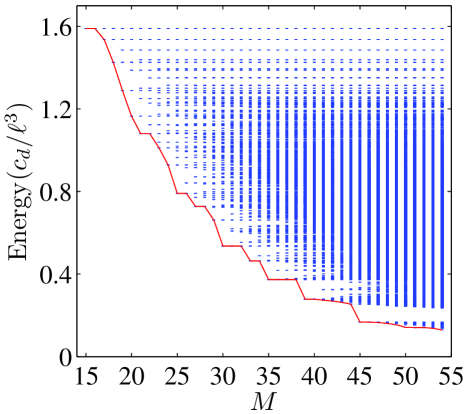
Figure 1: (Color online) Energy spectrum of Hamiltonian (5) with $N=6$, $\alpha=0$, and $\theta=0$. The solid (red) line connects the lowest energy state in each total angular momentum subspace as a guide to the eyes. The smallest angular momentum state on the each shoulder of the line may become the global ground state of the system as $\alpha$ varies.

IV Quantum Hall states with anisotropic interaction

Now we turn to the study of the quantum states in systems with anisotropic dipolar interaction. Since the total angular momentum $L^{z}$ is no longer conserved, one has to numerically diagonalize the Hamiltonian (5) in much larger Hilbert spaces. In practice, one may truncate the Hilbert space by introducing a cutoff, $m_{\rm cut}$, to the angular momentum $m$, such that the diagonalization procedures are carried out in the space constructed from $\psi_{m}$s with $m\leq m_{\rm cut}$. We have chosen a sufficiently large $m_{\rm cut}$ such that our results presented in this work are not the choice of $m_{\rm cut}$. In numerical diagonalization, we take advantages of the fact that dipole-dipole interaction only couples angular momentum subspaces that differ by an even angular momentum and diagonalize in the Hilbert space spanned by odd and even angular momentum states separately.

For a given set of parameters $(N,\alpha,\theta)$, the ground state wave function of the system is denoted by $\left|\Psi^{(N)}(\alpha,\theta)\right\rangle$ with the ground state energy $E^{(N)}(\alpha,\theta)$. Throughout this section, the strength of the confining potential is fixed at $\alpha=0.01$, such that the ground state is a $\nu=1/3$ Laughlin state for $\theta=0$. The dependence of the results on $\alpha$ will be discussed in the next section. Due to the large size of the Hilbert space involved in the numerical diagonalization, We study systems of up to $N=8$ fermions.

IV.1 State transitions induced by varying $\theta$

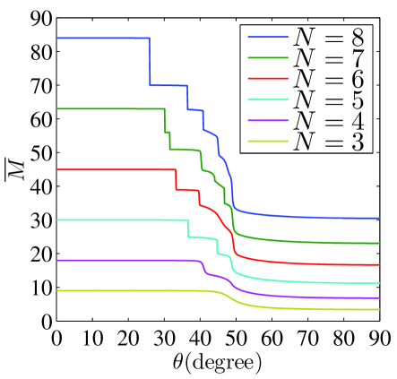
Figure 2: (Color online) Mean total angular momentum $\overline{M}$ versus the tilt angle $\theta$ for $\alpha=0.01$ in systems with various sizes up to $N=8$. For sufficiently large number of particles ($N\geq 5$), plateaus corresponding to distinct ground states develop on the curves.

Even though the total angular momentum $L^{z}$ is no longer a good quantum number, its mean value,

$$\overline{M}=\left\langle\Psi^{(N)}(\alpha,\theta)\right|L^{z}\left|\Psi^{(N)}(\alpha,\theta)\right\rangle,$$

can be defined and we will see that it is sufficient to characterize the ground state of a system. In Fig. 2, we plot the $\theta$ dependence of $\overline{M}$ for systems with $N\leq 8$. We find that $\overline{M}$ always decreases with $\theta$. As will be shown, this monotonically decreasing behavior of $\overline{M}(\theta)$ is because the dipolar interaction becomes less repulsive as $\theta$ is increased, which reduces the size of the system Laughlinb . Interestingly, for sufficiently large number of particles ($N\geq 5$), plateaus develop on the $\overline{M}(\theta)$ curves. Roughly speaking, for $\theta\lesssim 40^{\circ}$ the mean total angular momentum decreases abruptly from one plateau to another as the tilt angle is increased, signaling sharp transitions between ground states with distinct properties at various $\theta$. For a concrete example, we examine in detail the transitions for the system of $N=6$. The sudden drops of $\overline{M}$ are observed as

$$\overline{M}:\quad 45\;{\stackrel{{\scriptstyle 33.3^{\circ}}}{{\longrightarrow}}}\;39.0\;{\stackrel{{\scriptstyle 39.9^{\circ}}}{{\longrightarrow}}}\;34.89,$$ (9)

where the numbers above the two arrows denote the critical tilt angles. From the analysis presented in Sec. III, the first and second plateaus clearly correspond to the fractional quantum Hall states with filling factors $\nu=1/3$ and $5/13$, respectively, in the notation define in Eq. (8) by Girvin and Jach Girvinb . The third plateau has an mean total angular momentum of 34.89, which is 0.3% smaller than $35$, indicating that it mainly contains the FQH state with filling factor $\nu=3/7$. As one further increases $\theta$, $\overline{M}$ decreases smoothly toward an asymptotic value of $17$ at $\theta=90^{\circ}$. As shown in Fig. 2, similar features also appear in the systems with $N=5$, $7$ and $8$. For $N=3$ and $4$, however, $\overline{M}$ always varies smoothly, consistent with the expectation that quantum phase transitions happen only in thermodynamically large systems; the absence of the sharp steps for $N<5$ is the normal finite-size artifact.

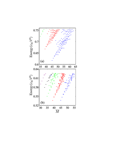
Figure 3: (Color online) Low-lying energy spectrum for an $N=6$ system with $\alpha=0.01$ and a tilt angle of (a) $\theta=0^{\circ}$ and (b) $33.3^{\circ}$. Distinct colors are used to specify different energy-level clusters, which can be regarded as chiral excitations of the corresponding lowest-energy state.

To gain insight into those transitions, we examine the energy spectrum of the system. In Fig. 3, we plot the low-lying energy levels versus the mean total angular momentum for $N=6$ for the isotropic and the anisotropic cases. In the isotropic case ($\theta=0$), the mean total angular momentum $\overline{M}$ is simply the total angular momentum $L^{Z}$, which is a good quantum number. In both cases, energy levels group into clusters which are plotted with different colors. For convenience, we shall refer to each energy cluster using the angular momentum of the lowest energy level in the cluster. Even though the boundary between two adjacent clusters are not well defined for high-energy states, the lowest ones are clearly well separated. In Fig. 3(a), we choose the range in which three energy-level clusters are visible. Among them, the lowest energy state in cluster-$45$ represents the ground state of the system for $\theta=0$. This is the 6-particle Laughlin state as discussed in Sec. III. Apart from its mean total angular momentum, we can also observe the feature of a Laughlin state also in the low-energy spectrum. First of all, the low-lying excitations are chiral, appearing only on the side of $\overline{M}>45$. In particular, at roughly $\overline{M}=46$ and $47$, we find one and two states, respectively. They can be interpreted as the edge excitations of the ground state droplet, with their wave functions approximated by the ground state wave function multiplied by a symmetric polynomial of the corresponding degree. Near $\overline{M}=48$, we expect three low-lying states but only find two; however, there is another level well above (near 0.7), presumably due to the influence of the cutoff in the momentum space. The series of numbers of the low-lying states is consistent with the chiral Luttinger liquid theory and signifies the topological order of the corresponding ground state 7 .

As one increases the tilt angle $\theta$, all energy-level clusters move downward to lower energies because the dipolar interaction becomes less repulsive. Nevertheless, the counting of the low-lying excitations remains robust, suggesting the topological order is not destroyed by small anisotropy, as shown in Fig. 3(b). In addition, the clusters with lower angular momentum move faster than those with higher angular momentum, hence, for example, the lowest energy state in cluster-$39$ becomes the ground state of the system at $\theta=33.3^{\circ}$. As one further increases $\theta$, the lowest energy state in cluster-35 will become the ground state of the system. They have different low-energy excitation structure from that of the $\overline{M}=45$ ground state. In the case of the cluster-$39$, in particular, there are two chiral excitations at $\Delta\overline{M}\approx 1$, clearly different from the Laughlin case.

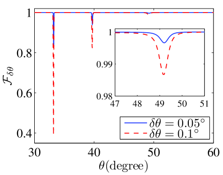
Figure 4: (Color online) Fidelity ${\cal F}_{\delta\theta}$, as defined in Eq. (10), as a function of $\theta$ for $N=6$ and $\alpha=0.01$. The inset magnifies the fidelity in the vicinity of the small dip around $\theta=49.3^{\circ}$.

The phase transitions induce by tuning anisotropy can be further confirmed by calculating the fidelity of the ground state wave function quan ; gusj ,

$${\cal F}_{\delta\theta}=\left|\left\langle\Psi^{(N)}(\alpha,\theta)\right.\left|\Psi^{(N)}(\alpha,\theta+\delta\theta)\right\rangle\right|,$$ (10)

where $\delta\theta$ is a small quantity. The fidelity $\cal F$ measures the similarity between two adjacent states in the parameter space gusj . In the bulk of a single quantum phase, two states close in the parameter space have wave functions that are only perturbatively different, hence ${\cal F}_{\delta\theta}$ is close to unity for sufficiently small $\delta\theta$. Near the phase boundary, two states that are close in the parameter space can have very different structure in their wave functions, therefore the fidelity can drop sharply in the quantum critical region, signaling a quantum phase transition in the thermodynamic limit. In Fig. 4, we plot the $\theta$ dependence of ${\cal F}_{\delta\theta}$ for a systems with $N=6$ particles. Two transition points can be clearly identified and the critical $\theta$ values are consistent with those obtained in Fig. 2. A closer look at the ${\cal F}_{\delta\theta}(\theta)$ (inset of Fig. 4) further reveals that there exists a third dip at $\theta\simeq 49.3^{\circ}$. The comparison of the fidelity ${\cal F}_{\delta\theta}$ for two different $\delta\theta$s indicates that the similarity of the ground states decreases with the increasing distance between the parameter $\delta\theta$ near the dip.

IV.2 Structure of the ground state wave function with anisotropic interaction

To reveal the structure of the ground state wave function $\left|\Psi^{(N)}(\alpha,\theta)\right\rangle$, let us calculate the overlap integral

$${\cal O}_{M,n}^{(N)}(\alpha,\theta)=\left|\left\langle\Phi^{(N)}_{M,n}\right|\left.\Psi^{(N)}(\alpha,\theta)\right\rangle\right|$$ (11)

between the isotropic and anisotropic ground states. Again, we present the data of the system with $N=6$ particles. Figure 5 shows the dependence of ${\cal O}_{M,0}^{(N)}$ on anisotropy for $M=45$, 39, 35, and $15$. As can be seen, the $\theta$-axis is roughly divided into four regions, the boundaries of which coincide with the three dips of the fidelity in Fig 4.

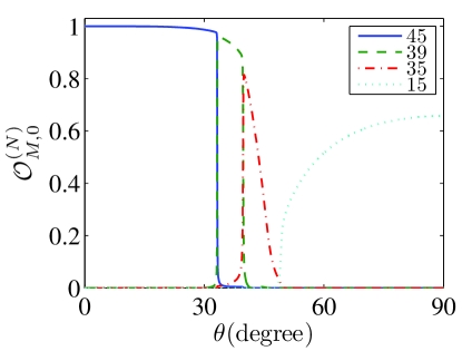
Figure 5: (Color online) Overlap integral ${\cal O}^{(6)}_{M,0}$ [Eq. (11)] versus $\theta$ for $M=45$ ($\nu=1/3$ Laughlin state), 39, 35, and 15 (IQH state) in the $N=6$ system with $\alpha=0.01$.

In the first region $\theta<33.2^{\circ}$, the overlap ${\cal O}_{45,0}^{(6)}$ is greater than $0.974$, which indicates that the dominate contribution to the ground state wave function comes from the Laughlin state $\left|\Phi^{(6)}_{45,0}\right\rangle$. Nevertheless, close to the right boundary of this region, several states in $M=47$ and $43$ manifolds are mixed into the ground state wave function, such that ${\cal O}^{(6)}_{45,0}$ drops notably. The ground state wave function in region $33.3^{\circ}<\theta<39.6^{\circ}$ mainly contains the states from $M=43,41,39$, and $37$ manifolds. Particularly, the state $\left|\Phi^{(6)}_{39,0}\right\rangle$ provides the largest contribution to the ground state with $0.858\leq{\cal O}^{(6)}_{39,0}\leq 0.96$.

In the region $39.8^{\circ}<\theta<49.3^{\circ}$, the situation is much more complicated compared to those in the first two regions. At the left boundary, ${\cal O}_{35,0}^{(6)}$ is as high as $0.814$, but it quickly drops to close to zero as the right boundary is approached. In fact, many states from $M=21$ to $37$ in the isotropic case contribute collectively to the ground state wave function. As a result, complicated structures are developed in the density profile of the system. In Fig. 6, we present four typical patterns in the density profiles

$$\varrho(x,y) = \sum_{mm^{\prime}}\left\langle\Psi^{(N)}(\alpha,\theta)\right|f_{m}^{\dagger}f_{m^{\prime}}\left|\Psi^{(N)}(\alpha,\theta)\right\rangle$$ (12)

$$\quad\times\psi_{m}^{*}(x,y)\psi_{m^{\prime}}(x,y)$$

of the system in this region. For $\theta=40^{\circ}$ [Fig. 6(a)], besides the commonly seen ring-shaped density, a vertical ridge appears along the $y$ axis. Five local density maxima can be identified in the figure: 4 of them on the ring and the other at the center of the trap. Figure 6(b) shows the result for $\theta=43.2^{\circ}$, on which 6 local density maxima appear on the ring structure. Compared to the case at $\theta=40^{\circ}$, the density profile is clearly stretched along the $x$ axis, which also represents a generic trend for the density profile as $\theta$ is increased. The reason behind this is because the interaction energy is lowered by stretching the gas along the direction of dipole moment. As $\theta$ is further increased to $45.8^{\circ}$ [Fig. 6(c)], the structure with 6 local density maxima becomes more prominent, such that each of them almost becomes an isolated island, as in a crystal structure. In Fig. 6(d), the 6 density islands start to merge. We remark that these crystal-like structures appear as a result of the interference between the states $\left|\Phi_{M,n}^{(N)}\right\rangle$; the system is struggling to maintain a balance between a large set of competing states. We note that our calculations are based on a finite size system, this region of competition may shrink in the thermodynamic limit, since more plateaus are developing as system size increases as shown in Fig. 2.

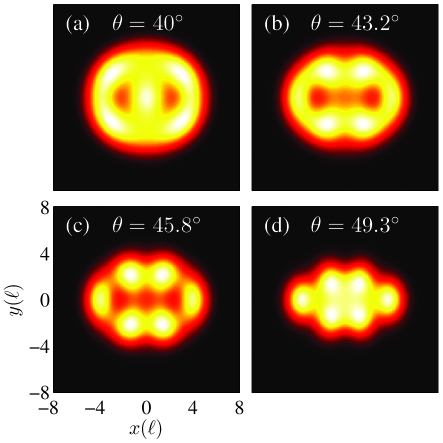
Figure 6: (Color online) Density profiles $\varrho(x,y)$ for various $\theta$s in the $N=6$ system with $\alpha=0.01$. The brightest points indicate the local maxima in the density of the system.

Table 2: Largest 5 overlaps of the anisotropic state $\left|\Psi^{(6)}(\alpha,90^{\circ})\right\rangle$ with the corresponding eigenstates in the isotropic case ($\theta=0$). The pair of ($M$, $n$) labels the $n$th lowest eigenstate in the total angular momentum $M$ subspace. The system has $n=6$ particles and $\alpha=0.01$.

$(M,n)$	$(15,0)$	$(17,0)$	$(19,2)$	$(21,7)$	$(23,14)$
${\cal O}^{(N)}_{M,n}$	0.658	0.608	0.387	0.196	0.084

In the last region $49.3^{\circ}<\theta\leq 90^{\circ}$, the most important contributions to the ground state wave function are provided by the states $\left|\Phi_{15,0}^{(6)}\right\rangle$, $\left|\Phi^{(6)}_{17,0}\right\rangle$, $\left|\Phi^{(6)}_{19,2}\right\rangle$, and $\left|\Phi^{(6)}_{21,7}\right\rangle$. The probability of finding the system in either of the above 4 states is larger than $0.92$ throughout this region. To understand the properties of the ground state in this region, we first consider the specific state at $\theta=90^{\circ}$. Table 2 lists the largest values of ${\cal O}_{M,n}^{(6)}(0.01,90^{\circ})$. Clearly, the main components of $\left|\Psi^{(6)}(0.01,90^{\circ})\right\rangle$ are the $\nu=1$ IQH state $\left|\Phi_{15,0}^{(6)}\right\rangle$ and its edge states, which suggests that, at $\theta=90^{\circ}$, the ground state is an IQH state. To confirm this, we plot the density distribution $\varrho(x,y)$ of this state in Fig. 7(a). As can be seen, the surface density for the elliptical plateau is exactly $1/2\pi\ell^{2}$, which is identical to that of a $\nu=1$ IQH state. Since the filling factor can be defined as $\nu=2\pi\ell^{2}n_{f}$ with $n_{f}$ being the fermionic surface density Lewenstein , the filling factor for the $\theta=90^{\circ}$ state is thus $1$. The homogeneous elliptical plateau of the density profile implies that our conclusion can be generalized to the thermodynamic limit. We plot the energy spectrum of the system in Fig. 7(b). It is well-known that the topological properties of the $\nu=1$ IQH state is labeled by the number of edge states, i.e., $1,1,2,3,5,\ldots$ for $\Delta L^{z}=0,1,2,3,4,\ldots$, which is exactly the case shown in Fig. 7(b), although in this case we have to replace $\Delta L^{z}$ by $\Delta\overline{M}$. All the above evidences mount to the fact that the $\theta=90^{\circ}$ state is a $\nu=1$ integer quantum Hall state. Since there is no phase transition observed in this region from various criteria, we conclude that the ground state for $\theta>49.3^{\circ}$ can be characterized as an anisotropic integer quantum Hall state.

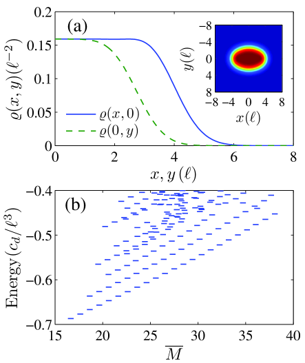
Figure 7: (Color online) Characterization of the anisotropic IQH state at $\theta=90^{\circ}$ for $N=6$ and $\alpha=0.01$. (a) The density profiles along the $x$- and $y$-axes highlight the anisotropic nature of the state. Near the center, the LLL is completely filled. The inset shows the ellipsoidal density profile on the $x$-$y$ plane. (b) The low-lying energy levels can be counted as $1$, 1, 2, 3, 5, $\ldots$ for $\Delta\overline{M}=0$, 1, 2, 3, 4, $\ldots$, respectively, which is consistent with the edge theory of an IQH state.

IV.3 Understanding the anisotropic dipolar interaction

To understand how anisotropy in the dipolar interaction leads to the emergence of the anisotropic IQH state, we decompose the dipolar interaction into isotropic and anisotropic (on $x$-$y$ plane) components as

$$V_{\theta}^{(3D)} = V_{\theta,\rm iso}^{(3D)}+V_{\theta,\rm{ani}}^{(3D)}$$ (13)

$$= \eta_{\rm iso}(\theta)\frac{r^{2}-3z^{2}}{r^{5}}+\eta_{\rm ani}(\theta)\frac{y^{2}-x^{2}}{r^{5}},$$

where $\eta_{\rm iso}(\theta)=(3\cos^{2}\theta-1)/2$ and $\eta_{\rm ani}(\theta)=3\sin^{2}\theta/2$ represent the strengths of the isotropic and anisotropic components, respectively. One should note that, to obtain Eq. (13), we have neglected the linear terms in $z$ as they vanish after we integrate out the variable $z$ to obtain the 2D interaction potential. The properties of the system can be seen as determined by the competition between $V_{\theta,\rm iso}^{(3D)}$ and $V_{\theta,\rm{ani}}^{(3D)}$. Since $\eta_{\rm iso}$ ($\eta_{\rm ani}$) is a decreasing (increasing) function of the tilt angle, varying $\theta$ will change the relative strength of the isotropic and anisotropic components, which can give rise to different quantum phases.

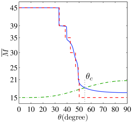
Figure 8: (Color online) Mean total angular momentum as a function of $\theta$ for $N=6$ and $\alpha=0.01$ in systems of various interactions. The solid, dashed, and dash-dotted lines correspond to, respectively, the real system with dipolar interaction, FS-I with the isotropic component only, and FS-II with the anisotropic component only. The vertical dotted line indicates the position of angle $\theta_{c}$, where the isotropic component becomes attractive.

After introducing the decomposition Eq. (13), we explore the contributions of the isotropic and anisotropic components of the dipolar interaction separately. To this end, we consider two fictitious systems, FS-I and FS-II, in which the full dipolar interaction is replaced, respectively, by $V_{\theta,\rm iso}^{(3D)}$ and $V_{\theta,\rm ani}^{(3D)}$. The corresponding Hamiltonians take the same form as Eq. (5) except for that the interaction matrix elements are replaced by those calculated using $V_{\theta,\rm iso}^{(3D)}$ or $V_{\theta,\rm ani}^{(3D)}$.

In FS-I, the strength of the isotropic interaction, $\eta_{\rm iso}(\theta)$ decreases with $\theta$. Therefore, increasing the tilt angle is effectively equivalent to increasing the strength of the confining potential $\alpha$ for the full Hamiltonian with $\theta=0$. We plot, in Fig. 8, the $\theta$ dependence of the ground state angular momentum for system-I with $N=6$ and $\alpha=0.01$. As $\theta$ is varied, FS-I experiences the same transitions as those studied in Sec. III. For the first two transitions, the critical values of $\theta$ roughly agree with those obtained using full dipolar interaction potential. In particular, $V_{\theta,{\rm iso}}^{(3D)}$ vanishes at angle $\theta_{c}=54.74^{\circ}$ and becomes attractive in the $x$-$y$ plane for $\theta>\theta_{c}$. Consequently, the ground state becomes a $\nu=1$ IQH state for $\theta\geq\theta_{c}$. The reason that the transition to the IQH state occurs at a tilt angle smaller than $\theta_{c}$ is due to the finite $\alpha$ used in Fig. 8.

In FS-II, we note that the system must be in the $\nu=1$ integer quantum state at $\theta=0$ where $V_{\theta,\rm ani}^{(3D)}$ vanishes. As one increases $\theta$, the mean total angular momentum $\overline{M}$ increases smoothly from $15$ to roughly $21$ (Fig. 8), which suggests that the system always stays in the IQH state independent of the tilt angle, although the quantum Hall droplet is stretched gradually along the $x$ axis. Further study on the ground state of FS-II can be carried out as those have been done in the previous subsection.

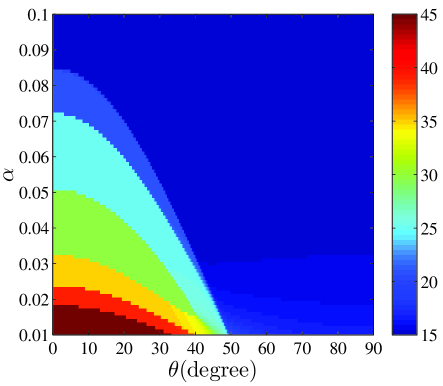
Figure 9: (Color online) Mean total angular momentum $\overline{M}(\theta,\alpha)$ of the ground state for a system with $N=6$ particles. The lower left corner is the $\nu=1/3$ Laughlin phase, while the large (blue) region containing the upper right corner is the IQH phase, which crosses over to an anisotropic IQH phase at the lower right corner.

From the above analysis, it becomes clear that the series of ground state transitions induced by varying the tilt angle are mainly caused by the isotropic component of the dipolar interaction. The anisotropic component, on the other hand, changes the fine details of the ground state, as it mixes in states with different total angular momentum to the otherwise isotropic ground state, as is clearly exemplified in the anisotropic integer quantum Hall state.

V Global phase diagram

In Secs. III and IV, we have shown the ground state transitions induced by varying either the confining strength $\alpha$ or the tilt angle $\theta$. We present the complete phase diagram in Fig. 9, in which we plot the mean total angular momentum $\overline{M}$ as a function of $\theta$ and $\alpha$ for $N=6$. The phase diagram is separated into regions with different value of $\overline{M}$, which are well defined along the $\alpha$-axis, where the interaction is isotropic, as discussed in Sec. IV. Within our numerical capabilities, we find the basic structure of Fig. 9 remains unchanged as system size $N$ varies.

We find that the Laughlin state with $\nu=1/3$ is robust for weak confinement and not too large tilt angle ($<30^{\circ}$), which assures that unintentionally introduced anisotropy in interparticle interaction is not important. On the other hand, FQH cannot survive in the large anisotropy of the dipolar interaction, when the isotropic component of the interaction becomes soft, as analyzed in Sec. IV.3.

When the confining strength becomes stronger, the mean total angular momentum $\overline{M}$ becomes smaller, indicating the system of particles becomes denser and denser. The evolution of $\overline{M}$ is not smooth, but goes through a series of magic numbers, which can be interpreted by the corresponding filling factors. In the large confinement limit, the system develops into a maximum density droplet with $\nu=1$. The state crosses over to an anisotropic maximum density droplet for large tile angles (at small confinement since the isotropic component of the interaction changes from repulsive to attractive interaction), as revealed in Fig. 7, which reflects the competition of the isotropic confining potential and both the isotropic and anisotropic components of the interaction.

VI Conclusion

To summarize, we investigated the quantum Hall effects in the LLL of a fast rotating quasi-2D Fermi gas with anisotropic dipolar interaction through exact numerical diagonalization. With the tilt angle of the dipole moment $\theta$, we introduced a new control knob to explore the FQH effect in cold atomic systems. We studied in details the phase diagram of a finite-size system and concluded that phase transition is expected as the tilt angle $\theta$ varies in the thermodynamic limit. When the tilt angle is small, the ground state of the system can be described by a FQH state, whose filling fraction depends on the strength of the confinement and hence the average density. At large tilt angle, the system eventually becomes an anisotropic $\nu=1$ IQH state. However, for intermediate $\theta$ value, we find that crystal-like order develops in the density profile of the system, suggesting the competition between various parameters and phases. By decomposing the dipolar interaction into isotropic and anisotropic components, we provide a simple explanation to quantitatively understand the phase transitions induced by anisotropy. The various competing orders and ground states are summarized in a complete phase diagram in the parameter space spanned by the tilt angle and the confinement.

In the presence of anisotropy in the interparticle interaction, we lose the rotational symmetry when treating the system in a disk geometry, hence the total angular momentum is not a good quantum number any more. Nevertheless, we demonstrated that one can still compute the expectation value of the total angular momentum operator for eigenstates and use it to characterize the various ground states emerged as the results of competitions between confinement and anisotropy, as well as between the isotropic and anisotropic components of the interparticle interaction. Particularly interesting is that the resilient features of topological order, such as the presence of hierachical FQH ground states and the low-energy excitations pertaining to the density deformation along the edge of an incompressible quantum Hall droplet, remain robust in the presence of anisotropy. While we showed that the calculation of the fidelity of the ground state can be used as a probe to detect phase transitions between states with different topological order, we believe the mean angular momentum treatment can be readily generalized to the calculation of, e.g., entanglement spectrum li08 , which also facilitates the detection of topological order.

In this paper we demonstrated that an incompressible FQH state with a large excitation gap can survive a fairly large amount of anisotropy. This implies that the Laughlin state, the exact ground state produced by the hard-core potential, is stable against the anisotropic perturbation. The finding is not unexpected given the remarkable stability of the Laughlin states in the presence of long-range interaction, finite thickness of the two-dimensional electron gas, and disorder wan05 . It is, however, intriguing to ask the effects of anisotropy on more exotic non-Abelian quantum Hall states. A more challenging question would be whether it is possible, by tuning the anisotropy, to enhance a certain FQH state, hopefully with exotic statistics. The present paper paves a path toward these questions.

References

- (1) C. Nayak, S. H. Simon, A. Stern, M. Freedman, and S. Das Sarma, Rev. Mod. Phys. 80, 1083 (2008).
- (2) W. Bishara and C. Nayak, Phys. Rev. B 80, 121302(R) (2009).
- (3) J. Xia, V. Cvicek, J. P. Eisenstein, L. N. Pfeiffer, and K. W. West, Phys. Rev. Lett. 105, 176807 (2010).
- (4) A. Wójs, C. Töke, and J. K. Jain Phys. Rev. Lett. 105, 096802 (2010).
- (5) E. H. Rezayi and S. H. Simon, Phys. Rev. Lett. 106, 116801 (2011).
- (6) I. Bloch, J. Dalibard, and W. Zwerger, Rev. Mod. Phys. 80, 885 (2008).
- (7) N. R. Cooper, Adv. Phys. 57, 539 (2008).
- (8) A. L. Fetter, Rev. Mod. Phys. 81, 647 (2009).
- (9) Y.-J. Lin, R.L. Compton, K. Jiménez-García, J.V. Porto, I.B. Spielman, Nature 462, 628 (2009).
- (10) M. Lu, S.H. Youn, and B.L. Lev, Phys. Rev. Lett. 104, 063001 (2010).
- (11) K.-K. Ni, S. Ospelkaus, M.H.G. de Miranda, A. Pe’er, B. Neyenhuis, J. J. Zirbel, S. Kotochigova, P. S. Julienne, D. S Jin, and J. Ye, Science 322, 231 (2008).
- (12) S. Ospelkaus, K.-K. Ni, M. H. G. de Miranda, B. Neyenhuis, D. Wang, S. Kotochigova, P. S. Julienne, D. S. Jin, J. Ye, Faraday Discuss. 142, 351 (2009).
- (13) K. Osterloh, N. Barberán, and M. Lewenstein, Phys. Rev. Lett. 99, 160403 (2007).
- (14) M. A. Baranov, H. Fehrmann, and M. Lewenstein, Phys. Rev. Lett. 100, 200402 (2008).
- (15) V. Fock, Zeitschrift fär, Physik 47, 446 (1928).
- (16) C. G. Darwin, Proc. Cambridge Phil. Soc. 27, 86 (1930).
- (17) R. B. Laughlin, Phys. Rev. Lett. 50, 1395 (1983).
- (18) S. M. Girvin and T. Jach, Phys. Rev. B 28, 4506 (1983).
- (19) J. K. Jain, Phys. Rev. Lett. 63, 199 (1989).
- (20) J. K. Jain and T. Kawamura, Europhys. Lett. 29, 321 (1995).
- (21) T. Seki, Y. Kuramoto, and T. Nishino, J. Phys. Soc. Jpn. 65, 3945 (1996).
- (22) P. A. Maksym, Phys. Rev. B 53, 10871 (1996).
- (23) C. Yannouleas and U. Landman, Phys. Rev. B 68, 035326 (2003).
- (24) R. B. Laughlin, Phys. Rev. B. 27, 3383 (1983).
- (25) X.-G. Wen, Quantum Field Theory of Many-Body Systems, (Oxford University Press, 2004).
- (26) H. T. Quan, Z. Song, X. F. Liu, P. Zanardi, and C. P. Sun, Phys. Rev. Lett. 96, 140604 (2006).
- (27) See, e.g., S. J. Gu, Int. J. Mod. Phys. B 24, 4371 (2010).
- (28) H. Li and F. D. M. Haldane, Phys. Rev. Lett. 101, 010504 (2008).
- (29) X. Wan, D. N. Sheng, E. H. Rezayi, K. Yang, R. N. Bhatt, and F. D. M. Haldane, Phys. Rev. B 72, 075325 (2005).