Monte Carlo generator ELRADGEN 2.0 for simulation of radiative events in elastic $ep$-scattering of polarized particles

Abstract

The structure and algorithms of the Monte-Carlo generator ELRADGEN 2.0 designed to simulate radiative events in polarized $ep$-scattering are presented. The full set of analytical expressions for the QED radiative corrections is presented and discussed in detail. Algorithmic improvements implemented to provide faster simulation of hard real photon events are described. Numerical tests show high quality of generation of photonic variables and radiatively corrected cross section. The comparison of the elastic radiative tail simulated within the kinematical conditions of the BLAST experiment at MIT BATES shows a good agreement with experimental data.

PROGRAM SUMMARY

Manuscript title: Monte Carlo generator ELRADGEN 2.0 for simulation of radiative events in elastic $ep$-scattering of polarized particles
Authors: I. Akushevich, O.F. Filoti, A. Ilyichev, N. Shumeiko
Program title: ELRADGEN 2.0
Licensing provisions: none
Programming language: FORTRAN 77
Computer(s) for which the program has been designed: all
Operating system(s) for which the program has been designed: any
RAM required to execute with typical data: 1 MB
Has the code been vectorised or parallelized?: no
Number of processors used: 1
Supplementary material: none
Keywords: radiative corrections, Monte Carlo method, elastic $ep$-scattering
PACS: 07.05.Tp, 13.40.Ks, 13.88.+e, 25.30.Bf
CPC Library Classification:
External routines/libraries used: none
CPC Program Library subprograms used: none

Nature of problem: simulation of radiative events in polarized $ep$-scattering.
Solution method: Monte Carlo simulation according to the distributions of the real photon kinematic variables that are calculated by the covariant method of QED radiative correction estimation. The approach provides rather fast and accurate generation.
Restrictions: none
Unusual features: none
Additional comments: none
Running time: the simulation of $10^{8}$ radiative events for $itest:=1$ takes up to 3 minutes 9 seconds on Pentium(R) Dual-Core 2.00 GHz processor.

1 Introduction

The exclusive photon production in lepton-nucleon scattering is the routine experimental tool in investigating the hadronic structure. Depending on the design of experiments, the measurements of this process can give an access to the generalized parton distributions [1, 2] or the generalized polarizabilities [3, 4]. In some cases the exclusive photon production appears as a background effect to inelastic [5, 6] or elastic [7] lepton nucleon scattering. The last scenario, i.e. the situation when the events with the real photon emission accompany the elastic electron-proton scattering is the most advanced due to the infrared problem, therefore it will be in our main focus.

The set of processes contributed to the observed cross section in the next order of perturbation theory is referred to as the lowest order radiative corrections (RC). The basic contribution to the lowest order RC appears from the square of amplitude that only includes real photon emission from the lepton leg. This contribution contains the so-called large logarithm (i.e., the logarithm of the lepton mass) and normally is only held in the lowest order RC.

In practice of data analysis, RC are calculated theoretically or their contribution to the observed cross sections (or asymmetries) are minimized by experimental methods. Due to finite detector resolution, a complete removal of the events with radiated hard photon(s) by pure experimental methods is not possible. Furthermore, the contributions of additional virtual particles and soft photon emission cannot be removed in principle. The theoretical calculation provides with analytical expressions included the contributions of loops and photon emission which are infrared free after the procedure of the cancellation of the infrared divergence. The contribution of the hard photon radiation is presented in the form of integrals over photon phase space. Partly the integration is performed analytically without additional simplifying assumptions or assumptions on specific functional forms describing hadronic structure.

The pioneering approach for RC calculation in inelastic processes was suggested by Mo and Tsai in their seminal paper in 1969 [8]. They also developed the peaking approximation allowing for analytical estimating integrals over photon angles. The approximation is used in many data analysis, e.g. , in ref. [9] the electromagnetic RC in elastic $ep$-scattering was calculated in peaking approximation with taking into account the one-photon emission both from lepton and hadron legs.

The Mo and Tsai approach requires involvement of the artificial parameter $\Delta$ separating the integration region over photon energy on parts with soft and hard photon contributions. To cancel infrared divergence analytically only leading terms in the expansion of the soft photon contribution over reciprocal of the photon energy are kept. As a result, the final expressions contain undesired dependence on the artificial parameter.

Bardin and Shumeiko developed the approach [10] for exact separation and cancellation of infrared divergence when the final expressions for RC were completely free from any artificial parameters like $\Delta$. Using this approach, RC in polarized elastic $ep$-scattering withing QED theory has been calculated in refs. [11, 12]. Basing on these calculations the FORTRAN code MASCARAD has been developed and successfully used for data processing of the relevant parity conservation experiments [13, 14]. Other approaches were also used for RC calculation in elastic $ep$-scattering. Thus, the total lowest order RC (both to lepton and hadron legs) was also calculated in [7] with soft photon approximation and the method of electron structure functions suggested in the work [15] was also applied for estimation of RC to elastic $ep$ scattering [16, 17].

The use of realistic detector geometry requires essentially complicated integration over the real photon phase space. As a result, the researchers come to the necessity of using the Monte Carlo technique which constitutes a complementary approach to the theoretical calculations of RC using respective codes such as MASCARAD. The Monte Carlo generators for simulation of radiative events have been developed for many specific processes and intensively used in data analysis. Thus, the Monte Carlo generator RADGEN [18] for simulation of radiative events in inclusive deep inelastic scattering has been developed on the basis of the FORTRAN code POLRAD [19]. The Monte Carlo generator MERADGEN [20] for simulation of radiative events in Møller scattering appeared on the base of FORTRAN code MERA [21].

In this paper we present and describe in detail the latest version 2.0 of the Monte Carlo generator ELRADGEN. The prototype of the code [22] dealt with the simulation of real hard photon emission as a background effect in the unpolarized elastic electron-proton scattering. The present version 2.0 is extended on the initial polarized particles: longitudinally polarized electron and arbitrary polarized proton. The theoretical background for the developments is presented in ref. [11].

The paper is organized as follows. Section 2 describes the kinematics of the investigated process and the generation method. The different contributions to the lowest order RC and the multi-soft photon emission are presented and discussed in Section 3. The brief structure of the code and the input-output datafiles are described in Section 4. Test runs, comparison with MASCARAD, and numerical comparison of the simulated and measured cross sections of the radiative tail from elastic peak in the BLAST experiment are presented in Section 5. Conclusions and final remarks are given in Section 6. The four-momenta reconstruction formulae, explicit expressions for the lepton and target polarization vectors, some lengthy formulae for RC, and test outputs are given in Appendices.

Figure 1: Feynman graphs contributing to radiatively corrected cross sections of elastic lepton-nucleus scattering: Born (a), additional virtual particles (b,c) and real photon emission (d,e) contributions.

2 Kinematics and Method of Generation

The lowest order (Born) (Fig.1 (a)) as well as the additional virtual particle (Fig.1 (b,c)) contributions to the polarized elastic lepton-nucleon scattering

$$e(k_{1},\;\xi_{L})+p(p_{1},\;\eta)\longrightarrow e^{\prime}(k_{2})+p^{\prime}(p_{2})$$ (1)

($k_{1}^{2}=k_{2}^{2}=m^{2}$, $p_{1}^{2}=p_{2}^{2}=M^{2}$) can be described by the following three variables:

$$Q^{2}=-q^{2}=-(k_{1}-k_{2})^{2},\qquad S=2k_{1}p_{1},\quad\phi,$$ (2)

where $\phi$ is the azimuthal angle between the scattering plane ${\bf(k_{1},k_{2})}$ and the ground level. The Lab system is used with OZ axis along the beam direction and plane OZX parallel to the ground level. The explicit expressions of polarization vectors ($\xi_{L}$ and $\eta$) and four-momenta reconstructed in the lab system are presented in Appendix A.

The description of the phase space of the radiative process (Fig.1(d,e))

$$e(k_{1},\;\xi_{L})+p(p_{1},\;\eta)\longrightarrow e^{\prime}(k_{2})+p^{\prime}(p_{2})+\gamma(k),$$ (3)

($k^{2}=0$) requires three new kinematic variables: a virtual proton transfer momentum squared $t=-(k_{1}-k_{2}-k)^{2}$, the inelasticity $v=(p_{2}+k)^{2}-M^{2}$, and the azimuthal angle $\phi_{k}$ between the planes ${\bf(q,k)}$ and ${\bf(k_{1},k_{2})}$. This set of variables defines the four-momenta of all final particles.

The simulation of radiative events requires an additional definition of the lowest bound of the photon energy (or another respective quantity, inelasticity $v_{min}$ in our case) separating the photon phase space into the region of soft and hard photons. Only hard photons need to be simulated while soft photons cannot be simulated because of the infrared divergence. The observed cross section can be presented in terms of two positively definite parts:

$$\sigma_{obs}=\sigma_{rad}(v_{min})+\sigma_{BSV}(v_{min}).$$ (4)

The first term, $\sigma_{rad}(v_{min})$, describes the cross section with an additional hard photon emitted, and the second, $\sigma_{BSV}(v_{min})$, contains the contributions of the Born cross section, soft-photon emission, and virtual corrections. Here and later we define $\sigma\equiv d\sigma/dQ^{2}d\phi$. Note that $\sigma_{obs}$ does not depend on $v_{min}$ while terms $\sigma_{BSV}$ and $\sigma_{rad}$ do.

The strategy for simulation of one event can be defined in a standard way [22]:

• For the fixed initial energy, $Q^{2}$, the angle $\phi$, and the missing mass square resolution $v_{min}$, the two positively-definite contributions to the observed (radiative-corrected) cross section $\sigma_{obs}$, $\sigma_{rad}(v_{min})$, and $\sigma_{BSV}(v_{min})$ are calculated separately.

• The corresponding channel of scattering (i.e., BSV or radiative process) is simulated for this event in accordance with partial contributions of these two positive parts into the total cross section. More specifically, the channel of scattering is simulated in accordance with the Bernoulli trial where the probability of “success” (i.e., radiative channel) is calculated as a ratio of the radiative part of the cross section to the total cross section.

• For the radiative event the kinematic variables $t$, $v$ and $\phi_{k}$ are simulated in accordance with their calculated distributions. The distributions of $v$ and $\phi_{k}$ are conditional (e.g. , $v$ is simulated conditionally on $t$, and $\phi_{k}$ is simulated conditionally on $t$ and $v$). The explicit expressions for the probability densities of these variables are defined by eqs. 15.

• The four–momenta of all final particles in a required reference frame are calculated.

The initial values of $Q^{2}$ (and $\phi$) can be non-fixed but externally simulated according to a probability distribution (for example, the Born cross section). If the $Q^{2}$ distribution is simulated over the Born cross section, then the realistic observed $Q^{2}$ distribution is calculated as sum of weights computed as ratios of the total and Born cross sections for each simulated event. If the observed cross section is used for the simulation of $Q^{2}$, then reweighting is not required.

3 Explicit expressions for $\sigma_{rad}(v_{min})$ and $\sigma_{BSV}(v_{min})$

The analytical expressions for the lowest order RC on which the ELRADGEN is based, were obtained in ref. [11] (see eqs. (50) and (51)). The result for the observed cross section can be formally outlined as $\displaystyle\sigma_{obs}=(1+\delta)\sigma_{0}+C\int\frac{dv}{v}[\sigma_{R}(v)-\sigma_{0}]$, where $C$ is a kinematic coefficient proportional to $\alpha$ and the quantity $\sigma_{R}(v)$ is proportional to the bremsstrahlung cross section ($\sigma_{R}(0)=\sigma_{0}$). This expression does not reproduce the form of eq. (4), because the term with the integral is not positively definite and the term with $\sigma_{R}(v)$ cannot be separated because it is singular for $v\rightarrow 0$. Instead, the following transformation of this term was used:

$$\int{dv\over v}(\sigma_{R}(v)-\sigma_{0})=\int{dv\over v}\sigma_{R}(v)\theta(v-v_{min})$$

$$\qquad\qquad-\int{dv\over v}\sigma_{0}\theta(v-v_{min})+\int{dv\over v}[\sigma_{R}(v)-\sigma_{0}]\theta(v_{min}-v).$$ (5)

The first term in (5) represents the contribution of hard photons, i.e., with inelasticity above $v_{min}$. This term is positively definite and it is used as $\sigma_{rad}(v_{min})$ in (4). Its structure and explicit expressions are discussed in Section 3.2. The second term admits the analytic integration resulting in correction $\delta^{add}(v_{min})$. This term (as well as the third term in the eq. (5) discussed in Section 3.3) contributes to the $\sigma_{BSV}(v_{min})$ that represents the part of the observed cross section not contained in the contributions of radiated photons with inelasticity above $v_{min}$.

3.1 $BSV$ cross section

The $BSV$-part of observed cross section includes the Born cross section (Fig.1 (a)), loop effects (Fig.1 (b,c)) and the contribution of soft photons. The latter is restricted by the inelasticity value $v<v_{min}$:

$$\sigma_{BSV}(v_{min}) = (1+\delta_{VR}+\delta_{vac}^{l}+\delta_{vac}^{h})e^{\delta_{inf}}\sigma_{0}+\delta^{add}(v_{min})\sigma_{0}$$ (6)

$$+\sigma^{add}_{R}(v_{min}).$$

The Born contribution to the cross section reads:

$$\sigma_{0}=\frac{\alpha^{2}}{S^{2}Q^{4}}\sum_{i=1}^{4}\theta_{i}^{B}{\mathcal{F}}_{i}(Q^{2}).$$ (7)

The kinematic coefficients $\theta_{B}$ are presented in Appendix B. The structure functions ${\mathcal{F}}_{i}$ are the squared combinations of the electric and magnetic elastic form factors:

$${\mathcal{F}}_{1}(Q^{2})=4\tau_{p}M^{2}G_{M}^{2}(Q^{2}),\;\;{\mathcal{F}}_{2}(Q^{2})=4M^{2}\frac{G_{E}^{2}(Q^{2})+\tau_{p}G_{M}^{2}(Q^{2})}{1+\tau_{p}},$$

$${\mathcal{F}}_{3}(Q^{2})=-2M^{2}G_{E}(Q^{2})G_{M}(Q^{2}),\;\;$$

$${\mathcal{F}}_{4}(Q^{2})=-M^{2}G_{M}(Q^{2})\frac{G_{E}(Q^{2})-G_{M}(Q^{2})}{1+\tau_{p}}$$ (8)

with $\tau_{p}=Q^{2}/4M^{2}$.

The factorizing corrections in the first term of (6) describe the effects of loops and soft-photon emission. The correction $\delta_{inf}$ comes from the emission of soft photons, the $\delta_{VR}$ appears as a result of an infrared cancellation of real (Fig.1 (d,e)) and virtual (Fig.1 (c)) photon contribution. The explicit expressions for them are:

$$\delta_{inf} = {\alpha\over\pi}\Bigl{(}\log\frac{Q^{2}}{m^{2}}-1\Bigr{)}\log\frac{v_{max}^{2}}{S(S-Q^{2})},$$

$$\delta_{VR} = {\alpha\over\pi}\biggl{(}\frac{3}{2}\log\frac{Q^{2}}{m^{2}}-2-\frac{1}{2}\log^{2}\frac{S}{S-Q^{2}}+{\rm Li}_{2}\biggl{(}1-\frac{M^{2}Q^{2}}{S(S-Q^{2})}\biggr{)}$$ (9)

$$-\frac{\pi^{2}}{6}\biggr{)},$$

where ${\rm Li}_{2}$ is the Spence function.

The effect of vacuum polarization by leptons (hadrons) depicted on Fig.1 (b) is described by $\delta^{l}_{vac}$ ($\delta^{h}_{vac}$). The explicit expression for $\delta^{l}_{vac}$ is defined by eq. (21) of ref. [5] while the fit for $\delta^{h}_{vac}$ has been taken from [23].

The term $\delta^{add}(v_{min})\sigma_{0}$ in the R.H.S. of (6) contains the correction coming from the second term in (5).

$$\delta^{add}(v_{min}) = -\frac{2\alpha}{\pi}\Bigl{(}\log\frac{Q^{2}}{m^{2}}-1\Bigr{)}\log\frac{v_{max}}{v_{min}}.$$ (10)

The last term in (6) is discussed in Section 3.3.

3.2 Bremsstrahlung cross section

\begin{picture}(160.0,80.0)\put(20.0,0.0){ \epsfbox{figures/vt.eps} } \end{picture}

Figure 2: The region of integration over $v$- and $t$-variables for JLab kinematics ($Q^{2}=3$ GeV², $S=7.5$ GeV²). The line $v=v_{min}$ splits it into hard (solid lines) and soft (dashed lines) real photon regions.

Since the structure functions depend only on $t$, and therefore integrals over other variables (i.e., $v$ and $\phi_{k}$) can be evaluated analytically or numerically with high precision, a reasonable sequence of integration variables is chosen such that integration over $t$ is external. This approach allows us to speed up the generation of radiative events. The radiative photon phase space for $t$- and $v$-variables are presented on Fig. 2. It is separated into hard and soft photon emission by the line $v=v_{min}$. The cross section of hard-photon bremsstrahlung is

$$\sigma^{rad}(v_{min})=-{\alpha^{3}\over 4\pi S^{2}}\int\limits_{t_{1}}^{t_{2}}dt\sum_{i=1}^{4}{{\mathcal{F}}_{i}(t)\over t^{2}}\theta_{i}^{R}(v_{1},v_{max}).$$ (11)

The quantities $\theta_{i}^{R}(v_{1},v_{max})$ result from the integration over inelasticity $v$. Their arguments correspond to the limits of integration:

$$\theta_{i}^{R}(v_{1},v_{max}) = \sum_{j=1}^{k_{i}}\int\limits_{v_{1}}^{v_{max}}dvR^{j-3}\theta_{ij}^{R}(v).$$ (12)

Here $R=Q^{2}+v-t$, and the upper sum limits are defined as $k_{i}=(3,3,4,5)$. Accordingly, the quantities $\theta_{ij}^{R}(v)$ result from the integration over $\phi_{k}$:

$$\theta_{ij}^{R}(v) = \int\limits_{0}^{2\pi}d\phi_{k}\ \theta_{ij}^{R}(v,\phi_{k}).$$ (13)

The set of quantities $\theta^{R}$ is defined in Appendix B.

Kinematical bounds are defined as

$$v_{1} = \max\{\frac{(t-Q^{2})(\sqrt{t}-\sqrt{4M^{2}+t})}{2\sqrt{t}},\frac{(t-Q^{2})(\sqrt{t}+\sqrt{4M^{2}+t})}{2\sqrt{t}},$$

$$\qquad v_{min}\},\;$$

$$v_{max} = \frac{2Q^{2}(S^{2}-4M^{2}m^{2}-Q^{2}(S+m^{2}+M^{2}))}{Q^{2}(S+2m^{2})+\sqrt{Q^{2}(S^{2}-4M^{2}m^{2})(Q^{2}+4m^{2})}}$$

$$\approx S-Q^{2}-\frac{M^{2}Q^{2}}{S},$$

$$t_{1,2} = \frac{2M^{2}Q^{2}+v_{max}\left(Q^{2}+v_{max}\mp\sqrt{(Q^{2}+v_{max})^{2}+4M^{2}Q^{2}}\right)}{2(M^{2}+v_{max})}.$$ (14)

The probability distributions used for simulation of the photonic variables are obtained using (11) and (13):

$$\rho(t) = \frac{1}{N_{t}}\sum_{i=1}^{4}\frac{{\mathcal{F}}_{i}(t)}{t^{2}}\theta_{i}^{R}(v_{1},v_{max}),\;\;\;\;N_{t}=\sum_{i=1}^{4}\int\limits_{t_{1}}^{t_{2}}dt\frac{{\mathcal{F}}_{i}(t)}{t^{2}}\theta_{i}^{R}(v_{1},v_{max}),$$

$$\rho(v|t) = \frac{1}{N_{v}}\sum_{i=1}^{4}\sum_{j=1}^{k_{j}}{\mathcal{F}}_{i}(t)\theta_{ij}^{R}(v)R^{j-3},\;\;N_{v}=\sum_{i=1}^{4}{\mathcal{F}}_{i}(t)\theta_{i}^{R}(v_{1},v_{max}),\qquad$$

$$\rho(\phi_{k}|v,t) = \sum_{i=1}^{4}\sum_{j=1}^{k_{j}}\frac{\displaystyle{\mathcal{F}}_{i}(t)\theta_{ij}^{R}(v,\phi_{k})R^{j-3}}{N_{\phi_{k}}},\;N_{\phi_{k}}=\sum_{i=1}^{4}\sum_{j=1}^{k_{j}}{\mathcal{F}}_{i}(t)\theta_{i}^{R}(v)R^{j-3}.\;\;$$ (15)

3.3 Contribution of $\sigma_{R}^{add}(v_{min})$

The contribution of $\sigma_{R}^{add}(v_{min})$ can be presented as an integral over the soft-photon region in Fig. 2:

$$\sigma_{R}^{add}{(v_{min})} = -{\alpha^{3}\over 4\pi S^{2}}\int\limits_{t^{\prime}_{1}}^{t^{\prime}_{2}}dt\int\limits_{v^{\prime}_{1}}^{v_{min}}dv\sum_{i=1}^{4}\Biggl{[}\sum_{j=2}^{k_{j}}R^{j-3}\theta_{ij}^{R}(v){{\mathcal{F}}_{i}(t)\over t^{2}}$$ (16)

$$+\frac{1}{R^{2}}\Biggl{(}\theta_{i1}^{R}(v){{\mathcal{F}}_{i}(t)\over t^{2}}-4\theta^{B}_{i}F_{IR}(v){{\mathcal{F}}_{i}(Q^{2})\over Q^{4}}\Biggr{)}\Biggr{]}.$$

The limits of integration over variables $t$ and $v$ read:

$$v_{1}^{\prime} = \max\{\frac{(t-Q^{2})(\sqrt{t}-\sqrt{4M^{2}+t})}{2\sqrt{t}},\;\frac{(t-Q^{2})(\sqrt{t}+\sqrt{4M^{2}+t})}{2\sqrt{t}}\},\;$$

$$t_{1,2}^{\prime} = \frac{2M^{2}Q^{2}+v_{min}\left(Q^{2}+v_{min}\mp\sqrt{(Q^{2}+v_{min})^{2}+4M^{2}Q^{2}}\right)}{2(M^{2}+v_{min})}.$$ (17)

The infrared divergences could occur in the limit $v_{1}^{\prime}\to 0$ (i.e. at $t\to Q^{2}$) in the terms containing $R^{-2}$. However, one can see that $\sigma_{R}^{add}{(v_{min})}$ is infrared-free. Indeed, taking into account Eqs. (13), (B.12), (B.15), and (B.16), in the limit $v_{1}^{\prime}\to 0$ we have

$$\lim_{v\to 0}\theta_{i1}^{R}(v){{\mathcal{F}}_{i}(t)\over t^{2}}=4\theta^{B}_{i}F_{IR}(0){{\mathcal{F}}_{i}(Q^{2})\over Q^{4}}.$$ (18)

This cancels one degree of $R$. The second degree of $R$ cancels because the integration region is collapsed into a point within this limit.

4 The structure of the program and input-output data

Figure 3: The structure of the program ELRADGEN 2.0

4.1 The structure of the program

The set of files included in the package ELRADGEN 2.0 contains three FORTRAN files (elradgen.f, run.f, test.f), six INCLUDE files (const.inc, grid.inc, output.inc, par.inc, pol.inc, test.inc), two data files (rnd.dat, test.dat), and one Makefile. No installation is required for this code.

The elradgen.f is a source code of the Monte Carlo generator ELRADGEN 2.0. It contains the set of functions and subroutines for simulation of a single event. The loop over simulated events as well as initialization of constants requires coding in the external program. Two versions of such external programs are given in files run.f and test.f. The file run.f is a typical external program for simulation of an event with fixed $Q^{2}$ and $\phi$. The file test.f is designed to run several tests discussed below.

The structure of the code is illustrated in Fig. 3:

• program main is a sample of an external program that invokes ELRADGEN (in our case it is the program included in run.f and test.f);

• elrad$\_$init defines all constants (such as beam energy and polarization degrees) which are necessary for generation;

• grid$\_$init prepares the grids for generation of photonic kinematic variables;

• elradgen is a main subroutine governing the simulation of an event;

• urand is a generator of uniformly distributed random numbers;

• fsib calculates the Born cross section;

• fsigt invokes one of the subroutines fsigtan or fsigtnu to calculate the cross section $d\sigma/dt$;

• fsigtan calculates the analytical cross section $d\sigma/dt$ for unpolarized scattering;

• fsigtnu calculates the cross section $d\sigma/dt$ with numerical integration over variable $v$ for polarized scattering;

• fsigtv calculates the analytical cross sections $d\sigma/(dtdv)$ and $d\sigma/(dtdvd\phi_{k})$;

• ffpro is a model for elastic form factors.

The six INCLUDE files are:

• const.inc includes all necessary constants, e.g. , the fine electromagnetic constant, the proton and lepton masses;

• grid.inc includes nets of bins for simulation of the three photonic variables;

• output.inc contains variables governing the form of output as discussed below

• pol.inc includes quantities which describe the polarization state (defined in Appendix A.1);

• test.inc includes variables and nets of bins required for test run;

• par.inc includes variables required for calculation of $\sigma^{add}_{R}(v_{min})$.

The file rnd.dat includes an initial integer for the flat generator urand, and test.dat is an example of output data for a test run (when test.f is used as an external program); the results of different test are presented in Appendix C.

The commands “make” or “make test” need to be run for creating the executable file for the simulation or for the test runs, respectively.

4.2 Input-output data

Input data in ELRADGEN 2.0 are set up in program main of run.f or test.f. Majority of them are transferred to the main program through parameters in the subroutine elradgen. They are:

• ebeam is an energy of electron beam;

• q2 is a virtual photon momentum squared $Q^{2}$;

• phi is an azimuthal angle between the scattering plane and the ground level;

• vvmin is a missing mass square resolution $v_{min}$ for separation of radiatively corrected cross section into radiative and BSV parts;

• vcut is a cut-off quantity $v_{cut}$ that allows to exclude the simulation of hard photons above $v_{cut}$.

The last variable provides the opportunity to exclude simulation of events with inelasticity above a predetermined level. This could be convenient when simulation is performed for experimental design, when hard real photon are removed from experimental data by putting a cut on the missing mass of the undetectable particle.

The quantities describing the polarization characteristics of beam and target (defined in Appendix A.1) are transferred to the code through the common block pol containing four variables: i,ii) $plrun$ and $pnrun$, the polarization degrees of the lepton beam $P_{L}$ and target $P_{N}$, iii) $thetapn$, the angle $\theta_{\eta}$ between 3-vectors of the target polarization $\boldsymbol{\eta}$ and initial lepton momentum $\bf k_{1}$, and iv) $phipn$, the angle $\phi_{\eta}$ between OZX and ($\bf k_{1}$, $\boldsymbol{\eta}$) planes.

One additional variable $itest$ governs the form of the output. If $itest\neq 0$, all output information is printed to the file test.dat. If $itest=0$, the output data are collected in two common blocks of the file output.inc:

common/variables/tgen,vgen,phigen,weight,ich

and

common/vectors/vprad,phrad

Here $tgen$, $vgen$, and $phigen$ are the generated photonic variables $t$, $v$, and $\phi_{k}$, respectively, $weight$ is a ratio of the observable cross section to the Born one, variable $ich$ shows whether the scattering channel is radiative ($ich=1$) or BSV ($ich=0$). The quantities $vprad=p_{2}-p_{1}$ and $phrad:=k$ are four-momenta of virtual and real photons defined in the Lab system.

For BSV events, $vgen=0$, $tgen=Q^{2}$, $\phi_{k}=0$, $phrad=0$ and $vprad=k_{1}-k_{2}$.

5 Numerical tests and comparison with experimental data

Below we describe three types of numerical experiments allowing: i) to crosscheck some key distributions and parameter estimates in ELRADGEN, ii) to investigate issues related to a possible dependence of simulated cross sections on $v_{min}$, and iii) to perform a comparison with data collected in the BLAST experiment.

5.1 Tests implemented in ELRADGEN

There are five tests implemented in the program. The first three deal with checking to which extent the simulated distributions on photonic variables $t$, $v$, and $\phi_{k}$ correspond to analytical probability distributions given in eq. (15).

\begin{picture}(80.0,80.0)\put(-5.0,0.0){ \epsfbox{figures/tgent.eps} } \end{picture}
\begin{picture}(80.0,80.0)\put(-5.0,0.0){ \epsfbox{figures/phigent.eps} } \end{picture}

Figure 4: Histogram (points) and corresponding probability densities (solid lines) for variables describing the exclusive real hard photon production in polarized electron proton scattering at JLab kinematic conditions ($E_{beam}=4$ GeV, $Q^{2}=3$ GeV², ) for transverse polarized proton ($\theta_{\eta}=90^{0}$) with $\phi=\phi_{\eta}$, $P_{L}P_{N}=-1$ and $v_{min}=10^{-2}$ GeV².

Fig. 4 presents the $t$-, $v$-, and $\phi_{k}$-distributions calculated numerically and generated by ELRADGEN under JLab kinematic conditions for a transverse polarized target. The theoretical and simulated distributions of this case (as well as for unpolarized and longitudinally polarized targets) are almost identical.

The sharp peaks in the $t$-distribution coming from the collinear singularities, i.e., from the kinematical region where the real photon is emitted along either the initial or the final lepton. After integration over the inelasticity $v$, these two singularities are situated near $t=Q^{2}$ and are only slightly different.

The peaks on the plots of the $v$-distributions correspond to the collinear singularities as well. Since the variable $t$ is external, the $v$-distribution is conditional on $t$, and therefore only one peak corresponding to either the initial or the final electron appears for each $v$-distribution.

Finally, the $\phi_{k}$-distributions show that most of the photons are emitted in the scattering plane.

For generation of the three types of distributions, one has to set $itest=1$, $itest=2$, or $itest=3$, in the file test.f, and then type ”make test” and ”./test.exe”. In Appendix C, the test outputs for $t$, $v$, and $\phi_{k}$ generation with $P=1$, $E_{b}^{\rm Lab}$=4 GeV, $\theta_{\eta}=48^{0}$, 20 bins for the histogramming and $10^{8}$ radiative events are presented.

After generating all photonic variables for one radiative event, ELRADGEN reconstructs the four-momenta of the final particles. To make sure that the vectors are constructed properly, the next test corresponding to $itest:=4$ is implemented. This test allows to perform the numerical comparison of the generated variables $t$, $v$, and $\phi_{k}$ with the value of these variables reconstructed from four-momenta of the particles. This test also reconstructs the mass of the real photon that has to be equal to zero.

The test with $itest:=5$ provides us with the comparison of the unpolarized cross section integrated over $v$ analytically and numerically.

5.2 $v_{min}$-dependence and comparison with MASCARAD

The Monte Carlo generator ELRADGEN 2.0 was developed on the basis of the FORTRAN code MASCARAD, therefore the agreement of outputs of both programs with the same input parameters has to be demonstrated as a primary test. Here we restrict our crosscheck to the JLab kinematic conditions without cuts on inelasticity $v$ and focus on the comparison of the ratio of the radiatively corrected cross section to the Born one. Define components of the cross sections as:

$$\sigma^{L,T}_{a}(\xi_{L},\eta_{L,T})=\sigma^{u}_{a}+P_{L}P_{N}\sigma^{p}_{a}(\xi_{L},\eta_{L,T}),$$ (19)

where $a=0,BSV,rad,obs$

$v_{min}$	$\sigma^{u}_{rad}/\sigma^{u}_{0}$		$\sigma^{u}_{BSV}/\sigma^{u}_{0}$		$weight=\sigma^{u}_{obs}/\sigma^{u}_{0}$
GeV2	a	b	a	b	a	b	c
1	1.144	1.145	0.9730	0.9737	2.117	2.119
$10^{-1}$	1.316	1.317	0.8018	0.8018	2.118	2.118
$10^{-2}$	1.478	1.473	0.6386	0.6386	2.116	2.111	2.117
$10^{-3}$	1.641	1.634	0.4754	0.4754	2.116	2.108
$10^{-4}$	1.806	1.797	0.3122	0.3122	2.118	2.108

Table 1: The $v_{min}$-dependence of the ratios of radiative, BSV, and observable contributions to the unpolarized ($P_{L}P_{N}\equiv 0$) electron-proton cross section to the Born cross section for JLab kinematic conditions ($E_{beam}=4$ GeV and $Q^{2}=3$ GeV²): a (b) presents the results of analytical (numerical) integration over $v$ in ELRADGEN, while c shows the results of the calculation using MASCARAD [11].

$v_{min}$	$\sigma^{L}_{rad}/\sigma^{L}_{0}$		$\sigma^{L}_{BSV}/\sigma^{L}_{0}$		$weight=\sigma^{L}_{obs}/\sigma^{L}_{0}$
GeV2	ELRADGEN		ELRADGEN		ELRADGEN		MASCARAD
$P_{L}P_{N}$	1	-1	1	-1	1	-1	1	-1
1	0.6277	1.275	0.9648	0.9765	1.592	2.251
$10^{-1}$	0.7913	1.448	0.8009	0.8080	1.592	2.250
$10^{-2}$	0.9469	1.605	0.6385	0.6487	1.585	2.243	1.591	2.249
$10^{-3}$	1.106	1.764	0.4754	0.4893	1.582	2.240
$10^{-4}$	1.269	1.927	0.3122	0.3300	1.582	2.240

Table 2: $v_{min}$-dependence of the radiative, BSV, and observable contribution to electron-proton scattering with longitudinally polarized target ($\theta_{\eta}=0$) for a different spin orientation in the Born units and comparison with MASCARAD [11] for JLab kinematic conditions ($E_{beam}=4$ GeV and $Q^{2}=3$ GeV²).

$v_{min}$	$\sigma^{T}_{rad}/\sigma^{T}_{0}$		$\sigma^{T}_{BSV}/\sigma^{T}_{0}$		$weight=\sigma^{L}_{obs}/\sigma^{T}_{0}$
GeV2	ELRADGEN		ELRADGEN		ELRADGEN		MASCARAD
$P_{L}P_{N}$	1	-1	1	-1	1	-1	1	-1
1	0.9457	1.447	0.9730	0.9746	1.919	2.422
$10^{-1}$	1.117	1.620	0.8018	0.8018	1.918	2.422
$10^{-2}$	1.273	1.776	0.6386	0.6386	1.912	2.415	1.917	2.420
$10^{-3}$	1.432	1.935	0.4754	0.4754	1.908	2.411
$10^{-4}$	1.596	2.099	0.3122	0.3122	1.908	2.411

Table 3: $v_{min}$-dependence of the radiative, BSV and observable contribution to electron-proton scattering with transversely polarized target ($\theta_{\eta}=\pi/2$, $\phi=\phi_{\eta}$) for different spin orientation in the Born units and comparison with MASCARAD [11] for JLab kinematic conditions ($E_{beam}=4$ GeV and $Q^{2}=3$ GeV²).

First, we consider the unpolarized scattering for which an option with analytical integration over $v$ is available. Table 1 presents the results of the analytical and numerical integration for the BVS- and radiative contributions (i.e., $\sigma_{BSV}(v_{min})$ and $\sigma_{rad}(v_{min})$) to the observed cross section, as well as the results obtained using MASCARAD. Each of these contributions changes essentially by decreasing $v_{min}$ from 1 to $10^{-4}$ GeV², while the observable cross sections barely change for both analytical and numerical integration over $v$. The similar behavior of the radiative and BSV parts takes place for the polarized case. This is illustrated in Tables 2 and 3. The observable cross sections change by no more than 1%.

5.3 Results from the BLAST data

Analyzing the $\Delta$-excitation region in $ep$-scattering, it is necessary to extract the contribution of real hard-photon emission that accompanies the elastic $ep$-scattering (so-called elastic radiative tail) and cannot be removed from the data by any experimental cuts. The main radiative photons are emitted by the electron leg (see Fig.1 (d,e)), because their contributions include the logarithm of the electron mass. These radiative events are spin-dependent, and therefore affect not only the cross section, but other extracted quantities in the $\Delta$-region as well, e.g. asymmetries, spin-correlation parameters, spin-structure functions, etc.

The BLAST experiment was designed to study spin-dependent electron scattering off protons and deuterons with small systematic uncertainties [25]. The experiment used a longitudinally polarized, an intense electron beam and isotropically pure highly-polarized internal targets of hydrogen and deuterium from an atomic beam source. For extraction of the elastic radiative tail contribution, the new version 2.0 of Monte Carlo generator ELRADGEN has been applied. This generator was incorporated into the BLAST Monte Carlo event generator [26], where longitudinally polarized electrons at an energy of 850 MeV and at a polarization factor of 65%, were scattered off a highly-polarized hydrogen internal gas target ($P_{N}\sim 80$%), with the average target spin direction oriented at $48.84^{\circ}$ to the left of the beam direction.

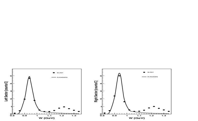
Figure 5: Normalized yields as a function of the invariant mass, $W[{\rm GeV}]$ over $0.08<Q^{2}<0.38\,{\rm GeV}^{2}$. The dots show the BLAST ABS hydrogen data corrected for the background contributions, and the solid line represents the Monte Carlo simulations with radiative effects (ELRADGEN 2.0).

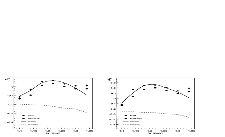
Figure 6: The effect of the radiative contributions to the asymmetry in the $\Delta$-excitation region. The left (left) and right (right) asymmetries are shown with (dots) and without (squares) radiative corrections (RC), for $0.08<Q^{2}<0.38\,{\rm GeV^{2}}$. Monte Carlo simulations using the MAID 2003 model [27] (straight line) and ELRADGEN (dotted line) are shown for comparison.

In order to estimate the contribution of the elastic radiative tail to the $\Delta$-excitation region, the results of the Monte Carlo simulations were normalized to the data elastic peak, as shown in Fig. 5. In this figure, the normalized yields correspond to the outgoing electrons detected in each sector of the BLAST detector (inclusive scattering). The radiative tail obtained from the above normalization is subtracted from the measured yields (radiative corrections), and then the left and right asymmetries are extracted. For comparison, in Fig. 6 we show the left and right asymmetries with and without the radiative corrections. The asymmetry from ELRADGEN alone is also shown (dotted line) in order to see the radiative tail effect to the overall asymmetries and its spin dependence.

6 Conclusion

In this paper, we presented a new version of Monte Carlo generator ELRADGEN for simulation of real-photon events within elastic lepton nucleon scattering for longitudinally polarized lepton and arbitrary polarized target. Following the absolute necessity of both accuracy and quickness for our program, we have developed the fast and highly precise code using analytical integration wherever it was possible. The developed program has a broad spectrum of applications in data analysis of various experimental designs on polarized $ep$-scattering, including the measurements of the generalized parton distributions, the generalized polarizabilities, and the evaluation of spin asymmetries in elastic scattering. Also, it can be used as a generator of the “Born” process in DVCS measurements and of the radiative tail from the elastic peak in DIS. The most significant application of the generator is in the experiments with the complex detector geometry.

The set of numerical tests of the presented version of this code proved its high quality. First, a good agreement with FORTRAN code MASCARAD [11] was found. Second, no dependence on the missing mass square resolution was found. Third, the distributions of the generated radiative events are found to be in accordance with the corresponding probability densities. Fourth, a good agreement with the radiative tail from the elastic peak measured in the BLAST experiment was demonstrated.

Several additional steps allowing to make the simulation even faster are planned. They include implementation of analytical integration over variable $v$ of the hard-photon emission contribution with the longitudinally polarized target and utilizing the look-up table option for faster simulation of radiative events with transverse component of the target polarization vector.

The spectrum of applications of the presented code could be extended after a certain substantive upgrade in several directions including the development of this generator for transferred polarization from lepton beam to recoil proton [28], and for involving this generator into the measurement of the electromagnetic form-factors of the proton in elastic scattering with unpolarized [29] and polarized targets [30, 31]. Inclusion of electroweak effects will provide the generalization for the investigation of electroweak corrections in experiments on axial form factors of the nucleon [32] and parity violation elastic scattering [33]. This generator can be included in data analysis of experiments with the measurement of unpolarized and spin-flip generalized polarizabilities in virtual Compton scattering [3, 4].

Appendix Appendix A Four-vectors

In this section we present the explicit expression for four-vectors decomposition in LAB system depicted in Fig. 7

\begin{picture}(80.0,80.0)\put(10.0,0.0){ \epsfbox{figures/vects2.eps} } \end{picture}

Figure 7: 3-vectors decomposition in the LAB system

Appendix A.1 Polarization vector definitions

As it was mentioned above we assume that the electron beam has a longitudinal polarization. Therefore its polarization vector has a form [19]:

$$\xi_{L}=\frac{1}{\sqrt{\lambda_{s}}}\left(\frac{S}{m}k_{1}-2mp_{1}\right).$$ (A.1)

The target polarization vector in the Lab. system can be decomposed into longitudinal

$$\eta_{L}=\frac{1}{\sqrt{\lambda_{s}}}\left(2Mk_{1}-\frac{S}{M}p_{1}\right)$$ (A.2)

and transverse $\eta_{T}$ components as it is depicted in Fig. 7

$$\eta=\cos(\theta_{\eta})\eta_{L}+\sin(\theta_{\eta})\eta_{T},$$ (A.3)

where $\theta_{\eta}$ is the angle between 3-vectors ${\bf k_{1}}$ and ${\boldsymbol{\eta}}$. Transverse $\eta_{T}$ component can be presented as:

$$\eta_{T}=\cos(\phi-\phi_{\eta})\eta_{t}+\sin(\phi-\phi_{\eta})\eta_{\bot},$$ (A.4)

where $\phi_{\eta}$ is the angle between (${\bf k_{1}}$, ${\boldsymbol{\eta}}$) and OZX planes, and

$$\eta_{t} = \frac{(4m^{2}M^{2}+2Q^{2}M^{2}-SX)k_{1}+\lambda_{s}k_{2}-(SQ^{2}+2m^{2}S_{x})p_{1}}{\sqrt{\lambda\lambda_{s}}},$$

$$\eta_{\bot} = \left(0,\frac{\bf{k_{2}}\times\bf{k_{1}}}{|\bf{k_{2}}||\bf{k_{1}}|\sin\theta}\right)=(0,\sin\phi,-\cos\phi,0).$$ (A.5)

Here

$$X=2k_{2}p_{1},\;S_{x}=S-X,\;\lambda=SXQ^{2}-M^{2}Q^{4}-m^{2}\lambda_{q},$$

$$\lambda_{q}=S_{x}^{2}+4Q^{2}M^{2}.$$ (A.6)

It should be noted, that for the BSV process the variable $X$ is fixed by $Q^{2}$ and $S$: $X=S-Q^{2}$, while for the radiative one, the variable $X$ (as well as $S_{x}$ and $\lambda_{q}$) depends on inelasticity:

$$X=S-Q^{2}-v,\;S_{x}=Q^{2}+v,\;\lambda_{q}=(Q^{2}+v)+4Q^{2}M^{2}.$$ (A.7)

As it follows from (A.9) the normal to scattering plane component of $\eta$ satisfies the equations:

$$k_{1}\eta_{\bot}=k_{2}\eta_{\bot}=p_{1}\eta_{\bot}=0,\;\;k\eta_{\bot}=-p_{2}\eta_{\bot}=\sin\phi_{k}\frac{\sqrt{\lambda_{3}}}{\sqrt{\lambda_{q}}}.$$ (A.8)

Appendix A.2 Four-momenta reconstruction

After generation of photonic variable $t$, $v$ and $\phi_{k}$ the four-momenta of final proton $\displaystyle p_{2}=(p_{2}^{(0)},p_{2}^{(1)},p_{2}^{(2)},p_{2}^{(3)})$, lepton $\displaystyle k_{2}=(k_{2}^{(0)},k_{2}^{(1)},k_{2}^{(2)},k_{2}^{(3)})$ and real photon $\displaystyle k=(k^{(0)},k^{(1)},k^{(2)},k^{(3)})$ in the LAB system read:

$$p^{(1)}_{2}=\frac{\sqrt{\lambda_{3}}(\lambda_{1}\cos\phi\cos\phi_{k}-\sqrt{\lambda_{q}}S\sin\phi\sin\phi_{k})+\lambda_{2}\sqrt{\lambda_{4}}\cos\phi}{\lambda_{q}S},$$

$$p^{(2)}_{2}=\frac{\sqrt{\lambda_{3}}(\sqrt{\lambda_{q}}S\cos\phi\sin\phi_{k}+\lambda_{1}\sin\phi\cos\phi_{k})+\lambda_{2}\sqrt{\lambda_{4}}\sin\phi}{\lambda_{q}S},$$

$$p^{(3)}_{2}=\frac{\lambda_{1}\lambda_{2}-4M^{2}\sqrt{\lambda_{3}\lambda_{4}}\cos\phi_{k}}{2\lambda_{q}MS},\;p_{2}^{(0)}=\frac{t+2M^{2}}{2M},$$

$$k_{2}^{(1)}=\frac{\sqrt{\lambda_{4}}\cos\phi}{S},\;k_{2}^{(2)}=\frac{\sqrt{\lambda_{4}}\sin\phi}{S},\;k_{2}^{(3)}=\frac{S^{2}-\lambda_{1}}{2MS},\;k_{2}^{(0)}=\frac{S-Q^{2}-v}{2M},$$

$$k^{(1)}=\frac{\sqrt{\lambda_{3}}(\sqrt{\lambda_{q}}S\sin\phi\sin\phi_{k}-\lambda_{1}\cos\phi\cos\phi_{k})+(\lambda_{q}-\lambda_{2})\sqrt{\lambda_{4}}\cos\phi}{\lambda_{q}S},$$

$$k^{(2)}=\frac{-\sqrt{\lambda_{3}}(\sqrt{\lambda_{q}}S\cos\phi\sin\phi_{k}+\lambda_{1}\sin\phi\cos\phi_{k})+(\lambda_{q}-\lambda_{2})\sqrt{\lambda_{4}}\sin\phi}{\lambda_{q}S},$$

$$k^{(3)}=\frac{\lambda_{1}(\lambda_{q}-\lambda_{2})+4M^{2}\sqrt{\lambda_{3}\lambda_{4}}\cos\phi_{k}}{2\lambda_{q}MS},\;k^{(0)}=\frac{Q^{2}+v-t}{2M},$$ (A.9)

where

$$\lambda_{1}=S(Q^{2}+v)+2M^{2}Q^{2},\;\qquad\qquad \lambda_{2}=t(Q^{2}+v)+2M^{2}(Q^{2}+t),$$

$$\lambda_{3}=tv(Q^{2}-t+v)-M^{2}(Q^{2}-t)^{2},\; \lambda_{4}=Q^{2}S(v_{max}-v).$$ (A.10)

Appendix Appendix B Explicit expressions for the kinematic quantities $\theta$

The kinematic coefficients $\theta_{i}^{B}$ appear as a convolution of the leptonic tensor $L_{\mu\nu}^{B}$ with corresponding hadronic structures

$$w^{\mu\nu}_{1}=-g_{\mu\nu},\qquad\qquad\qquad\;\;w^{\mu\nu}_{2}=\frac{p_{\mu}p_{\nu}}{M^{2}},$$

$$w^{\mu\nu}_{3}=-iP_{N}\epsilon_{\mu\nu\lambda\sigma}{q_{\lambda}\eta_{\sigma}\over M},\qquad w^{\mu\nu}_{4}=iP_{N}\epsilon_{\mu\nu\lambda\sigma}{q_{\lambda}p_{\sigma}\;\eta q\over M^{3}}$$ (B.11)

and read

$$\theta_{1}^{B}=\frac{1}{2}L^{B}_{\mu\nu}w_{1}^{\mu\nu}=Q^{2},$$

$$\theta_{2}^{B}=\frac{1}{2}L^{B}_{\mu\nu}w_{2}^{\mu\nu}=\frac{1}{2M^{2}}(S(S-Q^{2})-M^{2}Q^{2}),$$

$$\theta_{3}^{B}=\frac{1}{2}L^{B}_{\mu\nu}w_{3}^{\mu\nu}=P_{L}P_{N}\frac{2m}{M}(q\eta\;k_{2}\xi-\xi\eta\;Q^{2}),$$

$$\theta_{4}^{B}=\frac{1}{2}L^{B}_{\mu\nu}w_{4}^{\mu\nu}=P_{L}P_{N}\frac{mQ^{2}\;q\eta}{M^{3}}(2p_{1}\xi-k_{2}\xi).$$ (B.12)

Here $P_{L}$ and $P_{N}$ define the degree of the lepton and target polarization respectively and the explicit expressions for polarized vectors of the scattering particles $\xi$ and $\eta$ can be found in Appendix A.1.

The quantities $\theta_{i}(v_{1},v_{2})$ appear as a convolution of the leptonic tensor that is responsible for the real photon emission:

$$L_{\mu\nu}^{R} = -\frac{1}{2}{\rm Tr}[({\hat{k}}_{2}+m)\Gamma_{\mu\alpha}(1-P_{L}{\hat{\xi}}\gamma_{5})({\hat{k}}_{1}+m){\hat{\Gamma}}_{\alpha\nu}],$$

$$\Gamma_{\mu\alpha} = \left(\frac{k_{1\alpha}}{kk_{1}}-\frac{k_{2\alpha}}{kk_{2}}\right)\gamma_{\mu}-\frac{\gamma_{\mu}{\hat{k}}\gamma_{\alpha}}{2kk_{1}}-\frac{\gamma_{\alpha}{\hat{k}}\gamma_{\mu}}{2kk_{2}},\;$$

$$\hat{\Gamma}_{\alpha\nu} = \left(\frac{k_{1\alpha}}{kk_{1}}-\frac{k_{2\alpha}}{kk_{2}}\right)\gamma_{\nu}-\frac{\gamma_{\alpha}{\hat{k}}\gamma_{\nu}}{2kk_{1}}-\frac{\gamma_{\nu}{\hat{k}}\gamma_{\alpha}}{2kk_{2}}$$ (B.13)

with hadronic structures presented in eq.(B.11).

As a result

$$\theta_{i}^{R}(v_{1},v_{2}) = -\frac{1}{4\pi}\int\limits_{v_{1}}^{v_{2}}\frac{dv}{\sqrt{\lambda_{q}}}\int\limits_{0}^{2\pi}d\phi_{k}\ L^{R}_{\mu\nu}w_{i}^{\mu\nu}(q\to q-k)=\sum_{j=1}^{k_{i}}\int\limits_{v_{1}}^{v_{2}}dvR^{j-3}\theta_{ij}^{R}(v)$$ (B.14)

$$= \sum_{j=1}^{k_{i}}\int\limits_{v_{1}}^{v_{2}}dv\int\limits_{0}^{2\pi}d\phi_{k}\ R^{j-3}\theta_{ij}^{R}(v,\phi_{k}),\;$$

where $R$ and $k_{i}$ are defined after eq. (12).

Appendix B.1 Quantities $\theta_{ij}(v)$ and $\theta_{ij}(v,\phi_{k})$

Here, we combine explicit expressions for $\theta_{ij}^{R}(v)$ and $\theta_{ij}^{R}(v,\phi_{k})$ quantities calculated for polarized scattering [5, 19, 34] and present the explicit expressions $\theta_{i}^{R}(v_{1},v_{2})$ calculated for unpolarized scattering only.

Both types of quantities $\theta_{ij}^{R}(v)$ and $\theta_{ij}^{R}(v,\phi_{k})$ for $i=1,2,3$ take the similar form

$$\theta_{11}^{R} = 4Q^{2}F_{IR},$$

$$\theta_{12}^{R} = 4\tau F_{IR},$$

$$\theta_{13}^{R} = -4F-2\tau^{2}F_{d},$$

$$\theta_{21}^{R} = {2(SX-M^{2}Q^{2})F_{IR}/M^{2}},$$

$$\theta_{22}^{R} = (2m^{2}S_{p}F_{2-}+S_{p}S_{x}F_{1+}+2(S_{x}-2M^{2}\tau)F_{IR}-\tau S^{2}_{p}F_{d})/2M^{2},$$

$$\theta_{23}^{R} = (4M^{2}F+(2M^{2}\tau-S_{x})\tau F_{d}-S_{p}F_{1+})/2M^{2},$$

$$\theta_{31}^{R} = P_{L}P_{N}{8m\over M}(\eta q\;k_{2}\xi-Q^{2}\;\xi\eta)F_{IR},$$

$$\theta_{32}^{R} = -P_{L}P_{N}{2m\over M}(2\eta q\;(\tau k_{2}\xi F_{d}-2F^{\xi}_{IR})+Q^{2}\eta{\mathcal{K}}(F^{\xi}_{2+}-F^{\xi}_{-2}-2F^{\xi}_{d})$$

$$+4\xi\eta\tau F_{IR}-4m^{2}k_{2}\xi(2F^{\eta}_{d}-F^{\eta}_{2+}))$$

$$\theta_{33}^{R} = P_{L}P_{N}{2m\over M}(\eta{\mathcal{K}}\;\tau(2F^{\xi}_{d}+F^{\xi}_{2-}-F^{\xi}_{2+})-2\;k_{2}\xi\;\tau F^{\eta}_{d}-4m^{2}F^{\xi\eta}_{d}-6F^{\xi\eta}_{IR}$$

$$+Q^{2}(F^{\xi\eta}_{2+}-F^{\xi\eta}_{2-})),$$

$$\theta_{34}^{R} = P_{L}P_{N}{2m\tau\over M}\pmatrix{2F^{\xi\eta}_{d}+F^{\xi\eta}_{2+}-F^{\xi\eta}_{2-}},$$ (B.15)

where $\tau=(t-Q^{2})/R$ and the four-vector ${\mathcal{K}}=k_{1}+k_{2}$.

For $i=4$ we have

$$\theta_{41}^{R}=\eta q{\widetilde{\theta}_{41}}/M,\qquad\qquad\;\; \theta_{42}^{R}=(\eta q{\widetilde{\theta}}_{42}-\widetilde{\theta}_{41}^{\eta})/M,$$

$$\theta_{43}^{R}=(\eta q{\widetilde{\theta}}_{43}-\widetilde{\theta}_{42}^{\eta})/M,\;\;\;\;\;\; \theta_{44}^{R}=(\eta q{\widetilde{\theta}}_{44}-\widetilde{\theta}_{43}^{\eta})/M,$$

$$\theta_{45}^{R}=-\widetilde{\theta}_{44}^{\eta}/M,\qquad\qquad\;\;\;\;$$ (B.16)

where

$${\widetilde{\theta}}_{41} = P_{L}P_{N}{4m\over M^{2}}\pmatrix{2\;\xi p\;Q^{2}-S_{x}\;\xi k_{2}}F_{IR},$$

$${\widetilde{\theta}}_{42} = P_{L}P_{N}{m\over M^{2}}(2\pmatrix{S_{p}-2S_{x}}F^{\xi}_{IR}+2\;k_{2}\xi\;\tau S_{x}F_{d}+8\;\xi p\;\tau F_{IR}$$

$$+S_{p}\pmatrix{Q^{2}_{m}F^{\xi}_{2+}-Q^{2}F^{\xi}_{2-}}-4m^{2}(\;k_{2}\xi\;(2F_{d}-F_{2+})+S_{p}(F^{\xi}_{2+}-F^{\xi}_{d})),$$

$${\widetilde{\theta}}_{43} = P_{L}P_{N}{m\over M^{2}}(\pmatrix{Q^{2}-\tau S_{p}}F^{\xi}_{2-}-\pmatrix{Q^{2}_{m}-\tau S_{p}}F^{\xi}_{2+}+2\;k_{2}\xi\;\tau F_{d}$$

$$+6F^{\xi}_{IR}-2F^{\xi}_{d}\tau S_{p}),$$

$${\widetilde{\theta}}_{44} = -P_{L}P_{N}{m\tau\over M^{2}}\pmatrix{2F^{\xi}_{d}-F^{\xi}_{2-}+F^{\xi}_{2+}}.$$ (B.17)

The quantities ${\widetilde{\theta}}_{4j}^{\eta}$ are calculated as:

$${\widetilde{\theta}}_{4j}^{\eta}={\widetilde{\theta}}_{4j}(F_{all}\to F_{all}^{\eta},F_{all}^{\xi}\to F_{all}^{\xi\eta}).$$ (B.18)

The upper indices in $F_{all}$ appears in the following way:

$$2F_{2+}^{\xi} = (2F_{1+}+\tau F_{2-})s_{\xi}+F_{2+}r_{\xi},$$

$$2F_{2+}^{\eta} = (2F_{1+}+\tau F_{2-})s_{\eta}+F_{2+}r_{\eta}+\frac{4\sin\phi_{k}d_{\eta}}{R}\sqrt{\frac{\lambda_{3}}{\lambda_{q}}}F_{2+},$$

$$2F_{2-}^{\xi} = (2F_{d}+F_{2+})\tau s_{\xi}+F_{2-}r_{\xi},$$

$$2F_{d}^{\xi} = F_{1+}s_{\xi}+F_{d}r_{\xi},$$

$$2F_{d}^{\eta} = F_{1+}s_{\eta}+F_{d}r_{\eta}+\frac{4\sin\phi_{k}d_{\eta}}{R}\sqrt{\frac{\lambda_{3}}{\lambda_{q}}}F_{d},$$

$$4F_{2+}^{\xi\eta} = (2F_{1+}+\tau F_{2-})(r_{\eta}s_{\xi}+s_{\eta}r_{\xi})+F_{2+}(r_{\eta}r_{\xi}+\tau^{2}s_{\eta}s_{\xi})$$

$$+4(2F+F_{d}\tau^{2})s_{\eta}s_{\xi}+\frac{8\sin\phi_{k}d_{\eta}}{R}\sqrt{\frac{\lambda_{3}}{\lambda_{q}}}F_{2+}^{\xi},$$

$$4F_{2-}^{\xi\eta} = (2F_{d}+F_{2+})(r_{\eta}s_{\xi}+s_{\eta}r_{\xi})+F_{2-}(r_{\eta}r_{\xi}+\tau^{2}s_{\eta}s_{\xi})+4\tau F_{1+}s_{\eta}s_{\xi}$$

$$+\frac{8\sin\phi_{k}d_{\eta}}{R}\sqrt{\frac{\lambda_{3}}{\lambda_{q}}}F_{2-}^{\xi},$$

$$4F_{d}^{\xi\eta} = F_{1+}(r_{\eta}s_{\xi}+s_{\eta}r_{\xi})+F_{d}(r_{\eta}r_{\xi}+\tau^{2}s_{\eta}s_{\xi})+4Fs_{\eta}s_{\xi}$$ (B.19)

$$+\frac{8\sin\phi_{k}d_{\eta}}{R}\sqrt{\frac{\lambda_{3}}{\lambda_{q}}}F_{d}^{\xi}.$$

The quantities

$$s_{\{\xi,\eta\}}=a_{\{\xi,\eta\}}+b_{\{\xi,\eta\}},r_{\{\xi,\eta\}}=\tau(a_{\{\xi,\eta\}}-b_{\{\xi,\eta\}})+2c_{\{\xi,\eta\}}$$ (B.20)

are combinations of coefficients of polarization vectors $\xi$ and $\eta$ expansion over basis (see Appendix A.1)

$$\xi = 2(a_{\xi}k_{1}+b_{\xi}k_{2}+c_{\xi}p),$$

$$\eta = 2(a_{\eta}k_{1}+b_{\eta}k_{2}+c_{\eta}p+d_{\eta}\eta_{\bot}).$$ (B.21)

We note that the scalar products from (B.15,B.16,B.17) are also calculated in terms of the polarization vector coefficients:

$$\eta q=-Q^{2}(a_{\eta}-b_{\eta})+S_{x}c_{\eta},\quad\eta{\mathcal{K}}=(Q^{2}+4m^{2})(a_{\eta}+b_{\eta})+S_{p}c_{\eta},$$

$$k_{2}\xi=Q^{2}_{m}a_{\xi}+2m^{2}b_{\xi}+Xc_{\xi},\quad\xi p=Sa_{\xi}+Xb_{\xi}+2M^{2}c_{\xi},$$

$$\frac{1}{2}\xi\eta=2m^{2}(a_{\xi}a_{\eta}+b_{\xi}b_{\eta})+2M^{2}c_{\xi}c_{\eta}+Q_{m}^{2}(a_{\xi}b_{\eta}+b_{\xi}a_{\eta})$$

$$+S(a_{\xi}c_{\eta}+c_{\xi}a_{\eta})+X(b_{\xi}c_{\eta}+c_{\xi}b_{\eta}).$$ (B.22)

With the exception of the contribution proportional to $d_{\eta}$ all dependencies of $\theta_{ij}$ on the photonic variable $\phi_{k}$ are included in the quantities $F$, however in both cases we have:

$$F_{IR}=m^{2}F_{2+}-Q^{2}F_{d}$$ (B.23)

So for $\theta_{ij}(v,\phi_{k})$ the quantities $F$ read

$$F_{d}(v,\phi_{k})=\frac{F(v,\phi_{k})}{z_{1}z_{2}},\qquad\qquad\;\;\;\;F_{1+}(v,\phi_{k})=F(v,\phi_{k})\left(\frac{1}{z_{1}}+\frac{1}{z_{2}}\right),$$

$$F_{2\pm}(v,\phi_{k})=F(v,\phi_{k})\left(\frac{1}{z_{2}^{2}}\pm\frac{1}{z_{1}^{2}}\right),\;F(v,\phi_{k})=\frac{1}{2\pi\sqrt{\lambda_{q}}}.$$ (B.24)

Here

$$z_{1} = \frac{2kk_{1}}{R}=\frac{1}{\lambda_{q}}(Q^{2}S_{p}+\tau(SS_{x}+2M^{2}Q^{2})-2M\sqrt{\lambda_{z}}\cos\phi_{k}),$$

$$z_{2} = \frac{2kk_{2}}{R}=\frac{1}{\lambda_{q}}(Q^{2}S_{p}+\tau(XS_{x}-2M^{2}Q^{2})-2M\sqrt{\lambda_{z}}\cos\phi_{k}),$$ (B.25)

and

$$\lambda_{z}=(\tau-\tau_{min})(\tau_{max}-\tau)\lambda,\qquad\tau_{max/min}=\frac{S_{x}\pm\sqrt{\lambda_{q}}}{2M^{2}},$$

$$S_{p}=S+X=2S-Q^{2}-v.$$ (B.26)

The following equalities define the functions $F$ for $\theta_{ij}^{R}(v)$:

$$F(v)=\lambda^{-1/2}_{q},\;F_{d}(v)=\tau^{-1}(C^{-1/2}_{2}(\tau)-C^{-1/2}_{1}(\tau)),$$

$$F_{1+}(v)=C^{-1/2}_{2}(\tau)+C^{-1/2}_{1}(\tau),$$

$$F_{2\pm}(v)=B_{2}(\tau)C^{-3/2}_{2}(\tau)\mp B_{1}(\tau)C^{-3/2}_{1}(\tau),$$ (B.27)

where

$$B_{1,2}(\tau)=-{1\over 2}\pmatrix{\lambda_{q}\tau\pm S_{p}(S_{x}\tau+2Q^{2})},$$

$$C_{1}(\tau)=(S\tau+Q^{2})^{2}+4m^{2}(Q^{2}+\tau S_{x}-\tau^{2}M^{2}),$$

$$C_{2}(\tau)=(X\tau-Q^{2})^{2}+4m^{2}(Q^{2}+\tau S_{x}-\tau^{2}M^{2}).$$ (B.28)

We note that $F_{d}$ has a $0/0$-like uncertainty for $\tau=0$ (inside the integration region). It leads to difficulties in numerical integration, so another form is used also

$$F_{d}(v)={S_{p}(\tau S_{x}+2Q^{2})\over{C_{1}^{1/2}(\tau)}{C_{2}^{1/2}(\tau)}({C_{1}^{1/2}(\tau)}+{C^{1/2}_{2}(\tau)})}.$$ (B.29)

Appendix B.2 Quantities $\theta_{i}^{R}(v_{1},v_{2})$

As it was mentioned above for the unpolarized scattering, the integration over $v$ is performed analytically resulting in:

$$\theta_{1}^{R}(v_{1},v_{2}) = -4I_{F}+4tI^{-2}_{2+}-2(Q^{4}+t^{2})I^{-2}_{d},$$

$$\theta_{2}^{R}(v_{1},v_{2}) = \frac{1}{2M^{2}}(4M^{2}I_{F}-t(I_{1+}^{0}+2I_{d}^{0})+t(2S-t)I_{1+}^{-1}+4I_{21}^{0}$$ (B.30)

$$-4(2S-t)I_{21}^{-1}+4(S^{2}-t(M^{2}+S))I_{2+}^{-2}$$

$$+t(Q^{2}+4S-3t)I_{d}^{-1}$$

$$+[t(Q^{2}t-(2S-t)^{2})+2M^{2}(t^{2}+Q^{4})]I_{d}^{-2}),$$

where

$$I_{F} = \int\limits^{v_{2}}_{v_{1}}dvF(v)=\log\left(\frac{Q^{2}+v_{2}+\sqrt{(Q^{2}+v_{2})^{2}+4M^{2}Q^{2}}}{Q^{2}+v_{1}+\sqrt{(Q^{2}+v_{1})^{2}+4M^{2}Q^{2}}}\right),$$

$$I_{1+}^{0} = \int\limits^{v_{2}}_{v_{1}}dvF_{1+}(v)=(Q^{2}-t)\left(\frac{S}{Q^{4}}\Delta L_{1}-\frac{S-t}{t^{2}}\Delta L_{2}\right)+\frac{\Delta_{1}^{1}}{Q^{4}}+\frac{\Delta_{2}^{1}}{t^{2}},$$

$$I_{1+}^{-1} = \int\limits^{v_{2}}_{v_{1}}\frac{dv}{R}F_{1+}(v)=\frac{1}{Q^{2}}\Delta L_{1}+\frac{1}{t}\Delta L_{2},$$

$$I_{21}^{0} = \frac{1}{2}m^{2}\int\limits^{v_{2}}_{v_{1}}dv(F_{2+}(v)-F_{2-}(v))=\frac{1}{2}(Q^{2}-t)\frac{S^{2}}{Q^{4}}\Delta_{1}^{0},$$

$$I_{21}^{-1} = \frac{1}{2}m^{2}\int\limits^{v_{2}}_{v_{1}}\frac{dv}{R}(F_{2+}(v)-F_{2-}(v))=\frac{S}{2Q^{2}}\Delta_{1}^{0},$$

$$I_{2+}^{-2} = m^{2}\int\frac{dv}{R^{2}}F_{2+}(v)=\frac{1}{2(Q^{2}-t)}\left(\Delta_{1}^{0}-\frac{Q^{2}}{t}\Delta_{2}^{0}\right),$$

$$I_{d}^{0} = \int\limits^{v_{2}}_{v_{1}}dvF_{d}(v)=(Q^{2}-t)\left(\frac{S^{2}}{Q^{6}}\Delta L_{1}-\frac{(S-t)^{2}}{t^{3}}\Delta L_{2}\right)+2\frac{S}{Q^{6}}\Delta_{1}^{1}$$

$$+2\frac{S-t}{t^{3}}\Delta_{2}^{1}+\frac{1}{2(Q^{2}-t)}\left(\frac{\Delta_{1}^{2}}{Q^{6}}-\frac{\Delta_{2}^{2}}{t^{3}}\right),$$

$$I_{d}^{-1} = \int\limits^{v_{2}}_{v_{1}}\frac{dv}{R}F_{d}(v)=\frac{S}{Q^{4}}\Delta L_{1}+\frac{S-t}{t^{2}}\Delta L_{2}+\frac{1}{Q^{2}-t}\left(\frac{\Delta_{1}^{1}}{Q^{4}}-\frac{\Delta_{2}^{1}}{t^{2}}\right),$$

$$I_{d}^{-2} = \int\limits^{v_{2}}_{v_{1}}\frac{dv}{R^{2}}F_{d}(v)=\frac{1}{Q^{2}-t}\left(\frac{1}{Q^{2}}\Delta L_{1}-\frac{1}{t}\Delta L_{2}\right).$$ (B.31)

Here

$$\Delta_{i}^{2}=|D_{i}(v_{2})|D_{i}(v_{2})-|D_{i}(v_{1})|D_{i}(v_{1}),\;\Delta_{i}^{1}=|D_{i}(v_{2})|-|D_{i}(v_{1})|,$$

$$\Delta_{i}^{0}=D_{i}(v_{2})/D^{2}_{i+3}(v_{2})-D_{i}(v_{1})/D^{2}_{i+3}(v_{1}),$$ (B.32)

$$\Delta L_{1}=\log\Biggl{[}\frac{2m^{2}t(Q^{2}-t+2v_{2})+Q^{2}D_{1}(v_{2})+D_{4}(v_{2})\sqrt{4m^{2}t+Q^{4}}}{2m^{2}t(Q^{2}-t+2v_{1})+Q^{2}D_{1}(v_{1})+D_{4}(v_{1})\sqrt{4m^{2}t+Q^{4}}}\Biggr{]},$$

$$\Delta L_{2}=\log\Biggl{[}\frac{2m^{2}\sqrt{t}(Q^{2}-t+2v_{2})+\sqrt{t}D_{2}(v_{2})+D_{5}(v_{2})\sqrt{4m^{2}+t}}{2m^{2}\sqrt{t}(Q^{2}-t+2v_{1})+\sqrt{t}D_{2}(v_{1})+D_{5}(v_{1})\sqrt{4m^{2}+t}}\Biggr{]}$$

and

$$D_{1}(v) = (t-Q^{2})(S-Q^{2})+Q^{2}v,$$

$$D_{2}(v) = S(Q^{2}-t)+tv,$$

$$D_{3}(v) = vt(v-t+Q^{2})-M^{2}(Q^{2}-t)^{2},$$

$$D_{4}(v) = \sqrt{D^{2}_{1}(v)+4m^{2}D_{3}(v)},$$

$$D_{5}(v) = \sqrt{D^{2}_{2}(v)+4m^{2}D_{3}(v)}.$$ (B.33)

Appendix Appendix C Test output

Here, we present the results of the test as test.dat output file corresponding to:
1) $itest:=1$ – the generation of $\rho(t)$ distribution and comparison with the analytical cross section corresponding to the first formula in (15) (here and below invariants $v,t$ are in $\mbox{GeV}^{2}$)

itest=1
t    generation
rgen is generated probability
rcalc is calculated probability
Ebeam=.850     GeV
Q**2=.200     GeV**2
vmin=0.10E-01 GeV**2
vcut=0.00     GeV**2
PL*PN=-1.00    lepton polarization times nucleon polarization
thetapn=48.0    degrees angle between target polarization
                vector and beam momentum in Lab system
phipn=0.00     degrees athimutal angle  in Lab system
number of bins 20
number of radiative events   100000000
initial random number 12
bin      t          rgen        rcalc        rgen/rcalc
       GeV**2           GeV**(-2)
  1   0.4237E-01    1.624        1.786       0.9093
  2   0.9197E-01    1.619        1.589        1.019
  3   0.1453        2.325        2.274        1.023
  4   0.1969        12.14        35.10       0.3460
  5   0.2351        1.518        1.666       0.9108
  6   0.2893       0.3042       0.3153       0.9647
  7   0.3411       0.1113       0.1134       0.9816
  8   0.3923       0.5102E-01   0.5163E-01   0.9883
  9   0.4433       0.2666E-01   0.2688E-01   0.9917
 10   0.4943       0.1518E-01   0.1526E-01   0.9945
 11   0.5449       0.9216E-02   0.9259E-02   0.9954
 12   0.5960       0.5872E-02   0.5865E-02    1.001
 13   0.6466       0.3893E-02   0.3872E-02    1.006
 14   0.6973       0.2577E-02   0.2632E-02   0.9791
 15   0.7479       0.1822E-02   0.1833E-02   0.9937
 16   0.7983       0.1278E-02   0.1304E-02   0.9801
 17   0.8490       0.9465E-03   0.9396E-03    1.007
 18   0.9003       0.6965E-03   0.6806E-03    1.023
 19   0.9509       0.4965E-03   0.4945E-03    1.004
 20   0.9973       0.2696E-03   0.3558E-03   0.7577

2) $itest:=2$ – the generation of $\rho(v)$ distribution and comparison with the analytical cross section corresponding to the second formula in (15)

itest=2
v    generation
rgen is generated probability
rcalc is calculated probability
Ebeam=.850     GeV
Q**2=.200     GeV**2
vmin=0.10E-01 GeV**2
vcut=0.00     GeV**2
PL*PN=-1.00    lepton polarization times nucleon polarization
thetapn=48.0    degrees angle between target polarization
                vector and beam momentum in Lab system
phipn=0.00     degrees athimutal angle  in Lab system
number of bins 20
number of radiative events   100000000
initial random number 12
 t= 0.5218    GeV**2
bin      v          rgen        rcalc        rgen/rcalc
       GeV**2           GeV**(-2)
  1   0.6260       0.1660       0.1657        1.002
  2   0.6599       0.1931       0.1933       0.9990
  3   0.6937       0.2265       0.2266       0.9998
  4   0.7275       0.2676       0.2677       0.9996
  5   0.7613       0.3206       0.3205        1.000
  6   0.7952       0.3904       0.3913       0.9978
  7   0.8291       0.4927       0.4921        1.001
  8   0.8630       0.6478       0.6486       0.9987
  9   0.8971       0.9284       0.9278        1.001
 10   0.9316        1.579        1.580       0.9993
 11   0.9698        6.013        6.043       0.9951
 12   0.9886        13.45        16.44       0.8179
 13    1.029        1.759        1.760       0.9992
 14    1.064       0.9512       0.9502        1.001
 15    1.098       0.6343       0.6361       0.9973
 16    1.132       0.4694       0.4686        1.002
 17    1.166       0.3649       0.3645        1.001
 18    1.199       0.2937       0.2942       0.9985
 19    1.233       0.2435       0.2436       0.9999
 20    1.267       0.2071       0.2053        1.008

3) $itest:=3$ – the generation of $\rho(\phi_{k})$ distribution and comparison with the analytical cross section corresponding to the third formula in (15)

itest=3
phik generation
rgen is generated probability
rcalc is calculated probability
Ebeam=.850     GeV
Q**2=.200     GeV**2
vmin=0.10E-01 GeV**2
vcut=0.00     GeV**2
PL*PN=-1.00    lepton polarization times nucleon polarization
thetapn=48.0    degrees angle between target polarization
                vector and beam momentum in Lab system
phipn=0.00     degrees athimutal angle  in Lab system
number of bins 20
number of radiative events   100000000
initial random number 12
 t= 0.5218    GeV**2
 v= 0.7962    GeV**2
bin      phik       rgen        rcalc        rgen/rcalc
         rad             rad**(-1)
  1   -2.984       0.1890E-01   0.1884E-01    1.003
  2   -2.668       0.2043E-01   0.2036E-01    1.004
  3   -2.351       0.2388E-01   0.2381E-01    1.003
  4   -2.035       0.3031E-01   0.3027E-01    1.001
  5   -1.718       0.4189E-01   0.4197E-01   0.9980
  6   -1.402       0.6354E-01   0.6381E-01   0.9959
  7   -1.085       0.1062       0.1069       0.9927
  8  -0.7682       0.1961       0.1988       0.9864
  9  -0.4529       0.3922       0.4013       0.9773
 10  -0.1470       0.6982       0.7223       0.9667
 11   0.1470       0.6981       0.7223       0.9665
 12   0.4530       0.3924       0.4012       0.9779
 13   0.7682       0.1960       0.1988       0.9862
 14    1.085       0.1061       0.1069       0.9919
 15    1.402       0.6351E-01   0.6380E-01   0.9955
 16    1.718       0.4192E-01   0.4197E-01   0.9988
 17    2.035       0.3036E-01   0.3026E-01    1.003
 18    2.351       0.2389E-01   0.2381E-01    1.003
 19    2.667       0.2036E-01   0.2036E-01    1.000
 20    2.983       0.1888E-01   0.1884E-01    1.002

4) $itest:=4$ – the cross-check of the accuracy of the vector reconstruction for 5 random radiative events

itest=4
variable reconstruction
Ebeam=.850     GeV
Q**2=.200     GeV**2
vmin=0.10E-01 GeV**2
vcut=0.00     GeV**2
PL*PN=-1.00    beam polarization times target polarization
thetapn=48.0    degrees angle between target polarization
                vector and beam momentum in Lab system
phipn=0.00     degrees athimutal angle  in Lab system
number of bins 20
number of radiative events  5
initial random number 12
 -------------------------------------------
 event=           1
 test v reconstruction
v=0.206247E-01 GeV**2   reconstructed v from 4-vector
v=0.206247E-01 GeV**2   generated v

 test t reconstruction
t=0.202340     GeV**2   reconstructed t from 4-vecto
t=0.202340     GeV**2   generated t

m2gamma= 0.157778E-10    GeV**2  real photon mass square

 -------------------------------------------
 event=           2
 test v reconstruction
v=0.579509     GeV**2   reconstructed v from 4-vector
v=0.579509     GeV**2   generated v

 test t reconstruction
t=0.119041     GeV**2   reconstructed t from 4-vecto
t=0.119041     GeV**2   generated t

m2gamma=-0.855924E-08    GeV**2  real photon mass square

 -------------------------------------------
 event=           3
 test v reconstruction
v=0.328652E-01 GeV**2   reconstructed v from 4-vector
v=0.328652E-01 GeV**2   generated v

 test t reconstruction
t=0.203009     GeV**2   reconstructed t from 4-vecto
t=0.203009     GeV**2   generated t

m2gamma= 0.249049E-10    GeV**2  real photon mass square

 -------------------------------------------
 event=           4
 test v reconstruction
v=0.579878     GeV**2   reconstructed v from 4-vector
v=0.579878     GeV**2   generated v

 test t reconstruction
t=0.117210     GeV**2   reconstructed t from 4-vecto
t=0.117210     GeV**2   generated t

m2gamma=-0.340940E-08    GeV**2  real photon mass square

 -------------------------------------------
 event=           5
 test v reconstruction
v=0.412302E-01 GeV**2   reconstructed v from 4-vector
v=0.412302E-01 GeV**2   generated v

 test t reconstruction
t=0.193803     GeV**2   reconstructed t from 4-vecto
t=0.193803     GeV**2   generated t

m2gamma= 0.124488E-10    GeV**2  real photon mass square

4) $itest:=5$ – the cross-check of the accuracy of the analytical and numerical integration over $t$ for unpolarized scattering

itest=5
comparison of the analytical and numerical integration over t
rnum is the numerically integrated cross section
ran is the analytically integrated cross section
Ebeam=4.00    GeV
Q**2=3.00    GeV**2
vmin=0.10E-01 GeV**2
vcut=.200     GeV**2
PL*PN= 0.00    beam polarization times target polarization
bin      t          rnum          ran         rnum/ran
      GeV**2      nbarn*GeV**(-4)*rad**(-1)
  1    2.340       0.8162E-06   0.8179E-06   0.9979
  2    2.382       0.2651E-05   0.2656E-05   0.9980
  3    2.424       0.4847E-05   0.4857E-05   0.9980
  4    2.466       0.7560E-05   0.7575E-05   0.9981
  5    2.509       0.1102E-04   0.1104E-04   0.9981
  6    2.551       0.1561E-04   0.1564E-04   0.9982
  7    2.593       0.2194E-04   0.2198E-04   0.9983
  8    2.635       0.3111E-04   0.3116E-04   0.9984
  9    2.677       0.4521E-04   0.4528E-04   0.9985
 10    2.720       0.6865E-04   0.6874E-04   0.9986
 11    2.762       0.1122E-03   0.1124E-03   0.9988
 12    2.804       0.2096E-03   0.2098E-03   0.9990
 13    2.846       0.5433E-03   0.5436E-03   0.9994
 14    2.889       0.5977E-02   0.5971E-02    1.001
 15    2.931       0.1018E-01   0.1017E-01    1.001
 16    2.973       0.2645E-01   0.2641E-01    1.002
 17    3.015       0.4498E-01   0.4490E-01    1.002
 18    3.057       0.1006E-01   0.1004E-01    1.001
 19    3.100       0.3106E-03   0.3109E-03   0.9991
 20    3.142       0.2593E-04   0.2598E-04   0.9982

References

- [1] M. Diehl, Phys. Rept. 388, (2003) 41.
- [2] A. Airapetian et al. Nucl. Phys. B 829, (2010) 1.
- [3] P. A. M. Guichon et al., Nucl. Phys. A 591, (1995) 606.
- [4] D. Drechsel et al., Phys. Rev. C 57, (1998) 941.
- [5] I. V. Akushevich and N. M. Shumeiko, J. Phys. G 20 (1994) 513.
- [6] A. Akhundov, D. Bardin, L. Kalinovskaya and T. Riemann, Fortsch. Phys. 44, (1996) 373.
- [7] L. C. Maximon and J. A. Tjon, Phys. Rev. C 62, (2000) 054320.
- [8] L. W. Mo and Y. S. Tsai, Rev. Mod. Phys. 41, (1969) 205.
- [9] R. Ent et al. Phys. Rev. C 64 (2001) 054610.
- [10] D. Yu. Bardin, N.M. Shumeiko: Nucl. Phys. B 127 (1977) 242.
- [11] A. V. Afanasev, I. Akushevich, N. P. Merenkov: Phys. Rev. D 64 (2001) 113009.
- [12] A. V. Afanasev, I. Akushevich, A. Ilyichev, N. P. Merenkov: Phys. Lett. B 514 (2001) 269.
- [13] R. Madey et al. [E93-038 Collaboration], Phys. Rev. Lett. 91, 122002 (2003) [arXiv:nucl-ex/0308007].
- [14] D. I. Glazier et al., Eur. Phys. J. A 24, 101 (2005) [arXiv:nucl-ex/0410026].
- [15] E. A. Kuraev, N. P. Merenkov and V. S. Fadin, Sov. J. Nucl. Phys. 47, (1988) 1009.
- [16] A. V. Afanasev, I. Akushevich and N. P. Merenkov, J. Exp. Theor. Phys. 98, 403 (2004) [Zh. Eksp. Teor. Fiz. 98, 462 (2004)] [arXiv:hep-ph/0111331].
- [17] A. V. Afanasev, I. Akushevich and N. P. Merenkov, Phys. Rev. D 65, 013006 (2002) [arXiv:hep-ph/0009273].
- [18] I. Akushevich, H. Boettcher, D. Ryckbosch, In Proc. Workshop ”Monte Carlo Generators for HERA Physics” (1998/99), Hamburg:DESY, (1999), pp. 554-565.
- [19] I. Akushevich, A. Ilyichev, N. Shumeiko, A. Soroko, A. Tolkachev: Comput. Phys. Commun. 104 (1997) 201.
- [20] A. Afanasev, E. Chudakov, A. Ilyichev, and V. Zykunov, Comput. Phys. Commun. 176 (2007) 218.
- [21] A. Ilyichev and V. Zykunov, Phys. Rev. D 72 (2005) 033018.
- [22] A.V. Afanasev, I. Akushevich, A. Ilyichev, B. Niczyporuk, Czech.J.Phys. 53 (2003) B449.
- [23] H. Burkhardt and B. Pietrzyk, Phys. Lett. B 356, (1995) 398.
- [24] I. Akushevich, Eur. Phys. J. C 8, (1999) 457.
- [25] D. Hasell et al., Nucl. Instrum. Meth. A 603, (2009) 247.
- [26] O. Filoti, Ph.D. thesis, University of New Hampshire (2007).
- [27] D. Drechsel et al., Nucl. Phys. A 645, (1999) 145.
- [28] A. Akhiezer and M. P. Rekalo Sov. J. Part. Nucl. 4, (1974) 277.
- [29] I. A. Qattan et al.: Phys. Rev. Lett. 94, (2005) 142301.
- [30] M. K. Jones et al. Phys. Rev. Lett. 84 (2000) 1398.
- [31] O. Gayou et al. Phys. Rev. Lett. 88, (2002) 092301.
- [32] T. Gorringe, H. W. Fearing, Rev. Mod. Phys. 76, (2004) 31.
- [33] D. H. Beck, R. D. McKeown, Ann. Rev. Nucl. Part. Sci. 51, (2001) 189.
- [34] I. Akushevich, A. Ilyichev and M. Osipenko, Phys. Lett. B 672, (2009) 35.