A theoretical interpretation of the recent experimental studies of temperature evolution in the course of time in the freely-expanding ultracold plasma bunches, released from a magneto-optical trap, is discussed. The most interesting result is finding the asymptotics of the form $T_{e}\propto t^{-(1.2\pm 0.1)}$ instead of $t^{-2}$, which was expected for the rarefied monatomic gas during inertial expansion. As follows from our consideration, the substantially decelerated decay of the temperature can be well explained by the specific features of the equation of state for the ultracold plasmas with strong Coulomb’s coupling, whereas a heat release due to inelastic processes (in particular, three-body recombination) does not play an appreciable role in the first approximation. This conclusion is confirmed both by approximate analytical estimates, based on the model of “virialization” of the charged-particle energies, and by the results of ab initio numerical simulation. Moreover, the simulation shows that the above-mentioned law of temperature evolution is approached very quickly—when the virial criterion is satisfied only within a factor on the order of unity.

PACS: 52.25.Kn, 52.27.Gr, 52.65.Yy

1 Introduction

Apart from the previously-known types of nonideal plasmas [1], an active study of one more kind of the nonideal Coulomb’s systems—the bunches of very rarefied ultracold plasmas created by laser cooling and ionization in the magneto-optical traps—was started in the recent years (e.g., review [2]). They are the classical (non-quantum) gaseous systems with a characteristic temperature of a fraction to a few Kelvin, whose Coulomb’s coupling parameter $\Gamma=e^{2}n^{1/3}/k_{B}T$ can reach considerable values. For example, the immediately measured values for ions ${\Gamma}_{i}$ are $2{\div}3$ [3]; the corresponding estimates of ${\Gamma}_{e}$ for electrons are less accurate and model-dependent, but they also give the values comparable to unity.

The possibility of existence of such metastable plasma states was theoretically predicted many years ago (see, for example, article [4] and references therein), but they were created experimentally only after a sufficient development of the laser cooling technique [5, 6]. In the most recent time, similar systems began to be studied also by gas-dynamic cryogenic installations [7]. Besides, creation of the same plasma states by artificial release of gaseous clouds from spacecraft was discussed long time ago [8, 9]. Unfortunately, the diagnostic possibilities in space still remain too limited to give reliable conclusions about the properties of the resulting plasmas.

One of the most interesting results of the laboratory experiments performed by now was studying a temporal behavior of the temperature in the ultracold plasma clouds released from a magneto-optical trap and expanding freely in space. It was found, firstly, that the law of decay of the electron temperature at large times becomes “universal”, i.e. independent of the initial conditions. (For example, even when the initial temperatures were scattered by 30 times, the values of $T_{e}$ after a few microseconds deviate from each other by only $2{\div}3$ times, and even less later [10].) Secondly, which is more interesting, the measured asymptotics had the form $\,T_{e}\propto t^{-(1.2\pm 0.1)}\approx t^{-1}$ [11] instead of $t^{-2}$, which should be expected for the ideal rarefied gas without the internal degrees of freedom ($\gamma\!=\!5/3$) at the inertial stage of expansion (i.e. when the plasma cloud expands with a constant rate, so that its size increases linearly in time, $R(t)\propto t$).

The most evident way to explain the substantially decelerated decay in the electron temperature is to take into account a heat release due to recombination of the charged particles. In the particular case of atomic ions, the most efficient channel is the three-body process, $A^{+}+e+e\to A+e$, when one electron is captured by the ion, and the second electron carries away the excessive energy. Unfortunately, the recent attempts of quantitative modeling the observed law of temperature variation due to the heat release by the tree-body recombination were unsuccessful: the resulting dependence $T_{e}(t)$ differed only slightly from the adiabatic case $t^{-2}$ (see, for example, the inset to Fig.3a in paper [11]).

The aim of the present article is to show that all the experimentally measurable features in the temperature evolution (namely, both the appearance of asymptotics almost independent of the initial conditions and its particular form, close to $t^{-1}$) can be naturally explained by the model of “virialization” of the charged-particle energies, i.e. actually by changing the equation of state of ultracold plasma for the case of strong interparticle Coulomb’s interaction. As a result, it becomes unnecessary in the first approximation to take into account any inelastic processes, such as the heat release by the three-body recombination.

2 Analytical Estimates

We shall present below the estimates of the law of temperature evolution during expansion of cold nonideal plasmas that were actually performed over 10 years ago, before the experimental measurement of temperature in the magneto-optical traps [8, 9]. These estimates were done for some kinds of the plasma outbursts important in astrophysical applications. We are not going to discuss here these applications but would like to remind the basic calculations and the results obtained.

First of all, since a kinetic energy of thermal motion of the monatomic ideal gas during its inertial expansion decreases as $t^{-2}$, while the absolute value of potential energy as $t^{-1}$, it is reasonable to expect that these quantities will become equal to each other at some instant of time, and next the plasma will evolve in the strongly nonideal regime. In such a case, let us consider a sufficiently small (but macroscopic) plasma volume where thermodynamic equilibrium is believed to be established and which, therefore, can be described by the multiparticle distribution function of the following general form:

$$f(\textbf{r}_{1},\dots,\textbf{r}_{N_{e}},\textbf{v}_{1},\dots,\textbf{v}_{N_{e}})=A_{f}\exp\!\Big{\{}\!\!-\!\frac{1}{k_{B}T_{e}}\,\times$$

$$\quad\times\Big{[}\,\sum_{n=1}^{N_{e}}\,\frac{m_{e}\textbf{v}_{n}^{2}}{2}+\,U(\textbf{r}_{1},\dots,\textbf{r}_{N_{e}},\textbf{R}_{1},\dots,\textbf{R}_{N_{i}})\Big{]}\!\Big{\}}\,,$$ (1)

where ${\bf r}_{n}$ and ${\bf v}_{n}$ are the electron coordinates and velocities, ${\bf R}_{n}$ are the ion coordinates, and $A_{f}$ is the normalization factor. Since the kinetic energy of ions in the laboratory experiments is much less than the electron kinetic energy, it will be ignored here; and, therefore, the electron motion will be treated at a fixed ion distribution. (If necessary, the same consideration can be easily performed when all kinds of the particles are taken into account.)

Although the potential energy $U$ in the regime of strong Coulomb’s interaction has a very complex form and cannot be treated anymore as a small correction to the kinetic energy, the calculation of average value of some macroscopic quantity $F$ depending only on the velocities ${\bf v}_{n}$ (e.g. kinetic energy) can be performed quite easily:

$$\langle F(\textbf{v})\rangle=\frac{\displaystyle\int\!F(\textbf{v})\exp\Big{\{}\!\!-\!\frac{1}{k_{B}T_{e}}\Big{[}\,\sum_{n=1}^{N_{e}}\,\frac{m_{e}\textbf{v}_{n}^{2}}{2}\Big{]}\Big{\}}\,d\textbf{v}}{\displaystyle\int\!\exp\Big{\{}\!\!-\!\frac{1}{k_{B}T_{e}}\Big{[}\,\sum_{n=1}^{N_{e}}\,\frac{m_{e}\textbf{v}_{n}^{2}}{2}\Big{]}\Big{\}}\,d\textbf{v}}\;,$$ (2)

because the integrals $\int\exp\{-U(\textbf{r},\textbf{R})/k_{B}T_{e}\}\,d\textbf{r}$ in the numerator and denominator automatically cancel each other. (For conciseness, v, r, and R denote here the sets of all velocities and coordinates of the electrons and ions, respectively.)

Particularly, when the kinetic energy of an ensemble of particles is calculated, the integral in the numerator of formula (2) is reduced to the combination of Gaussian exponents, whose method of calculation is well known. By such a way, it can be shown that the average kinetic energy per one particle is given by exactly the same expression as for ideal gas:

$$\langle k\rangle=(3/2)\,k_{B}T_{e}\>;$$ (3)

although, let us mention once again, it is valid for the plasma with arbitrarily strong Coulomb’s interaction.

Unfortunately, if we need to calculate the average values of quantities which are the functions of coordinates (e.g. the average potential energy), then the distribution function (1) becomes actually useless, because the integrals involving the potential energy $U$ in the exponent cannot be calculated in any reasonable approximation. Nevertheless, a special “way around” can be used here. Namely, let us relate the average potential energy per one particle $\langle u\rangle$ to the average kinetic one $\langle k\rangle$ by the virial theorem for the Coulomb’s field [13], which is also valid at any strength of the interparticle interaction:

$$\langle k\rangle=(1/2)\>|\langle u\rangle|\>.$$ (4)

Of course, it is necessary to assume here the ergodicity of the system, i.e. that the quantities averaged over a statistical ensemble are equal to the ones averaged over time.

Let us mention also that a necessary condition to apply the virial theorem is a bounded phase volume of the system, i.e. the particles must move in a limited spatial region with the velocities limited by the absolute value. The first condition, strictly speaking, is not satisfied for the plasma cloud infinitely expanding in space. Nevertheless, one can expect that the virial theorem can be reasonably applicable to the system whose phase volume is unbounded but increases with a small rate as compared to the characteristic velocities of its particles. This condition is well satisfied in the experiments with ultracold plasmas, because the characteristic time of variation in macroscopic parameters of the cloud ($\sim\!10^{-5}$ s for the particular experimental setup [11, 15]) is much greater than the periods of microscopic motion of the electrons ($10^{-9}\div 10^{-7}$ s). We shall discuss the problem of applicability of the virial approximation in more detail in the end of the article.

At the last step of our estimates, the average potential energy can be evidently expressed through the characteristic distance between the particles or the plasma density:

$$\langle u\rangle\sim\,e^{2}\!/\langle r\rangle\sim\,e^{2}n^{1/3}\,.$$ (5)

Finally, combining the formulas (3)–(5), we get $T_{e}\!\propto n^{1/3}$. In particular, if the cloud expansion is inertial (i.e. linear in time) and, consequently, its concentration changes as $t^{-3}$, then

$$T_{e}\!\propto t^{-1}\,.$$ (6)

Therefore, the presented model of “virialization” of the charged-particle energies in the regime of strong Coulomb’s coupling well explains the both experimental features, namely:
(a) the system “forgets” in the course of time about its initial temperature, i.e. the plasma clouds with various initial temperatures begin to evolve similarly; and
(b) the particular form of the time dependence is close to $t^{-1}$ instead of $\,t^{-2}$, expected intuitively. The heat release due to inelastic processes (particularly, three-body recombination) is not of importance here.

3 Numerical Simulation

3.1 Formulation of the Model

To verify the above analytical estimates, we performed ab initio numerical simulation, based on the solution of the equations of classical mechanics for the multiparticle system. Our approach differs from the preceding works by the following items.

The authors of the most of simulations of ultracold plasmas performed by now tried to include in their calculations as many particles as possible. Consequently, to keep the computational time in reasonable limits, they used a substantial simplification of the Coulomb’s interactions, namely:
(1) to avoid large integration errors during the close collisions, the Coulomb’s potential was cut off of smoothed out at the small distances (e.g. $1/r$ was changed to $1/(r+r_{0})$ or something like that) [12, 16, 17];
(2) to improve convergence of the Coulomb sums at large distances, the researchers used the multipole-tree method [18] and various approximations for the equations of motion of the light particles (electrons), such as the particles-in-cell (PIC) method [19] or “Vlasov approximation” for the electron component of plasma [20] (i.e., actually, the introduction of self-consistent field, ignoring the interparticle correlations).

All these approximations distort the functional dependence of the Coulomb’s potential so strongly that one can hardly expect the virial relations to be satisfied, because the virial theorem is very sensitive to the particular form of the potential energy.

As distinct from the above approaches, we tried in our simulation to integrate the equations of motion of the charged particles in the real electric microfields as accurately as possible, without any artificial distortion. With this aim in view, we used the basic cell with a relatively small number of particles (e.g., a few dozens) which was assumed to be supplemented in all directions by infinite number of mirror cells. Coulomb forces acting on each particle in the basic cell were calculated taking into account not only the particles in the same cell but also in all its mirror images, until the specified accuracy is achieved (Fig. 1).

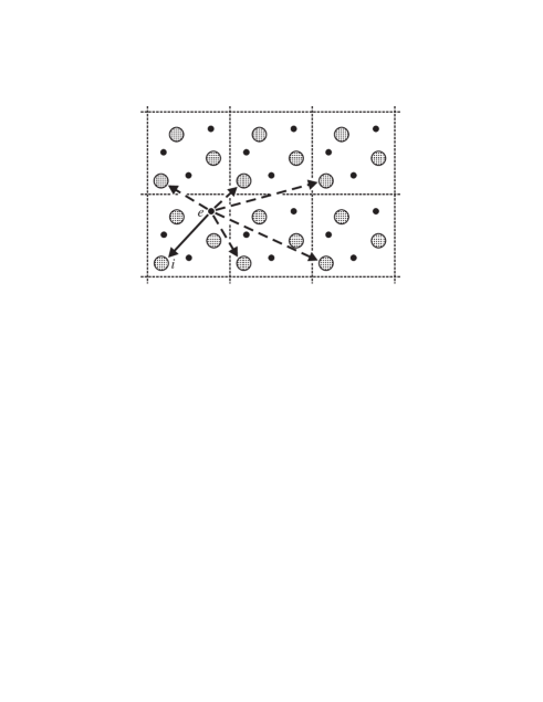
Figure 1: Sketch illustrating the interaction between an electron ($e$) and ion ($i$) both inside the basic cell (solid arrow) and with all its mirror images (dashed arrows). The ions are pictorially drawn by the large circles; and electrons, by the small ones (in fact, all the particles in our simulation were point-like).

So, we worked with a relatively small number of the equations of motion—only for particles in the basic cell. As a result, we could perform integration with a very small step and, therefore, automatically avoid the problem of close collisions without any artificial modification of the Coulomb’s potential. On the other hand, the total number of the charged particles participating in Coulomb interactions (including the mirror images) was in our calculations between 100 000 and 3 000 000. This is not less and even usually much greater than in the simulations by other researchers.

3.2 Initial Equations

As was already mentioned in Sec. 2, the ion kinetic energy in the experiments with magneto-optical traps is usually small as compared to the kinetic energy of electrons. Consequently, the ions in our simulation were assumed to move from the very beginning by the inertial (i.e., linear in time) law; while the electron dynamics was described taking into account Coulomb’s interactions not only inside the basic cell but also with infinite number of its mirror images:

$$m\,\frac{d^{2}}{dt^{2}}\,{\bf r}_{i}=\,\sum_{j=1}^{N}Ze^{2}\,\frac{{\bf R}_{j}-{\bf r}_{i}}{|{\bf R}_{j}-{\bf r}_{i}|^{3}}\,+\,\sum_{j=1,\,j\neq i}^{ZN}e^{2}\,\frac{{\bf r}_{i}-{\bf r}_{j}}{|{\bf r}_{i}-{\bf r}_{j}|^{3}}+$$

$$+\,\sum_{k=1}^{3}\>\sum_{n_{k}=-\infty,\,n_{k}\neq 0}^{+\infty}\Bigg{\{}\sum_{j=1}^{N}Ze^{2}\frac{[\,{\bf R}_{j}+L\sum_{l=1}^{3}n_{l}{\bf e}_{l}\,]-{\bf r}_{i}}{|[\,{\bf R}_{j}+L\sum_{l=1}^{3}n_{l}{\bf e}_{l}\,]-{\bf r}_{i}|^{3}}+$$

$$+\,\sum_{j=1}^{ZN}\,e^{2}\frac{{\bf r}_{i}-[\,{\bf r}_{j}+L\sum_{l=1}^{3}n_{l}{\bf e}_{l}\,]}{|{\bf r}_{i}-[\,{\bf r}_{j}+L\sum_{l=1}^{3}n_{l}{\bf e}_{l}\,]|^{3}}\Bigg{\}}\>.$$ (7)

Here, ${\bf R}_{i}\;(i=1,...,N)$ are the ion coordinates, ${\bf r}_{i}\;(i=1,...,ZN)$ are the electron coordinates, $N$ is the number of ions in the basic cell, $Z$ is the ion charge (in the calculations presented below in this article, the ions were singly charged, i.e. $Z\equiv 1$), $m$ and $e$ are the mass and absolute value of the electron charge, $L$ is the linear size of the basic cell, ${\bf e}_{l}\;(l=1,2,3)$ are the unit vectors of the Cartesian coordinate system, and subscripts $n_{k}\;(k=1,2,3)$ specify the number of the mirror cell in each direction. Let us mention that a software code actually performed summation over the mirror cells not from $-\infty$ to  $+\infty$, as in formula (7), but starting from the central (basic) cell, one shell of cells after another, until a specified criterion of convergence of the Coulomb sums is satisfied.

Yet another well-known problem in modeling the freely-expanding plasmas is a considerable variation in the spatial scale of the system (and, consequently, in the values of Coulomb’s forces) during its evolution. As a result, it becomes difficult to choose the method of numerical integration ensuring a stable accuracy for the entire solution. In our modeling, this problem was resolved by introduction of a “scalable” coordinate system, expanding in space with a mean plasma expansion velocity. In other words, size of the basic cell was taken to be increasing linearly in time:

$$L=L_{0}+u_{0}\,t$$ (8)

(which corresponds, from the physical point of view, just to the inertial motion), and the coordinates of all particles were normalized to this time-dependent scale.

The ions, moving by inertia, will be exactly at rest in such coordinates, while the electrons will move within a cell of the fixed size. When the electron crosses one of boundaries of the cell, it is assumed to appear at the opposite side, as it is usually done in the method of molecular dynamics.

At last, to get the final equations of motion for the electrons, which will be used in the simulation, all physical quantities should be reduced to the dimensionless form. Let the time-dependent unit of length $\tilde{l}\,$ be the characteristic interparticle distance, determined by the following way. The total number of particles in the basic cell equals $(Z+1)N$; so the volume per one particle will be ${L^{3}}/((Z+1)N)$. Consequently, the characteristic linear size can be determined as

$$\tilde{l}=\frac{L}{(Z+1)^{1/3}\>N^{1/3}}\>.$$ (9)

Particularly, at the initial instant of time (which from here on will be denoted by subscript 0) we get:

$$\tilde{l_{0}}=\frac{L_{0}}{(Z+1)^{1/3}\>N^{1/3}}\>.$$ (10)

The characteristic time scale $\tau$ can be formally introduced, for example, by the virial relation taken at the initial instant of time: $(1/2)\,m\,(\tilde{l_{0}}/\tau)^{\,2}\,=\,(1/2)\,Ze^{2}/\,\tilde{l_{0}}\,$, from which we obtain

$$\tau={\left(\frac{m}{Ze^{2}}\right)}^{\!1/2}\>{\tilde{l_{0}}}^{\,3/2}.$$ (11)

Within a numerical factor, this coincides with the inverse Langmuir frequency (as could be expected from the dimensionality arguments).

From here on, the quantities normalized to $\tilde{l}$ and $\tau$ will be denoted by asterisks. It can be easily shown that the physical scale $\,\tilde{l}\,$ will be a function of the dimensionless time of the form:

$$\tilde{l}=\,\tilde{l_{0}}\,(1+\,u_{0}^{*}\,t^{*})\,,$$ (12)

where

$$u_{0}^{*}=u_{0}\,\tau/L_{0}\,;$$ (13)

while a dimensionless length of the basic cell is constant:

$$L^{*}=(Z+1)^{1/3}N^{1/3}.$$ (14)

Therefore, in the variables specified above, equations of the electron motion (7) will take the form:

$${\ddot{\rm\bf r}}_{i}^{*}+\,2\,u_{0}^{*}\,(1+\,u^{*}_{0}\,t^{*})^{-1}\,{\dot{\rm\bf r}}_{i}^{*}=\,(1+\,u^{*}_{0}\,t^{*})^{-3}\,{\rm\bf F}^{*}_{i}\,,$$ (15)

where dot denotes a derivative with respect to the dimensionless time $t^{*}$, and ${\rm\bf F}^{*}_{i}$ is the total Coulomb’s force acting on $i$th electron from all other electrons and ions:

$${\rm\bf F}^{*}_{i}=\,\sum_{j=1}^{N}\frac{{\bf R}^{*}_{j}-{\bf r}^{*}_{i}}{|{\bf R}^{*}_{j}-{\bf r}^{*}_{i}|^{3}}\,+\,\frac{1}{Z}\!\sum_{j=1,\,j\neq i}^{ZN}\frac{{\bf r}^{*}_{i}-{\bf r}^{*}_{j}}{|{\bf r}^{*}_{i}-{\bf r}^{*}_{j}|^{3}}\,+$$

$$+\,\sum_{k=1}^{3}\>\sum_{n_{k}=-\infty,\,n_{k}\neq 0}^{+\infty}\Bigg{\{}\sum_{j=1}^{N}\frac{[\,{\bf R}^{*}_{j}+L^{{}^{\scriptstyle*}}\sum_{l=1}^{3}n_{l}{\bf e}_{l}\,]-{\bf r}^{*}_{i}}{|[\,{\bf R}^{*}_{j}+L^{{}^{\scriptstyle*}}\sum_{l=1}^{3}n_{l}{\bf e}_{l}\,]-{\bf r}^{*}_{i}|^{3}}\,+$$

$$+\,\frac{1}{Z}\,\sum_{j=1}^{ZN}\frac{{\bf r}^{*}_{i}-[\,{\bf r}^{*}_{j}+L^{{}^{\scriptstyle*}}\sum_{l=1}^{3}n_{l}{\bf e}_{l}\,]}{|{\bf r}^{*}_{i}-[\,{\bf r}^{*}_{j}+L^{{}^{\scriptstyle*}}\sum_{l=1}^{3}n_{l}{\bf e}_{l}\,]|^{3}}\Bigg{\}}\,.$$ (16)

As follows from equation (15), the effect of inertial plasma expansion in the “expanding” coordinate system looks like the influence of an effective dissipative force, which is proportional to the electron velocities. Therefore, temperature of the electron gas results from the balance of two effects—on the one hand, acceleration and heating of the electrons due to Coulomb’s interactions and, on the other hand, their deceleration and cooling by the above-mentioned dissipative forces.

3.3 Method of Computation

To write conveniently the subsequent formulas, let us introduce the auxiliary quantity:

$$s(t^{*})=\,(1+\,u^{*}_{0}\,t^{*})^{-1}\,.$$ (17)

Then, following the standard procedure, the second-order equation (15) can be rewritten as a set of two equations of the first order:

$${\dot{\rm\bf r}}_{i}^{*}=\,{\rm\bf v}_{i}^{*}\,,$$ (18a)

$${\dot{\rm\bf v}}_{i}^{*}=-2\,u_{0}^{*}s\,{\rm\bf v}_{i}^{*}+\,s^{3}\,{\rm\bf F}^{*}_{i}\,,$$ (18b)

which can be solved by any available method of numerical integration. We used Runge–Kutta method of the second order.

The set of equations (18a) and (18b) is solved in the region

$$-L^{*}\!/2\>\leq{(r^{*}_{i})}_{l}\>\leq L^{*}\!/2\,,\quad\mbox{where \>}i=1,...,ZN\;\,\mbox{and \;}l=1,2,3$$ (19)

(the subscript $l$ denotes the number of the Cartesian coordinate) with standard molecular-dynamic boundary conditions: a particle leaving the basic cell of simulation through one of its sides is replaced by the particle entering the cell with the same velocity through the opposite side. The initial coordinates of electrons are given by the random-number generator as a uniform statistical distribution over the region (19); and the initial velocities, as Gaussian distribution with a specified dispersion.

As was already mentioned above, an ion motion in the simulated experimental conditions can be considered as inertial; so that the normalized ion coordinates in the “expanding” reference system remain constant. At the initial instant of time, they are taken as a uniform statistical distribution over the region

$$-L^{*}\!/2\>\leq{(R^{*}_{i})}_{l}\>\leq L^{*}\!/2\,,\quad\mbox{where \>}i=1,...,N\;\,\mbox{and \;}l=1,2,3\;.$$ (20)

It is unnecessary, of course, to specify the initial velocities and to solve the equations of motion for the ions.

Finally, let us discuss in more detail how to calculate a kinetic energy of the electron motion $K$ with respect to the mean plasma flow, which is related to their temperature by formula (3). We can see here one more advantage of the introduced coordinate system: the required kinetic energy is calculated in this system just by differentiating the normalized (dimensionless) electron coordinates with respect to time; and one should not differentiate the normalization factor $\,\tilde{l}(t)\,$ itself, because its variation is associated with a kinetic energy of the plasma motion as a whole:

$$K=\,\frac{m}{2}\,\sum_{i=1}^{ZN}{\bigg{(}\frac{d}{dt}\,{\rm\bf r}_{i}\!\bigg{)}}_{\rm\!rel}^{\!2}=\,\frac{m\,{\tilde{l}}^{\,2}}{2\,{\tau}^{2}}\,\sum_{i=1}^{ZN}{\bigg{(}\frac{d}{dt^{*}}\,{\rm\bf r}^{*}_{i}\!\bigg{)}}^{\!\!2}=\,\frac{m\,{\tilde{l}}^{\,2}}{2\,{\tau}^{2}}\,\sum_{i=1}^{ZN}\,({\rm\bf v}^{*}_{i}\!)^{\,2}\,.$$ (21)

By introducing the normalization factor

$$\tilde{K}=\,\frac{m}{2}\,\frac{{\tilde{l_{0}}}^{2}}{{\tau}^{2}}\;,$$ (22)

we find that the dimensionless kinetic energy of the relative motion is given by the expression:

$$K^{*}=\,s^{-2}\sum_{i=1}^{ZN}\,({\rm\bf v}^{*}_{i}\!)^{\,2}\,.$$ (23)

Just this formula (after division by the total number of particles in the basic cell) will be used below to calculate the plasma temperature.

3.4 Particular Case of the Ideal Gas

Before presentation of the results of numerical modeling, let us discuss one particular example, which can be completely solved in analytic form and demonstrates a self-consistency of the approach used. Namely, let us consider the case of an ideal gas, when the forces of interparticle interaction ${\rm\bf F}^{*}_{i}$ disappear at all (for example, because the electric charges tend to zero). Then, equation (18b) is reduced to

$${\dot{v}}_{ik}^{*}=-2\,u_{0}^{*}s\,v_{ik}^{*}$$ (24)

(subscript $i$ denotes here the number of particle, and $k$ is the number of coordinate). After the integration of this differential equation, taking into account the particular form of function $s(t^{*})$ given by formula (17), we get:

$$v_{ik}^{*}=(v_{ik}^{*})_{{}_{\scriptstyle 0}}\,(1+\,u^{*}_{0}\,t^{*})^{-2}=(v_{ik}^{*})_{{}_{\scriptstyle 0}}\,s^{2}(t^{*})\,.$$ (25)

At last, substituting solution (25) to general expression for the kinetic energy (23), we find:

$$K^{*}=\,s^{-2}\sum_{i=1}^{ZN}\,({\rm\bf v}^{*}_{i}\!)_{0}^{\,2}\,s^{4}=\,K^{*}_{0}\>s^{2}(t^{*})\>.$$ (26)

Therefore, the electron temperature $\,T_{e}\propto K\propto K^{*}\,$ will change in time by the law:

$$T_{e}(t)\propto s^{2}(t^{*})\propto(1+\,u^{*}_{0}\,t^{*})^{-2}\propto t^{-2}\quad\mbox{at large }t\,,$$ (27)

as should be expected for the inertial expansion of the ideal monatomic gas.

3.5 Basic Parameters of the Numerical Simulation

Before presentation of the results of numerical simulation for strongly-coupled plasmas, let us describe in more detail the basic parameters used in the computation presented below in Figs. 2 and 3.

The number of particles in the basic cell: $N_{\rm tot}=(Z+1)\,N=20\,$ (i.e., 10 electrons and 10 ions). Due to the so small number of particles, we were able to perform integration with high accuracy (see below for more details) over the time interval ${\Delta}_{\rm tot}t^{*}\approx 1000$. The total number of particles taken into account in the calculation of Coulomb sums (including the mirror cells) was, on the average, a few hundred thousand (more exactly, 137 180 to 3 327 500).

In other versions of simulation, for example, when the number of particles in the basic cell was increased by an order of magnitude—up to $\,N_{\rm tot}=200$, we were enforced to decrease the interval of integration by $3{\div}4$ times; but the behavior of macroscopic plasma parameters remained qualitatively the same. When $N_{\rm tot}$ was further increased by a few more times, the reachable interval of integration became so short that it was difficult to draw reliable conclusions on the laws of evolution of the plasma parameters with time.

The step of integration and the accuracy of calculation of the Coulomb’s forces: $\Delta t^{*}=10^{-3}{\div}\,10^{-4}$ and ${\varepsilon}_{F}=10^{-3}{\div}\,10^{-4}$. These values were chosen empirically, by a series of test simulations. Starting from the above-written values, the behavior of macroscopic plasma parameters became reproducible, i.e. independent of further increase in the accuracy of computation. Let us mention that the integration step $\Delta t^{*}=10^{-3}$ was usually sufficient. However, at some “unfavorable” initial distributions of the particles, there might be a few close collisions when such integration step was too large. In these cases, it should be reduced to $10^{-4}$ and sometimes even smaller.

Velocity of the inertial plasma expansion: $u_{0}^{*}=0.1\,$. Such value of the expansion velocity at the time interval under simulation results in increasing the plasma cloud size by a few dozen times, which corresponds to the experimental conditions [11].

Root-mean-square scatter of the initial velocities of the particles: ${\sigma}_{v0}^{*}=3.0$ (in each Cartesian coordinate), i.e. initially the plasma was taken to be slightly nonideal. In some other simulations, we used greater values of ${\sigma}_{v0}^{*}$, i.e. started from a more ideal plasma state. In such cases, the initial stage of evolution of the electron temperature was close to the expected dependence $T_{e}\propto t^{-2}$. In subsequent modeling, to avoid spending a lot of time for the integration over the physically trivial interval, we preferred to start just from ${\sigma}_{v0}^{*}=3.0\,$.

3.6 Results of the Simulation

The results of our numerical simulation for the electron temperature are presented by crosses in logarithmic scale in Fig. 2. After excluding from a consideration the earliest period of time, when relaxation processes occurred, the points in the remaining time interval lie almost along a straight line, corresponding to the power law $T_{e}\propto t^{\alpha}$. The respective exponent was found to be in the range $\alpha=-(1.08{\div}1.25)$. This is quite close to the value $\alpha=-1$, following from the simple virial estimate, and is in perfect agreement with the experimental value $\alpha=-(1.1{\div}1.3)$ [11].

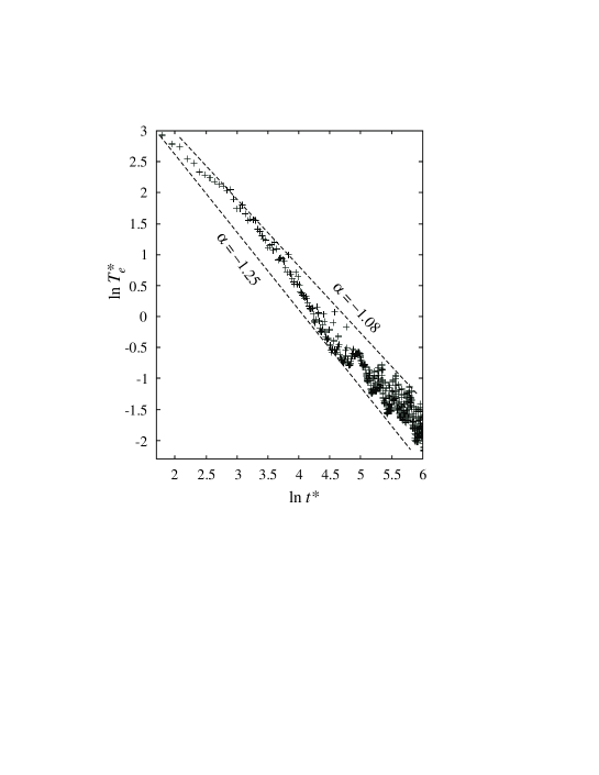
Figure 2: Electron temperature obtained by the numerical simulation as function of time in the logarithmic coordinate system. The inclined straight lines show the power-like dependences of the form $\,T_{e}\propto t^{\alpha}$; the values of $\alpha$ being presented near the respective lines.

It is reasonable to ask if the dependence obtained is really caused by the effect of virialization, discussed in Sec. 2? To answer this question, we plotted in Fig. 3 the temporal dependences of average kinetic energy and one-half the absolute value of the potential (Coulomb’s) energy in ordinary (not logarithmic) coordinates. These quantities were obtained by the method of moving average over the interval ${\Delta}_{\rm avr}t^{*}=20$ (i.e. 10 units of dimensionless time in both sides from the center). It is seen in this figure that at large time, $t^{*}\approx 500$, the curves $\overline{k}^{\,*}(t^{*})$ and $|\overline{u}^{\,*}(t^{*})|/2$ begin to coincide with a sufficiently good accuracy, about 10%. On the other hand, it is important to emphasize that the above-mentioned power law of evolution of $T_{e}$ with exponent $\alpha=-(1.1{\div}1.3)$ is established much earlier, when the virialization criterion is satisfied only on the order of magnitude. Probably, this is just the reason why $\alpha$ differs from the exact value of $-1$. This question requires a further careful study.

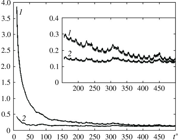
Figure 3: Temporal behavior of the average kinetic energy per one particle $\overline{k}^{\,*}$ (curve 1) and one-half the absolute value of average potential (Coulomb’s) energy $|\overline{u}^{\,*}|/2$ (curve 2).

At last, it is interesting to compare our findings with the results of paper [21], which was based on a quite complex “hybrid model” of ultracold plasmas. It involved the quasi-hydrodynamic equations for ions, description of the electron dynamics by Monte-Carlo method, as well as additional inclusion of some collisional processes by the a priori information about their cross-sections. As a result, it was in particular found that, if the three-body recombination was not included explicitly, then the electron coupling parameter ${\Gamma}_{e}$ increases infinitely with time at any initial temperature. On the other hand, if the effects of three-body recombination and subsequent inelastic collisions of electrons with the produced Rydberg atoms were included to the equations as additional terms, then the coupling parameter was stabilized in the course of time at the level ${\Gamma}_{e}\approx 0.2$ (see Fig. 3 in paper [21]).

Unfortunately, this conclusion does not agree with the results of paper [17], published almost at the same time. Its authors used a “pure” molecular-dynamic model, without any explicit inclusion of the three-body recombination, and found a stabilization of ${\Gamma}_{e}$ at the level about unity. However, it should be mentioned that only the slightly-expanding plasmas were considered. As regards our simulation, it also does not take into consideration any special corrections for the recombination and gives the asymptotic values of coupling parameter ${\Gamma}_{e}\approx 1$, i.e. in agreement with [17], also in the case of very large plasma expansion (by a few dozen times, in terms of the linear size).

Let us emphasize that, if the recombination processes are not taken into account explicitly in the equations of molecular dynamics, this does not mean that these processes are completely ignored. In fact, our model already involves their description from the first principles: as follows from a more careful analysis of the computational results, the scattering of crosses in Fig. 2 and spiky-like behavior of the curves in Fig. 3 are caused just by formation of quasi-bound states of the electrons and ions (i.e. by the onset of recombination between the charged particles). If the electron–ion pair with a sufficiently large eccentricity of the orbit is formed, then every passage of the electron in the vicinity of the ion will be associated with a sharp outburst of both kinetic energy and the absolute value of potential energy. This looks as a series of sharp equidistant peaks in macroscopic parameters of the plasma. A few series of such peaks were clearly observed in our simulations. However, consideration of this phenomenon requires a separate article, and it will not be discussed here in more detail.

4 Conclusions

1. The law of evolution of the electron temperature close to $t^{-1}$ can be explained, in the first approximation, by a simple analytical model based on the virialization of energy of the charged particles.

2. The numerical simulation from the first principles, using the scalable coordinate system and accurately taking into account Coulomb’s interactions, results in some deviation of the exponent, namely, from $-1$ to $-(1.08{\div}1.25)$, which is in perfect agreement with the experimental value.

3. Therefore, the decelerated law of decrease in the electron temperature is, first of all, a manifestation of the specific equation of state of the cold nonideal plasma rather than a result of additional heat release due to recombination.

4. It was unexpectedly found in the numerical simulation that the law of variation in the electron temperature of the form $T_{e}\propto t^{-(1.08{\div}1.25)}$ is established very quickly—when the virial relation for energies is satisfied only within a factor on the order of unity.

5. A more careful analysis of the results of our simulation reveals also some finer effects, for example, the quasi-periodic oscillations of energy caused by the formation of bound electron–ion states.

REFERENCES:

1. Fortov V.E., Khrapak A.G., Yakubov I.T. Physics of Nonideal Plasmas (Fizika neideal’noi plazmy), Fizmatlit, Moscow, 2004 (in Russian).
2. Killian T.C., Pattard T., Pohl T., Rost J.M. // Phys. Rep. 2007. V. 449. P. 77.
3. Simien C.E., Chen Y.C., Gupta P., et al. // Phys. Rev. Lett. 2004. V. 92. P. 143001.
4. Tkachev A.N., Yakovlenko S.I. // JETP Lett. 2001. V. 73. P. 66.
5. Gould P., Eyler E. // Phys. World. 2001. V. 14(3). P. 19.
6. Bergeson S., Killian T. // Phys. World. 2003. V. 16(2). P. 37.
7. Morrison J.P., Rennick C.J., Keller J.S., Grant E.R. // Phys. Rev. Lett. 2008. V. 101. P. 205005.
8. Dumin Yu.V. // J. Low Temp. Phys. 2000. V. 119. P. 377.
9. Dumin Yu.V. // Astrophys. Space Sci. 2001. V. 277. P. 139.
10. Roberts J.L., Fertig C.D., Lim M.J., Rolston S.L. // Phys. Rev. Lett. 2004. V. 92. P. 253003.
11. Fletcher R.S., Zhang X.L., Rolston S.L. // Phys. Rev. Lett. 2007. V. 99. P. 145001.
12. Lankin A.V., Norman G.E. // J. Phys. A: Math. Theor. 2009. V. 42. P. 214042.
13. Landau L.D., Lifshitz E.M. Mechanics (3rd ed.), Pergamon, Oxford, 1976.
14. Landau L.D., Lifshitz E.M. Statistical Physics, V. 1 (3rd ed.), Pergamon, Oxford, 1980.
15. Fletcher R.S., Zhang X.L., Rolston S.L. // Phys. Rev. Lett. 2006. V. 96. P. 105003.
16. Bobrov A.A., Bronin S.Ya., Zelener B.B., et al. // J. Exp. Theor. Phys. 2008. V. 107. P. 147.
17. Kuzmin S.G., O’Neil T.M. // Phys. Rev. Lett. 2002. V. 88. P. 065003.
18. Mazevet S., Collins L.A., Kress J.D. // Phys. Rev. Lett. 2002. V. 88. P. 055001.
19. Robicheaux F., Hanson J.D. // Phys. Plasm. 2003. V. 10. P. 2217.
20. Pohl T., Pattard T., Rost J.M. // Phys. Rev. Lett. 2004. V. 92. P. 155003.
21. Robicheaux F., Hanson J.D. // Phys. Rev. Lett. 2002. V. 88. P. 055002.