Phonon-mediated decoherence in triple quantum dot interferometers

Abstract

We investigate decoherence in a triple quantum dot in ring configuration in which one dot is coupled to a damped phonon mode, while the other two dots are connected to source and drain, respectively. In the absence of decoherence, single electron transport may get blocked by an electron falling into a superposition decoupled from the drain and known as dark state. Phonon-mediated decoherence affects this superposition and leads to a finite current. We study the current and its shot noise numerically within a master equation approach for the electrons and the dissipative phonon mode. A polaron transformation allows us to obtain a reduced equation for only the dot electrons which provides analytical results in agreement with numerical ones.

I Introduction

Coherently coupled quantum dots allow the experimental investigation of electron transport through delocalized orbitals and the associated coherent superpositions. The latter are visible in the charging diagram of double or triple quantum dots as broadened lines between regions in which an electron is localized in the one or the other dot. The consequence for the current-voltage characteristics is that Coulomb steps discern into multiple steps, each corresponding to an orbital that enters the voltage window.Gaudreau2006a ; Schroer2007a ; Onac2006a ; Taubert2008a When coupled quantum dots are arranged in a ring configuration as sketched in Fig. 1, electrons can proceed in two ways from the source to the drain.Gustavsson2006a ; Rogge2008a Then interference effects emerge, provided that the tunneling is coherent. For cetain phases of the tunnel matrix element, a superposition decoupled from the drain is formed such that an electron may become trapped in the interferometer.Michaelis2006a ; Emary2007b ; Busl2010a ; Busl2010b Owing to Coulomb repulsion, these so-called dark states block the electron transport. Detuning the energy of one of the dots forming the superposition resolves this blockade, but leads to temporal trapping by off-resonant tunneling to and from the detuned dot. This leads to avalanche-like transport with super-Poissonian noise.Emary2007b ; Dominguez2010a

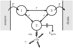
Figure 1: Triple quantum dot in ring configuration with mutual tunnel couplings $\tau$. Dots 1 and 3 possess onsite energies $\epsilon_{1,3}=0$ and are tunnel coupled to the source and the drain, respectively. Dot 2 interacts with a damped vibrational mode with frequency $\omega_{0}$, while its onsite energy can be tuned by a gate voltage such that $\epsilon_{2}=V_{\rm gate}/e$. Dot 2 has a vibrational degree of freedom, while dots 1 and 3 are rigidly attached to the contacts.

The natural enemy of interference is decoherence, i.e., the loss of the quantum mechanical phase. The common scenario for this process is that the considered system interacts with environmental degrees of freedom and, thus, becomes entangled with them. Then tracing out the environment diminishes interference and the system tends to behave classically. A frequently employed model for describing decoherence is the linear coupling of a central system to a bath of harmonic oscillators representing, e.g., phonons or photons. Magalinskii1959a ; Caldeira1983a ; Leggett1987a ; Hanggi1990a Owing to the linearity of both the bath and its coupling to the system, the former can be eliminatedFeynman1963a yielding a master equation or a path integral description of the now dissipative central system. If decoherence stems from the coupling to fermionic baths such as nuclear spins or defects, a spin bath model is more appropriate.Stamp1988a ; Shao1998a ; Prokofev2000a Electron spin decoherence is can be induced by hyperfine interaction of an electron placed in a single Yao2007a or double quantum dot, where decoherence affects spin blockade regime.Dominguez2009a

A slightly different scenario is the so-called “third-party decoherence” Stamp2006a in which a quantum system couples via a further small quantum system to a bath consisting of many degrees of freedom. A particular case is the coupling of the quantum system via a harmonic oscillator to a bath of harmonic oscillators. This system-oscillator-bath model is equivalent to a system-bath model with a spectral density peaked at the oscillator frequency,Wilhelm2004a ; Thorwart2004a ; Goorden2004a unless nonlinearities of the oscillator are taken into account.Vierheilig2009a

Here we investigate how destructive interference in a triple quantum dot interferometer is modified by the coupling to a dissipative harmonic oscillator. We focus on the regime of weak dot-lead tunneling in which a master equation description is appropriate. Nevertheless, the electron dynamics may exhibit non-Markovian effects stemming from the coupling to the oscillator. Therefore, it is technically advantageous not to eliminate the oscillator but to treat ii as part of the central system.

Our paper is organized as follows. In Sec. II we introduce the phonon-system-lead Hamiltonian and derive a quantum master equation with which we investigate in Sec. III the impact of decoherence on the current and its noise. Section IV is devoted to an effective master equation for only the dot electrons based on a polaron transformation. Some technical details of the derivation of the effective master equation and the computation of the oscillator correlation function are deferred to the appendix.

II Triple quantum dot in ring configuration

We consider three quantum dots in the ring configuration sketched in Fig. 1. The electronic part consists of three quantum dots that are mutually tunnel coupled. Since we will focus on decoherence effects stemming from the interaction with a phonon mode, we neglect the spin degree of freedom. Moreover, we restrict ourselves to the limit of strong inter-dot and intra-dot Coulomb repulsion such that only the states with zero or one excess electron on the ring are relevant. Thus, the only relevant states are the empty state $|0\rangle$ and the one-electron states $|i\rangle=c_{i}^{\dagger}|0\rangle$, where $i=1,2,3$ refers to the dot on which the electron resides and $c_{i}^{\dagger}$ is the associated electron creation operator. Then the electronic part of the Hamiltonian reads

$$H_{\text{TQD}}=\sum_{i=1}^{3}\epsilon_{i}n_{i}+\tau\sum_{i>j}(c_{i}^{\dagger}c_{j}+\text{h.c.})\,,$$ (1)

where $\tau$ is the tunnel matrix element between dots $i$ and $j$, and $n_{i}=c_{i}^{\dagger}c_{i}$ the occupation number of the dot $i$. We consider the situation in which dots 1 and 3 are degenerate and possess onsite energies $\epsilon_{1}=\epsilon_{3}=0$. By contrast dot 2, placed in one path of the interferometer, shall be tunable by a gate voltage such that $\epsilon_{2}=eV_{\text{gate}}$. In order to include the Aharonov-Bohm phase produced by a flux $\Phi$ through the ring,Aharonov1959a we multiply the operators for clockwise tunneling by $e^{i\phi}$, while counter-clockwise tunnel matrix elements acquire the factor $e^{-i\phi}$, where $\phi=2\pi\Phi/\Phi_{0}$ with the flux quantum $\Phi_{0}=h/2e$.

Dots 1 and 3 are tunnel coupled to metallic leads which is described by the Hamiltonians

$$H_{\text{leads}}= \sum_{\ell,k}\epsilon_{\ell k}c_{\ell k}^{\dagger}c_{\ell k},$$ (2)

$$H_{\text{dot-leads}}= \sum_{k}(V_{Lk}c_{Lk}^{\dagger}c_{1}+V_{Rk}c_{Rk}^{\dagger}c_{3}+\text{h.c.}),$$ (3)

where $c_{\ell k}^{\dagger}$ and $c_{\ell k}$, $\ell=L,R$, create and annihilate an electron in left and in the right lead, respectively. The tunnel matrix elements $V_{\ell k}$ enter only via their spectral density $\Gamma_{\ell}=2\pi\sum_{k}|V_{\ell k}|^{2}\delta(\epsilon-\epsilon_{\ell k})$ which we assume to be independent of the energy $\epsilon$. Then $\Gamma_{\ell}$ is the tunnel rate between lead $\ell$ and the respective dot.

II.1 Electron-phonon interaction

An electron on dot 2 interacts linearly with a localized phonon mode according to Brandes2003a

$$H_{\text{ph}}=\hbar\omega_{0}a^{\dagger}a,$$ (4)

$$V_{\text{e-ph}}=\lambda c_{2}^{\dagger}c_{2}(a^{\dagger}+a),$$ (5)

which can be interpreted as a dynamical energy shift. In turn, an electron on dot 2 entails a force on the oscillator, such that the latter acquires information about the path that an electron takes on its way from source to drain. Such “which way information” influences interference properties. Notice that we treat the coupling energy $\lambda$ as parameter despite the fact that it can be determined from microscopic considerations.Brandes2003a

Dissipation of the localized phonon mode $a$ stems from the interaction with a bosonic environment such as substrate phonons. The environment and its coupling to mode $a$ are described by the system-bath Hamiltonian

$$H_{\text{env}}= \sum_{\nu}\hbar\omega_{\nu}a_{\nu}^{\dagger}a_{\nu},$$ (6)

$$H_{D}= (a^{\dagger}+a)\sum_{\nu}\lambda_{\nu}(a_{\nu}^{\dagger}+a_{\nu}),$$ (7)

where $a_{\nu}$ and $a_{\nu}^{\dagger}$ are the creation and annihilation operators of the bath modes, while $\lambda_{\nu}$ are the coupling constants. The influence of the environment is fully determined by its spectral density $I(\omega)=\pi\sum_{\nu}|\lambda_{\nu}|^{2}\delta(\omega-\omega_{\nu})$, which we assume to be Ohmic, i.e., $I(\omega)=\gamma\omega$, where $\gamma$ denotes the effective damping rate.

II.2 Quantum master equation

In order to derive a master equation for the dissipative dynamics of the triple quantum dot and the localized mode, we start from the Liouville-von Neumann equation for the full density operator, $i\hbar\dot{R}=[H_{\text{tot}},R]$, where $H_{\text{tot}}$ is the sum of all the Hamiltonians appearing above. Using standard techniques,Blum1996a we obtain for the reduced density operator the equation of motion

$$\dot{\rho}={} -\frac{i}{\hbar}[H_{0},\rho]$$

$$-\frac{1}{\hbar^{2}}\mathop{\mathrm{Tr}}\nolimits_{\text{leads+bath}}\int_{0}^{\infty}dt[H_{V},[\tilde{H}_{V}(-t),R]]$$ (8)

$$\equiv{} \mathcal{L}\rho,$$ (9)

which can be evaluated under the factorization assumption $R\approx\rho_{\text{leads},0}\otimes\rho_{\text{bath},0}\otimes\rho$. We have defined $H_{0}=H_{\text{TQD}}+H_{\text{ph}}+V_{\text{e-ph}}$. The tilde denotes the interaction picture with respect to the Hamiltonian $H_{0}+H_{\text{\text{leads}}}+H_{\text{\text{bath}}}$, i.e., $\tilde{X}(t)=U_{0}^{\dagger}(t)XU_{0}(t)$. The coupling of the central system to the leads and the heat bath has been subsumed in the interaction Hamiltonian $H_{V}=H_{\text{dot-leads}}+H_{D}$.

We insert $H_{\text{dot-leads}}$ and $H_{D}$ and evaluate the trace of the electron and phonon reservoirs to obtain the Liouvillian Armour2002a ; Gurvitz1996a

$$\begin{split}\mathcal{L}\rho=&-\frac{i}{\hbar}[H_{0},\rho]-\frac{\Gamma_{L}}{\hbar}(2c_{1}\rho c_{1}^{\dagger}-c^{\dagger}_{1}c_{1}\rho-\rho c^{\dagger}_{1}c_{1})\\ &-\frac{\Gamma_{R}}{\hbar}(2c_{3}\rho c_{3}^{\dagger}-c^{\dagger}_{3}c_{3}\rho-\rho c^{\dagger}_{3}c_{3})\\ &+\frac{\gamma}{2}(\bar{n}+1)(2a\rho a^{\dagger}-a^{\dagger}a\rho-\rho a^{\dagger}a)\\ &+\frac{\gamma}{2}\bar{n}(2a^{\dagger}\rho a-aa^{\dagger}\rho-\rho aa^{\dagger}),\end{split}$$ (10)

where $\bar{n}=[\exp(\hbar\omega_{0}/k_{B}T)-1]^{-1}$ is the thermal occupation number of the localized mode at temperature $T$. Restricting ourselves to the limit in which all dot states lie within the voltage window, we have replaced the Fermi function of the left lead by 1 and that of the right lead by 0. Only in this limit, the dot-lead tunnel terms proportional to $\Gamma_{L,R}$ assume this simple form. Moreover, we consider the oscillator dissipation within rotating-wave approximation.Gardiner2004a

In order to obtain a current operator in the reduced Hilbert space, we start from the definition of the current as the change of the charge in the right lead $eN_{R}$. The according current operator $\mathcal{J}=(ie/\hbar)[H_{\text{tot}},N_{R}]$ still depends on lead operators. These are eliminated within the same approximations that yield the master equation (10). The result can be separated into two contributions, $\mathcal{J}^{+}$ and $\mathcal{J}^{-}$, which describe electron tunneling from the triple quantum dot to the right lead and back, respectively.on_currentoperator In the present case of unidirectional transport, $\mathcal{J}^{-}=0$, while

$$\mathcal{J}^{+}=\frac{e\Gamma_{3}}{\hbar}c_{3}^{\dagger}\rho c_{3}.$$ (11)

Then the stationary current expectation value reads

$$I=\mathop{\mathrm{Tr}}\nolimits\mathcal{J}^{+}\rho_{\infty},$$ (12)

where $\rho_{\infty}$ denotes the stationary solution of the master equation (10).

Further information about the transport process is provided by the zero-frequency noise $S$ which is essentially the rate at which the charge variance in one lead changes, i.e., $S=\lim_{t\to\infty}\langle\Delta Q_{R}^{2}\rangle/t$. It can be computed in the same way as the stationary current but with $N_{R}$ replaced by $N_{R}^{2}$. For unidirectional transport, one obtainsNovotny2004a

$$S=e\mathop{\mathrm{Tr}}\nolimits\mathcal{J}^{+}\rho_{\infty}-2e\mathop{\mathrm{Tr}}\nolimits\mathcal{J}^{+}{\hat{\mathcal{L}}}^{-1}\mathcal{J}^{+}\rho_{\infty},$$ (13)

where ${\hat{\mathcal{L}}}^{-1}$ is the pseudo-inverse of $\mathcal{L}$, whose action on $\mathcal{L}\rho_{\infty}\equiv X$ is computed by solving $\mathcal{L}X=\mathcal{J}^{+}\rho_{\infty}$ under the condition $\mathop{\mathrm{Tr}}\nolimits X=0$. Below we will always discuss the noise strength in relation to the current. This motivates the definition of the Fano factor $F=S/eI$, which assumes the value $F=1$ for a Poisson process.

For a numerical solution, we will have to truncate the Hilbert space of the localized phonon mode at some maximal phonon number $N$. Unless explicitly stated otherwise, truncation at $N=20$ ensured numerical convergence.

III Transport properties: numerical results

In order to outline the behavior of the triple dot under the influence of the dissipative phonon, we investigate numerically two situations. In the first one, all dots are in resonance, such that a dark state blocks transport. The second one is that of a strongly detuned dot 2, in which the blocking becomes imperfect. We also consider a magnetic flux through the triple quantum dot for ascertaining interference.

III.1 All dots in resonance

Figure 2: Current at zero detuning, $\epsilon_{2}=0$, as a function of the scaled magnetic flux $\phi$ for two values of the phonon damping strengths $\gamma$ compared to the current in the absence of the phonon ($\lambda=0$). The dot-lead tunneling rate is $\Gamma=0.1\omega_{0}$. In the non-interacting case, the current drops to zero at semi-integer values of the quantum flux. The Aharonov-Bohm amplitude is reduced by the phonon-mediated decoherence of the dark state.

For a small gate voltage such that $|\epsilon_{2}|\ll\tau$ all three dots are near resonance, and therefore interference is important. For the present configuration in which all three inter-dot tunnel couplings are equal, it has been shown that for $\epsilon_{2}=0$ an electron is trapped in the superpositionMichaelis2006a ; Emary2007b

$$|\Psi_{\text{dark}}\rangle=\frac{1}{\sqrt{2}}(|1\rangle-|2\rangle).$$ (14)

Obviously, it is orthogonal to state $|3\rangle$ and, thus, is decoupled from the drain. This implies that once an electron populates state (14), it cannot leave the triple dot. Since Coulomb repulsion inhibits further electrons from entering the dots, the current vanishes. At zero flux, $\phi=0$, the two paths $|1\rangle\rightarrow|3\rangle$ and $|1\rangle\rightarrow|2\rangle\rightarrow|3\rangle$ interfere destructively at the drain.Michaelis2006a ; Emary2007b If $\phi$ is changed, a finite current flows, unless $\phi$ assumes a semi-integer value,Emary2007b ; Busl2010a as is visible from the Aharonov-Bohm oscillations depicted in Fig. 2. Figure 2 also shows that when coupling dot 2 to the oscillator, Aharonov-Bohm oscillations fade out with increasing dissipation strength $\gamma$, which is a signature for the influence of decoherence. Moreover, it can be seen that this fading can be read off faithfully at $\phi=0$ and, thus, henceforth we restrict ourselves to this value.

Figure 3: Current as a function of the detuning $\epsilon_{2}$ for various values of the electron-phonon coupling $\lambda$. The inter-dot tunneling and the dot-lead tunneling rate are $\tau=0.01\hbar\omega_{0}$ and $\Gamma=0.1\omega_{0}$, respectively, while the dissipation strength is $\gamma=0.05\omega_{0}$. The temperatures are (a) $T=0$ and (b) $T=1.5\hbar\omega_{0}/k_{B}$. Insets: enlargement of the region near $\epsilon_{2}=0$ demonstrating a shift of the current minimum with increasing electron-phonon coupling.

The insets of Fig. 3 show the current as a function of the detuning for various electron-phonon coupling strengths $\lambda$ and two different temperatures for small detuning. An interesting observation is that with increasing electron phonon coupling (see insets of Fig. 3), the minimal current not only grows, but also is shifted from $\epsilon_{2}=0$ to the value $\epsilon_{2}=\lambda^{2}/\hbar\omega_{0}$. This shift can be obtained by a polaron transformation, as we will detail in Sec. IV. This motivates us to henceforth plot the current as a function of the renormalized detuning $\epsilon=\epsilon_{2}-\lambda^{2}/\hbar\omega_{0}$.

Figure 4: Current and Fano factor as a function of the electron-phonon coupling for the dark state, i.e., for the detuning $\epsilon=\epsilon_{2}-\lambda^{2}/\hbar\omega_{0}=0$, at zero temperature and two values of the dissipation strength $\gamma$. All other parameters are as in Fig. 3a. The dotted lines mark the results obtained with the reduced master equation (24).

Figure 5: Current as a function of the temperature for electron-phonon coupling $\lambda=0.15\hbar\omega_{0}$ and detuning $\epsilon=\epsilon_{2}-\lambda^{2}/\hbar\omega_{0}=0$, corresponding to the dark state. The dotted lines are obtained with the reduced master equation (24) for the dot electrons. All other parameters are as in Fig. 3.

Figures 4a and 5 show the current as a function of the electron-phonon coupling and the temperature, respectively, for a detuning $\epsilon=0$ which corresponds to the dark state. Both plots confirm that the current blockade is resolved with increasing electron-phonon coupling and temperature, underlining the growing importance of decoherence. The current saturates at the value $I_{D}\approx 0.02e\Gamma/\hbar$, as a function of the electron-phonon coupling $\lambda$; see Fig. 5a. A similar behavior has been found for an interferometer that consists of two quantum dots.Marquardt2003a Figures 4b depicts the associated current noise in terms of the Fano factor. Starting at the super-Poissonian value $F=3$, the Fano factor reduces towards $F\approx 1$, indicating a transition from avalanche-like transport to a Poisson process.

III.2 Dot 2 far from resonance

When dot 2 is strongly detuned, i.e., for $|\epsilon_{2}|\gg\tau$, tunneling from and to this dot becomes off-resonant. Then the direct path from dot 1 to dot 3 is much more likely than the detour via dot 2. Then without the oscillator, we expect interference effects to play a minor role. Nevertheless, electrons may be trapped in dot 2 such that the current flow is interrupted until the trapped electron tunnels off-resonantly to dot 3 and transport is restored. Consequently, the electron transport becomes bunched.Dominguez2010a The current plotted in Fig. 3 demonstrates that this scenario needs to be refined when the electron on dot 2 couples to a vibrational mode, because then temporal electron trapping can be caused also by emission and absorption of phonons. This leads to dips and peaks in the current whenever $\epsilon_{2}$ is detuned by roughly an integer multiple of $\hbar\omega_{0}$. For finite temperature and negative detuning (Fig. 3b for $\epsilon_{2}<0$), the dips are caused by the predominating phonon emission, while those for positive detuning are due to the a more frequent absorption. The different size of the peaks and dips for positive and negative values of $\epsilon$ (Fig. 3b) stems from spontaneous processes which render emission more likely than absorption. In the zero temperature limit (Fig. 3a), phonon absorption no longer occurs and consequently, the dips at positive detuning vanish. Then small peaks emerge, which correspond to the relaxation of electrons that temporally populate in dot 2.

IV Elimination of the dissipative phonon

In order to obtain a reduced master equation for the triple quantum dot, we eliminate the phonon via a polaron transformation under a weak-coupling assumption.Brandes1999a ; Brandes2003a This converts the electron-phonon coupling into a renormalized inter-dot tunneling and additional dissipative terms. In order to keep decoherence effects stemming from the phonon-bath coupling, we have to apply this transformation also to those terms of the master equation (10) that describe phonon dissipation.

IV.1 Polaron transformation

We start with the unitary transformationMahan1990a ; Brandes1999a $O\to\bar{O}=SOS^{\dagger}$ of the master equation (10), where

$$S=\exp\left[\frac{\lambda}{\hbar\omega_{0}}n_{2}(a^{\dagger}-a)\right].$$ (15)

This corresponds to the replacements

$$a\to{} a-\frac{\lambda}{\hbar\omega_{0}}n_{2},$$ (16)

$$c_{2}\to{} c_{2}X^{\dagger}$$ (17)

with the phonon displacement operator

$$X=\exp\Big{[}\frac{\lambda}{\hbar\omega_{0}}(a^{\dagger}-a)\Big{]}.$$ (18)

Notice that all lead and bath operators remain unchanged. The Hamiltonian $H_{0}$ of the dot electrons and the phonon then reads

$$\bar{H}_{0}=\epsilon\widehat{n}_{2}+\tau(c_{1}^{\dagger}c_{3}+c_{2}^{\dagger}c_{3}X+c_{1}^{\dagger}c_{2}X^{\dagger}+\text{h.c.})+\hbar\omega_{0}a^{\dagger}a,$$ (19)

where $\epsilon=\epsilon_{2}-\lambda^{2}/\hbar\omega_{0}$ denotes the effective detuning.

The form (19) of the system Hamiltonian allows us to eliminate the phonon within second-order perturbation theory in the interdot tunneling. Then we obtain a master equation for the electron operators which still depends on electron-oscillator correlations. Next, the phonon is traced out under the assumption that the polaron transformation captures most of these correlations, such that the density operators in the polaron picture factorizes, $\rho=\rho_{e}\otimes\rho_{\text{ph}}$. A similar route has been already taken in Refs. Brandes1999a, ; Brandes2003a, ; it is equivalent to the non-interacting blip approximation common in quantum dissipation.Dekker1987a ; Dekker1987b ; Morillo1993a Here we only discuss the resulting master equation, while details of the derivation are provided in Appendix A.

The resulting quantum master equation contains the effective dot Hamiltonian

$$H_{\text{TQD,eff}}=\epsilon n_{2}+\tau(c_{1}^{\dagger}c_{3}+\text{h.c.})+\bar{\tau}(c_{2}^{\dagger}c_{3}+c_{1}^{\dagger}c_{2}+\text{h.c.}),$$ (20)

where the electron tunneling between dot 2 and the two other quantum dots is renormalized according to

$$\tau\to\bar{\tau}=\tau\langle X\rangle=\tau\exp\Big{\{}-\Big{|}\frac{\lambda}{\omega_{0}}\Big{|}^{2}\coth\Big{(}\frac{\hbar\omega_{0}}{2k_{B}T}\Big{)}\Big{\}}.$$ (21)

Besides this renormalization, two additional Liouvillians emerge. The first one describes decoherence of the dark state, leading to a small residual current. It is directly obtained by the replacement (16) in the last two terms of the master equation (10) and reads

$$\mathcal{L}_{\text{dec}}\rho_{e}=\frac{\gamma}{2}(1+2\bar{n})\Big{(}\frac{\lambda}{\hbar\omega_{0}}\Big{)}^{2}(2n_{2}\rho_{e}n_{2}-n_{2}\rho_{e}-\rho_{e}n_{2}),$$ (22)

where we have used the operator relation $n_{2}^{2}=n_{2}$. We will further analyze the corresponding decoherence mechanism in Sec. IV.2. The second Liouvillian stems from the double commutator in the Bloch-Redfield master equation (34) and describes incoherent tunneling between the quantum dots,

$$\begin{split}\mathcal{L}_{\text{ict}}\rho_{e}=&-\Big{(}\frac{\tau}{\hbar}\Big{)}^{2}\left\{\Big{(}C_{-\epsilon}\left(n_{1}+n_{3}\right)+2n_{2}C_{\epsilon}\Big{)}\rho_{e}+\text{h.c.}\right\}\\ &+2\Big{(}\frac{\tau}{\hbar}\Big{)}^{2}\big{\{}C_{-\epsilon}^{\prime}c_{2}^{\dagger}c_{3}\rho_{e}c_{3}^{\dagger}c_{2}+C_{-\epsilon}^{\prime}c_{2}^{\dagger}c_{1}\rho_{e}c_{1}^{\dagger}c_{2}\\ &+C_{\epsilon}^{\prime}c_{1}^{\dagger}c_{2}\rho_{e}c_{2}^{\dagger}c_{1}+C_{\epsilon}^{\prime}c_{3}^{\dagger}c_{2}\rho_{e}c_{2}^{\dagger}c_{3}\Big{\}},\end{split}$$ (23)

where $C_{\epsilon}\equiv C_{\epsilon}^{\prime}+iC_{\epsilon}^{\prime\prime}$ denotes the phonon correlation function in Laplace space, derived in Appendix B. This incoherent inter-dot tunneling is responsible for the current dips and peaks at the resonances $\epsilon=n\hbar\omega_{0}$ observed in Figs. 3 and 6. It occurs with the rates $2(\tau/\hbar)^{2}C_{\epsilon}^{\prime}$ (between dots 1 and 3) and $2(\tau/\hbar)^{2}C_{-\epsilon}^{\prime}$ (between dot 2 and dots 1,3), respectively, which is in accordance with $P(E)$-theory.Ingold1992a ; Brandes2005a

In summary, the effective master equation for the triple quantum dot under the influence of a dissipative phonon and with the coupling to the leads reads

$$\begin{split}\dot{\rho}_{e}=&-\frac{i}{\hbar}[H_{\text{TQD,eff}},\rho_{e}]+\mathcal{L}_{\text{dec}}\rho_{e}+\mathcal{L}_{\text{ict}}\rho_{e}\\ &-\frac{\Gamma_{L}}{\hbar}(2c_{1}\rho_{e}c_{1}^{\dagger}-c^{\dagger}_{1}c_{1}\rho_{e}-\rho_{e}c^{\dagger}_{1}c_{1})\\ &-\frac{\Gamma_{R}}{\hbar}(2c_{3}\rho_{e}c_{3}^{\dagger}-c^{\dagger}_{3}c_{3}\rho_{e}-\rho_{e}c^{\dagger}_{3}c_{3}).\end{split}$$ (24)

Numerical calculations provide evidence that $\mathcal{L}_{\text{ict}}$ is not relevant for the bahavior of the dark state (see Fig. 4). Thus, close to $\epsilon=0$, we can neglect $\mathcal{L}_{\text{ict}}$ in the master equation (24), and then we obtain to lowest order in $\tau$ the stationary current

$$I_{D}\approx\frac{4\Gamma\left(4g_{1}(\tau^{2}-\bar{\tau}^{2}\right)^{2}+g_{1}g_{2}\tau^{2}\Gamma_{D}+g_{2}\bar{\tau}^{2}\Gamma\Gamma_{D}}{\Gamma(2\Gamma+3\Gamma_{D})(4g_{1}\bar{\tau}^{2}+g_{2}\Gamma\Gamma_{D})+4\tau^{2}\left(2\Gamma^{3}+7\Gamma^{2}\Gamma_{D}+12\Gamma\Gamma_{D}^{2}+8\Gamma_{D}^{3}\right)},$$ (25)

with $g_{1}=\Gamma+2\Gamma_{D}$, $g_{2}=\Gamma+\Gamma_{D}$, and the effective dissipation rate $\Gamma_{D}=(\frac{1}{2}+\bar{n})\gamma(\lambda/\hbar\omega_{0})^{2}$. The validity of this result close to the dark state is investigated with Figs. 4 and 5. The agreement is rather good for any coupling constant $\lambda$ and temperature. The according result for the Fano factor also fits well (see Fig. 4b). A comparison in a broad range of detunings, shown in Fig. 6, demonstrates that the approximation is globally valid.

Figure 6: Comparison of the results with the full quantum master equation (10) and those of the effective master equation (24) for $\lambda=0.1\hbar\omega_{0}$, $\gamma=0.05\omega_{0}$, $\tau=0.01\hbar\omega_{0}$ and $\Gamma=0.1\omega_{0}$. The temperature is(a) $T=0$ and (b) $T=1.5\hbar\omega_{0}/k_{B}$.

IV.2 Decoherence mechanism

A physical picture of the electron decoherence can be developed by considering the influence of the phonon on the dark state (14). This reasoning will also yield the associated decoherence rate of the effective Liouvillian (22).

Let us assume that the electron resides in the dark state $|\Psi_{\text{dark}}\rangle\propto|1\rangle-|2\rangle$. Its time evolution under the influence of the phonon is determined by the interaction-picture Hamiltonian

$$H_{I}(t)=\lambda n_{2}(t)(a^{\dagger}e^{i\omega_{0}t}+ae^{-i\omega_{0}t}).$$ (26)

Since the electron dynamics is much slower than the oscillator, the number operator $n_{2}$ is essentially time-independent. Then the time ordering in the corresponding time-evolution operator

$$U(t)=T_{\leftarrow}\exp\Big{[}-\frac{i}{\hbar}\int_{0}^{t}ds\,H_{I}(s)\Big{]}$$ (27)

can be evaluated by employing the commutation relationBreuer2003a

$$[H_{I}(t),H_{I}(t^{\prime})]=2i\lambda^{2}n_{2}\sin[\omega_{0}(t-t^{\prime})]$$ (28)

from which we obtain the propagator

$$U(t)=\exp\left[-\frac{1}{2}\int_{0}^{t}ds\,ds^{\prime}[H_{I}(s),H_{I}(s^{\prime})]\theta(s-s^{\prime})\right]V(t).$$ (29)

The operator $V(t)=\exp\{n_{2}[a^{\dagger}\alpha(t)-a\alpha(t)^{*}]\}$ describes an oscillator displacement by

$$\alpha(t)=\frac{\lambda}{\hbar\omega_{0}}(1-e^{i\omega_{0}t}),$$ (30)

while the integral of the commutator in Eq. (27) is a mere phasefactor which is not relevant for the subsequent discussion and will be ignored. Thus, the dark state evolves according to

$$U(t)|\Psi_{\text{dark}}\rangle=\frac{1}{\sqrt{2}}\big{(}|1\rangle|0\rangle_{\text{ph}}-|2\rangle|\alpha(t)\rangle_{\text{ph}}\big{)},$$ (31)

which means that the oscillator turns into a cat state, i.e., a superposition of two coherent states. The coherence of such a state is known to decay with the rate Caldeira1985a ; Walls1985a $\Gamma_{D}(t)=(\gamma/2)(1+2\bar{n})|\alpha(t)|^{2}$. For weak oscillator damping, $\gamma\ll\omega_{0}$, we can replace the rate by its time-average

$$\Gamma_{D}=\frac{\gamma}{2}(1+2\bar{n})\bigg{|}\frac{\lambda}{\hbar\omega_{0}}\bigg{|}^{2}.$$ (32)

Notice that we do not trace out the electrons, but consider the coherence of the electron-phonon compound.

Since each of the two involved phonon states is linked to a particular electron state, we can attribute this decoherence process also to the electrons. Then we can conclude that the electron coherence also decays with the rate (32), which complies with the actual rate in the effective Liouvillian Eq. (22). Thus, the phonon elimination described above is such that the decoherence of an oscillator cat state directly turns into decoherence of the dark state.

For larger inter-dot tunneling, $\tau\gtrsim\hbar\omega_{0}$, the interaction-picture operator $n_{2}(t)$ can no longer be considered time-independent, such that our reasoning has to be modified. Moreover, if we would use a model in which also dot 1 couples to the phonon, the dark electron state and the phonon state would factorize and be $\propto(|1\rangle-|2\rangle)|\alpha(t)\rangle$. Then no phonon-induced decoherence would take place and, consequently, the dark state would continue to block the electron transport.

V Conclusions

We have investigated decoherence effects in a triple quantum dot interferometer the stemming from the coupling to a single dissipative bosonic mode. In our model, the dots are arranged in a symmetric ring configuration in which two dots couple to source and drain, while the third dot interacts with a dissipative harmonic oscillator. In the absence of the oscillator, a strong detuning of the third dot leads to electron trapping and bunching. When all dots are close to resonance, by contrast, interference effects dominate. In particular, ideal destructive interference may occur, such that the current vanishes completely, even when all electronic energy levels lie within the voltage window.

It turned out that the oscillator entails two effects: First, the current minimum is found at a shifted detuning and, second, destructive interference is no longer perfect, such that always a finite current emerges. This suspension of destructive interference is also visible in the current noise measured in terms of the Fano factor. When the residual current is very small, i.e., for small decoherence, the associated shot noise is enhanced, while transport becomes almost Poissonian with stronger decoherence.

A qualitative understanding of these effects has been achieved by an analytical approximation after a polaron transformation leading to a reduced master equation for only the dot electrons. Within a standard treatment similar to the non-interacting blip approximation, we have obtained an effective master equation for the electron transport. Then it became possible to analytically obtain the current from the resulting master equation also close to destructive interference. The results agree well with the full numerical results, provided that the oscillator frequency is sufficiently large and the intra-dot tunneling is small. In turn, we can conclude that our reduced master equation faithfully describes transport effects entailed by a dissipative mode. Moreover, this picture provide evidence that the decoherence of an oscillator cat state directly turns into decoherence of the dark state.

In summary, our results underline the impact of already one phonon mode on quantum dot interferometers. With our reduced master equation for the quantum dot electrons, we have put forward a method for describing such systems efficiently after eliminating the oscillator. Such a method is in particular welcome when the oscillator is only weakly damped, since then an explicit treatment requires taking quite a few oscillator states into account.

Appendix A Effective master equation

In this appendix we provide some details of the derivation of the effective master equation (24) starting with the polaron-transformed electron-phonon Hamiltonian (19). We treat all terms that couple dot 2 to the phonon within second order perturbation theory, which means that we separate the electron-phonon Hamiltonian as $H_{\text{TQD,eff}}+H_{Y}$, where $H_{\text{TQD,eff}}$ is defined in Eq. (20) and

$$H_{Y}(t)=\tau(c_{2}^{\dagger}c_{3}Y_{t}+c_{1}^{\dagger}c_{2}Y_{t}^{\dagger}+\text{h.c.}).$$ (33)

The latter Hamiltonian will be treated within Bloch-Redfield approximation. The phonon part of the interaction, $Y=X-\langle X\rangle_{\text{eq}}$, has been defined such that $\langle H_{Y}\rangle_{\text{eq}}$ vanishes. Then within the usual Born approximation,Blum1996a we obtain in the interaction picture the master equation

$$\begin{split}\frac{d}{dt}\tilde{\rho}(t)=&-\frac{1}{\hbar^{2}}\int_{0}^{t}ds\big{[}\tilde{H}_{Y}(t),\big{[}\tilde{H}_{Y}(s),\tilde{\rho}(s)\big{]}\big{]},\end{split}$$ (34)

where the contribution of first order in the perturbation $H_{Y}$ vanishes owing to $\langle H_{Y}\rangle_{\text{eq}}=0$. A simplification of the master equation (34) comes from the fact that its right-hand side is already of second order in the inter-dot tunneling $\tau$, while higher orders are neglected. It is therefore sufficient to depricate in the interaction-picture representation of $H_{Y}$ the tunneling terms in $H_{\text{TQD,eff}}$, such that the corresponding unperturbed propagator reads $U_{0}^{\prime}=\exp(-i\epsilon n_{2}t/\hbar)$.

If the electron-phonon interaction is much smaller than the phonon energy, $\lambda\ll\hbar\omega_{0}$, the correlation between these two subsystems is by and large captured by the polaron transformation. Thus, in the polaron picture, we can evaluate the master equation under the factorization assumption $\tilde{\rho}(t)\approx\rho^{0}_{\text{ph}}\text{Tr}_{\text{ph}}\tilde{\rho}(t^{\prime})$. This corresponds to a non-interacting blip approximation Dekker1987a ; Dekker1987b ; Morillo1993a for a dissipative quantum system and has been used also to eliminate a single dissipative phonon in the context of both quantum transport Brandes2003a ; Brandes1999a and quantum dissipation.Nesi2007a

Within Born approximation, it is consistent to replace in the master equation (34) the time arguments of the density matrix by the final time $t$. When finally tracing out the phonon, we obtain expectation values of the type

$$c^{\dagger}_{i}c_{j}(t)\rho(t)c^{\dagger}_{i}c_{j}(s)\langle X^{\dagger}_{t}X_{s}\rangle,$$ (35)

$$c^{\dagger}_{i}c_{j}(t)\rho(t)c^{\dagger}_{i}c_{j}(s)\langle X_{t}X_{s}\rangle,$$ (36)

$$c^{\dagger}_{i}c_{2}(t)\rho(t)c^{\dagger}_{2}c_{j}(s)\langle X^{\dagger}_{t}X_{s}\rangle.$$ (37)

Terms of the type (35) give rise to the additional Liouvillian (23). The two following terms are negligible for different reasons. The term (36) depends on the time $t+s$ and, thus, is rapidly oscillating. Therefore it can be neglected within a rotating-wave approximation. Finally, terms of the type (37) come in pairs with opposite time-ordering and opposite sign. Therefore their net contribution is proportional to a commutator and, thus, is of the order $\tau$, i.e., one order beyond what is considered in the master equation (34).

Appendix B Correlation function

The effective Liouvillian derived in Appendix A contains averages over one and two phonon displacement operators. We calculate them using the quantum regression theorem which is valid within Markov approximation. Breuer2003a The renormalization of the coherent tunneling stems from averages of the type

$$c_{i}^{\dagger}c_{j}\langle X_{t}\rangle =c_{i}^{\dagger}c_{j}\text{Tr}_{\text{ph}}\left\{X\rho_{\text{ph}}(t)\right\}$$

$$=c_{i}^{\dagger}c_{j}\text{Tr}_{\text{ph}}\left\{X\rho_{\text{ph,eq}}\right\}$$

$$=c_{i}^{\dagger}c_{j}\exp\Big{\{}-\Big{|}\frac{\lambda}{\omega_{0}}\Big{|}^{2}\coth\Big{(}\frac{\hbar\omega_{0}}{2k_{B}T}\Big{)}\Big{\}},$$ (38)

with the equilibrium phonon density matrix

$$\rho_{\text{ph,eq}}=\frac{1}{Z}\exp(-\hbar\omega_{0}a^{\dagger}a/k_{B}T),$$ (39)

and the partition sum $Z=[1-\exp(-\hbar\omega_{0}/k_{B}T)]^{-1}$.

Using once more the quantum regression theorem, we write the correlation function as

$$C(t)=\langle X^{\dagger}(0)X(t)\rangle_{\text{eq}}=\mathop{\mathrm{Tr}}\nolimits\{X^{\dagger}(0)X_{H}(t)\rho_{\text{ph,eq}}\},$$ (40)

i.e., with a Heisenberg operator that fulfills the equation of motion $\dot{a}_{H}=-(i\omega_{0}+\gamma/2)a_{H}$. From its solution

$$a_{H}=ae^{-(i\omega_{0}+\gamma/2)t}$$ (41)

follows the displacement operator in the interaction picture,

$$X_{t}\equiv X(t)=\exp\left[\frac{\lambda}{\omega_{0}}\left(a^{\dagger}e^{(i\omega_{0}-\gamma/2)t}-\text{h.c.}\right)\right].$$ (42)

Inserting this operator and $\rho_{\text{ph,eq}}$ into the correlation function (40) yields

$$\begin{split}C(t)=&\exp\bigg{[}\Big{|}\frac{\lambda}{\omega_{0}}\Big{|}^{2}\bigg{\{}ie^{-\gamma/2t}\sin(\omega_{0}t)+\coth\Big{(}\frac{\hbar\omega_{0}}{2k_{B}T}\Big{)}\\ &\times\left(1+e^{-\gamma t}-2e^{-\gamma/2t}\cos(\omega_{0}t)\right)\bigg{\}}\bigg{]}.\end{split}$$ (43)

For computing the coefficients of the master equation, we need this correlation function in Laplace space, evaluated at $z=0$, defined as

$$C_{\epsilon}=\lim_{z\rightarrow 0}\int_{0}^{\infty}dt\,e^{-(z+i\epsilon)t/\hbar}C(t)\equiv C_{\epsilon}^{\prime}+iC_{\epsilon}^{\prime\prime}.$$ (44)

References

- (1) L. Gaudreau et al., Phys. Rev. Lett. 97, 036807 (2006).
- (2) D. Schröer et al., Phys. Rev. B 76, 075306 (2007).
- (3) E. Onac et al., Phys. Rev. Lett. 96, 176601 (2006).
- (4) D. Taubert et al., Phys. Rev. Lett. 100, 176805 (2008).
- (5) S. Gustavsson et al., Phys. Rev. Lett. 96, 076605 (2006).
- (6) M. C. Rogge and R. J. Haug, Phys. Rev. B 77, 193306 (2008).
- (7) B. Michaelis, C. Emary, and C. W. J. Beenakker, Europhys. Lett. 73, 677 (2006).
- (8) C. Emary, Phys. Rev. B 76, 245319 (2007).
- (9) M. Busl, R. Sánchez, and G. Platero, Phys. Rev. B 81, 121306(R) (2010).
- (10) M. Busl, R. Sánchez, and G. Platero, Physica E 42, 830 (2010).
- (11) F. Domínguez, G. Platero, and S. Kohler, Chem. Phys. 375, 284 (2010).
- (12) V. B. Magalinskiĭ, Zh. Eksp. Teor. Fiz. 36, 1942 (1959), [Sov. Phys. JETP 9, 1381 (1959)].
- (13) A. O. Caldeira and A. L. Leggett, Ann. Phys. (N.Y.) 149, 374 (1983).
- (14) A. J. Leggett et al., Rev. Mod. Phys. 59, 1 (1987).
- (15) P. Hänggi, P. Talkner, and M. Borkovec, Rev. Mod. Phys. 62, 251 (1990).
- (16) R. P. Feynman, R. B. Leighton, and M. Sands, The Feynman Lectures on Physics (Addison Wesley, Reading MA, 1963), Vol. 1, Chap. 46.
- (17) P. C. E. Stamp, Phys. Rev. Lett. 61, 2905 (1988).
- (18) J. Shao and P. Hänggi, Phys. Rev. Lett. 81, 5710 (1998).
- (19) N. V. Prokof’ev and P. C. E. Stamp, Rep. Prog. Phys. 63, 669 (2000).
- (20) W. Yao, R.-B. Liu, and L. J. Sham, Phys. Rev. Lett. 98, 077602 (2007).
- (21) F. Domínguez and G. Platero, Phys. Rev. B 80, 201301 (2009).
- (22) P. C. E. Stamp, Stud. Hist. Phil. Mod. Phys. 37, 467 (2006).
- (23) F. K. Wilhelm, S. Kleff, and J. von Delft, Chem. Phys. 296, 345 (2004).
- (24) M. Thorwart, E. Paladino, and M. Grifoni, Chem. Phys. 296, 333 (2004).
- (25) M. C. Goorden, M. Thorwart, and M. Grifoni, Phys. Rev. Lett. 93, 267005 (2004).
- (26) C. Vierheilig, J. Hausinger, and M. Grifoni, Phys. Rev. A 80, 069901 (2009).
- (27) Y. Aharonov and D. Bohm, Phys. Rev. 115, 485 (1959).
- (28) T. Brandes and N. Lambert, Phys. Rev. B 67, 125323 (2003).
- (29) K. Blum, Density Matrix Theory and Applications, 2nd ed. (Springer, New York, 1996).
- (30) A. D. Armour and A. MacKinnon, Phys. Rev. B 66, 035333 (2002).
- (31) S. A. Gurvitz and Ya. S. Prager, Phys. Rev. B 53, 15932 (1996).
- (32) C. W. Gardiner and P. Zoller, Quantum Noise, 3rd ed. (Springer, Berlin and Heidelberg, 2004).
- (33) A formal distinction of the incoming and the outgoing current can be achieved by introducing before the lead elimination a counting variable for the right lead, see Ref. Kaiser2007a, .
- (34) F. J. Kaiser and S. Kohler, Ann. Phys. (Leipzig) 16, 702 (2007).
- (35) T. Novotný, A. Donarini, C. Flindt, and A.-P. Jauho, Phys. Rev. Lett. 92, 248302 (2004).
- (36) F. Marquardt and C. Bruder, Phys. Rev. B 68, 195305 (2003).
- (37) T. Brandes and B. Kramer, Phys. Rev. Lett. 83, 3021 (1999).
- (38) G. D. Mahan, Many-Particle Physics, 2nd ed. (Plenum Press, New York, 1990).
- (39) H. Dekker, Phys. Rev. A 35, 1436 (1987).
- (40) H. Dekker, Physica A 141, 570 (1987).
- (41) M. Morillo and R. I. Cukier, J. Chem. Phys. 98, 4548 (1993).
- (42) T. Brandes, Phys. Rep. 408, 315 (2005).
- (43) G.-L. Ingold and Yu. V. Nazarov, in Single Charge Tunneling, Vol. 294 of NATO ASI Series B (Plenum, New York, 1992), pp. 21–107.
- (44) H.-P. Breuer and F. Petruccione, Theory of open quantum systems (Oxford University Press, Oxford, 2003).
- (45) A. O. Caldeira and A. J. Leggett, Phys. Rev. A 31, 1059 (1985).
- (46) D. F. Walls and G. J. Milburn, Phys. Rev. A 31, 2403 (1985).
- (47) F. Nesi, M. Grifoni, and E. Paladino, New. J. Phys. 9, 316 (2007).