Abstract

In this draft photometry and astrometry is presented from the Herschel Space Observatory (HSO). This spacecraft orbits the second Lagrangian point (L2) of the Sun – Earth system, yielding a mean distance of a million miles ($\approx 1.5$ million kms) for HSO. From such a distance, HSO is observable as a $17-23$ magnitude object moving relatively fast (apparently several arcseconds in a minute) and the actual observed brightness highly depends on the spatial orientation of the spacecraft. This draft describes briefly how observations from this observatory and the subsequent data reductions have been carried out. Our conclusion is really reassuring, namely the brightness variations of HSO are in accordance with the publicly available reported logs and target coordinates of this spacecraft.

1 Introduction

The Herschel Space Observatory (hereafter HSO or simply Herschel) is a far-infrared and submillimetre observatory of the European Space Agency (ESA), successfully launched on May 14, 2009 (Pilbratt et al., 2010). Herschel orbits the second Lagrangian point of the Sun – Earth system, that is apparently on the direction opposite to the Sun. The mean height of the orbit is approximately $1.5$ million kms, while the semi-amplitude of the actual motion is about the half of this value.

HSO is equipped with three on-board scientific instruments: the Photodetector Array Camera and Spectrometer (PACS, Poglitsch et al., 2010), the Spectral and Photometric Imaging Receiver (SPIRE, Griffin et al., 2010) and the Herschel-Heterodyne Instrument for the Far-Infrared (HIFI, de Graauw et al., 2010). Herschel observes a typical target from a dozen of minutes up to several hours. The list of observed targets, the utilized instruments and other information can be found on the public web page of HSO. Since the solar panels and other stuff mounted on the exterior of the spacecraft reflects the sunlight efficiently, one can expect a considerably good detectability of the spacecraft. However, due to the sharp terminations of (some of) the external devices (see any photographs of models of the observatory itself), the amount of reflected light starkly depends on the spatial orientation of the spacecraft. Indeed, the apparent visual brightness of the spacecraft can vary in a range of several magnitudes, yielding all values from the complete non-detection up to $R=17^{\rm m}$. In addition, as we highlight in this draft, the observed brightness is extremely sensitive to the orientation: even a slew of few degrees can reduce or increase the flux coming from the spacecraft by a factor of two or three.

Here we summarize our astrometric and photometric observations of the spacecraft that confirms the expectations discussed above. Our main conclusion is that the observed brightnesses significantly correlates the orientation and these brightness variations due to the slew of the telescope are not “monotonic”. The structure of this draft is as follows. Section 2 describes the observations, Section 3 summarizes the methods used in the data reductions while Section 4 discusses the results.

Figure 1: The light curve of Herschel on the night of February 7/8, 2011. The upper panel shows the light curve itself, indicating the formal (statistical) uncertainties for each individual measurement. The second panel displays the then-observed targets while the two lower panels show the celestial coordinates (right ascension and declination) of these targets. Note that the units for both the RA and Dec coordinates are in degrees.

2 Observations

Since apparently HSO moves relatively fast, planning of the observations should be done carefully. The observatory itself is relatively faint so longer exposure times are needed for a good astrometry and/or photometry, however, the apparent proper motion of the spacecraft limits the exposure times. Actually, one can compute an “optimal” exposure time by comparing the instrumental FWHM with the proper motion and let this point source move by a certain fraction (e.g. the half or little more) of the FWHM.

We carried out the photometric and astrometric observations of HSO using the the 60/90/180 cm Schmidt telescope of the Konkoly Observatory, located at the Piszkéstető Mountain Station on the night of February 7, 2011. The telescope is equipped with an Apogee ALTA-U $4{\rm k}\times 4{\rm k}$ CCD camera, yielding a square-shaped field-of-view with a size of $1.17$ degrees. The typical effective FWHM for this setup is between $2-3$ arcseconds, depending on the current seeing. According to the predictions made available by Minor Planet Center (MPC), the expected proper motion of Herschel was between $2.5$ and $3.5$ arcseconds per minute, therefore we concluded to use an exposure time of 60 seconds. The observations covered the time range between 18:43 UT and 01:21 UT (on February 8), with small gaps. All in all we gathered $263$ good quality scientific frames. In order to obtain the highest signal-to-noise ratio, we did not use any specific filter for the observations. This is a common practice for the astrometry (and sometimes photometry) of small bodies in the Solar System and due to the spectral responsivity of the employed CCD detector, such data can be interpreted as some sort of wide R measurements. The expected total proper motion of the object was less than 20 arcminutes, so due to the large field-of-view of the telescope and camera, no manual tracking was needed during the observations.

Table 1: Samples for astrometry and photometry of Herschel, on the night of February 7/8, 2011. This data sample below is formatted to the MPC standards, as it is submitted.

Herschel      C2011 02 07.77980 07 57 15.88 +09 25 52.6          19.0 R      561

Herschel      C2011 02 07.78072 07 57 16.07 +09 25 49.9          19.0 R      561

Herschel      C2011 02 07.78163 07 57 16.26 +09 25 47.7          18.9 R      561

…

3 Data reduction

3.1 Calibration and initial astrometry

Following the standard calibration procedures (subtraction of averaged dark frames and corrections using flat field images), the reductions of the data were done as follows. Individual stellar profiles has been searched using the fistar utility of the software package described in Pál (2009). These lists of detected stars has been used to perform both relative and absolute astrometry on the images. The relative (or differential) astrometry was done with respect to a selected frame from the middle of the observation series (namely, the 130st out of the 263 frames) while the absolute astrometry was done using the USNO-B1.0 catalogue (that is also commonly used in the practice of the astrometry of minor bodies in the Solar System). The tasks of astrometry has been done by the grmatch and grtrans utilities. Both the relative and absolute astrometry were done using a third-order polynomial fit, that has been found to be sufficient (since the unbiased fit residuals did not decrease if the orders were increased).

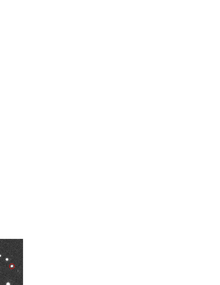
Figure 2: Herschel on its brightest phase, while observing NGC 5713. The image stamps cover an area of approximately $1^{\prime}\times 2^{\prime}$, while the time elapse between the images is $\approx 4$ minutes.

3.2 Registration

The images have then been registered (using the task fitrans) to the reference frame using the results yielded by the differential astrometry. Following the registration of the images, the flux levels of the images have also been scaled linearly to the same level. This was done by selecting several comparison stars and performing aperture photometry on these (involving the task fiphot). The mean of the aperture backgrounds have been subtracted from the respective images (yielding a zero mean background level) while the instrumental fluxes has been scaled appropriately to the flux level of the reference image (that was, in practice, the same as the one used as an astrometric reference). A master reference image was then built (employing the program ficombine), from every tenth of the individually registered and scaled images by taking the per-pixel median of these.

3.3 Astrometry and photometry of Herschel itself

Herschel itself was then searched by eye on $7\times 3$ frames (i.e. 3 subsequent images in 7 groups, spreading almost homogeneously through the whole observation). Using these coordinates as a hint for astrometry, the task fiphot was used to refine the pixel coordinates and then a third-order polynomial has been fitted to both the $X$ and $Y$ coordinates as the function of the time. We found that fitting a third order polynomial was sufficient at a certain level (i.e. the residuals were not larger than few tenths of a pixel) and this polynomial was used to interpolate the current position of the HSO between the frames were it was marginally or absolutely not detected. This interpolated coordinates have been exploited as a hint for a subsequent centroid determination (using the task fiphot). These refined centroid coordinates were then used as a photometric centroid, on which the actual aperture photometry was performed. In order to avoid the effect of nearby stars (that were crossed by Herschel apparently), this process has been done on differential images (i.e. the master reference image has been subtracted from each registered and scaled image before astrometry and photometry).

3.4 Almost-standard magnitudes

To have an accurate photometry, all of the nicely detected stars on the master reference image has been measured similarly (with the same aperture size as for Herschel) and using the cross-match lists from the absolute astrometry, we were able do determine the shift between the standard (USNO) and the instrumental magnitudes. Although this step sounds a bit optimistic (i.e. the flux levels derived from a CCD image without any filter has been adjusted to a photographic reference catalogue with a given filter and we neglect the effects of the color-dependent extinction), we found that the residual of this fit is not larger than $0.07^{\rm m}$. On can see the resulted light curve on Fig. 1. Image stamps showing Herschel itself on some of its brightest phases can be seen on Fig. 2, while the results of astrometry and photometry in the format of MPC are displayed on Table 1.

4 Discussion

In this draft some photometric and astrometric measurements for the Herschel Space Observatory have been presented. As it was discussed here, taking accurate photometry of HSO has some difficulties due to the fast apparent proper motion. Anyway, the presented photometric results confirm that the brightness variations of HSO (yielded by the telescope slews) is in accordance with the observation logs, and…and this is really reassuring.

References

- de Graauw et al. (2010) de Graauw, Th. et al. 2010, A&A, 518, 6
- Griffin et al. (2010) Griffin, M. J. et al. 2010, A&A, 518, 3
- Pál (2009) Pál, A. 2009, PhD thesis (arXiv:0906.3486)
- Pilbratt et al. (2010) Pilbratt, G. L. et al. 2010, A&A, 518, 1
- Poglitsch et al. (2010) Poglitsch, A. et al. 2010, A&A, 518, 2