Searching for comets on the World Wide Web:
The orbit of 17P/Holmes from the behavior of photographers

Abstract

We performed an image search for “Comet Holmes,” using the Yahoo! Web search engine, on 2010 April 1. Thousands of images were returned. We astrometrically calibrated—and therefore vetted—the images using the Astrometry.net system. The calibrated image pointings form a set of data points to which we can fit a test-particle orbit in the Solar System, marginalizing over image dates and detecting outliers. The approach is Bayesian and the model is, in essence, a model of how comet astrophotographers point their instruments. In this work, we do not measure the position of the comet within each image, but rather use the celestial position of the whole image to infer the orbit. We find very strong probabilistic constraints on the orbit, although slightly off the JPL ephemeris, probably due to limitations of our model. Hyperparameters of the model constrain the reliability of date meta-data and where in the image astrophotographers place the comet; we find that $\sim 70$ percent of the meta-data are correct and that the comet typically appears in the central third of the image footprint. This project demonstrates that discoveries and measurements can be made using data of extreme heterogeneity and unknown provenance. As the size and diversity of astronomical data sets continues to grow, approaches like ours will become more essential. This project also demonstrates that the Web is an enormous repository of astronomical information; and that if an object has been given a name and photographed thousands of times by observers who post their images on the Web, we can (re-)discover it and infer its dynamical properties.

1 Introduction

The Web bristles with billions of images: on Web pages, in public photo-sharing sites, on social networks, and in private email and file-sharing conversations. A tiny fraction but enormous number of these images are astronomical images—images of the night sky in which astronomical sources are visible. This is true even if we exclude from consideration scientific collections such as those of professional observatories and surveys and only count the images of hobbyists, amateurs, and sight-seers. In principle these images, taken together, contain an enormous amount of information about the astronomical sky. Of course they have no scientifically responsible provenance, have never been “calibrated” in any sense of that word, and were (mainly) taken for purposes that are not at all scientific. But having been generated from CCD-like measurements of the intensity field, they cannot help but contain important scientific information. The Web is, therefore, an enormous and virtually unexploited sky survey.

It is difficult to estimate the total number of astronomical images on the Web, and even harder to estimate the total data throughput (étendue or equivalent measure of scientific information content). However, by any estimate, it is extremely large. For example, image search results for common astronomical subjects include thousands of astronomical images. The flickr photo-sharing Web site has an astrometry group (administered by the Astrometry.net collaboration; more below) with more than $23,\!000$ photos, and its astronomy and astrophotography groups have more than $35,\!000$ and $45,\!000$ respectively. A search for the Orion Nebula on flickr returns more than 9000 images, which jointly contain significant information on very faint stars and nebular features. These numbers—derived solely from flickr searches—represent only a tiny fraction of the relevant Web content. Of course all these search results contain many non-astronomical images, diagrams, fake data, and duplicates, so use of them for science is non-trivial.

The technical obstacles to making use of Web data are immense: If anything has been learned from our interaction with electronic communication, it is that publisher-supplied or provider-supplied meta-data about Web content are consistently missing, misleading, in error, or obscure. Indeed, when it comes to the astronomical properties of imaging discovered on the Web, most providers do not even know what we want in terms of “meta-data”; we want calibration parameters relating to image date, astrometric coordinate system, photometric sensitivity, and point-spread function, and we want it in machine-readable form. The Virtual Astronomy Multimedia Project (VAMP, Gauthier et al. 2008) has defined a format for placing astrometric meta-data in image headers, but the goal of the project is to make “pretty pictures” searchable for education and public outreach purposes, rather than science. They do not consider the problem of producing or verifying calibration meta-data; they assume correct meta-data are provided along with the science images that are used to produce the pretty pictures. Even the Virtual Observatory (http://ivoa.net), which concentrates on astronomical meta-data, has no plan for ensuring that meta-data are correct, and has no machine-readable form for many quantities of great interest (such as the detailed point-spread-function model); we cannot expect the world’s amateur astrophotographers to be better organized.

Two important changes are occurring in astronomy that are opening up the possibility that we might exploit data collections as radically confusing as that of the entire Web. The first is that tools are beginning to appear that can perform completely hands-free data analysis tasks. The best example so far is the Astrometry.net system, which can take astronomical imaging of completely unknown provenance, and calibrate it astrometrically using the data in the image pixels alone (Lang et al. 2010).

The second change is that there has been an enormous increase in the amount and diversity of publicly available professional data—that is, calibrated, trustworthy, science-oriented data in observatory, sky-survey, and individual-investigator collections. These collections are so large and diverse that automated data analysis tools that can trivially interact with extremely heterogeneous data are necessary in many scientific domains. That is, much of the technology required for exploitation of the Web-as-sky-survey is required for any mature, data-intensive scientific investigation.

We have been exploring some of these ideas with the Astrometry.net project. Not only has the system calibrated thousands of images taken by amateurs and hobbyists, we have interfaced the system with flickr (Stumm et al., forthcoming). When a user adds an image to the “astrometry” group, an automated “bot” downloads the image, calibrates it with Astrometry.net, and then posts machine-readable calibration results to the image’s page on flickr; these have been dubbed “astro-tags”. The bot also adds annotations to the image, marking named stars and galaxies from the Messier and NGC/IC catalogs. We make use of the flickr Application Programming Interface (API); many image and data-sharing sites offer APIs that allow scriptable access to the data they hold. The success of our flickr bot suggests that automated maintenance of a heterogeneous crowd-sourced sky survey might be possible in the future.

In this paper, we explore some of the ideas around the Web-as-sky-survey, by performing a scientific investigation of Comet 17P/Holmes using Web-discovered, human-viewable (JPEG) images alone. Although we do in principle learn things about Comet Holmes, our main interest is in developing and testing new technologies for observational astrophysics. This project leverages the tendency of humans to point their cameras and telescopes towards interesting things, the ability of Yahoo! (or any other search engine) to classify and organize their images, and the ability of Astrometry.net to figure out after the fact where they were pointing. What we do is related to other citizen-science projects, like the GalaxyZoo (Lintott et al. 2011) or the monitoring projects of the AAVSO (http://aavso.org), except that the participants here are entirely unwitting. We end up showing that there is substantial scientific content in the data taken by citizen observers, even if they have not committed to particular scientific goals; we also show that it is possible to extract scientific information from observations of which the provenance is unknown.

2 Data and calibration

Our data collection began with a search of the World Wide Web. We used the pYsearch (Hedstrom 2007) code to access the Yahoo! Web Search service. On 2010 April 1, we searched for JPEG-format images using the query phrase “Comet Holmes.” Due to a dramatic brightening during its 2007 apparition, Comet Holmes became a very popular and accessible target for astrophotographers, so many images are available on the Web. Our search yielded approximately $10,\!000$ total results, but the Yahoo! Web Search API allowed only $1000$ results to be retrieved per query. In order to broaden the result set, we performed an additional set of searches: For each Web site containing an image in the original set of results, we performed a query that was limited to that Web site. These queries, performed later on 2010 April 16, produced an additional $2741$ results (including some duplicates), for a total of $2476$ unique results. See Figure 1 for some example images.

Next, we retrieved the images on 2010 April 16. This yielded a total of $2309$ valid JPEG images. After removing byte-identical images, $2241$ unique images remained. We then ran the Astrometry.net code on each image to perform astrometric calibration. $1299$ images were recognized as images of the night sky and astrometrically calibrated. These images form the data set we use in our analysis below. Figure 2 shows the footprints of the images on the sky.

Many of the images in this data set are annotated images or diagrams such as finding charts or illustrations of the comet’s orbit. Some of these diagrams were recognized by Astrometry.net as images of the sky. This can be seen in the co-added image in Figure 2, where there are clearly lines connecting the stars that form the constellation Perseus.

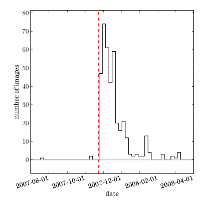
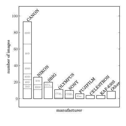
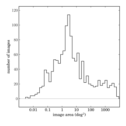
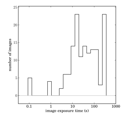
Figure 3: Top-left: The timestamps in the EXIF headers of the images in our data set. $422$ of the $1299$ images have timestamps; $394$ are within the range plotted here. The dashed line marks 2007 Oct 24, the date of the comet’s outburst and dramatic brightening (Buzzi et al. 2007). Top-right: The distribution of camera manufacturers listed in the EXIF headers (for the 183 images containing manufacturer information). Bottom-left: The distribution of image angular sizes in our data set, according to Astrometry.net. Bottom-right: The distribution of exposure times in our data set, according to EXIF headers (for the 149 images containing an exposure time entry).

Of the $1299$ images in our data set, $422$ have timestamps in the image headers (“Exchangeable image file format” or EXIF headers). The distribution of timestamps is shown in Figure 3. On 2007 Oct 24, Comet 17P/Holmes brightened by more than 10 mag (Buzzi et al. 2007), generating considerable public interest and making it a very popular and accessible observing target in the amateur astronomy community. The distribution of image timestamps shows a large spike at this time.

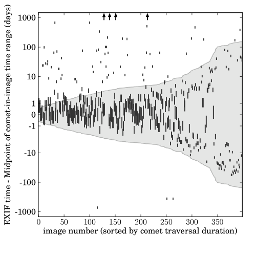
Figure 4: Evaluation of the accuracy of the timestamps in the image EXIF headers. For each image, we computed the range of times that the comet appeared inside the celestial-coordinate bounds of the image; that is the shaded gray region, which is vertically centered at zero. The images are sorted so that this envelope is monotonic. The EXIF timestamp for each image is shown as a bar of height one day (since EXIF has no time zone specification, this is our intrinsic uncertainty), plus a minimum size to make all the markers visible. If the EXIF timestamps were correct and set to UT, the position of the bar within the gray region would indicate the position of the comet within the image. Most of the bars touch the gray region, indicating that the majority of the EXIF timestamps are consistent (that is, the comet would indeed appear within the image at the stamped time), and the inconsistent times are almost all later; perhaps these timestamps mark times at which the image was edited. The apparent bifurcation toward the right side of the plot is due to the nonlinear (arcsinh) mapping we have applied to the vertical axis. Of the $422$ images with timestamps, $23$ did not intersect the comet’s trajectory (during the 2007 apparition); this plot shows the $399$ that did intersect the trajectory. The arrows at the top of the plot show the locations of $4$ images outside the plot bounds.

We evaluate the accuracy of the image timestamps by asking, for each image, whether the comet would appear within the celestial-coordinate bounds of the image at its stamped time. We find that the majority of the timestamps are consistent, and that inconsistent timestamps are typically late rather than early; we assume this is because some of the images have been post-processed and the timestamp represents the time the image was last edited rather than the time the image was taken. See Figure 4.

Figure 3 shows the distribution of angular scales of the images in our data set. The distribution peaks around $3$ square degrees. Also shown is the distribution of exposure times reported in the EXIF headers.

3 Orbit inference

We take the approach of generative modeling; that is, we construct a well-defined approximation to the probability of the data given the model. We take the “data” to be the pointing (on the sky) of each astrometrically calibrated image (as determined by Astrometry.net); recall that the goal is to use the behavior of astrophotographers (in pointing their cameras) to find the gravitational orbits of objects in the sky. We treat the time at which each image is taken as a hidden “nuisance” parameter.

For each image $i$ there is a pointing $\boldsymbol{\alpha}_{i}$ (two-dimensional position or celestial coordinates on the sky). These are the data. The image was taken at time $t_{i}$, and has image parameters $\boldsymbol{\Omega}_{i}$ (camera plate scale, image size, orientation, and reported EXIF timestamp if there is one), taken to be known. In addition, the comet has orbital parameters $\boldsymbol{\omega}$, which can be thought of as semi-major axis, eccentricity, inclination, longitudes, etc., or equivalently a 3-dimensional position $\boldsymbol{x}$ and velocity $\boldsymbol{v}$ at a chosen epoch. We choose the latter for inference simplicity, and use as the epoch JD $2454416.0$ (2007 Nov 12). Finally, there are three additional nuisance hyperparameters $\boldsymbol{\theta}$ that will appear as we go. In this work we consider only the 2007 apparition of the comet. Our data set does include at least one image of the comet during an earlier apparition (1892; see Figure 1(1)), but we chose not to attempt to fit multiple apparitions.

The single-image likelihood $p(\boldsymbol{\alpha}_{i}|\boldsymbol{\Omega}_{i},\boldsymbol{\omega},\boldsymbol{\theta})$ is a marginalization over time $t_{i}$ of the time-dependent single-image likelihood, $p(\boldsymbol{\alpha}_{i}|t_{i},\boldsymbol{\Omega}_{i},\boldsymbol{\omega},\boldsymbol{\theta})$:

$$\displaystyle p(\boldsymbol{\alpha}_{i}|\boldsymbol{\Omega}_{i},\boldsymbol{\omega},\boldsymbol{\theta}) = \int p(\boldsymbol{\alpha}_{i}|t_{i},\boldsymbol{\Omega}_{i},\boldsymbol{\omega},\boldsymbol{\theta})\,p(t_{i}|\boldsymbol{\Omega}_{i},\boldsymbol{\theta})\,dt_{i}\quad,$$ (1)

where the time-dependent single-image likelihood is a mixture of “foreground” (inlier) and “background” (outlier) components:

$$\displaystyle p(\boldsymbol{\alpha}_{i}|t_{i},\boldsymbol{\Omega}_{i},\boldsymbol{\omega},\boldsymbol{\theta}) = p_{\mathrm{good}}\,p_{\mathrm{fg}}(\boldsymbol{\alpha}_{i}|t_{i},\boldsymbol{\Omega}_{i},\boldsymbol{\omega},\boldsymbol{\theta})+[1-p_{\mathrm{good}}]\,p_{\mathrm{bg}}(\boldsymbol{\alpha}_{i})\quad.$$ (2)

The components are:

$$\displaystyle p_{\mathrm{fg}}(\boldsymbol{\alpha}_{i}|t_{i},\boldsymbol{\Omega}_{i},\boldsymbol{\omega},\boldsymbol{\theta}) = \left\{\begin{array}[]{ll}[\eta\,\Omega_{i}]^{-1}&\mbox{comet in $\eta$ sub-image}\\ 0&\mbox{comet not in $\eta$ sub-image}\end{array}\right.$$ (5)

$$p_{\mathrm{bg}}(\boldsymbol{\alpha}_{i}) = [4\pi]^{-1}\quad.$$ (6)

The hyperparameters $\boldsymbol{\theta}$ include $p_{\mathrm{good}}$, $\eta$, and $p_{\mathrm{EXIF}}$ (discussed below). Here, $p_{\mathrm{good}}$ is the probability that the image really is a picture intentionally taken of (generated by) the comet, $p_{\mathrm{fg}}(\cdot)$ is a “foreground” model, which gives high likelihood when the comet (with orbital parameters $\boldsymbol{\omega}$ at time $t_{i}$) is inside the image, and $p_{\mathrm{bg}}(\cdot)$ is a “background” model, with no dependence on the comet or time, that describes images that are in our data set but do not contain the comet (perhaps because they were incorrectly returned by the Web search engine). The $4\pi$ in $p_{\mathrm{bg}}(\cdot)$ is the solid angle of the whole sky. The hyperparameter $\eta$ (subject to $0<\eta<1$) controls the fractional size of the central region of an image in which astrophotographers place comet subjects, $\Omega_{i}$ is the solid angle covered by image $i$, and the “$\eta$ sub-image” is the central $\eta$ of the image. In detail, we define the $\eta$ sub-image to have the same aspect ratio as the whole image, centered at the same point, but smaller in angular size by $\sqrt{\eta}$ along both dimensions.

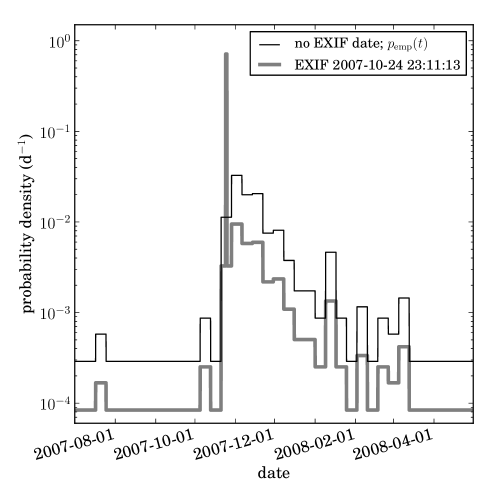
Figure 5: The time prior PDF $p_{\mathrm{emp}}(t)$ used for images with no EXIF date information (dark line) and the time prior PDF for an image with a particular EXIF date (lighter line). The latter is a mixture of $p_{\mathrm{emp}}(t)$ and a top-hat of width one day centered on the EXIF date and fractional weight $p_{\mathrm{EXIF}}=0.71$. We use a width of one day because the EXIF standard does not permit the time zone to be specified. The function $p_{\mathrm{emp}}(t)$ is based on the distribution of reported EXIF dates shown in Figure 3; details in the text.

Our Bayesian prior probability distribution function (PDF) over time, $p(t_{i}|\boldsymbol{\Omega}_{i},\boldsymbol{\theta})$, turns out to be crucial to good inference in this problem, in part because trivial or wrongly uninformative time PDFs lead to highly biased answers, a point to which we will return below. We expect that a large fraction of the image EXIF timestamps (where they exist) are correct, but at the same time we cannot trust them completely. We construct an empirical “cheater” prior $p_{\mathrm{emp}}(t)$ based on the empirical histogram of extant EXIF timestamps as follows: We construct a grid of non-overlapping bins in time of width 8 d between $t_{\mathrm{min}}=$2007 July 1 and $t_{\mathrm{max}}=$2008 May 1. We count EXIF timestamps in these bins, and then add 1 to every bin (so no bins have counts of zero). We then normalize so that the integral of $p_{\mathrm{emp}}(t)$ is unity. This empirical prior is shown in Figure 5. Given any image $i$ with image parameters $\boldsymbol{\Omega}_{i}$, the PDF for time $t_{i}$ is

$$\displaystyle p(t_{i}|\boldsymbol{\Omega}_{i},\boldsymbol{\theta}) = \left\{\begin{array}[]{ll}p_{\mathrm{emp}}(t_{i})&\mbox{if no $t_{\mathrm{EXIF}}$ in $\boldsymbol{\Omega}_{i}$}\\ p_{\mathrm{EXIF}}\,p(t_{i}|t_{\mathrm{EXIF}})+[1-p_{\mathrm{EXIF}}]\,p_{\mathrm{emp}}(t_{i})&\mbox{if $t_{\mathrm{EXIF}}$ in $\boldsymbol{\Omega}_{i}$}\\ \end{array}\right.$$ (9)

$$p(t_{i}|t_{\mathrm{EXIF}}) = \mathrm{uniform}(t_{i}|t_{\mathrm{EXIF}}-[0.5~{}\mathrm{d}],\,t_{\mathrm{EXIF}}+[0.5~{}\mathrm{d}])\quad,$$ (10)

where $p_{\mathrm{EXIF}}$ is the third hyperparameter in $\boldsymbol{\theta}$ and the probability that a given EXIF timestamp is reliable, $\mathrm{uniform}(x|A,B)$ is the top-hat or uniform PDF for $x$ between $A$ and $B$, $t_{\mathrm{EXIF}}$ is the reported EXIF timestamp, and we have subtracted and added $0.5~{}\mathrm{d}$ because the EXIF format contains no time zone information and this is the span of possible time zones. In short, if an image does not contain an EXIF timestamp, the model uses the empirical distribution of time stamps. If an image does contain an EXIF timestamp, it is likely to be correct so the model assigns fraction $p_{\mathrm{EXIF}}$ of the probability mass to a 24-hour window around the timestamp, but also hedges by including fraction $1-p_{\mathrm{EXIF}}$ of the empirical distribution. An example is shown in Figure 5.

The single-image likelihood $p(\boldsymbol{\alpha}_{i}|\boldsymbol{\Omega}_{i},\boldsymbol{\omega},\boldsymbol{\theta})$ is the probability that an image would be taken at coordinates $\boldsymbol{\alpha}_{i}$ given the camera properties $\boldsymbol{\Omega}_{i}$, the comet’s trajectory $\boldsymbol{\omega}$, and our model hyperparameters $\boldsymbol{\theta}$, integrated (marginalized) over the time period we consider. We do not specify the exact time $t_{i}$ of each image; we instead specify a probability distribution of times and integrate over it (and this integration requires us to be Bayesian). In order to evaluate this likelihood, we compute the comet trajectory on a fine time grid and perform the time integral numerically as a sum over grid points. For dynamical integration we use a Keplerian two-body celestial mechanics code implemented in Python by Astrometry.net for both the comet and the Earth–Moon barycenter (EMB); we take the initial conditions of the EMB from JD $2454101.5$ (2007 Jan 1). For simplicity we take the EMB to be the observer’s location, thus ignoring the effect of parallax. At the precision of the data, the finite light-travel time in the Solar System is significant; we include it when we consider the observed position of the comet as a function of time. For the numerical integrals, we simply convert observed Solar-system directions to positions on the celestial sphere, and positions on the celestial sphere to image positions (to determine whether particular comet instances are inside particular images) with the Astrometry.net world-coordinate system libraries (Lang et al. 2010). Outliers—images that do not contain the comet—will only by chance intersect the comet trajectory so will have low likelihood under the foreground model $p_{\mathrm{fg}}(\cdot)$; the background model $p_{\mathrm{bg}}(\cdot)$, which has no dependence on the orbital parameters, will dominate the likelihood. As with the time $t_{i}$, we need not explicitly estimate whether any given image is an outlier; we instead model the data as a mixture of the foreground distribution (“inliers”) and a background distribution (“outliers”), and sum (marginalize) over the two possibilities.

The total likelihood is the product of the individual-image marginalized likelihoods, and the posterior PDF for the parameters $\boldsymbol{\omega}$ and $\boldsymbol{\theta}$ is proportional to the total likelihood times a prior. We take this prior to be Gaussian in comet position $\boldsymbol{x}$ with three-dimensional isotropic Gaussian variance of $[1~{}\mathrm{AU}]^{2}$, a beta distribution in squared velocity $v^{2}\equiv\boldsymbol{v}\cdot\boldsymbol{v}$ between $v^{2}=0$ and the $v^{2}$ that just unbinds the comet, with beta-distribution parameters $\alpha=1$ and $\beta=3$. We take the prior to be flat in the range 0 to 1 for the probability hyperparameters $p_{\mathrm{good}}$ and $p_{\mathrm{EXIF}}$ and (improperly) flat in $\ln(\eta)$ for the fractional hyperparameter $\eta$. These 9 parameters (three position components, three velocity components, two probabilities, and one fraction) are the parameters in which we perform our Markov Chain Monte Carlo (MCMC) sampling. We perform the sampling with a Python implementation (Foreman–Mackey et al. 2012) of an affine-invariant ensemble sampler (Goodman et al. 2010, Hou et al. 2012) using an ensemble of 64 walkers and Python multiprocessor support.

We initialize the MCMC using the following heuristic. Since we know we have many images taken during a short window around the comet’s outburst, we select images with timestamps within a week of the median date. Of these images, we keep those whose centers are within 5 degrees of the median right ascension and declination. This gives us a set of $136$ images to which we fit lines for right ascension and declination with respect to time, weighting by the inverse image extents. Assuming the comet is $1~{}\mathrm{AU}$ away from Earth and moving perpendicular to the line of sight, we convert the projected position to a three-dimensional position $\boldsymbol{x}_{0}$ and velocity $\boldsymbol{v}_{0}$ at the epoch. We choose eyeballed-sensible initial values for the hyperparameters: ${p_{\mathrm{good}}}_{0}=0.85$, ${p_{\mathrm{EXIF}}}_{0}=0.75$, and ${\eta}_{0}=0.4$. To initialize the ensemble of MCMC samples, we add Gaussian noise with standard deviation $10^{-5}~{}\mathrm{AU}$ to the position $\boldsymbol{x}_{0}$, $10^{-3}~{}\mathrm{AU}/\mathrm{yr}$ to the velocity $\boldsymbol{v}_{0}$, and $10^{-2}$ to each of ${p_{\mathrm{good}}}_{0}$, ${p_{\mathrm{EXIF}}}_{0}$, and ${\eta}_{0}$. The details of the initialization are not critical; the MCMC sampler will explore the parameter space and find a good solution in a reasonable number of iterations as long as we initialize it somewhat near the solution.

There are several substantial limitations to this model: The prior does not even come close to representing our true prior knowledge about comets, particularly ones that are observed by photographers and posted to the Web. The total likelihood (being a product of individual-image likelihoods) assumes all the data are independent, but in reality some of the images found by the Web search are repeats, duplicates, or derived images from others. Most importantly, we make no attempt to find the comet in the image. This is a model of how astronomers point their cameras, not of the visible comet itself.

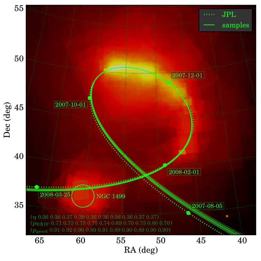
Figure 6: Image footprints with JPL ephemeris and inferred orbits superimposed. The solid lines show 16 samples from the posterior PDF for the parameters. The values for the hyperparameters $p_{\mathrm{good}}$, $p_{\mathrm{EXIF}}$, and $\eta$ (see text for definitions) for some of the samples are listed at the bottom of the plot. The background shows the pixel density as in Figure 2.

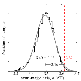
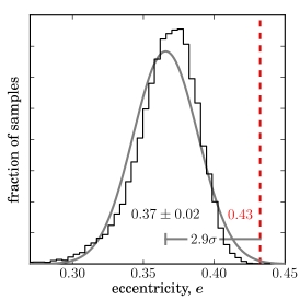
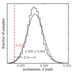
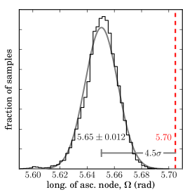
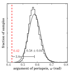
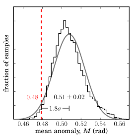
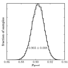
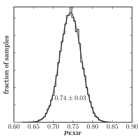
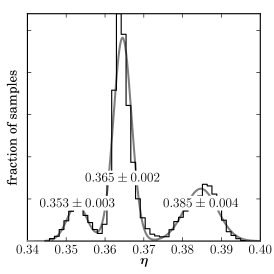
Figure 7: Top two rows: Orbital parameters inferred by our method (histogram and best-fit Gaussian), and JPL ephemeris values (vertical bar). Most of our inferred parameter distributions are a few standard deviations from the JPL values. In the next figure we show that our inferred trajectory is closer to the JPL trajectory than the differences in orbital elements might suggest. Bottom row: Our inferred hyper-parameters: $p_{\mathrm{good}}$, the probability that an image is an image of the comet (that is, was generated by the foreground probability distribution $p_{\mathrm{fg}}$); $p_{\mathrm{EXIF}}$, the probability that a timestamp in an image EXIF header is correct; and $\eta$, the central fraction of the image area in which the comet appears.

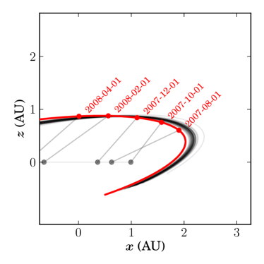
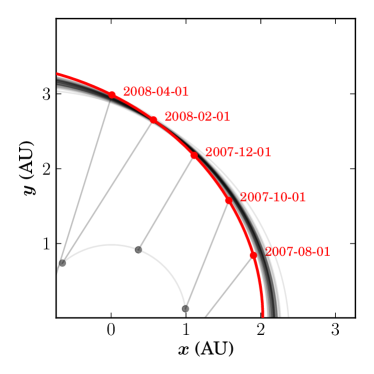
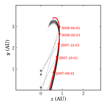
Figure 8: Three-dimensional inferred orbit (thin lines) and JPL orbit (dashed line) in heliocentric equatorial coordinates. We have plotted 32 samples from our inferred orbit distribution to show the scatter. Also shown is the JPL orbit of the Earth-Moon barycenter. Our inferred orbit captures the general shape of the trajectory of the comet, and is relatively unconstrained at early and late times (when we have no data).

The results of the inference are shown in Figure 6 as a set of sample trajectories drawn from the Markov chain. These samples are effectively drawn from the posterior PDF marginalized over the hyperparameters. The small dispersion among the samples show that the data—just the pointings of a set of heterogeneous images—are incredibly informative about the comet orbit. In Figure 7 we show our estimates for the standard orbital elements, along with the values from the Horizons system from the Jet Propulsion Lab (JPL; Giorgini et al. 1996), which we take to be authoritative. Most of our parameter estimates are a few standard deviations away from the JPL values. Figure 8 shows that the three-dimensional orbit we infer is quite close to the JPL orbit in the regions where we have data, and the variance in our inferred orbit correctly increases in the regions where we lack data.

4 Discussion

We have shown that if a Solar System body has been named and hundreds of astrophotographers around the world have deliberately photographed it, we can recover its dynamical properties by a Web search operation followed by a large amount of computation. All the inference is done on image positions; we never look at the content of the images at all. This effectively makes the model a model of astrophotographers, because the image pointings are a record of where human observers pointed their telescopes and cameras. The six dynamical parameters are parameters of the comet to be sure, but the three hyperparameters are affected by human behavior as well as by properties of the comet. The probability $p_{\mathrm{good}}$ relates to the purity of image search on the Web, the probability $p_{\mathrm{EXIF}}$ relates to the reliability of astrophotographers’ Web-published image meta-data, and the fraction $\eta$ relates to how astrophotographers frame their images. We find hyperparameter $p_{\mathrm{good}}\sim 0.9$, which indicates that a large majority of the images returned by the Web search and recognized by Astrometry.net do indeed contain Comet Holmes. We find $p_{\mathrm{EXIF}}\sim 0.7$, indicating that when images have timestamps in their headers, they are often correct. We find $\eta\sim 0.36$, indicating that astrophotographers tend to place Comet Holmes in the middle third of the image area.

We expect that these hyperparameters will vary for different Web search engines, query phrases, and comets. Comets with distinctive names are likely to be better indexed by search engines, faint comets are likely to be photographed by different populations of observers, and comets with long tails are likely to be framed differently in photographs. We expect that searching for the phrase “17P/Holmes” rather than “Comet Holmes,” for example, might result in images from more technical astronomy Web sites rather than the popular press. As a result, we might find that a higher fraction of the images contain the comet, leading to a higher inferred $p_{\mathrm{good}}$; we might find that the images have different distributions of angular extents and different framing, resulting in different $\eta$; and we might expect that more of the images were captured with telescope-mounted CCDs, saved in non-JPEG formats and subsequently processed to produce the pretty picture, perhaps resulting in different timestamp properties and therefore $p_{\mathrm{EXIF}}$.

If we omit $\eta$ from our model (i.e., assume it is unity), we effectively ignore the fact that astrophotographers frame their subjects, and this in turn increases the positional uncertainty of the comet, which results in poorer constraints on the orbit of the comet. By including $\eta$, we give our model the freedom to learn how astrophotographers compose their images. The model prefers to set $\eta$ to a rather small fraction, indicating that this freedom is useful. Including $\eta$ means that if the comet appears in the corner of an image, the image will be treated as an outlier and will not contribute to constraining the orbit. However, this loss of constraining power is balanced by stronger constraints from all images in which the comet appears near the center. In Figure 7, there are three peaks in the histogram of $\eta$ values. We assume the two sub-dominant peaks correspond to $\eta$ values that omit one image or include one additional image in the solution, relative to the dominant peak.

The model is exceedingly crude, and the fact that our results are biased (the samples in Figure 6 are offset from the JPL trajectory) is probably in part related to this crudeness. The centering model is extremely crude; in reality there is a distribution of astrophotographers’ behavior that it ought to describe. The time model involves a hard-set empirical prior that is not justified and ought to be simultaneously optimized and marginalized out in the inference (this would be a form of hierarchical inference like in Hogg et al. 2010). The time-zone model (flat across all time zones) is also not realistic, since some time zones are much more populated with photographers than others. Along those same lines, there is an enormous amount of external information (weather data and visibility calculations) that could further constrain the possible times and time zones. As with time zones, we do not attempt to model the positions of the astrophotographers relative to the Earth-Moon barycenter. By ignoring the resulting parallax, we incur errors of about $5$ arcsecond in our estimate of the comet’s position.

Another crudeness is in the assumption of independent and identically distributed draws in the likelihood. This is not true in that some of the Web images we find are crops, edits, or diagrams made from other Web images. That is, each image is not guaranteed to be an independent datum.

Our model that astrophotographers tend to place their subjects in the center of their images ignores the fact that conjunctions of astronomical objects on the sky are often targets of interest. We suspect that we see this effect in our data set. When Comet Holmes passed near the California Nebula (NGC 1499), many photographers captured the conjunction. In Figure 6 this overdensity of images can be seen near the marked location of NGC 1499. The nebula appeared below the comet (at lower Dec), and it appears that our inferred comet trajectories have been pulled down as a result.

In some sense, this project is a citizen-science project, because it does science with data generated by non-scientists. However, it is very different from projects like SETI@Home (Korpela et al. 2009) because it makes use of participants’ intelligence, not just hardware. It is very different from projects like GalaxyZoo (Lintott et al. 2011) because it makes use of specialized astronomy knowledge among the participants; one must be a relatively avid astronomer to usefully contribute. It is very different from the projects of the AAVSO (http://aavso.org) or MicroFUN (Gould 2008) because the observers observed for reasons (for all we know) completely unrelated to our scientific goals. It is different from all of these projects in that the participants contributed unwittingly.

One interesting and ill-understood aspect of a citizen-science project of this type—where the participants are not aware that they are involved—relates to giving proper credit and obtaining proper permissions to use the images. We obtained permission to show the images shown in Figure 1 but we did not even attempt to get any permissions for the majority of the $2241$ images we touched in the analysis. One encouraging lesson from this project is that the photographers we did contact were very supportive: Not one rejected our request for permissions; typical responses expressed enthusiasm about being involved in a scientific paper; the majority asked to see the manuscript when it appears; some sent updated images or suggestions about which images to use; and a few offered details about the data analysis and processing that was performed. A less encouraging lesson is that Web image search APIs have an uncertain future: The Yahoo! Web Search API is being decommissioned, as is the Google Image Search API.

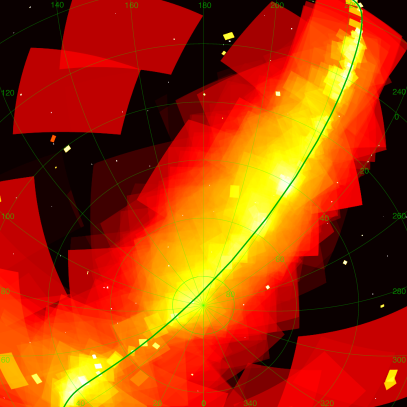
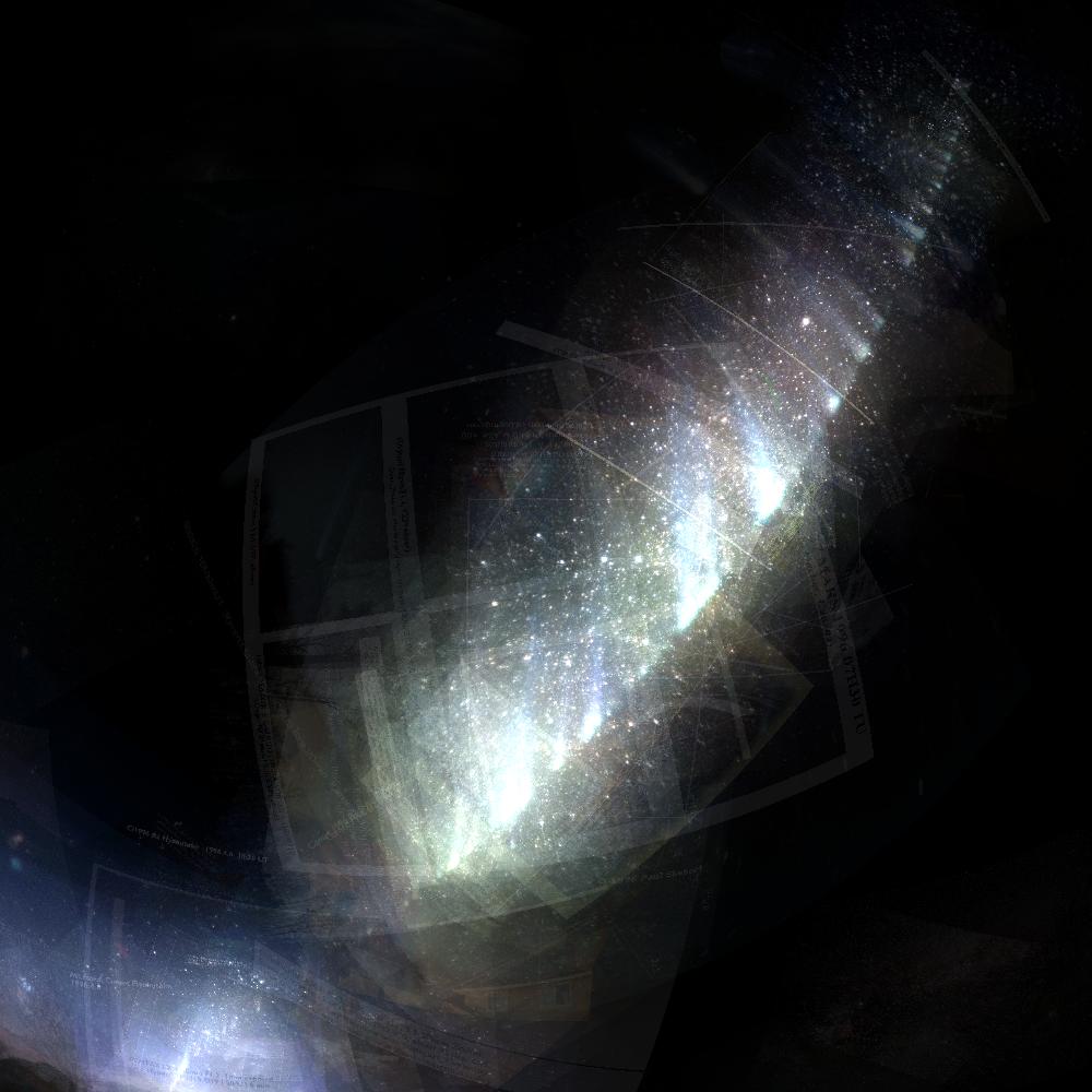
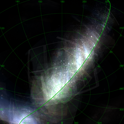
Figure 9: Same as Figure 2 but now for images found by a similar Web search for “Comet Hyakutake”. The search, performed on 2010 Oct 2, produced $1481$ JPEG images, of which $1019$ were recognized by Astrometry.net as images of the night sky. Top: Pixel density map, with a log stretch. The most heavily imaged areas appear in $152$ images. The projection is zenithal equidistant (FITS WCS code “ARC”, Calabretta & Greisen 2002). Bottom: Co-added images. The spectacular tail of the comet is clearly visible, as are many text labels, annotations, and image borders. The right panels show the same images as the left panels but with a coordinate grid and the trajectory of the JPL ephemeris.

The biggest lesson is that there is enormous information about astronomy available in uncurated non-professional images on the Web. We have only scratched this surface. Think how much better we could have done if we had gone into the images and actually made some attempt at detecting the comet! Figure 2 shows that there is far more information inside the images than in just the footprints. Figure 9 shows that there is a similarly informative body of images of Comet C/1996 B2 (Hyakutake). We have also noticed that there are thousands of images of the Orion Nebula on flickr alone, and thousands more elsewhere on the Web; the joint information in this body of images (about the nebula and about time-domain activity therein) must be staggering. Perhaps this is not surprising given the large amount of telescope aperture and detector area owned by avid photographers. We have learned that we can do high-quality quantitative astrophysics with images of unknown provenance on the Web. Is it possible to build from these images a true sky survey? We expect the answer is “yes”.

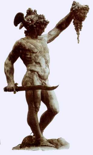
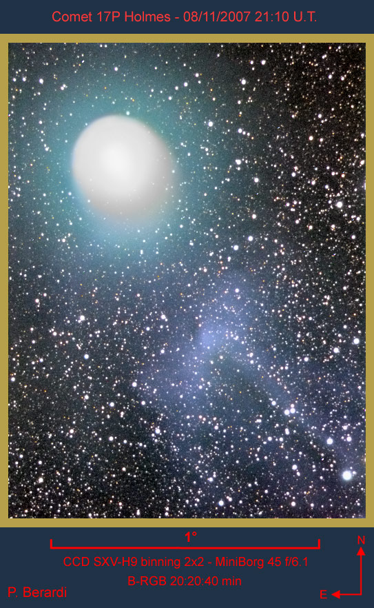
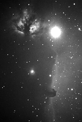
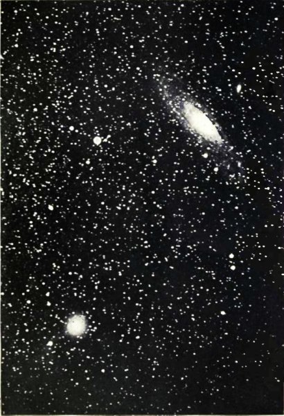
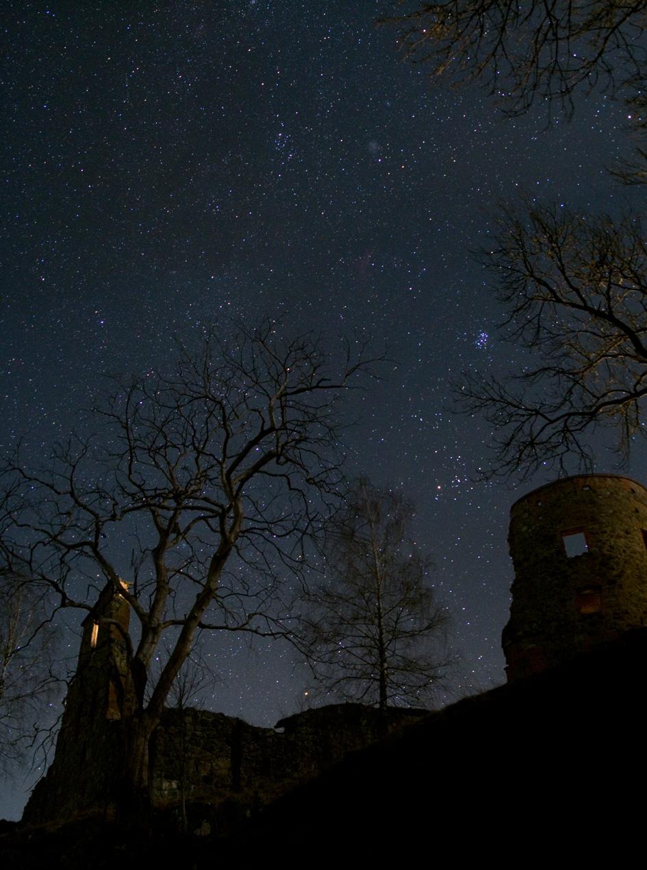
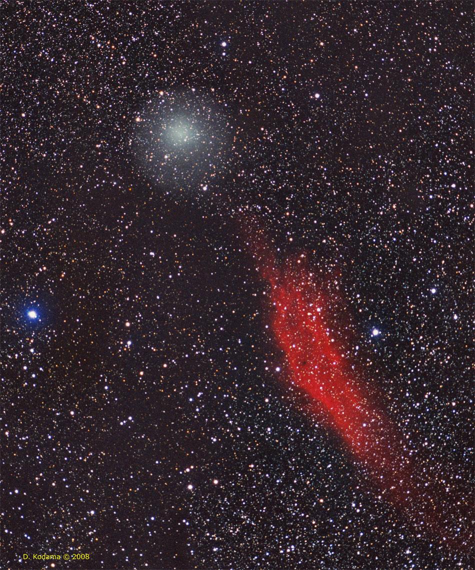
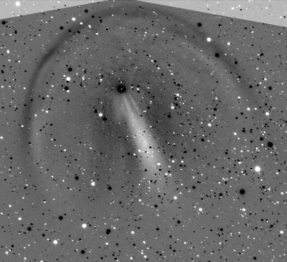
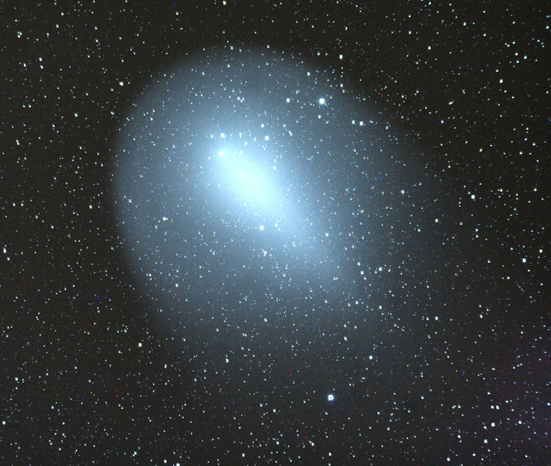
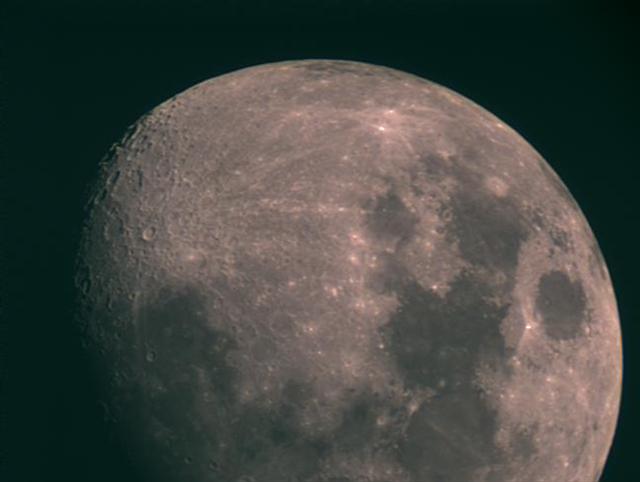
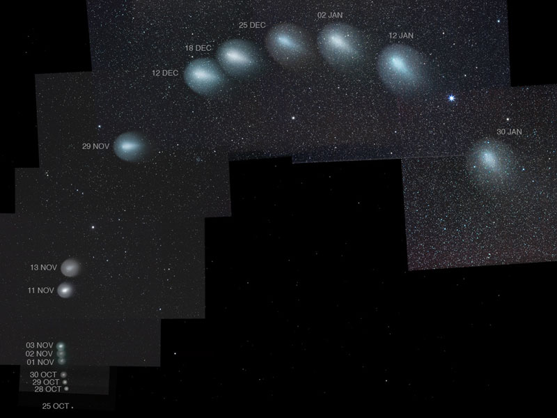
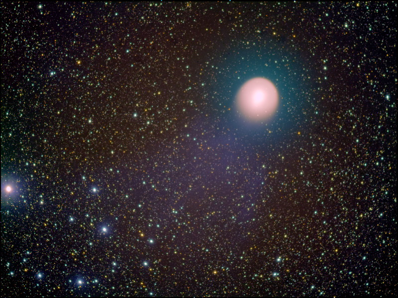
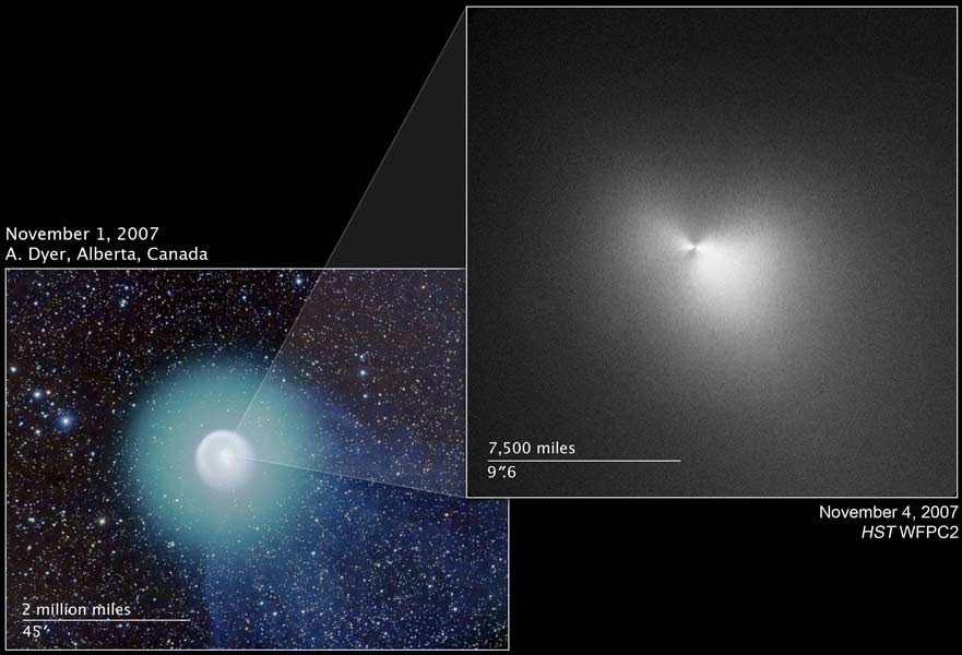
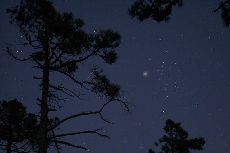
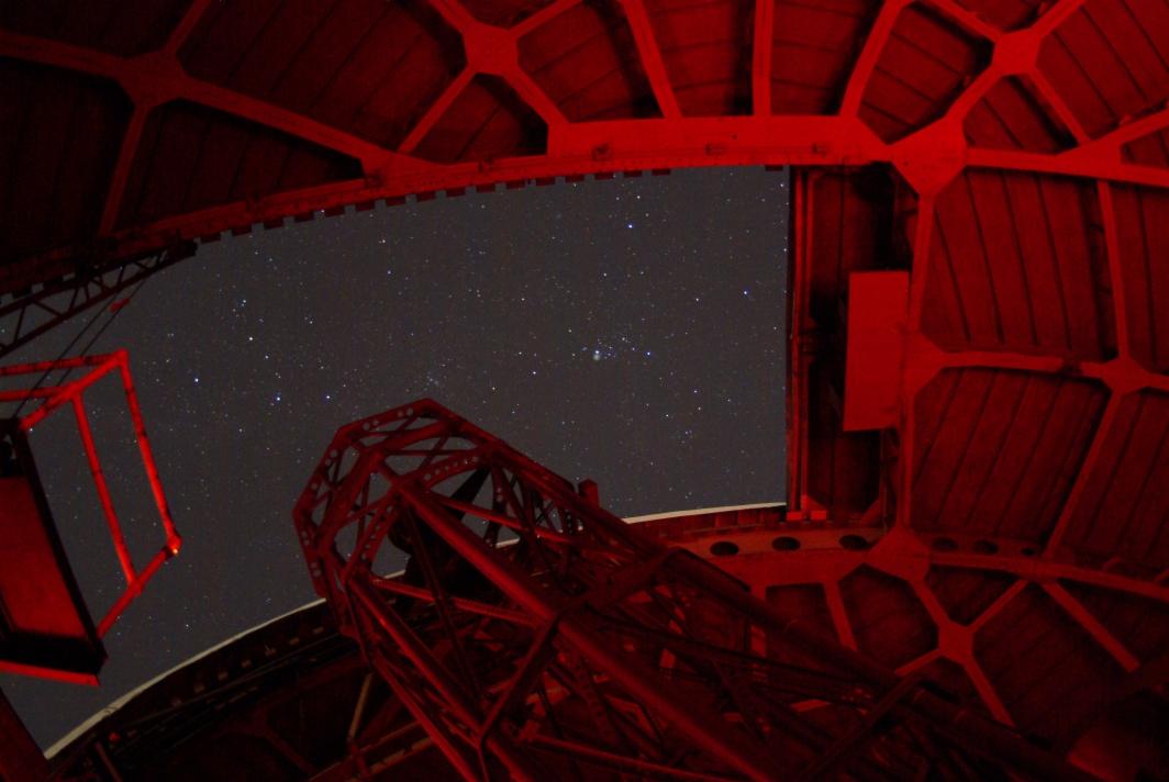
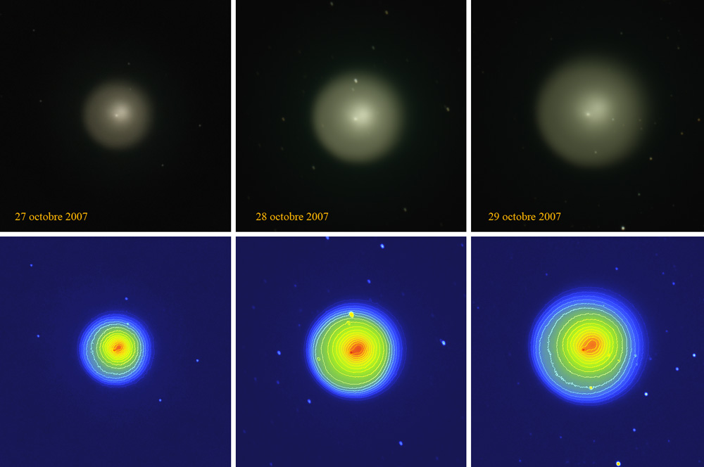
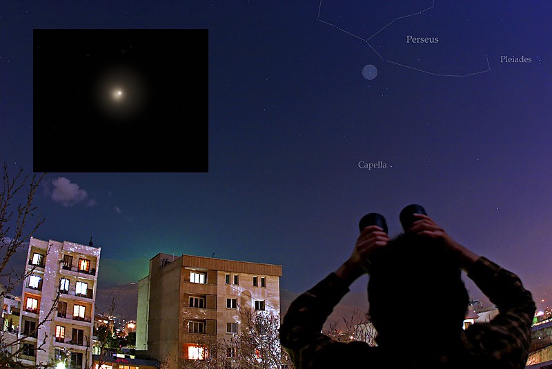
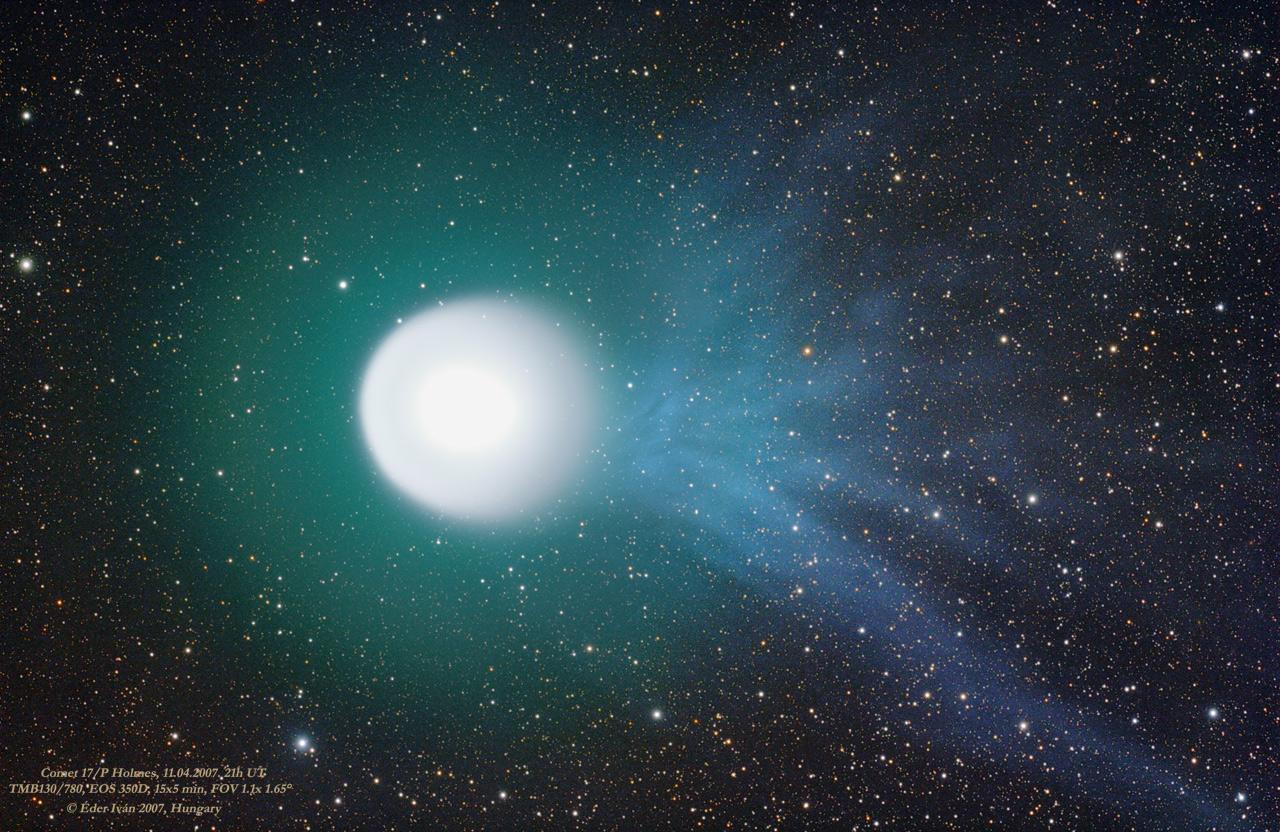
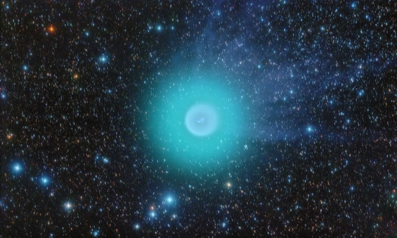
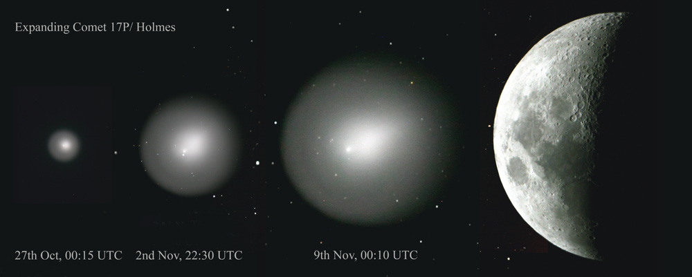
$\ast$(a)  (b)  $\ast$(c)  (d)  (e)  (f)  (g)  (h)  $\ast$(i)  $\ast$(j)  $\ast$(k)  $\ast$(l)  (m)  (n)  $\ast$(o)  (p)  (q)  $\ast$(r)  $\ast$(s)  (t)  (u)  $\ast$(v)  $\ast$(w) 

Figure 1: Example images…[caption next page]

Figure 1: [figure previous page] Example images from the image search. Here we have highlighted the diversity of the images; the majority are in fact high-quality, narrow-field images of the comet, such as (1), (1), (1), and (1). Images that did not calibrate successfully with Astrometry.net (and therefore were not used as data in this study) are marked with asterisks. Notice that images (1), (1), and (1) all were successfully calibrated and were used in the analysis. Image (1) shows a statue of Perseus, a constellation through which Comet Holmes traveled during its 2007 approach. Image (1) is from the year 1892, shortly after the discovery of Comet Holmes. Although it was calibrated and used in our analysis, this image was identified as an outlier since we are fitting only the 2007 apparition of the comet. Image (1) includes the California nebula (NGC 1499). Credits: (1) copyright 2000–2005 Gods, Heroes, and Myth (http://www.gods-heros-myth.com); (1) Paolo Berardi; (1) Amateur Astronomers, Inc. Research Committee (http://asterism.org); (1) Edward Emerson Barnard (Ball 1905); (1) copyright P.-M. Hedén (http://www.clearskies.se); (1) copyright Dave Kodama (http://astrocamera.net); (1) TOC Observatory (http://tocobs.org); (1) copyright Fay Saunders; (1) Bruce Card, Aldrich Astronomical Society, Worcester MA; (1) NASA, JPL-Caltech, W. Reach (SSC-Caltech); (1) copyright Julián Cantarelli; (1) copyright 2007, 2008 John F. Pane (http://holmes.johnpane.com); (1) copyright Tyler Allred (http://allred-astro.com); (1) Joe Orman; (1) NASA, ESA, and H. Weaver (The Johns Hopkins University Applied Physics Laboratory), and A. Dyer, Alberta, Canada; (1) copyright Vincent Jacques (http://vjac.free.fr/skyshows); (1) Jimmy Westlake, Colorado Mountain College; (1) Stephane Zoll (http://astrosurf.com/zoll); (1) Babak Tafreshi / TWAN (http://twanight.org); (1) Ivan Eder (http://eder.csillagaszat.hu); (1) Vicent Peris (OAUV), José Luis Lamadrid (CEFCA); (1) copyright Thorsten Boeckel (http://tboeckel.de); (1) D. J. Barry, Department of Astronomy, Cornell University.

 

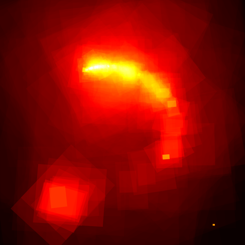
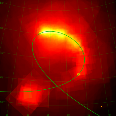
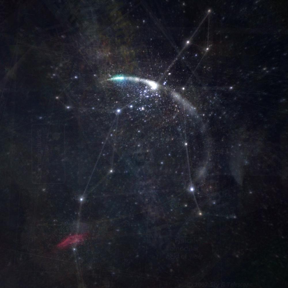
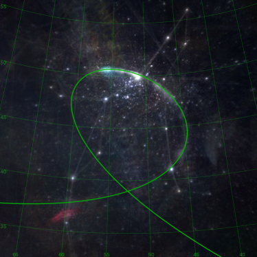
Figure 2: Images that were successfully calibrated by Astrometry.net, aligned in celestial coordinates. We show only the region within about 20 degrees of the comet’s 2007 trajectory; there are 134 images outside the plot area. Top: Total pixel density of the images, with a log stretch. The most heavily imaged point on the sky is covered by 493 images and has a pixel density of over $4$ million pixels per square degree. The colorbar units are pixels per square degree. The right panel shows the same image as the left panel but with a coordinate grid and the trajectory of the JPL ephemeris (Giorgini et al. 1996) for Comet 17P/Holmes. Bottom: Co-added images. The co-added images show the fixed stars because the images have been aligned in celestial coordinates; they show some faint lines joining the stars because some of the images used in this study are diagrams of the constellations rather than plain photographs. The California Nebula (NGC 1499) is visible in the bottom-left of the image because many photographers imaged the conjunction of the comet and nebula (see, for example, Figure 1(1)).