Hydromagnetic Waves in Weakly Ionised Media. I. Basic Theory, and Application to Interstellar Molecular Clouds

Abstract

We present a comprehensive study of MHD waves and instabilities in a weakly ionised system, such as an interstellar molecular cloud. We determine all the critical wavelengths of perturbations across which the sustainable wave modes can change radically (and so can their decay rates), and various instabilities are present or absent. Hence, these critical wavelengths are essential for understanding the effects of MHD waves (or turbulence) on the structure and evolution of molecular clouds. Depending on the angle of propagation relative to the zeroth-order magnetic field and the physical parameters of a model cloud, there are wavelength ranges in which no wave can be sustained as such. Yet, for other directions of propagation or different properties of a model cloud, there may always exist some wave mode(s) at all wavelengths (smaller than the size of the model cloud). For a typical model cloud, magnetically-driven ambipolar diffusion leads to removal of any support against gravity that most short-wavelength waves (or turbulence) may have had, and gravitationally-driven ambipolar diffusion sets in and leads to cloud fragmentation into stellar-size masses, as first suggested by Mouschovias more than three decades ago – a single-stage fragmentation theory of star formation, distinct from the then prevailing hierarchical fragmentation picture. The phase velocities, decay times, and eigenvectors (e.g., the densities and velocities of neutral particles and the plasma, and the three components of the magnetic field) are determined as functions of the wavelength of the disturbances in a mathematically transparent way and are explained physically. Comparison of the results with those of nonlinear analytical or numerical calculations is also presented where appropriate, excellent agreement is found, and confidence in the analytical, linear approach is gained to explore phenomena difficult to study through numerical simulations. Mode splitting (or bifurcation) and mode merging, which are impossible in single-fluid systems for linear perturbations (hence, the term “normal mode” and the principle of superposition), occur naturally in multifluid systems (as do transitions between wave modes without bifurcation) and have profound consequences in the evolution of such systems.

1 Introduction – Background

A typical molecular cloud which has not yet given birth to stars is a cold ($T\simeq 10~{}\rm{K}$) but complex, partially ionised system, in which self-gravitational and magnetic forces are of comparable magnitude, with thermal-pressure forces becoming important at high densities ($\ga 3\times 10^{8}~{}\rm{cm}^{-3}$) or along magnetic field lines. Mouschovias (1976) showed that, barring external disturbances, if the magnetic field were to be frozen in the matter, interstellar clouds that have not yet given birth to stars would remain in magnetohydrostatic (MHS) equilibrium states. However, ambipolar diffusion (the relative motion of neutral particles and charged particles attached to magnetic field lines) is an unavoidable process in partially ionised media. It reveals itself in two distinct ways, depending on whether it is magnetically or gravitationally driven (see discussion in § 4). The two kinds of ambipolar diffusion acting together initiate fragmentation and star formation in molecular clouds (Mouschovias 1987a).

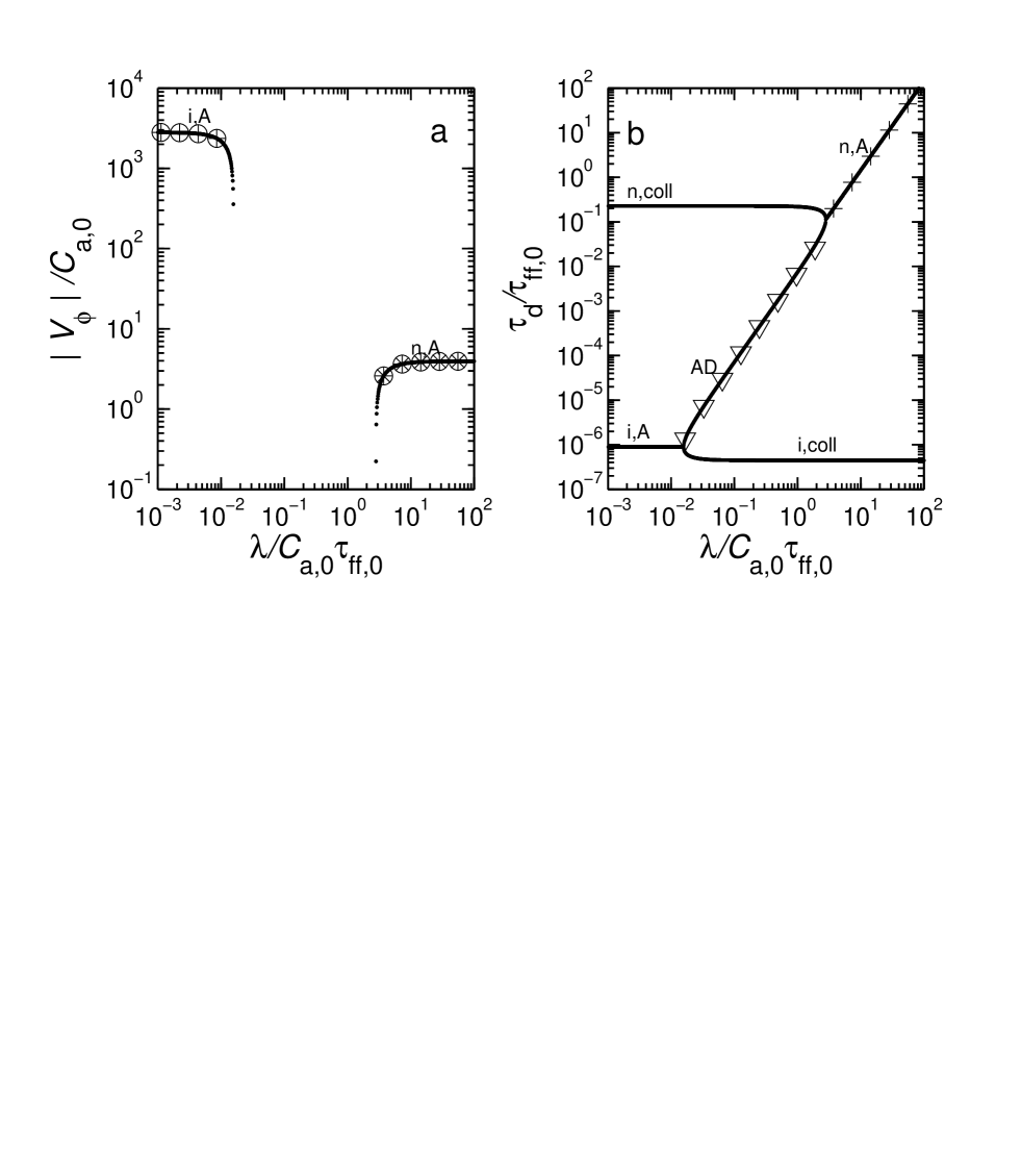
Figure 4: Eigenvalues of transverse modes as functions of wavelength, at an angle of propagation $\theta=0^{\circ}$ with respect to $\mbox{\boldmath$B$}_{0}$. All normalisations are as in Fig. 2. At each wavelength there are four different modes in all: two with motions in the $y$ direction, and two with motions in the $z$ direction. (a) Absolute value of phase velocity, $|{v}_{\phi}|$. Phase velocities resulting from eqs. (26) and (33) are also displayed (circles with interior crosses, and circles with interior asterisks, respectively). (b) Damping timescale $\tau_{{}_{\rm{d}}}$. Also shown are values (downward-facing triangles) calculated from eq. (29a), and values (crosses) calculated from eq. (34a).

In this fragmentation theory, the evolutionary (or fragmentation, or core formation) timescale is the gravitationally-driven ambipolar-diffusion timescale, $\tau_{{}_{\rm{AD}}}$. This does not mean, however, that it takes a time equal to $\tau_{{}_{\rm{AD}}}$ to form stars. The star-formation timescale can be a fraction or a multiple of $\tau_{{}_{\rm{AD}}}$, depending on the mass-to-flux ratio of the parent cloud and the degree to which hydromagnetic waves (HM) contribute to the support of the cloud: the closer to its critical value the mass-to-flux ratio is and/or the greater the contribution of HM waves to cloud support, the faster the evolution and the shorter the star-formation timescale (e.g., see Mouschovias 1987a; Fiedler & Mouschovias 1993, Fig. 9a; Ciolek & Basu 2001; Tassis & Mouschovias 2004, Fig. 4). The collapse retardation factor, $\nu_{{}_{\rm{ff}}}=\tau_{{}_{\rm{ff}}}/\tau_{\rm{ni}}$ (where $\tau_{{}_{\rm{ff}}}$ is the free-fall time and $\tau_{\rm{ni}}$ the neutral-ion collision time), is the factor by which magnetic forces slow down the contraction relative to free-fall. This was a new theory of fragmentation (or core formation), initiated by the decay, due to ambipolar diffusion, of relatively small-wavelength perturbations (Mouschovias 1987a, 1991a).

Magnetic braking operates on a timescale shorter than the ambipolar-diffusion timescale and even the free-fall timescale, and keeps a cloud (or fragment) essentially corotating with the background up to densities $\simeq 10^{4}-10^{6}~{}\rm{cm}^{-3}$ and thus resolves the angular momentum problem of star formation. More specifically, the entire range of periods of binary stars from 10 hr to 100 yr was shown to be accounted for by this self-initiated mode of star formation (Mouschovias 1977). Even single stars and planetary systems become dynamically possible (Mouschovias 1978, 1983).

Star formation, whether self-initiated or triggerred (e.g., by a spiral density wave, or the expansion of an Hii region or a supernova remnant; see review by Woodward 1978) is an inherently nonlinear process. Ambipolar-diffusion$-$initiated star formation has been studied analytically (Mouschovias 1979, 1991a, b) and numerically using adaptive grid techniques in axisymmetric geometry up to densities $\sim 10^{10}~{}\rm{cm}^{-3}$, by which isothermality begins to break down (Fiedler & Mouschovias 1992, 1993; Ciolek & Mouschovias 1993, 1994, 1995; Basu & Mouschovias 1994, 1995a, b). More recently, these calculations were extended into the opaque phases of star formation (Desch & Mouschovias 2001; Tassis & Mouschovias 2007a, b, c; Kunz & Mouschovias 2009, 2010). The key conclusions of the earlier analytical calculations have been verified and numerous new, specific, quantitative predictions have been made, many of which have been confirmed by observations (e.g., see Crutcher et al. 1994; Ciolek & Basu 2000; Chiang et al. 2008; reviews by Mouschovias 1995, 1996). One may nevertheless take a step back from the relatively complicated numerical calculations and ask which results, if any, of the nonlinear simulations can be recovered with a linear analysis. With one’s confidence increased in the validity of the linear approach (within some self-evident limits), one may then make new predictions concerning phenomena that cannot be or have not been included yet in the nonlinear calculations.

The propagation, dissipation, and growth of perturbations in a physical system depends both on the nature of the perturbations and the properties of the system. Hydromagnetic waves (or MHD turbulence) seem to play a significant role in molecular clouds on lengthscales typically greater than $\sim 0.1~{}\rm{pc}$. They have been shown to account quantitatively for the observed supersonic but subAlfvénic spectral linewidths: an observational almost-scatter diagram of linewidth versus size is converted into an almost perfect straight line if plotted in accordance with a theoretical prediction by Mouschovias (1987a), which relates the linewidth, the size, and the magnetic field strength of an observed object (see Mouschovias & Psaltis 1995, Figs. 1 and 2, and update by Mouschovias et al. 2006, Figs. 1 and 2).

Using a linear analysis as a first step in understanding nonlinear phenomena is not, of course, a new idea. Jeans (1928) used it to obtain his famous instability criterion for the collapse of a cloud against thermal-pressure forces. Hardly any astrophysical system exists whose stability with respect to small-amplitude disturbances has not yet been studied by using at least an idealized, mathematically tractable model of the physical system. A magnetically supported molecular cloud, however, defies a simple linear analysis. First, no realistic equilibrium states have been obtained by analytical means. Second, to study the role of ambipolar diffusion in star formation, one must use at least the two-fluid magnetohydrodynamic (MHD) equations governing the motions of the neutral particles and the plasma (ions and electrons). In fact, as shown by Ciolek & Mouschovias (1993), charged (and even neutral) grains play a very significant role in the ambipolar-diffusion$-$initiated protostar formation. One then has to use at least the four-fluid (neutral molecules, plasma, negatively-charged and neutral grains) MHD equations even for a linear analysis to be realistic and relevant to typical molecular clouds. In this paper we use the two-fluid MHD equations to study the propagation, dissipation, and growth of HM waves in an idealized model molecular cloud. In a subsequent paper we consider the effects of the grain fluid(s).

Langer (1978) studied the stability of a model molecular cloud (infinite in extent and uniform in density and magnetic field) with respect to small-amplitude, adiabatic perturbations in the presence of ambipolar diffusion. For propagation along the magnetic field lines, he recovered, as one would expect intuitively, the Jeans dispersion relation and instability in the absence of the magnetic field. He then investigated the wave propagation perpendicular to the field lines. He showed that the Jeans instability is still present, that the critical wavenumber for instability is independent of the magnetic field strength, but that the growth rate depends on both the field strength and the degree of ionisation. Aside from two spurious curves in his Figure 1, which exhibits the growth rate and decay time of some modes, our results for propagation of the low-frequency modes perpendicular to the magnetic field are in agreement with Langer’s – he ignored the high-frequency ion modes. Yet even in this, previously studied case, we offer new analytical expressions and new physical insight and interpretation of the results. Moreover, we present not only the eigenvalues (frequencies or, equivalently, phase velocities) as functions of wavelength but the eigenvectors as well (i.e., material velocities, densities, magnetic-field components, etc.). We also study propagation at arbitrary angles with respect to the magnetic field, and we offer a thorough discussion of the wave modes, not just the ambipolar-diffusion–induced instability.

Pudritz (1990) revisited Langer’s problem (with the minor difference of considering isothermal perturbations) but introduced a new effect: he assumed that there exists a power-law spectrum of small-amplitude waves, and then he studied the effect that this spectrum has on the ambipolar-diffusion–induced, Jeans-like instability. He concluded that the slope of the spectrum (considered as a function of wavelength) has an important effect on the growth rate of the instability; the steeper the spectrum, the greater the growth rate. (The growth rate of gravitationally-driven ambipolar diffusion, however, cannot possibly exceed the free-fall rate.)

Several other papers have appeared in print since 1990, studying different aspects of weakly ionised systems, focusing usually on the stability of certain MHD modes or shocks, especially as it may relate to the formation of structures in molecular clouds and/or on the effect of the grain fluid(s) on the allowable wave modes or shocks (e.g., Wardle 1990; Balsara 1996; Zweibel 1998; Kamaya & Nishi 1998, 2000; Mamun & Shukla 2001; Cramer et al. 2001; Falle & Hartquist 2002; Tytarenko et al. 2002; Zweibel 2002; Ciolek et al. 2004; Lim et al. 2005; Oishi & Mac Low 2006; Roberge & Ciolek 2007; van Loo et al. 2008; Li & Houde 2008). In this paper we present a general theory of the propagation, dissipation and growth of MHD waves in partially ionised media in three dimensions, with emphasis on mathematical transparency of the formulation and analytical solution of the problem, the physical understanding and interpretation of all modes, including their eigenvectors, the many critical wavelengths that exist and which separate regimes dominated by different waves or instabilities, and on specific features relevant to the evolution of molecular clouds. As mentioned above, even when a particular result agrees with previous work, we offer new insight into its physical understanding.

In § 2 we present the equations governing the behaviour of a weakly ionised, magnetic, self-gravitating interstellar cloud. The equations are linearised, Fourier-analyzed, and put in dimensionless form. The free parameters of the problem are identified, their physical meaning explained, and their typical values given. The different hydromagnetic modes and their dependence on wavelength for different directions of propagation relative to the magnetic field are calculated and explained physically in § 3. Analytical expressions for the phase velocities, damping timescales, growth timescales, including critical or cutoff wavelengths, are also obtained. A physical discussion of the eigenvectors is an integral part of this presentation. Section 4 summarizes some of the results and their relevance to the formation of protostellar fragments (or cores) and to other observable phenomena. It also gives in two Tables all the critical wavelengths and the ranges of wavelengths in which different modes can exist in molecular clouds, for propagation parallel, perpendicular, and at arbitrary angles with respect to the magnetic field.

2 FORMULATION OF THE PROBLEM

2.1 Basic Equations

We consider a weakly ionised medium (e.g., an interstellar molecular cloud) consisting of neutral particles ($\rm{H}_{2}$ with a $20\%$ helium abundance by number; subscript n), electrons, and singly-charged positive ions (subscript i). For specificity we assume that the ions are molecular ions (such as $\rm{HCO}^{+}$); for the densities of interest in this paper ($\sim 10^{3}\,\rm{cm}^{-3}$), this is sufficient since atomic ions (such as $\rm{Na}^{+}$ or $\rm{Mg}^{+}$) are less abundant (a result of depletion of metals in dense clouds) and, in any case, they have masses comparable to that of $\rm{HCO}^{+}$ (for more detailed treatments of the chemistry, see Ciolek & Mouschovias 1995, 1998, or the appendix of Mouschovias & Ciolek 1999). Interstellar grains, which have been shown to have significant effects on the formation and contraction of protostellar cores (Ciolek & Mouschovias 1993, 1994, 1995) and in the opaque phase of star formation (Tassis & Mouschovias 2007a, b, c; Kunz & Mouschovias 2009, 2010) are neglected in this analysis; they are accounted for in a subsequent paper.

The magnetohydrodynamic (MHD) equations governing the evolution of the above two-fluid system are

$$\frac{\partial\rho_{\rm n}}{\partial t}+\nabla\cdot\left(\rho_{\rm n}\mbox{\boldmath$v$}_{\rm n}\right) = 0,$$ (1a)

$$\frac{\partial\rho_{\rm i}}{\partial t}+\nabla\cdot\left(\rho_{\rm i}\mbox{\boldmath$v$}_{\rm i}\right) = m_{\rm{i}}\zeta_{{}_{\rm{CR}}}\frac{\rho_{\rm n}}{\mu m_{\rm H}}-\frac{\alpha_{\rm{dr}}}{m_{\rm{i}}}\rho_{\rm i}^{2},$$ (1b)

$$\rho_{\rm n}\left[\frac{d}{dt}\right]_{\rm n}\mbox{\boldmath$v$}_{\rm n} = -\nabla P_{\rm n}-\rho_{\rm n}\nabla\psi-\frac{\rho_{\rm n}}{\tau_{\rm{ni}}}\left(\mbox{\boldmath$v$}_{\rm n}-\mbox{\boldmath$v$}_{\rm i}\right),$$ (1c)

$$\rho_{\rm i}\left[\frac{d}{dt}\right]_{\rm i}\mbox{\boldmath$v$}_{\rm i} = \frac{\left(\nabla\mbox{\boldmath$\times$}\mbox{\boldmath$B$}\right)\mbox{\boldmath$\times$}\mbox{\boldmath$B$}}{4\pi}-\frac{\rho_{\rm i}}{\tau_{\rm{in}}}\left(\mbox{\boldmath$v$}_{\rm i}-\mbox{\boldmath$v$}_{\rm n}\right),$$ (1d)

$$\frac{k_{\rm B}}{\mu m_{\rm H}}\left\{\frac{\rho_{\rm n}}{\gamma-1}\left[\frac{d}{dt}\right]_{\rm n}T-T\left[\frac{d}{dt}\right]_{\rm n}\rho_{\rm n}\right\} = \Gamma_{\rm n}-\Lambda_{\rm n},$$ (1e)

$$\frac{\partial\mbox{\boldmath$B$}}{\partial t} = \nabla\mbox{\boldmath$\times$}\left(\mbox{\boldmath$v$}_{\rm i}\mbox{\boldmath$\times$}\mbox{\boldmath$B$}\right),$$ (1f)

$$P_{\rm n} = \rho_{\rm n}\frac{k_{\rm B}T}{\mu m_{\rm H}},$$ (1g)

$$\nabla^{2}\psi = 4\pi G\rho_{\rm n},$$ (1h)

$$\nabla\cdot\mbox{\boldmath$B$} = 0,$$ (1i)

where $\rho_{\alpha}$ and $\mbox{\boldmath$v$}_{\alpha}$ are, respectively, the density and velocity of species $\alpha$,

$$\left[\frac{d}{dt}\right]_{\alpha}=\frac{\partial}{\partial t}+\mbox{\boldmath$v$}_{\alpha}\cdot\nabla$$ (2)

is the time-derivative comoving with species $\alpha$, $\psi$ the gravitational potential, $P_{\rm n}$ the neutral pressure, $B$ the magnetic field, $T$ the temperature, $\Gamma_{\rm n}$ and $\Lambda_{\rm n}$ the heating and cooling rates (per unit volume) of the neutral gas, and

$$\tau_{\rm{ni}} = 1.4\frac{m_{\rm{i}}+m_{\rm{H}_{2}}}{m_{\rm{i}}}\frac{1}{n_{\rm i}{\langle\sigma w\rangle}_{\rm{i}\rm{H}_{2}}},$$ (3a)

$$\tau_{\rm{in}} = 1.4\frac{m_{\rm{i}}+m_{\rm{H}_{2}}}{\mu m_{\rm H}}\frac{1}{n_{\rm{n}}{\langle\sigma w\rangle}_{\rm{i}\rm{H}_{2}}},$$ (3b)

the neutral-ion and ion-neutral mean collision (i.e., momentum-exchange) times. The quantity $G$ is the universal gravitational constant, and $k_{\rm B}$ is Boltzmann’s constant; $\mu$ is the mean mass of a neutral particle in units of the atomic-hydrogen mass and is equal to 2.33 for a $\rm{H}_{2}$ gas with a $20\%$ helium abundance by number. The quantities $\zeta_{{}_{\rm{CR}}}$ and $\alpha_{\rm{dr}}$ in the ion mass continuity equation (1b) are, respectively, the cosmic-ray ionisation rate and the coefficient for dissociative recombination of molecular ions and electrons (in $\rm{cm}^{3}~{}\rm{s}^{-1}$). In writing equation (1b), we have used the condition of local charge neutrality $e(n_{\rm i}-n_{\rm e})=0$, where $n_{\rm i}$ and $n_{\rm e}$ are, respectively, the number densities of ions and electrons. We may use the assumption of local charge neutrality because the various HM modes of interest here have frequencies much smaller than the electron plasma frequency $\omega_{\rm{p,e}}=(4\pi n_{\rm e}e^{2}/m_{\rm e})^{1/2}=(4\pi x_{\rm e}n_{\rm{n}}e^{2}/m_{\rm e})^{1/2}=5.64\times 10^{2}~{}(x_{\rm e}/10^{-7})^{1/2}(n_{\rm{n}}/10^{3}~{}\rm{cm}^{-3})^{1/2}~{}\rm{s}^{-1}$ (where $x_{\rm e}=n_{\rm e}/n_{\rm{n}}$ is the abundance of electrons relative to the neutrals, and is equal to the degree of ionisation for weakly-ionised systems); hence, any excess charge density is quickly shielded by the mobile electrons, so that $n_{\rm e}=n_{\rm i}$ for timescales $\ga\omega_{\rm{p,e}}^{-1}$. Since we neglect the effects of grains in this paper, capture of ions onto grains is not included on the right-hand side of equation (1b) as a sink term for ions.

Heat conduction and viscosity are not important for the densities and lengthscales of interest ($n_{\rm{n}}\simeq 10^{2}-10^{5}~{}\rm{cm}^{-3}$, $L\simeq 10^{-3}-10^{1}~{}\rm{pc}$), and are therefore ignored as possible sources of heating/cooling in the model clouds. (Note that the left-hand side of equation [1e] is equal to $\rho_{\rm n}T[d/dt]_{\rm n}S$, where $S$ is the entropy per gram of matter.)

Because $\rho_{\rm n}\gg\rho_{\rm e},~{}\rho_{\rm i}$, we include only the neutral density as a source term in Poisson’s equation (1h). Similarly, the gravitational and thermal-pressure forces (per unit volume) on the plasma (ions and electrons) have been neglected in the plasma force equation (1d). One can easily show that, for the physical conditions in typical molecular clouds, they are completely negligible in comparison to the magnetic force exerted on the plasma, except in a direction almost exactly parallel to the magnetic field. Ignoring them parallel to the magnetic field implies that we are neglecting the ion acoustic waves and the (extremely long-wavelength) Jeans instability in the ions.

The quantity ${\langle\sigma w\rangle}_{\rm{i}\rm{H}_{2}}$ in equations (3a) and (3b) is the elastic collision rate between ions and neutrals. For $\rm{HCO}^{+}-\rm{H}_{2}$ collisions, ${\langle\sigma w\rangle}_{\rm{i}\rm{H}_{2}}=1.69\times 10^{-9}~{}\rm{cm}^{3}~{}\rm{s}^{-1}$ (McDaniel & Mason 1973). The factor 1.4 in equations (3a) and (3b) accounts for the inertial effect of He on the motion of the neutrals (for a discussion, see § 2.1 of Mouschovias & Ciolek 1999).

2.2 Linear System

To investigate the propagation, dissipation, and growth of HM waves in molecular clouds, we follow the original analysis by Jeans (1928; see also Spitzer 1978, § 13.3a; and Binney & Tremaine 1987, § 5.1), and assume that the zeroth-order state is uniform, static (i.e., $\mbox{\boldmath$v$}_{\alpha}=0$), and in equilibrium. We consider only adiabatic perturbations; therefore, the net heating rate ($\Gamma_{\rm n}-\Lambda_{\rm n}$) on the right-hand side of equation (1e) vanishes.

We write any scalar quantity or component of a vector $q_{\rm{tot}}(\mbox{\boldmath$r$},t)$ in the form $q_{\rm{tot}}(\mbox{\boldmath$r$},t)=q_{0}+q(\mbox{\boldmath$r$},t)$, where $q_{0}$ refers to the zeroth-order state, and the first-order quantity $q$ satisfies the condition $|q|\ll|q_{0}|$. We thus obtain from equations (1a) - (1i) the linearised system

$$\frac{\partial\rho_{\rm n}}{\partial t} = -\rho_{\rm n,0}\left(\nabla\cdot\mbox{\boldmath$v$}_{\rm n}\right),$$ (4a)

$$\frac{\partial\rho_{\rm i}}{\partial t} = -\rho_{\rm i,0}\left(\nabla\cdot\mbox{\boldmath$v$}_{\rm i}\right)+\frac{\rho_{\rm i,0}}{\mu m_{\rm H}}x_{\rm i,0}\alpha_{\rm{dr}}\rho_{\rm n}-2\frac{\rho_{\rm i,0}}{m_{\rm{i}}}\alpha_{\rm{dr}}\rho_{\rm i},$$ (4b)

$$\rho_{\rm n,0}\frac{\partial\mbox{\boldmath$v$}_{\rm n}}{\partial t} = -\nabla P_{\rm n}-\rho_{\rm n,0}\nabla\psi-\frac{\rho_{\rm n,0}}{\tau_{{\rm{ni,0}}}}\left(\mbox{\boldmath$v$}_{\rm n}-\mbox{\boldmath$v$}_{\rm i}\right),$$ (4c)

$$\rho_{\rm i,0}\frac{\partial\mbox{\boldmath$v$}_{\rm i}}{\partial t} = \frac{\left(\nabla\mbox{\boldmath$\times$}\mbox{\boldmath$B$}\right)\mbox{\boldmath$\times$}\mbox{\boldmath$B$}_{0}}{4\pi}-\frac{\rho_{\rm i,0}}{\tau_{{\rm{in,0}}}}\left(\mbox{\boldmath$v$}_{\rm i}-\mbox{\boldmath$v$}_{\rm n}\right),$$ (4d)

$$\frac{1}{T_{0}}\frac{\partial T}{\partial t} = \left(\gamma-1\right)\frac{1}{\rho_{\rm n,0}}\frac{\partial\rho_{\rm n}}{\partial t},$$ (4e)

$$\frac{\partial\mbox{\boldmath$B$}}{\partial t} = \nabla\mbox{\boldmath$\times$}\left(\mbox{\boldmath$v$}_{\rm i}\mbox{\boldmath$\times$}\mbox{\boldmath$B$}_{0}\right),$$ (4f)

$$\frac{P_{\rm n}}{P_{\rm{n,0}}} = \frac{\rho_{\rm n}}{\rho_{\rm n,0}}+\frac{T}{T_{0}},$$ (4g)

$$\nabla^{2}\psi = 4\pi G\rho_{\rm n},$$ (4h)

$$\nabla\cdot\mbox{\boldmath$B$} = 0.$$ (4i)

Equation (4b) has been simplified by using the relation

$$\zeta_{{}_{\rm{CR}}}\frac{\rho_{\rm n,0}}{\mu m_{\rm H}}=\alpha_{\rm{dr}}\left(\frac{\rho_{\rm i,0}}{m_{\rm{i}}}\right)^{2},$$ (5)

which expresses equilibrium of the ion density in the zeroth-order state, as a result of balance between the rate of creation of ions from ionisation of neutral matter by high-energy ($E\ga 100~{}\rm{MeV}$) cosmic rays and the rate of destruction of ions by electron$-$molecular-ion dissociative recombinations. This relation allowed us to replace $\zeta_{{}_{\rm{CR}}}$ by $\alpha_{\rm{dr}}(\rho_{\rm i,0}/m_{\rm{i}})^{2}(\mu m_{\rm H}/\rho_{\rm n,0})$ in equation (4b). The quantity $x_{\rm i,0}\equiv n_{\rm{i,0}}/n_{\rm{n,0}}$ in equation (4b) is the degree of ionisation (where $n_{\rm{i,0}}$ and $n_{\rm{n,0}}$ are the number densities of ions and neutrals in the unperturbed state). For an ideal gas (with only translational degrees of freedom), $\gamma=5/3$ in equation (4e).

We seek plane-wave solutions of the form $q(\mbox{\boldmath$r$},t)=\overline{q}\exp(i\mbox{\boldmath$k$}\cdot\mbox{\boldmath$r$}-i\omega t)$, where $k$ is the propagation vector, $\omega$ the frequency, and $\overline{q}$ the amplitude (in general, complex) of the perturbation. Equations (4a) - (4i) reduce to

$$\omega\rho_{\rm n} = \rho_{\rm n,0}\mbox{\boldmath$k$}\cdot\mbox{\boldmath$v$}_{\rm n},$$ (6a)

$$\omega\rho_{\rm i} = \rho_{\rm i,0}\mbox{\boldmath$k$}\cdot\mbox{\boldmath$v$}_{\rm i}+i\frac{\rho_{\rm i,0}}{\mu m_{\rm H}}x_{\rm i,0}\alpha_{\rm{dr}}\rho_{\rm n}-i2\frac{\rho_{\rm i,0}}{m_{\rm{i}}}\alpha_{\rm{dr}}\rho_{\rm i},$$ (6b)

$$\omega\mbox{\boldmath$v$}_{\rm n} = \left(C_{\rm{a},0}^{2}k-\frac{1}{\tau_{{}_{\rm{ff,0}}}^{2}k}\right)\frac{\rho_{\rm n}}{\rho_{\rm n,0}}\frac{\mbox{\boldmath$k$}}{k}-\frac{i}{\tau_{{\rm{ni,0}}}}\mbox{\boldmath$v$}_{\rm n}+\frac{i}{\tau_{{\rm{ni,0}}}}\mbox{\boldmath$v$}_{\rm i},$$ (6c)

$$\omega\mbox{\boldmath$v$}_{\rm i} = -\frac{\left(\mbox{\boldmath$k$}\mbox{\boldmath$\times$}\mbox{\boldmath$B$}\right)\mbox{\boldmath$\times$}\mbox{\boldmath$B$}_{0}}{4\pi\rho_{\rm i,0}}+\frac{i}{\tau_{{\rm{in,0}}}}\mbox{\boldmath$v$}_{\rm n}-\frac{i}{\tau_{{\rm{in,0}}}}\mbox{\boldmath$v$}_{\rm i},$$ (6d)

$$\omega\mbox{\boldmath$B$} = -\mbox{\boldmath$k$}\mbox{\boldmath$\times$}\left(\mbox{\boldmath$v$}_{\rm i}\mbox{\boldmath$\times$}\mbox{\boldmath$B$}_{0}\right),$$ (6e)

$$\mbox{\boldmath$k$}\cdot\mbox{\boldmath$B$} = 0,$$ (6f)

where

$$C_{\rm{a},0}\equiv\left(\frac{\gamma P_{\rm{n,0}}}{\rho_{\rm n,0}}\right)^{1/2}=\left(\frac{\gamma k_{\rm B}T_{0}}{\mu m_{\rm H}}\right)^{1/2}$$ (7)

is the adiabatic speed of sound in the neutrals, and

$$\tau_{{}_{\rm{ff,0}}}\equiv\left(4\pi G\rho_{\rm n,0}\right)^{-1/2}$$ (8)

is the (one-dimensional) neutral free-fall timescale. The quantities $T$, $P_{\rm n}$, and $\psi$ have been eliminated by using equations (4e), (4g), and (4h), respectively.

2.3 The Dimensionless Problem

We put equations (6a) - (6f) in dimensionless form by adopting $\rho_{\rm n,0}$, $B_{0}$, $\tau_{{}_{\rm{ff,0}}}$, and $C_{\rm{a},0}$ as units of density, magnetic field strength, time, and speed, respectively. The implied unit of length is $C_{\rm{a},0}\tau_{{}_{\rm{ff,0}}}$, which is proportional to the one-dimensional thermal Jeans lengthscale $\lambda_{\rm{J,th}}$ (see § 3.1.1). For convenience, we adopt a cartesian coordinate system such that the propagation vector $k$ is in the $x$-direction and the zeroth-order magnetic field $\mbox{\boldmath$B$}_{0}$ is in the $(x,z)$-plane at an angle $\theta$ with respect to $k$ (see Fig. 1). Then the three unit vectors are

$$\hat{\mbox{\boldmath$e$}}_{x} \equiv \frac{\mbox{\boldmath$k$}}{k},$$ (9a)

$$\hat{\mbox{\boldmath$e$}}_{y} \equiv \frac{\mbox{\boldmath$B$}_{0}\mbox{\boldmath$\times$}\mbox{\boldmath$k$}}{|\mbox{\boldmath$B$}_{0}\mbox{\boldmath$\times$}\mbox{\boldmath$k$}|},$$ (9b)

$$\hat{\mbox{\boldmath$e$}}_{z} \equiv \hat{\mbox{\boldmath$e$}}_{x}\mbox{\boldmath$\times$}\hat{\mbox{\boldmath$e$}}_{y}.$$ (9c)

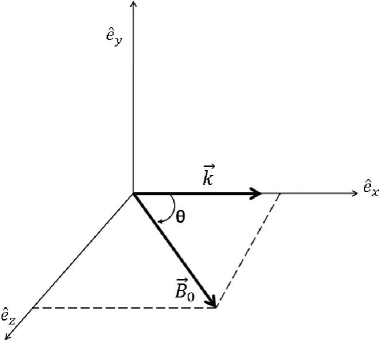
Figure 1: Coordinate system used in analysing the linearised hydromagnetic equations. The $x$-axis is aligned with the propagation vector $k$, and the magnetic field $\mbox{\boldmath$B$}_{0}$ is in the $(x,z)$-plane at an angle $\theta$ with respect to $k$ (see eqs. [9a] - [9c]).

One may write $\mbox{\boldmath$B$}_{0}=\hat{\mbox{\boldmath$e$}}_{x}B_{0}\cos\theta+\hat{\mbox{\boldmath$e$}}_{z}B_{0}\sin\theta$, and the dimensionless form of equations (6a) - (6f) can be written in component form as

$$\tilde{\omega}\tilde{\rho}_{\rm n} = \tilde{k}\tilde{v}_{{\rm n},x},$$ (10a)

$$\tilde{\omega}\tilde{\rho}_{\rm i} = \tilde{\rho}_{\rm{i,0}}\tilde{k}\tilde{v}_{{\rm i},x}+i\tilde{\rho}_{\rm{i,0}}^{2}\tilde{\alpha}_{\rm{m,dr}}\tilde{\rho}_{\rm n}-i2\tilde{\rho}_{\rm{i,0}}\tilde{\alpha}_{\rm{m,dr}}\tilde{\rho}_{\rm i},$$ (10b)

$$\tilde{\omega}\tilde{v}_{{\rm n},x} = \left(\tilde{k}-\frac{1}{\tilde{k}}\right)\tilde{\rho}_{\rm n}-\frac{i}{\tilde{\tau}_{{\rm{ni,0}}}}\tilde{v}_{{\rm n},x}+\frac{i}{\tilde{\tau}_{{\rm{ni,0}}}}\tilde{v}_{{\rm i},x},$$ (10c)

$$\tilde{\omega}\tilde{v}_{{\rm i},x} = \frac{i}{\tilde{\tau}_{{\rm{in,0}}}}\tilde{v}_{{\rm n},x}-\frac{i}{\tilde{\tau}_{{\rm{in,0}}}}\tilde{v}_{{\rm i},x}+\tilde{v}_{\rm{A,i,0}}^{2}\tilde{k}\tilde{B}_{z}\sin\theta,$$ (10d)

$$\tilde{\omega}\tilde{B}_{x} = 0,$$ (10e)

$$\tilde{\omega}\tilde{v}_{{\rm n},y} = -\frac{i}{\tilde{\tau}_{{\rm{ni,0}}}}\tilde{v}_{{\rm n},y}+\frac{i}{\tilde{\tau}_{{\rm{ni,0}}}}\tilde{v}_{{\rm i},y},$$ (10f)

$$\tilde{\omega}\tilde{v}_{{\rm i},y} = \frac{i}{\tilde{\tau}_{{\rm{in,0}}}}\tilde{v}_{{\rm n},y}-\frac{i}{\tilde{\tau}_{{\rm{in,0}}}}\tilde{v}_{{\rm i},y}-\tilde{v}_{\rm{A,i,0}}^{2}\tilde{k}\tilde{B}_{y}\cos\theta,$$ (10g)

$$\tilde{\omega}\tilde{B}_{y} = -\tilde{k}\tilde{v}_{{\rm i},y}\cos\theta,$$ (10h)

$$\tilde{\omega}\tilde{v}_{{\rm n},z} = -\frac{i}{\tilde{\tau}_{{\rm{ni,0}}}}\tilde{v}_{{\rm n},z}+\frac{i}{\tilde{\tau}_{{\rm{ni,0}}}}\tilde{v}_{{\rm i},z},$$ (10i)

$$\tilde{\omega}\tilde{v}_{{\rm i},z} = \frac{i}{\tilde{\tau}_{{\rm{in,0}}}}\tilde{v}_{{\rm n},z}-\frac{i}{\tilde{\tau}_{{\rm{in,0}}}}\tilde{v}_{{\rm i},z}-\tilde{v}_{\rm{A,i,0}}^{2}\tilde{k}\tilde{B}_{z}\cos\theta,$$ (10j)

$$\tilde{\omega}\tilde{B}_{z} = \tilde{k}\tilde{v}_{{\rm i},x}\sin\theta-\tilde{k}\tilde{v}_{{\rm i},z}\cos\theta,$$ (10k)

$$\tilde{k}\tilde{B}_{x} = 0.$$ (10l)

Note that equation (10l) is redundant in that it gives the same information as equation (10e), namely, that there cannot be a nonvanishing component of the perturbed magnetic field in the direction of propagation.

The dimensionless free parameters appearing in equations (10a) - (10l) are given by

$$\tilde{\tau}_{{\rm{ni,0}}} \equiv \frac{\tau_{{\rm{ni,0}}}}{\tau_{{}_{\rm{ff,0}}}}=0.506\left(\frac{10^{-7}}{x_{\rm i,0}}\right)\left(\frac{10^{3}~{}{\rm{cm}^{-3}}}{n_{\rm{n,0}}}\right)^{1/2},$$ (11a)

$$\tilde{\tau}_{{\rm{in,0}}} \equiv \frac{\tau_{{\rm{in,0}}}}{\tau_{{}_{\rm{ff,0}}}}=6.29\times 10^{-7}\left(\frac{10^{3}{~{}\rm{cm}^{-3}}}{n_{\rm{n,0}}}\right)^{1/2},$$ (11b)

$$\tilde{v}_{\rm{A,i,0}} \equiv \frac{v_{\rm{A,i,0}}}{C_{\rm{a},0}}=5.00\times 10^{3}\left(\frac{B_{0}}{30~{}\mu\rm{G}}\right)\left(\frac{10^{-7}}{x_{\rm i,0}}\right)^{1/2}\left(\frac{10~{}{\rm K}}{T}\right)^{1/2}\left(\frac{10^{3}~{}{\rm{cm}^{-3}}}{n_{\rm{n,0}}}\right)^{1/2},$$ (11c)

$$\tilde{\alpha}_{\rm{m,dr}} \equiv \frac{\alpha_{\rm{dr}}}{m_{\rm{i}}}\rho_{\rm n,0}\tau_{{}_{\rm{ff,0}}}=1.41\times 10^{9}\left(\frac{\alpha_{\rm{dr}}}{10^{-6}~{}\rm{cm}^{3}~{}\rm{s}^{-1}}\right)\left(\frac{n_{\rm{n,0}}}{10^{3}~{}\rm{cm}^{-3}}\right)^{1/2}\left(\frac{29~{}{\rm{amu}}}{m_{\rm{i}}}\right);$$ (11d)

they represent, respectively, the neutral-ion collision time, the ion-neutral collision time, the ion Alfvén speed $$v_{\rm{A,i,0}}=B_{0}/(4\pi\rho_{\rm i,0})^{1/2} - \mu=2.33 \gamma=5/3 \rm{HCO}^{+} m_{\rm{i}} \mu m_{\rm H} \tilde{\rho}_{\rm{i,0}} \tilde{\zeta}_{{}_{\rm{CR}}} \tilde{\tau}_{{\rm{in,0}}}/\tilde{\tau}_{{\rm{ni,0}}} {\tilde{\rho}_{\rm{i,0}}}^{2}\tilde{\alpha}_{\rm{m,dr}} \tilde{\alpha}_{\rm{m,dr}}$$, and the electronmolecular-ion dissociative recombination rate per unit ion mass. In evaluating the numerical constants in equations (11a) - (11d) we have used and ; we have also normalized the ion mass to that of (= 29 amu). For any given ion mass and mean mass per neutral particle (in units of ), the ion mass fraction and the cosmic-ray ionisation rate are not free parameters in the problem; the former is determined by the ratio and the latter by the product , where is the dimensionless dissociative-recombination coefficient for molecular ions.

We note that $\tilde{\tau}_{{\rm{ni,0}}}=1/\nu_{\rm{ff},0}$, where $\nu_{\rm{ff},0}$ is the collapse retardation factor, which is a parameter that measures the effectiveness with which magnetic forces are transmitted to the neutrals via neutral-ion collisions (Mouschovias 1982), and appears naturally in the timescale for the formation of protostellar cores by ambipolar diffusion (e.g., see reviews by Mouschovias 1987a, § 2.2.5; 1987b, § 3.4; 1991b, § 2.3.1; and discussions in Fiedler & Mouschovias 1992, 1993; Ciolek & Mouschovias 1993, 1994, 1995; Basu & Mouschovias 1994, 1995). It is essentially the factor by which ambipolar diffusion in a magnetically supported cloud retards the formation and contraction of a protostellar fragment (or core) relative to free fall up to the stage at which the mass-to-flux ratio exceeds the critical value for collapse. It is discussed further in § 3.2.1.

Equations (10a) - (10k) govern the behaviour of small-amplitude disturbances in a weakly ionised cloud; they (without eq. [10e]) form a $10\times 10$ homogeneous system. In general, the dispersion relation $\tilde{\omega}(\tilde{k})$ can be obtained by setting the determinant of the coefficients equal to zero. To each root (eigenvalue) of the dispersion relation there corresponds an eigenvector (or “mode”), whose components are the dependent variables appearing in equations (10a) - (10k). (Note that, once the dependent variables in eqs. [10a] - [10k] are known, one may use eqs. [4e], [4g], and [4h] to solve for the perturbed quantities $T$, $P_{\rm n}$, and $\psi$, respectively.) Since, in general, $\tilde{\omega}$ is complex, modes with $\rm{Im}\{\tilde{\omega}\}<0$ decay and those with $\rm{Im}\{\tilde{\omega}\}>0$ grow exponentially in time. In what follows we investigate the propagation, dissipation, and growth of the allowable HM modes in typical interstellar molecular clouds.

3 SOLUTION, PHYSICAL INTERPRETATION, AND APPLICATIONS

For specificity, we consider a representative molecular cloud of density $n_{\rm{n,0}}=2\times 10^{3}~{}\rm{cm}^{-3}$, magnetic field strength $B_{0}=30~{}\mu\rm{G}$, temperature $T=10~{}\rm{K}$, dissociative recombination rate $\alpha_{\rm{dr}}=10^{-6}~{}\rm{cm}^{3}~{}{\rm s}^{-1}$, and cosmic-ray ionisation rate $\zeta_{{}_{\rm{CR}}}=5\times 10^{-17}~{}\rm{s}^{-1}$, implying a degree of ionisation $x_{\rm i,0}=1.58\times 10^{-7}$ (and, hence, ion mass fraction $\tilde{\rho}_{\rm{i,0}}=1.97\times 10^{-6}$). The unit of time $\tau_{{}_{\rm{ff,0}}}$ (see eq. [8]) for this model is equal to $3.92\times 10^{5}~{}\rm{yr}$, and the unit of speed is $C_{\rm{a},0}=0.243~{}\rm{km}~{}\rm{s}^{-1}$ (see eq. [7]). Hence, the unit of length is $C_{\rm{a},0}\tau_{{}_{\rm{ff,0}}}=9.72\times 10^{-2}~{}\rm{pc}$. The four (dimensionless) free parameters of the problem (see eqs. [11a] - [11d]) are: the ion-neutral collision time $\tilde{\tau}_{{\rm{in,0}}}=4.45\times 10^{-7}$, the neutral-ion collision time $\tilde{\tau}_{{\rm{ni,0}}}=0.226$, the Alfvén speed in the ions $\tilde{v}_{\rm{A,i,0}}=2.81\times 10^{3}$, and the dissociative-recombination coefficient $\tilde{\alpha}_{\rm{m,dr}}=1.99\times 10^{9}$. (These imply a dimensionless cosmic-ray ionisation rate $\tilde{\zeta}_{{}_{\rm{CR}}}=6.19\times 10^{-4}$.)

In the following subsections we present the solutions for propagation along ($\theta=0^{\circ}$), perpendicular ($\theta=90^{\circ}$), and at intermediate angles ($\theta=45^{\circ}$, $10^{\circ}$, and $80^{\circ}$) with respect to the unperturbed magnetic field $\mbox{\boldmath$B$}_{0}$ (see Fig. 1). We use the velocity vector $v$ in relation to $k$ as defining the polarisation of each wave mode. Modes that have only $\tilde{v}_{{\rm n},x}$, $\tilde{v}_{{\rm i},x}\neq 0$ are said to be longitudinally polarised; it follows from equation (10a) that these modes are compressible, i.e., $\tilde{\rho}_{\rm n}\neq 0$. Modes that have $\tilde{v}_{{\rm n},x}$, $\tilde{v}_{{\rm i},x}=0$ are said to be transversely polarised; they are incompressible, i.e., $\tilde{\rho}_{\rm n}=0$. Note in what follows that, since the thermal pressure in the plasma has been neglected, no ion sound waves are present.

3.1 Propagation Along $\mbox{\boldmath$B$}_{0}$ ($\mbox{\boldmath$k$}\parallel\mbox{\boldmath$B$}_{0}$)

For $\theta=0^{\circ}$, equations [10a] - [10k] become uncoupled in the three mutually orthogonal directions $\hat{\mbox{\boldmath$e$}}_{x}$, $\hat{\mbox{\boldmath$e$}}_{y}$, and $\hat{\mbox{\boldmath$e$}}_{z}$. The modes polarised in the $x$-direction are given by (see eqs. [10a] - [10d])

$$\tilde{\omega}\tilde{\rho}_{\rm n} = \tilde{k}\tilde{v}_{{\rm n},x},$$ (12a)

$$\tilde{\omega}\tilde{\rho}_{\rm i} = \tilde{\rho}_{\rm{i,0}}\tilde{k}\tilde{v}_{{\rm i},x}+i\tilde{\rho}_{\rm{i,0}}^{2}\tilde{\alpha}_{\rm{m,dr}}\tilde{\rho}_{\rm n}-i2\tilde{\rho}_{\rm{i,0}}\tilde{\alpha}_{\rm{m,dr}}\tilde{\rho}_{\rm i},$$ (12b)

$$\tilde{\omega}\tilde{v}_{{\rm n},x} = \left(\tilde{k}-\frac{1}{\tilde{k}}\right)\tilde{\rho}_{\rm n}-\frac{i}{\tilde{\tau}_{{\rm{ni,0}}}}\tilde{v}_{{\rm n},x}+\frac{i}{\tilde{\tau}_{{\rm{ni,0}}}}\tilde{v}_{{\rm i},x},$$ (12c)

$$\tilde{\omega}\tilde{v}_{{\rm i},x} = \frac{i}{\tilde{\tau}_{{\rm{in,0}}}}\tilde{v}_{{\rm n},x}-\frac{i}{\tilde{\tau}_{{\rm{in,0}}}}\tilde{v}_{{\rm i},x}.$$ (12d)

Equations (10f) - (10h) yield for the modes with motions in the $y$-direction

$$\tilde{\omega}\tilde{v}_{{\rm n},y} = -\frac{i}{\tilde{\tau}_{{\rm{ni,0}}}}\tilde{v}_{{\rm n},y}+\frac{i}{\tilde{\tau}_{{\rm{ni,0}}}}\tilde{v}_{{\rm i},y},$$ (13a)

$$\tilde{\omega}\tilde{v}_{{\rm i},y} = \frac{i}{\tilde{\tau}_{{\rm{in,0}}}}\tilde{v}_{{\rm n},y}-\frac{i}{\tilde{\tau}_{{\rm{in,0}}}}\tilde{v}_{{\rm i},y}-\tilde{v}_{\rm{A,i,0}}^{2}\tilde{k}\tilde{B}_{y},$$ (13b)

$$\tilde{\omega}\tilde{B}_{y} = -\tilde{k}\tilde{v}_{{\rm i},y},$$ (13c)

while equations (10i) - (10k) for the modes polarised in the $z$-direction become

$$\tilde{\omega}\tilde{v}_{{\rm n},z} = -\frac{i}{\tilde{\tau}_{{\rm{ni,0}}}}\tilde{v}_{{\rm n},z}+\frac{i}{\tilde{\tau}_{{\rm{ni,0}}}}\tilde{v}_{{\rm i},z},$$ (14a)

$$\tilde{\omega}\tilde{v}_{{\rm i},z} = \frac{i}{\tilde{\tau}_{{\rm{in,0}}}}\tilde{v}_{{\rm n},z}-\frac{i}{\tilde{\tau}_{{\rm{in,0}}}}\tilde{v}_{{\rm i},z}-\tilde{v}_{\rm{A,i,0}}^{2}\tilde{k}\tilde{B}_{z},$$ (14b)

$$\tilde{\omega}\tilde{B}_{z} = -\tilde{k}\tilde{v}_{{\rm i},z}.$$ (14c)

3.1.1 Longitudinal Modes for $\mbox{\boldmath$k$}\parallel\mbox{\boldmath$B$}_{0}$: Eigenfrequencies and Eigenvectors

From equations (12a) - (12d) the dispersion relation for the longitudinal modes is

$$\left(\tilde{\omega}+2i\tilde{\rho}_{\rm{i,0}}\tilde{\alpha}_{\rm{m,dr}}\right)\left[\tilde{\omega}^{3}+i\left(\frac{1}{\tilde{\tau}_{{\rm{in,0}}}}+\frac{1}{\tilde{\tau}_{{\rm{ni,0}}}}\right)\tilde{\omega}^{2}-\left(\tilde{k}^{2}-1\right)\tilde{\omega}-\frac{i}{\tilde{\tau}_{{\rm{in,0}}}}\left(\tilde{k}^{2}-1\right)\right]=0.$$ (15)

The four eigenvalues and eigenvectors as functions of dimensionless wavelength $\tilde{\lambda}$ ($=2\pi/\tilde{k}$) are obtained from direct numerical solution of the eigensystem (12a) -(12d) and displayed in Figures 2 and 3. Figure $2a$ shows the absolute value of the phase velocity $\tilde{v}_{\phi}$ ($=\tilde{\omega}_{\rm r}/\tilde{k}$, where $\tilde{\omega}_{\rm r}=\rm{Re}\{\tilde{\omega}\}$). The damping (or dissipation) timescale $\tilde{\tau}_{{}_{\rm{d}}}$ ($=1/\tilde{\omega}_{\rm i}$, $\tilde{\omega}_{\rm i}<0$, where $\tilde{\omega}_{\rm i}=\rm{Im}\{\tilde{\omega}\}$) is exhibited in Figure $2b$; growth times $\tilde{\tau}_{{}_{\rm{gr}}}$ ($=1/\tilde{\omega}_{\rm i}$, $\tilde{\omega}_{\rm i}>0$) are shown in Figure $2c$. The absolute values of the $\tilde{v}_{{\rm n},x}$-components of the eigenvectors for the various modes are shown in Figure $3a$, while those of $\tilde{v}_{{\rm i},x}$, $\tilde{\rho}_{\rm n}$, and $\tilde{\rho}_{\rm i}$ are displayed in Figures $3b$, $3c$, and $3d$, respectively. Note that, in Figures $3a$ - $3d$, all the eigenvectors have been normalised to unity; i.e., they satisfy the condition $\left(|\tilde{\rho}_{\rm n}|^{2}+|\tilde{\rho}_{\rm i}|^{2}+|\tilde{v}_{{\rm n},x}|^{2}+|\tilde{v}_{{\rm i},x}|^{2}\right)^{1/2}=1$.

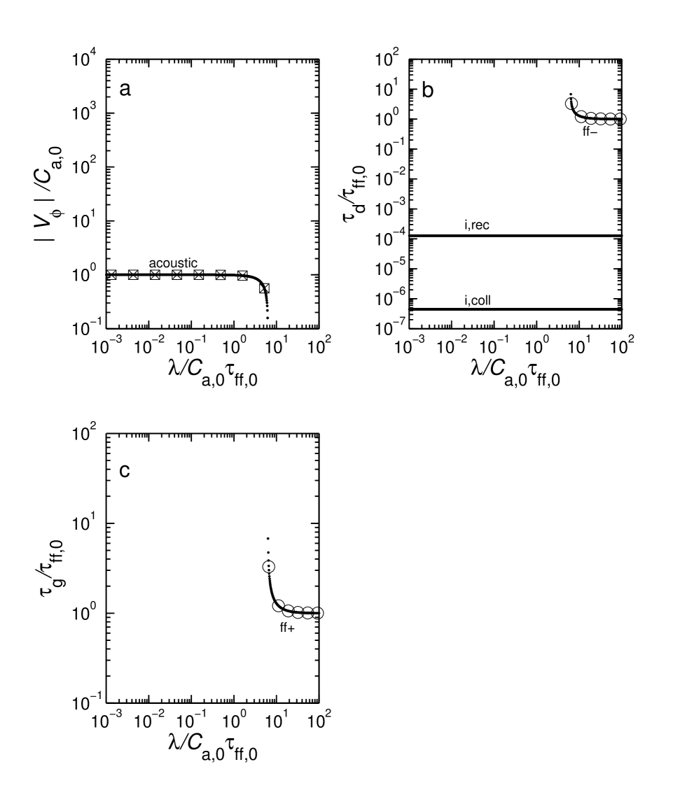
Figure 2: Eigenvalues of longitudinal modes as functions of wavelength, normalised to $C_{\rm{a},0}\tau_{{}_{\rm{ff,0}}}=9.72\times 10^{-2}~{}\rm{pc}$, at an angle of propagation $\theta=0^{\circ}$ with respect to $\mbox{\boldmath$B$}_{0}$. Because of degeneracy, there are a total of four different modes at each wavelength. Each curve is identified by a label (a mnemonic for the mode it represents) as explained in Table 1. (a) Absolute value of the phase velocity ${v}_{\phi}$, normalised to $C_{\rm{a},0}=0.243~{}\rm{km}~{}\rm{s}^{-1}$. Also overplotted as boxes with interior $\times$’s are values obtained from eq. (19). (b) Damping timescale $\tau_{{}_{\rm{d}}}$, in units of $\tau_{{}_{\rm{ff,0}}}=3.92\times 10^{5}~{}\rm{yr}$. Also shown (open circles) are values calculated from eq. (21). (c) Growth timescale $\tau_{{}_{\rm{gr}}}$, normalised to $\tau_{{}_{\rm{ff,0}}}$. Also plotted (open circles) are values calculated using eq. (21).

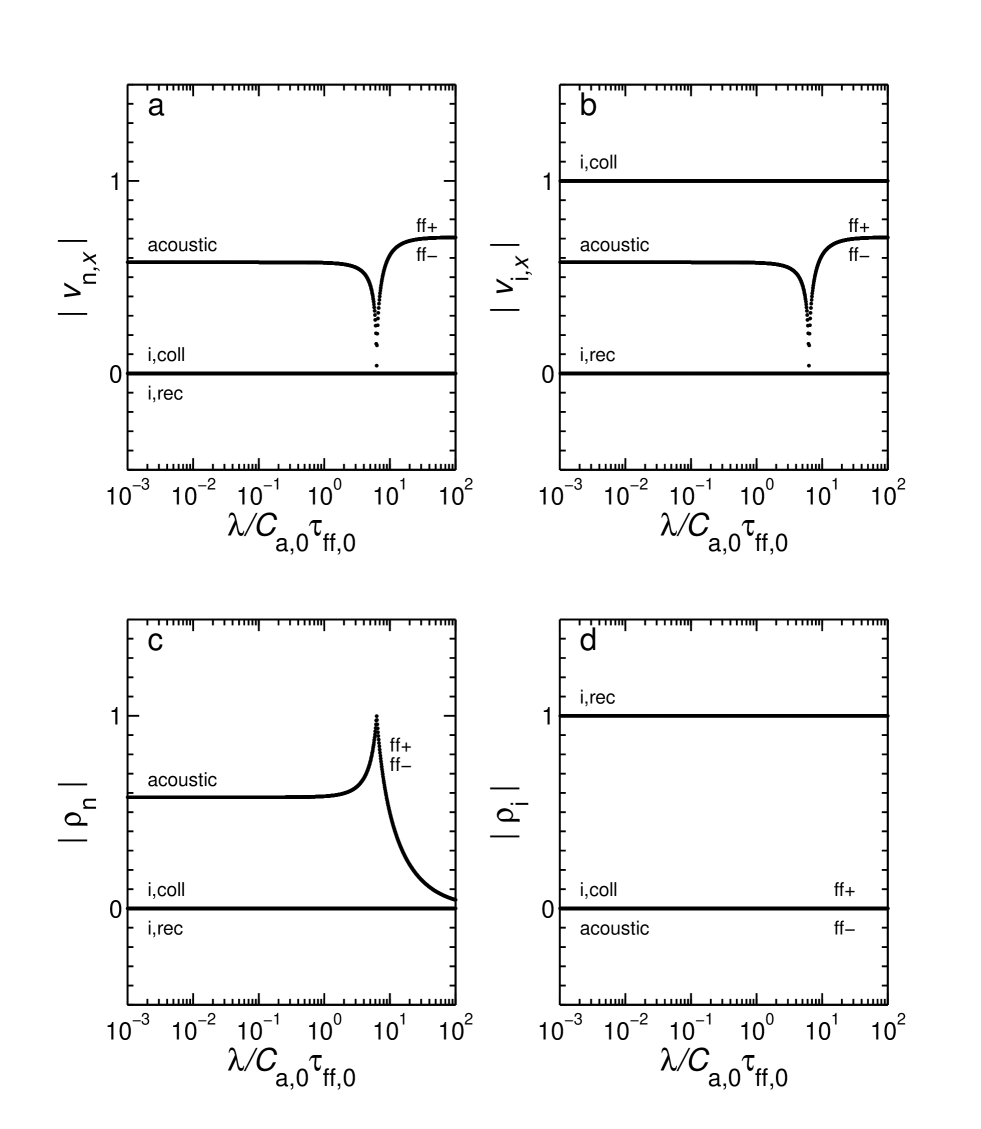
Figure 3: Magnitudes of eigenvectors of longitudinal modes for $\theta=0^{\circ}$ as functions of wavelength, normalised as in Fig. 2. As in Fig. 2, there are a total of four modes. All eigenvectors have been normalised to unity. Each curve is identified by a label (a mnemonic for the mode it represents) as explained in Table 1. (a) Longitudinal ($x$-) component of the neutral velocity, $|v_{{\rm n},x}|$. (b) Longitudinal ($x$-) component of the ion velocity, $|v_{{\rm i},x}|$. (c) Neutral density $|\rho_{\rm n}|$. (d) Ion density $|\rho_{\rm i}|$.

The first mode for this system of equations is a nonpropagating, ion collisional-decay mode, i.e., the ions are streaming through a sea of fixed neutrals. Their motion decays because of ion-neutral collisions. It is characterized by $\tilde{v}_{{\rm n},x}=0=\tilde{\rho}_{\rm n}$. Solving equations (12a) - (12d) under these conditions (or, equivalently, solving eq. [15] in the limit $|\tilde{\omega}|\gg 1/\tilde{\tau}_{{\rm{ni,0}}}$), one finds

$$\tilde{\omega}=-\frac{i}{\tilde{\tau}_{{\rm{in,0}}}}.$$ (16)

Hence, $\tilde{v}_{\phi}=0$ and $\tilde{\tau}_{{}_{\rm{d}}}=\tilde{\tau}_{{\rm{in,0}}}=4.45\times 10^{-7}$ (see Fig. 2$b$, line labeled “i,coll”). This mode is independent of wavelength (see Figs. $2b$, $3a-3d$, lines labeled “i,coll”).

The second mode is one in which density enhancements in the ions rapidly decay by dissociative recombinations of molecular ions and electrons; because the degree of ionisation is so small ($x_{\rm i,0}=1.58\times 10^{-7}$), this mode does not involve any motion of the neutrals and leaves the neutral density essentially unchanged (see Figs. $3a$ and $3c$, lines labeled “i,rec”). Solving equation (12b) with $\tilde{\rho}_{\rm n}=0$ and $\tilde{v}_{{\rm i},x}=0$, one finds that $\tilde{v}_{\phi}=0$ and

$$\tilde{\tau}_{{}_{\rm{d}}}=\left(2\tilde{\alpha}_{\rm{m,dr}}\tilde{\rho}_{\rm{i,0}}\right)^{-1}~{},$$ (17)

which is equal to $1.28\times 10^{-4}$ for the model described here. It is again the case that this mode is independent of $\tilde{k}$ (see Figs. $2b$ and $3a$ - $3d$, lines labeled “i,rec”).

The remaining two longitudinal modes are low-frequency modes, with $|\tilde{\omega}|\ll 1/\tilde{\tau}_{{\rm{in,0}}}$. Because the inertia of the ions along the magnetic field is small ($\rho_{\rm i,0}\ll\rho_{\rm n,0}$), the neutrals are able to sweep up the ions, and, as a result, $\tilde{v}_{{\rm i},x}\simeq\tilde{v}_{{\rm n},x}$ (see Figs. 3$a$ and 3$b$). For these conditions, equation (15) yields the thermal Jeans modes

$$\tilde{\omega}=\pm\tilde{k}\left[1-\left(\frac{1}{\tilde{k}^{2}}\right)\right]^{1/2}$$ (18)

(e.g., see Chandrasekhar 1961, Ch. XIII; or Spitzer 1978, § 13.3a). Therefore, for $\tilde{k}>1$,

$$\tilde{v}_{\phi}=\pm\left[1-\left(\frac{\tilde{\lambda}}{2\pi}\right)^{2}\right]^{1/2};$$ (19)

i.e., the two acoustic waves have the same phase velocity, modified by gravity, but propagate in opposite directions (along the field lines). In the limit $\tilde{\lambda}\ll 1$, $\tilde{v}_{\phi}=\pm 1$ and $\tilde{\tau}_{{}_{\rm{d}}}=\infty$; i.e., these modes are undamped sound waves (recall that the unit of speed is $C_{\rm{a},0}$). At longer wavelengths, gravitational forces become increasingly more important and the phase velocity becomes less than unity (see Fig. $2a$). The waves are gravitationally suppressed (i.e., $\tilde{v}_{\phi}=0$) at wavelengths greater than the thermal Jeans wavelength

$$\tilde{\lambda}_{\rm{J,th}}=2\pi$$ (20)

($=2\pi C_{\rm{a},0}\tau_{{}_{\rm{ff,0}}}=0.611~{}\rm{pc}$, dimensionally). For $\tilde{\lambda}>\tilde{\lambda}_{\rm{J,th}}$ (i.e, $\tilde{k}<1$), it follows from equation (18) that each of the Jeans modes splits into two separate, conjugate modes. One is a gravitational growth (or fragmentation) mode, with timescale

$$\tilde{\tau}_{{}_{\rm{gr}}}=\left[1-\left(\frac{\tilde{\lambda}_{\rm{J,th}}}{\tilde{\lambda}}\right)^{2}\right]^{-1/2}$$ (21)

(see Fig. $2c$). This is the classical Jeans instability. As $\tilde{\lambda}\rightarrow\infty$, $\tilde{\tau}_{{}_{\rm{gr}}}\rightarrow 1$; dimensionally, this is just the free-fall timescale, $\tau_{{}_{\rm{ff,0}}}$. The corresponding eigenvector is labeled as “ff+” in Figures $3a$ - $3d$. The other mode is one of exponential decay, with damping timescale $\tilde{\tau}_{{}_{\rm{d}}}$ also given by equation (21) (see eq. [18]); it is the curve labeled by “ff$-$” in Figure $2b$. The eigenvector, also labeled by “ff$-$”, is shown in Figures $3a$ - $3d$. This mode is one in which an initial density enhancement causes expansive motion, opposed by gravity, at such a rate that the density enhancement decreases to zero at the same time that the velocity vanishes. Hence, this is a monotonically decaying mode; no wave motion is involved. It is similar to the well-known classical cosmological problem of an expanding “flat” universe. Note that, as $\tilde{\lambda}\rightarrow\infty$, $\tilde{\tau}_{{}_{\rm{d}}}\rightarrow 1$.

In order to better understand the neutral thermal (Jeans) modes, we examine more closely the eigenvectors (and their features shown in Figures $3a$ - $3d$). We substitute equation (18) in equation (12a), and we use the normalisation condition $|\tilde{\rho}_{\rm n}|^{2}+|\tilde{v}_{{\rm n},x}|^{2}+|\tilde{v}_{{\rm i},x}|^{2}=1$ and the fact that $|\tilde{v}_{{\rm n},x}|=|\tilde{v}_{{\rm i},x}|$ to find that

$$|\tilde{\rho}_{\rm n}|^{2} = \frac{\tilde{k}^{2}}{3\tilde{k}^{2}-2}$$ (22a)

and

$$|\tilde{v}_{{\rm n},x}|^{2} = \frac{\tilde{k}^{2}-1}{3\tilde{k}^{2}-2}.$$ (22b)

From these equations, it follows that

• as $\tilde{k}\rightarrow\infty$ ($\tilde{\lambda}\rightarrow 0$), $|\tilde{\rho}_{\rm n}|=|\tilde{v}_{{\rm n},x}|=|\tilde{v}_{{\rm i},x}|\rightarrow 1/\sqrt{3})=0.577$, as seen in Figures $3a$ - $3c$ (curves labeled “acoustic”);

• as $\tilde{k}\rightarrow 1$ ($\tilde{\lambda}\rightarrow$ 2$\pi$), $|\tilde{\rho}_{\rm n}|\rightarrow 1$ but $|\tilde{v}_{{\rm n},x}|=|\tilde{v}_{{\rm i},x}|\rightarrow 0$, as also seen in Figures $3a$ - $3c$;

• for $\tilde{k}<\left(2/3\right)^{1/2}$ (i.e., $\tilde{\lambda}>\left(3/2\right)^{1/2}2\pi=7.70$), $~{}\tilde{\rho}_{\rm n}$ becomes imaginary (its absolute value is shown in Fig. $3c$);

• for $\left(2/3\right)^{1/2}<\tilde{k}<1$ (i.e., $2\pi<\tilde{\lambda}<7.70$), $~{}\tilde{v}_{{\rm n},x}=\tilde{v}_{{\rm i},x}$ is imaginary (Figs. $3a$ and $3b$ show the absolute values of these velocities).

For the convenience of the reader, Table 1 contains a list of all abbreviations (and their meaning) used to label the curves in all the figures of this paper.

Table 1: Glossary of Labels in Figures

Label	Meaning
acoustic	neutral acoustic wave
i,coll	ion collisional-decay mode
i,rec	ion dissociative-recombination mode
ff+	Jeans free-fall mode
ff$-$	conjugate Jeans (“cosmological”) mode
i,A	ion Alfvén wave
n,A	neutral Alfvén wave
AD	magnetically-driven ambipolar-diffusion mode
n,coll	neutral collisional-decay mode
i,ms	ion magnetosonic wave
n,ms	neutral magnetosonic wave
PD	neutral pressure-driven diffusion mode
AD,fr	neutral gravitationally-driven AD fragmentation mode
i,fast	ion fast wave
n,slow	neutral slow wave
n,fast	neutral fast wave

3.1.2 Transverse Modes for $\mbox{\boldmath$k$}\parallel\mbox{\boldmath$B$}_{0}$: Eigenfrequencies and Eigenvectors

Comparing the systems of equations for the modes with motions only in the $y$ and only in the $z$ directions, (13a) - (13c) and (14a) - (14c), we note that they are identical. Hence, for propagation along the field ($\theta=0^{\circ}$), $\tilde{\omega}(\tilde{k})$ is degenerate for these, transverse modes. Figure $4a$ displays the absolute value of their phase velocity, obtained by solving the dispersion relation

$$\tilde{\omega}^{3}+i\left(\frac{1}{\tilde{\tau}_{{\rm{ni,0}}}}+\frac{1}{\tilde{\tau}_{{\rm{in,0}}}}\right)\tilde{\omega}^{2}-\left(\tilde{v}_{\rm{A,i,0}}\tilde{k}\right)^{2}\tilde{\omega}-i\frac{\left(\tilde{v}_{\rm{A,i,0}}\tilde{k}\right)^{2}}{\tilde{\tau}_{{\rm{ni,0}}}}=0.$$ (23)

(Note that, because of the degeneracy, there are four different modes.) Damping timescales are shown in Figure $4b$ as functions of $\tilde{\lambda}$. None of the modes are unstable. The absolute values of the eigenvectors are exhibited in Figure 5: $|\tilde{v}_{{\rm n},y}|$ and $|\tilde{v}_{{\rm n},z}|$ in Figure $5a$, $|\tilde{v}_{{\rm i},y}|$ and $|\tilde{v}_{{\rm i},z}|$ in Figure $5b$, and $|\tilde{B}_{y}|$ and $|\tilde{B}_{z}|$ in Figures $5c$ and $5d$. Note that the $|\tilde{B}_{y}|$ (and $|\tilde{B}_{z}|$) axis in Figure $5d$ is logarithmic in order to show the behaviour of the modes at small wavelengths.

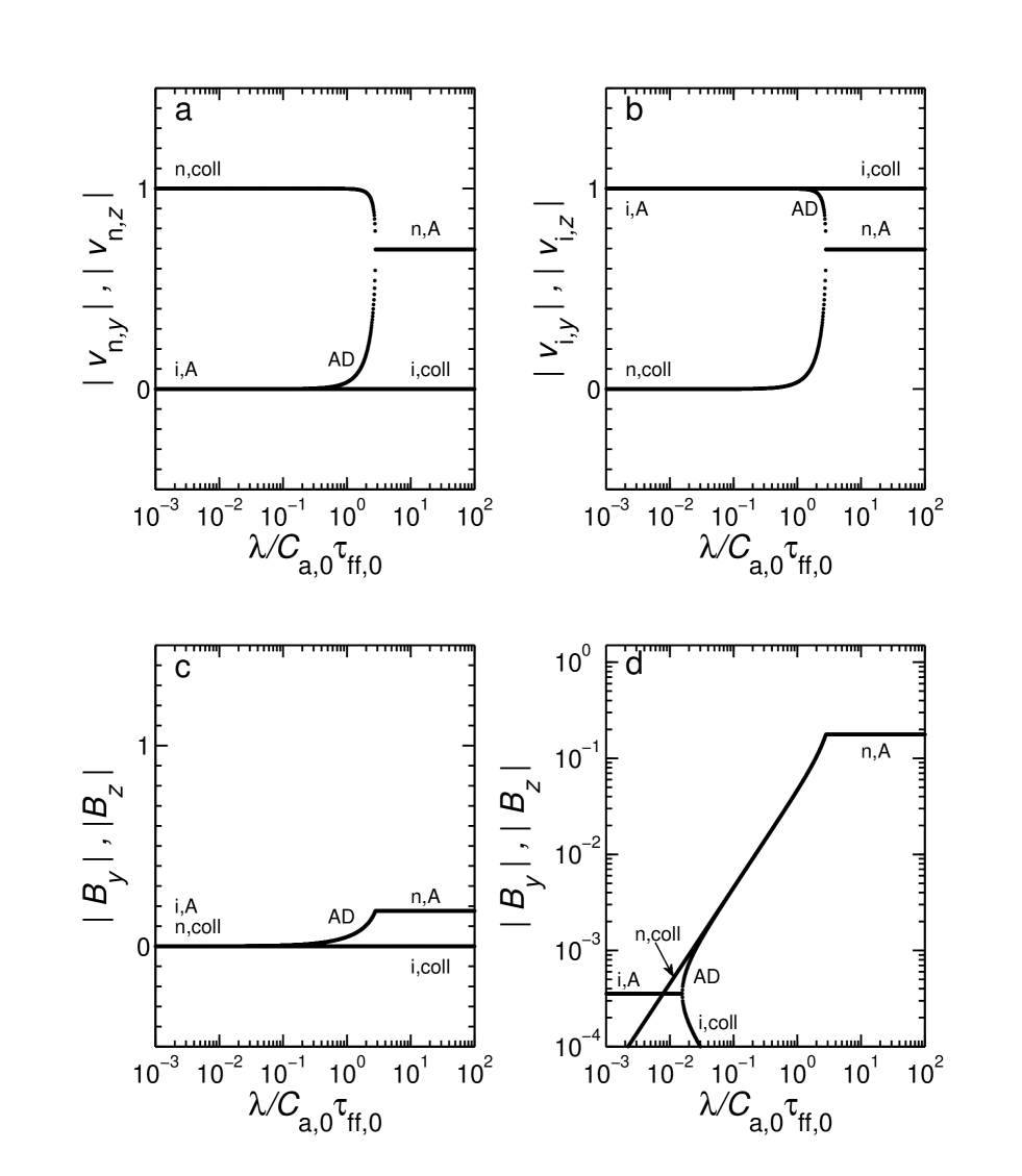
Figure 5: Magnitudes of eigenvectors of transverse modes for $\theta=0^{\circ}$ as functions of wavelength. All labels and normalisations are as in Fig. 3 and Table 1. As in Fig. 4, there are four modes at each wavelength. (a) Transverse ($y$- and $z$-) components of the neutral velocities, $|v_{{\rm n},y}|$, and $|v_{{\rm n},z}|$. (b) Transverse ($y$- and $z$-) components of the ion velocities, $|v_{{\rm i},y}|$ and $|v_{{\rm i},z}|$. (c, d) Transverse ($y$- and $z$-) components of the magnetic field, $|B_{y}|$ and $|B_{z}|$ shown on two different vertical scales, which bring out different important features (see text).

From the dispersion relation (23) and Figures $4a$ and $5a$, it is evident that small-wavelength, high-frequency ($|\tilde{\omega}|\ga 1/\tilde{\tau}_{{\rm{in,0}}}$) ion modes propagate with $\tilde{v}_{{\rm n},y}$, $\tilde{v}_{{\rm n},z}\simeq 0$. Solving equations (13a) - (13c) (or, equivalently, eqs. [14a] - [14c]) in these limits yields

$$\tilde{\omega}=\pm\tilde{v}_{\rm{A,i,0}}\tilde{k}\left[1-\left(\frac{1}{2\tilde{v}_{\rm{A,i,0}}\tilde{\tau}_{{\rm{in,0}}}\tilde{k}}\right)^{2}\right]^{1/2}-\frac{i}{2\tilde{\tau}_{{\rm{in,0}}}}.$$ (24)

(In deriving eq. [24] we have used the fact that $1/\tilde{\tau}_{{\rm{in,0}}}\gg 1/\tilde{\tau}_{{\rm{ni,0}}}$; see eqs. [11a] and [11b].) For $\tilde{\lambda}$ less than the ion Alfvén cutoff wavelength

$$\tilde{\lambda}_{\rm{A,i}}\equiv 4\pi\tilde{v}_{\rm{A,i,0}}\tilde{\tau}_{{\rm{in,0}}},$$ (25)

waves propagate with

$$\tilde{v}_{\phi}=\pm\tilde{v}_{\rm{A,i,0}}\left[1-\left(\frac{\tilde{\lambda}}{\tilde{\lambda}_{\rm{A,i}}}\right)^{2}\right]^{1/2}~{};$$ (26)

$\tilde{\lambda}_{\rm{A,i}}=1.57\times 10^{-2}$ (i.e., $\lambda_{\rm{A,i}}=1.53\times 10^{-3}~{}\rm{pc}$) for the model cloud parameters specified at the beginning of § 3. Hence, for $\tilde{\lambda}\ll\tilde{\lambda}_{\rm{A,i}}$, the waves are Alfvén waves, with $\tilde{v}_{\phi}=\pm\tilde{v}_{\rm{A,i,0}}=2.81\times 10^{3}$ (see Fig. $4a$, curve labeled “i,A”). There are four waves in all. The two polarised in the $y$-direction are normal, shear Alfvén waves, and the two polarised in the $z$-direction are modified Alfvén waves. (At $\theta>0$ the latter set of waves are fast waves.) All the waves are damped on the timescale $\tilde{\tau}_{{}_{\rm{d}}}=2\tilde{\tau}_{{\rm{in,0}}}$ (see eq. [24] and Fig. $4b$, curve labeled “i,A”) because of collisions with the neutrals. It is noteworthy that the damping time is longer by a factor of 2 than that ($\tilde{\tau}_{{\rm{in,0}}}$) referring to the dissipation (momentum exchange) of ion streaming motion relative to the neutrals. This is so because, although a typical ion indeed loses memory of the collective (wave) motion on a timescale $\tilde{\tau}_{{\rm{in,0}}}$, half of the wave energy is stored as potential energy in the magnetic field. Therefore, it takes twice as long for collisions to damp the wave than it takes them to damp ion streaming.

At $\tilde{\lambda}=\tilde{\lambda}_{\rm{A,i}}$ the ion Alfvén waves are critically damped. For $\tilde{\lambda}\geq\tilde{\lambda}_{\rm{A,i}}$, the ion-neutral collision frequency $1/\tilde{\tau}_{{\rm{in,0}}}$ is greater than the wave (angular) frequency $\tilde{\omega}$, and the waves can no longer propagate ($\tilde{v}_{\phi}=0$). At $\tilde{\lambda}=\tilde{\lambda}_{\rm{A,i}}$ there is a bifurcation in the ion modes (see Fig. $4b$). Two of the modes (one polarised in the $y$-direction and the other in the $z$-direction), corresponding to the negative root in equation (24), become ion collisional-decay modes (discussed earlier in § 3.1.1; curves labeled “i,coll” in Figs. $4b$ and $5a$ - $5d$), with

$$\tilde{\tau}_{{}_{\rm{d}}}=\frac{2\tilde{\tau}_{{\rm{in,0}}}}{1+\left[1-\left(\tilde{\lambda}_{\rm{A,i}}/\tilde{\lambda}\right)^{2}\right]^{1/2}},~{}~{}~{}~{}\tilde{\lambda}\geq\tilde{\lambda}_{\rm{A,i}}.$$ (27)

In the limit $\tilde{\lambda}\gg\tilde{\lambda}_{\rm{A,i}}$, $\tilde{B}_{y}$, $\tilde{B}_{z}\rightarrow 0$ (see Figs. $5c$ and $5d$), and $\tilde{\tau}_{{}_{\rm{d}}}\rightarrow\tilde{\tau}_{{\rm{in,0}}}$, just as in equation (16). Thus, as $\tilde{\lambda}$ increases, magnetic restoring forces on the ions become negligible, and the motion of the ions simply decays on a timescale $\tilde{\tau}_{{\rm{in,0}}}$ because of collisions with the neutrals (see Fig. $4b$, curve labeled “i,coll”). The remaining two ion modes (again, one polarised in the $y$-direction and the other in the $z$-direction), corresponding to the positive roots of the dispersion relation (eq. [24]), are magnetically-driven ambipolar-diffusion modes (see Fig. $4b$, curve labeled “AD”), in which the ions (and electrons) diffuse quasistatically (i.e., with negligible acceleration; this is equivalent to having $|\tilde{\omega}|\ll 1/\tilde{\tau}_{{\rm{in,0}}}$ in eqs. [13b] and [14b]) relative to the stationary neutrals. The damping timescale for these modes is

$$\tilde{\tau}_{{}_{\rm{d}}}=\frac{2\tilde{\tau}_{{\rm{in,0}}}}{1-\left[1-\left(\tilde{\lambda}_{\rm{A,i}}/\tilde{\lambda}\right)^{2}\right]^{1/2}},$$ (28)

which is the curve labeled as “AD” in Figure $4b$. In the limit $\tilde{\lambda}\gg\tilde{\lambda}_{\rm{A,i}}$, $\tilde{\tau}_{{}_{\rm{d}}}$ becomes equal to the ambipolar-diffusion timescale,

$$\tau_{{}_{\rm a}}=\frac{\tilde{\lambda}^{2}}{4\pi^{2}\tilde{\cal D}_{\rm{a,i}}},$$ (29a)

where

$$\tilde{\cal D}_{\rm{a,i}}\equiv\frac{\tilde{\lambda}_{\rm{A,i}}^{2}}{16\pi^{2}\tilde{\tau}_{{\rm{in,0}}}}=\tilde{v}_{\rm{A,i,0}}^{2}\tilde{\tau}_{{\rm{in,0}}}$$ (29b)

is the ion ambipolar-diffusion coefficient. For the values of the free parameters cited at the beginning of § 3, $\tilde{\cal D}_{\rm{a,i}}=3.52$.

In Figures $4b$ and $5$ it is also evident that there exists two small-wavelength, low-frequency ($|\tilde{\omega}|\ll 1/\tilde{\tau}_{{\rm{in,0}}}$) neutral modes. In these modes the plasma and magnetic field lines are essentially stationary (i.e., $\tilde{v}_{{\rm i},y}\simeq 0$, $\tilde{v}_{{\rm i},z}\simeq 0$ and $\tilde{B}_{y}\simeq 0$, $\tilde{B}_{z}\simeq 0$). Under these constraints, equations (13a) - (13c) (and, similarly, eqs. [14a] - [14c]) yield

$$\tilde{\omega}=-\frac{i}{\tilde{\tau}_{{\rm{ni,0}}}}.$$ (30)

These modes are the neutral collisional-decay modes (see curves labeled by “n,coll” in Figs. $4$ and $5$), in which the motion of the neutrals in the $y$ and $z$ directions decays due to collisions with ions that are held fixed in space by the magnetic field; $\tilde{v}_{\phi}=0$, and $\tilde{\tau}_{{}_{\rm{d}}}=\tilde{\tau}_{{\rm{ni,0}}}=0.226$ for these modes (see Fig. $4b$).

At longer wavelengths ($\sim\tilde{\lambda}_{\rm{A,n}}$, see eq. [32] below), collisions between the neutrals and the ions cause the two fluids to begin to move together. Hence, magnetic forces on the ions are more readily transmitted to the neutrals. For large enough $\tilde{\lambda}$, the neutrals can sustain a HM wave. At the point $\tilde{\lambda}=\tilde{\lambda}_{\rm{A,n}}$, the ion ambipolar-diffusion modes and the neutral collisional-decay modes merge (see Fig. $4b$); waves can propagate at longer wavelengths. In the limit $|\tilde{\omega}|\ll 1/\tilde{\tau}_{{\rm{in,0}}}$, the dispersion relation (23) has the solution

$$\tilde{\omega} = \pm\tilde{v}_{\rm{A,i,0}}\left(\frac{\tilde{\tau}_{{\rm{in,0}}}}{\tilde{\tau}_{{\rm{ni,0}}}}\right)^{1/2}\tilde{k}\left[1-\frac{\left(\tilde{v}_{\rm{A,i,0}}\tilde{\tau}_{{\rm{in,0}}}\tilde{k}\right)^{2}}{4(\tilde{\tau}_{{\rm{in,0}}}/\tilde{\tau}_{{\rm{ni,0}}})}\right]^{1/2}-\frac{i}{2}\tilde{v}_{\rm{A,i,0}}^{2}\tilde{\tau}_{{\rm{in,0}}}\tilde{k}^{2},$$ (31a)

$$= \pm\tilde{v}_{\rm{A,n,0}}\tilde{k}\left[1-\frac{1}{4}\left(\tilde{v}_{\rm{A,n,0}}\tilde{\tau}_{{\rm{ni,0}}}\tilde{k}\right)^{2}\right]^{1/2}-\frac{i}{2}\tilde{v}_{\rm{A,n,0}}^{2}\tilde{\tau}_{{\rm{ni,0}}}\tilde{k}^{2},$$ (31b)

where $\tilde{v}_{\rm{A,n,0}}$ [$=v_{\rm{A,n,0}}/C_{\rm{a},0}$, $v_{\rm{A,n,0}}\equiv B_{0}/\left(4\pi\rho_{\rm n,0}\right)^{1/2}$] is the dimensionless Alfvén speed in the neutrals. In equation (31b) we have eliminated $\tilde{\tau}_{{\rm{in,0}}}$ and $\tilde{v}_{\rm{A,i,0}}$ in favor of $\tilde{\tau}_{{\rm{ni,0}}}$ and $\tilde{v}_{\rm{A,n,0}}$ (see eqs. [3a] and [3b], and recall that $\rho_{\rm n,0}=\mu m_{\rm H}n_{\rm{n,0}}$). It follows from equation (31b) that $\tilde{v}_{\phi}>0$ for all $\tilde{\lambda}>\tilde{\lambda}_{\rm{A,n}}$, where

$$\tilde{\lambda}_{\rm{A,n}}=\pi\left(\frac{\tilde{\tau}_{{\rm{in,0}}}}{\tilde{\tau}_{{\rm{ni,0}}}}\right)^{1/2}\tilde{v}_{\rm{A,i,0}}\tilde{\tau}_{{\rm{ni,0}}}=\pi\tilde{v}_{\rm{A,n,0}}\tilde{\tau}_{{\rm{ni,0}}}$$ (32)

is the neutral Alfvén cutoff wavelength. (This is referred to simply as the Alfvén lengthscale in Mouschovias 1987a, 1991a.) In the typical model cloud, $\tilde{\lambda}_{\rm{A,n}}=2.80$, which means that the dimensional Alfvén cutoff wavelength is $\lambda_{\rm{A,n}}=0.273~{}\rm{pc}$. For $\tilde{\lambda}>\tilde{\lambda}_{\rm{A,n}}$, equations (31b) and (32) yield

$$\tilde{v}_{\phi}=\pm\tilde{v}_{\rm{A,n,0}}\left[1-\left(\frac{\tilde{\lambda}_{\rm{A,n}}}{\tilde{\lambda}}\right)^{2}\right]^{1/2}~{}.$$ (33)

In the limit $\tilde{\lambda}\gg\tilde{\lambda}_{\rm{A,n}}$, $\tilde{v}_{\phi}\rightarrow\pm\tilde{v}_{\rm{A,n,0}}$ ($=\pm 3.94$, since $|v_{\rm{A,n,0}}|=0.957~{}\rm{km}~{}\rm{s}^{-1}$); these modes are Alfvén waves in the neutrals (see curves labeled “n,A” in Figs. $4$ and $5$). The two (oppositely propagating) waves polarised in the $y$-direction are normal Alfvén waves. The two waves polarised in the $z$-direction are modified Alfvén waves; at $\theta>0$ they are fast waves. As seen from equation (31b), these modes damp on the ambipolar-diffusion timescale

$$\tilde{\tau}_{{}_{\rm{d}}}=2\tau_{{}_{\rm a}}=2\frac{\tilde{\lambda}^{2}}{4\pi^{2}\tilde{\cal D}_{\rm{a,n}}},$$ (34a)

where

$$\tilde{\cal D}_{\rm{a,n}}\equiv\frac{\tilde{\lambda}_{\rm{A,n}}^{2}}{\pi^{2}\tilde{\tau}_{{\rm{ni,0}}}}=\tilde{v}_{\rm{A,n,0}}^{2}\tilde{\tau}_{{\rm{ni,0}}}$$ (34b)

is the neutral ambipolar-diffusion coefficient. Comparing equations (29b) and (34b), we note that $\tilde{\cal D}_{\rm{a,n}}=\tilde{\cal D}_{\rm{a,i}}$ ($=3.52$ for this typical model cloud). We may therefore denote the ambipolar-diffusion coefficient simply as $\tilde{\cal D}_{\rm{a}}$, without the subscript i or n. One should bear in mind, however, that the expression for $\tilde{\tau}_{{}_{\rm{d}}}$ for the neutral Alfvén waves contains an extra factor of 2 compared to the expression for $\tilde{\tau}_{{}_{\rm{d}}}$ for the ion ambipolar-diffusion mode (compare eqs. [34a] and [29a], and make use of eqs. [34b] and [29b]). As explained in the case of the ion Alfvén waves, it takes twice as long to damp a wave than it takes to damp streaming motion (or diffusion). The existence of $\lambda_{\rm{A,n}}=\pi v_{\rm{A,n}}\tau_{\rm{ni}}$ for Alfvén waves in the neutrals was first shown by Kulsrud & Pearce (1969), who studied the excitation and propagation of HM waves in the intercloud medium due to cosmic-ray streaming (see, also, Parker 1967). Mouschovias (1987a, 1991a, b) discussed the importance of the lengthscale $\tilde{\lambda}_{\rm{A,n}}$ and the thermal Jeans lengthscale $\tilde{\lambda}_{\rm{J,th}}$ in the formation of protostellar fragments (or cores) in self-gravitating molecular clouds. He proposed that fragmentation is initiated by the decay of HM waves due to magnetically-driven ambipolar diffusion and the almost simultaneous onset of a Jeans-like instability, due to gravitationally-driven ambipolar diffusion (see discussion in § 4 below).

3.1.3 Transverse Modes for $\mbox{\boldmath$k$}\parallel\mbox{\boldmath$B$}_{0}$: Further Discussion of Eigenvectors

More insight in the physics of the transverse modes can be gained by understanding analytically certain key features of the eigenvectors shown in Figures $5a$ - $5d$. In the case of the ion Alfvén mode, we may ignore the motion of and the dissipation due to the neutrals at short wavelengths and we may use equations (13b), (13c), and the dispersion relation $\tilde{\omega}\simeq\mp\tilde{v}_{\rm{A,i,0}}\tilde{k}$ (see eq. [23]), to find that

$$\frac{\tilde{v}_{{\rm i},y}}{\tilde{B}_{y}}\simeq\mp\tilde{v}_{\rm{A,i,0}}.$$ (35)

(The $\mp$ sign on the right-hand side of eq. [35] refers to propagation in the $\pm$x-direction.) Since these modes are incompressible (i.e., $\tilde{\rho}_{\rm n}=0=\tilde{\rho}_{\rm i}$), we may use the normalisation condition

$$|\tilde{v}_{{\rm i},y}|^{2}+|\tilde{B}_{y}|^{2}=1$$ (36)

to find that

$$\tilde{v}_{{\rm i},y}\simeq\frac{\tilde{v}_{\rm{A,i,0}}}{\left(\tilde{v}_{\rm{A,i,0}}^{2}+1\right)^{1/2}}\simeq 1,$$ (37a)

and

$$\tilde{B}_{y}\simeq\mp\frac{1}{\left(\tilde{v}_{\rm{A,i,0}}^{2}+1\right)^{1/2}}\simeq\mp\frac{1}{\tilde{v}_{\rm{A,i,0}}}.$$ (37b)

Since $\tilde{v}_{\rm{A,i,0}}=2.81\times 10^{3}$, it follows from the last equation that $|\tilde{B}_{y}|\simeq 3.56\times 10^{-4}$. This is in agreement with the curve labeled “i,A” in Figure $5d$, which is the same as Figure $5c$ but with a logarithmic scale for $|\tilde{B}_{y}|$ so as to show this small but finite value of $|\tilde{B}_{y}|$ at small $\tilde{\lambda}$. Similarly, the result $\tilde{v}_{{\rm i},y}\simeq 1$ is as shown in Figure $5b$, curve labeled “i,A”.

As $\tilde{\lambda}$ increases, $|\tilde{v}_{{\rm i},y}|$ remains large and $|\tilde{v}_{{\rm n},y}|$ (and $|\tilde{B}_{y}|$) small even for $\tilde{\lambda}>\tilde{\lambda}_{\rm{A,i}}$ (see Figs. $5a$ - $5d$, curves labeled “i,A”); the ion ambipolar-diffusion mode maintains a significant $|\tilde{v}_{{\rm i},y}|$ although ion Alfvén waves do not exist for $\lambda>\tilde{\lambda}_{\rm{A,i}}$. As $\tilde{\lambda}$ increases toward the neutral Alfvén cutoff wavelength $\tilde{\lambda}_{\rm{A,n}}$ (see eq. [32]), $|\tilde{v}_{{\rm i},y}|$ decreases and $|\tilde{v}_{{\rm n},y}|$ increases because the ions begin to couple to (and induce motions in) the neutrals via collisions. At exactly $\tilde{\lambda}=\tilde{\lambda}_{\rm{A,n}}$, the two velocities become equal. For $\tilde{\lambda}>\tilde{\lambda}_{\rm{A,n}}$, Alfvén waves can be sustained by the neutrals, and the magnitudes of all three quantities $\tilde{v}_{{\rm i},y}$, $\tilde{v}_{{\rm n},y}$, and $\tilde{B}_{y}$ are significant. In the long-wavelength limit, the ions are well coupled to the neutrals ($\tilde{v}_{{\rm i},y}=\tilde{v}_{{\rm n},y}$). Using the normalisation condition

$$|\tilde{v}_{{\rm n},y}|^{2}+|\tilde{v}_{{\rm i},y}|^{2}+|\tilde{B}_{y}|^{2}=2|\tilde{v}_{{\rm n},y}|^{2}+|\tilde{B}_{y}|^{2}=1$$ (38)

and equations (13b) - (13c), we now find that

$$\frac{\tilde{v}_{{\rm n},y}}{\tilde{B}_{y}}=\mp\tilde{v}_{\rm{A,n,0}},$$ (39a)

$$\tilde{v}_{{\rm n},y}=\tilde{v}_{{\rm i},y}=\frac{\tilde{v}_{\rm{A,n,0}}}{\left(1+2\tilde{v}_{\rm{A,n,0}}^{2}\right)^{1/2}}$$ (39b)

and

$$\tilde{B}_{y}=\mp\frac{1}{\left(1+2\tilde{v}_{\rm{A,n,0}}^{2}\right)^{1/2}}.$$ (39c)

Since for our typical model cloud $\tilde{v}_{\rm{A,n,0}}$ = 3.94, it follows that $\tilde{v}_{{\rm n},y}=\tilde{v}_{{\rm i},y}=0.696$ and $\tilde{B}_{y}$ = 0.177, in agreement with Figures $5a$ - $5d$, curves labeled “n,A”.

As $\tilde{\lambda}$ increases across $\tilde{\lambda}_{\rm{A,i}}$, the ion Alfvén mode disappears (damps) and bifurcates into the (ion) ambipolar-diffusion mode and the ion collisional-decay mode, as discussed in relation to Figure $4b$; hence the placement of the labels “i,A”, “AD”, and “i,coll” on these curves in Figures $5a$ - $5d$.

It is also clear from Figures $5a$ - $5d$ that the eigenvectors for both the neutral and the ion collisional-decay modes behave exactly as expected on the basis of our discussion of these modes in relation to Figure $4b$.

3.2 Propagation Perpendicular to $\mbox{\boldmath$B$}_{0}$ ($\mbox{\boldmath$k$}\perp\mbox{\boldmath$B$}_{0}$)

For $\theta=90^{\circ}$, equations (10a) - (10k) again decouple into three independent subsystems. The subsystem involving material motions in the $x$-direction is

$$\tilde{\omega}\tilde{\rho}_{\rm n} = \tilde{k}\tilde{v}_{{\rm n},x},$$ (40a)

$$\tilde{\omega}\tilde{\rho}_{\rm i} = \tilde{\rho}_{\rm{i,0}}\tilde{k}\tilde{v}_{{\rm i},x}+i\tilde{\rho}_{\rm{i,0}}^{2}\tilde{\alpha}_{\rm{m,dr}}\tilde{\rho}_{\rm n}-i2\tilde{\rho}_{\rm{i,0}}\tilde{\alpha}_{\rm{m,dr}}\tilde{\rho}_{\rm i},$$ (40b)

$$\tilde{\omega}\tilde{v}_{{\rm n},x} = \left(\tilde{k}-\frac{1}{\tilde{k}}\right)\tilde{\rho}_{\rm n}-\frac{i}{\tilde{\tau}_{{\rm{ni,0}}}}\tilde{v}_{{\rm n},x}+\frac{i}{\tilde{\tau}_{{\rm{ni,0}}}}\tilde{v}_{{\rm i},x},$$ (40c)

$$\tilde{\omega}\tilde{v}_{{\rm i},x} = \frac{i}{\tilde{\tau}_{{\rm{in,0}}}}\tilde{v}_{{\rm n},x}-\frac{i}{\tilde{\tau}_{{\rm{in,0}}}}\tilde{v}_{{\rm i},x}+\tilde{v}_{\rm{A,i,0}}^{2}\tilde{k}\tilde{B}_{z},$$ (40d)

$$\tilde{\omega}\tilde{B}_{z} = \tilde{k}\tilde{v}_{{\rm i},x}.$$ (40e)

Motions in the $y$-direction are governed by

$$\tilde{\omega}\tilde{v}_{{\rm n},y} = -\frac{i}{\tilde{\tau}_{{\rm{ni,0}}}}\tilde{v}_{{\rm n},y}+\frac{i}{\tilde{\tau}_{{\rm{ni,0}}}}\tilde{v}_{{\rm i},y},$$ (41a)

$$\tilde{\omega}\tilde{v}_{{\rm i},y} = \frac{i}{\tilde{\tau}_{{\rm{in,0}}}}\tilde{v}_{{\rm n},y}-\frac{i}{\tilde{\tau}_{{\rm{in,0}}}}\tilde{v}_{{\rm i},y},$$ (41b)

$$\tilde{\omega}\tilde{B}_{y} = 0.$$ (41c)

Similarly, the equations for the $z$-components of the neutral and ion velocities are

$$\tilde{\omega}\tilde{v}_{{\rm n},z} = -\frac{i}{\tilde{\tau}_{{\rm{ni,0}}}}\tilde{v}_{{\rm n},z}+\frac{i}{\tilde{\tau}_{{\rm{ni,0}}}}\tilde{v}_{{\rm i},z},$$ (42a)

$$\tilde{\omega}\tilde{v}_{{\rm i},z} = \frac{i}{\tilde{\tau}_{{\rm{in,0}}}}\tilde{v}_{{\rm n},z}-\frac{i}{\tilde{\tau}_{{\rm{in,0}}}}\tilde{v}_{{\rm i},z}.$$ (42b)

3.2.1 Longitudinal Modes for $\mbox{\boldmath$k$}\perp\mbox{\boldmath$B$}_{0}$: Eigenfrequencies

The dispersion relation is easily obtained from equations (40a) - (40e):

$$\left(\tilde{\omega}+2i\tilde{\rho}_{\rm{i,0}}\tilde{\alpha}_{\rm{m,dr}}\right)\left\{\tilde{\omega}^{4}+i\left(\frac{1}{\tilde{\tau}_{{\rm{in,0}}}}+\frac{1}{\tilde{\tau}_{{\rm{ni,0}}}}\right)\tilde{\omega}^{3}-\left[\left(\tilde{v}_{\rm{A,i,0}}^{2}+1\right)\tilde{k}^{2}-1\right]\tilde{\omega}^{2}\right.$$

$$\left.\hskip 60.00009pt-i\left[\frac{1}{\tilde{\tau}_{{\rm{ni,0}}}}\tilde{v}_{\rm{A,i,0}}^{2}\tilde{k}^{2}+\frac{1}{\tilde{\tau}_{{\rm{in,0}}}}\left(\tilde{k}^{2}-1\right)\right]\tilde{\omega}+\left(\tilde{k}^{2}-1\right)\tilde{v}_{\rm{A,i,0}}^{2}\tilde{k}^{2}\right\}=0.$$ (43)

Because it is a fifth-order polynomial, there are five longitudinal modes in all. The phase velocities, damping timescales, and growth timescales for the longitudinal modes are displayed in Figures $6a$, $6b$, and $6c$, respectively; eigenvectors are shown as functions of $\tilde{\lambda}$ in Figure $7a$ - $7e$.

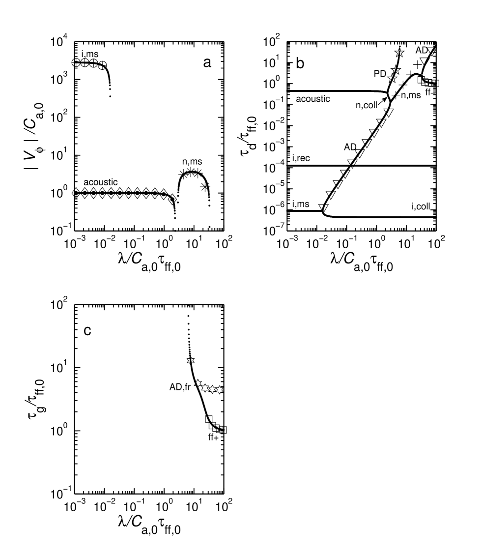
Figure 6: Eigenvalues of longitudinal modes as functions of wavelength, at an angle of propagation $\theta=90^{\circ}$ with respect to $\mbox{\boldmath$B$}_{0}$. All normalisations are as in Fig. 2. There are five different modes at each wavelength. (a) Absolute value of phase velocity, $|{v}_{\phi}|$. Phase speeds derived from eq. (26) are displayed as circles with interior crosses, while speeds obtained from eq. (45) are displayed as diamonds with interior black circles. Phase speeds determined from eq. (55) are displayed as asterisks. (b) Damping timescales $\tau_{{}_{\rm{d}}}$. Also shown are values (downward-facing triangles) calculated from eq. (29a), as well as values (plus signs) from eq. (34a). Results (five-pointed stars) from eq. (47a) are also depicted, and so are those (boxes) calculated by using eq. (56). (c) Growth timescale $\tau_{{}_{\rm{gr}}}$. Values predicted (six-pointed stars) from the ambipolar-diffusion fragmentation timescale (eq. [49]) are also displayed, along with values (boxes) calculated from the magnetic Jeans instability mode, eq. (57).

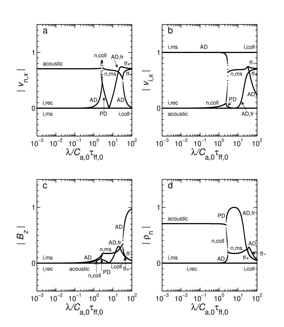
Figure 7: Magnitudes of eigenvectors of longitudinal modes for $\theta=90^{\circ}$ as functions of wavelength. All labels and normalisations are as in Fig. 3 and Table 1. As in Fig. 6, there are five modes. (a) Longitudinal ($x$-) component of the neutral velocity, $|v_{{\rm n},x}|$. (b) Longitudinal ($x$-) component of the ion velocity, $|v_{{\rm i},x}|$. (c) Magnetic field component $|B_{z}|$. (d) Neutral density $|\rho_{\rm n}|$.

Figure 7: Cont. (e) Ion density $|\rho_{\rm i}|$.

At small wavelengths there are again two high-frequency ($|\tilde{\omega}|\sim 1/\tilde{\tau}_{{\rm{in,0}}}$) ion modes, with $\tilde{v}_{{\rm n},x}\simeq 0$ (they are degenerate with respect to the direction of propagation). In this limit, the solution of the dispersion relation is identical with that given by equation (24). The modes it represents in this case are ion magnetosonic modes. Because the speed of sound of the ions ($<C_{\rm{a},0}$, since $m_{\rm{i}}>\mu m_{\rm H}$) is negligible compared to the ion Alfvén speed (see eq. [11c]), the phase velocity of the waves for $\tilde{\lambda}<\tilde{\lambda}_{\rm{A,i}}$ is again given by equation (26) and the characteristic decay time is $\tilde{\tau}_{{}_{\rm{d}}}=2\tilde{\tau}_{{\rm{in,0}}}$ (see Figs. $6a$ and $6b$, curves labeled “i,ms”). For $\tilde{\lambda}\geq\tilde{\lambda}_{\rm{A,i}}$ ($=1.57\times 10^{-2}$ for the typical model cloud) the ion magnetosonic waves cannot propagate because of frequent ion-neutral collisions. Instead, each mode bifurcates (see Fig. $6b$), just as in the case of ion Alfvén waves described in § 3.1.2. One of the two resulting modes is an ion collisional decay mode ($\tilde{\tau}_{{}_{\rm{d}}}=\tilde{\tau}_{{\rm{in,0}}}$; curve labeled “i,coll” in Fig. $6b$) and the other is a magnetically-driven ion ambipolar-diffusion mode, curve labeled “AD” in Figure $6b$ ($\tilde{\tau}_{{}_{\rm{d}}}=\tilde{\lambda}^{2}/4\pi^{2}\tilde{\cal D}_{\rm{a}}$ for $\tilde{\lambda}\gg\tilde{\lambda}_{\rm{A,i}}$; see discussion preceding eq. [29b]).

The third mode is an ion dissociative-recombination decay mode, as discussed in § 3.1.1, in which density enhancements in the ions decay rapidly [$\tilde{\tau}_{{}_{\rm{d}}}=\left(2\tilde{\rho}_{\rm{i,0}}\tilde{\alpha}_{\rm{m,dr}}\right)^{-1}=1.28\times 10^{-4}$ for the typical model cloud parameters] because of dissociative recombinations between molecular ions and electrons (see Fig. $6b$, curve labeled “i,rec”). The only nonvanishing component of the eigenvector for this mode is $\tilde{\rho}_{\rm{i,0}}$ (see Figs. $7e$ and $7a$ - $7d$).

There also exist two small-wavelength, low-frequency ($|\tilde{\omega}|\ll 1/\tilde{\tau}_{{\rm{in,0}}}$) wave modes in the neutrals. For these modes, $\tilde{v}_{{\rm i},x}\simeq 0$ and $\tilde{B}_{z}\simeq 0$ (curves labeled “acoustic” in Figs. 7b and 7c), i.e., the neutrals oscillate in the $x$-direction in an effectively fixed background of ions and magnetic field. Under these circumstances, the solution of the dispersion relation (3.2.1) is

$$\tilde{\omega}=\pm\tilde{k}\left[1-\left(1+\frac{1}{4\tilde{\tau}_{{\rm{ni,0}}}^{2}}\right)\frac{1}{\tilde{k}^{2}}\right]^{1/2}-\frac{i}{2\tilde{\tau}_{{\rm{ni,0}}}}.$$ (44)

The phase velocity can be written as

$$\tilde{v}_{\phi}=\pm\left[1-\left(\frac{\tilde{\lambda}}{\tilde{\lambda}_{\rm{s,n}}}\right)^{2}\right]^{1/2},\,\,\,\,\,{\rm for}\,\,\tilde{\lambda}<\tilde{\lambda}_{\rm{s,n}},$$ (45)

where

$$\tilde{\lambda}_{\rm{s,n}}\equiv\frac{4\pi\tilde{\tau}_{{\rm{ni,0}}}}{\left[1+(2\tilde{\tau}_{{\rm{ni,0}}})^{2}\right]^{1/2}}$$ (46)

is the acoustic-wave cutoff wavelength; $\tilde{\lambda}_{\rm{s,n}}=2.59$ in the typical model cloud. In dimensional form, $\lambda_{\rm{s,n}}\simeq 4\pi C_{\rm{a},0}\tau_{{\rm{ni,0}}}/[1+(2\tilde{\tau}_{{\rm{ni,0}}})^{2}]^{1/2}=0.252~{}\rm{pc}$. (Note that for $2\tilde{\tau}_{{\rm{ni,0}}}\ll 1$, $\tilde{\lambda}_{\rm{s,n}}\simeq 4\pi\tilde{\tau}_{{\rm{ni,0}}}$; in this limit $\lambda_{\rm{s,n}}=4\pi C_{\rm{a},0}\tau_{{\rm{ni,0}}}=0.277$ pc.) These are sound waves in the neutrals modified by gravity and neutral-ion collisions. For $\tilde{\lambda}\ll\tilde{\lambda}_{\rm{s,n}}$, $\tilde{v}_{\phi}=\pm 1$ ($=\pm C_{\rm{a},0}$, dimensionally), hence, the waves are pure sound waves (see Fig. $6a$, curve labeled “acoustic”). They decay on a timescale $\tilde{\tau}_{{}_{\rm{d}}}=2\tilde{\tau}_{{\rm{ni,0}}}$ (= 0.452; see curve labeled “acoustic” in Fig. $6b$). For $\tilde{\lambda}\geq\tilde{\lambda}_{\rm{s,n}}$, the waves are damped because of collisions with the ions, and $\tilde{v}_{\phi}=0$, much like the damping of the ion Alfvén and magnetosonic modes for $\tilde{\lambda}\geq\tilde{\lambda}_{\rm{A,i}}$. For $\tilde{\lambda}>\tilde{\lambda}_{\rm{s,n}}$, this modified neutral sound wave bifurcates (see Fig. $6b$) into a pressure-driven diffusion mode (curve labeled “PD”) and a collisional-decay mode (curve labeled “n,coll”). We examine these modes in that order.

The pressure-driven diffusion mode corresponds to the positive root of equation (44). The neutrals are diffusing quasistatically (i.e., with $|\tilde{\omega}|\ll 1/\tilde{\tau}_{{\rm{ni,0}}}$) through a background of effectively stationary ions and magnetic field. The eigenvector for this mode is labeled “PD” in Figs. $7a$ - $7e$. For $\tilde{\lambda}_{\rm{s,n}}\leq\tilde{\lambda}\leq\tilde{\lambda}_{\rm{J,th}}$, the damping timescale is

$$\tilde{\tau}_{{}_{\rm{d}}} = \frac{2\tilde{\tau}_{{\rm{ni,0}}}}{1-\left\{1-4\tilde{\tau}_{{\rm{ni,0}}}^{2}\left[\left(\tilde{\lambda}_{\rm{J,th}}/\tilde{\lambda}\right)^{2}-1\right]\right\}^{1/2}},$$ (47a)

$$\simeq \frac{(\tilde{\lambda}/\tilde{\lambda}_{\rm{J,th}})^{2}}{\tilde{\cal D}_{\rm{P}}\left[1-\left(\tilde{\lambda}/\tilde{\lambda}_{\rm{J,th}}\right)^{2}\right]},$$ (47b)

where

$$\tilde{\cal D}_{\rm{P}}\equiv\tilde{\tau}_{{\rm{ni,0}}}$$ (48)

($=C_{\rm{a},0}^{2}\tau_{{\rm{ni,0}}}$ dimensionally) is the neutral pressure-driven diffusion coefficient. In obtaining equation (47b) we have used the fact that $\tilde{\tau}_{{\rm{ni,0}}}^{2}\ll 1$. For the representative model cloud used in this paper, $\tilde{\cal D}_{\rm{P}}=0.226$ ($\simeq\tilde{\cal D}_{\rm{a}}/16$). We note that, at $\tilde{\lambda}=\tilde{\lambda}_{\rm{J,th}}$, $\tilde{\tau}_{{}_{\rm{d}}}=\infty$ (see Fig. 6$b$, curve labeled “PD”). At this wavelength, the restoring pressure forces in this mode are exactly balanced by self-gravitational forces, and the system is on the verge of gravitational instability ($\tilde{\omega}=0$). Thus the Jeans instability manifests itself at $\tilde{\lambda}_{\rm{J,th}}$ even in the presence of a magnetic field, as originally recognized by Langer (1979). Ambipolar diffusion allows this to happen, but, because of neutral-ion collisions, the growth time of the instability is longer than that of the nonmagnetic Jeans instability (compare eq. [49] below with eq. [21]). For $\tilde{\lambda}>\tilde{\lambda}_{\rm{J,th}}$, density perturbations in the neutrals grow exponentially in time as a result of gravitational contraction of neutrals through essentially stationary ions attached to rigid magnetic field lines. The growth time for this instability can be obtained easily from equation (44) under the conditions $\tilde{\lambda}>\tilde{\lambda}_{\rm{J,th}}$ and $4\tilde{\tau}_{{\rm{ni,0}}}^{2}\left[1-\left(\tilde{\lambda}_{\rm{J,th}}/\tilde{\lambda}\right)^{2}\right]\,\ll\,1$:

$$\tilde{\tau}_{{}_{\rm{gr}}}=\frac{(1/\tilde{\tau}_{{\rm{ni,0}}})}{1-\left(\tilde{\lambda}_{\rm{J,th}}/\tilde{\lambda}\right)^{2}}=\frac{\nu_{\rm{ff},0}}{1-\left(\tilde{\lambda}_{\rm{J,th}}/\tilde{\lambda}\right)^{2}},$$ (49)

where $\nu_{\rm{ff},0}=1/\tilde{\tau}_{{\rm{ni,0}}}$ ($=\tau_{{}_{\rm{ff,0}}}/\tau_{{\rm{ni,0}}}$ = 1/0.226 = 4.42) is the collapse retardation factor, discussed in the penultimate paragraph of § 2.3. It follows from equation (49) that, in the limit $\tilde{\lambda}\gg\tilde{\lambda}_{\rm{J,th}}$, $\tilde{\tau}_{{}_{\rm{gr}}}\rightarrow\nu_{\rm{ff},0}$. The growth time of this ambipolar-diffusion–induced fragmentation is shown in Figure $6c$ (the part of the curve labeled by “AD,fr”). Dimensionally, the growth time for this mode is $\nu_{\rm{ff},0}\tau_{{}_{\rm{ff,0}}}=\tau_{{}_{\rm{ff,0}}}^{2}/\tau_{{\rm{ni,0}}}$. It is the same as the nonlinear solution found analytically by Mouschovias (1979; see also 1983, 1987a, b, 1989) for the timescale of formation and evolution of protostellar cores (due to gravitationally-driven ambipolar diffusion). Numerical simulations (including the effects of grains, UV ionisation, and magnetic braking) of the formation of protostellar cores in magnetically supported molecular clouds have also found that the evolution occurs on this timescale (Fiedler & Mouschovias 1993; Ciolek & Mouschovias 1994, 1995; Basu & Mouschovias 1994, 1995a, b). The same timescale was found in the one-dimensional similarity solution of Scott (1984). It is clear from Figure $6c$ that, as predicted, $\tilde{\tau}_{{}_{\rm{gr}}}$ would tend to $1/\tilde{\tau}_{{\rm{ni,0}}}=4.42$ for $\tilde{\lambda}\gg\tilde{\lambda}_{\rm{J,th}}$; see the inflection point in the curve (labeled “AD,fr”). However, $\tilde{\tau}_{{}_{\rm{gr}}}$ falls below this would-be asymptotic value because, for $\tilde{\lambda}\ga\tilde{\lambda}_{\rm{J,mag}}$, where $\tilde{\lambda}_{\rm{J,mag}}$ is the magnetic Jeans wavelength (= 25.6; see eq. [54] below), gravitational forces on the neutrals, transmitted to the ions by neutral-ion collisions, exceed the restoring magnetic forces on the ions, and the ions and magnetic field are no longer able to remain stationary; the mode becomes a gravitational (Jeans) instability against the magnetic field, as originally found by Chandrasekhar & Fermi (1953); see Figure $6c$, part of curve beyond the inflecton point, labeled “ff+”. The approximations $\tilde{v}_{{\rm i},x}\simeq 0$, $\tilde{B}_{z}\simeq 0$ (which were used in deriving eq. [44]) are no longer valid, and equation (49) no longer describes this mode. The proper expressions are derived below.

The second mode resulting from the bifurcation of the modified sound waves at $\tilde{\lambda}_{\rm{s,n}}$ is described by the negative root of equation (44). This is a neutral collisional-decay mode (curve labeled “n,coll” in Fig. $6b$), with damping time

$$\tilde{\tau}_{{}_{\rm{d}}} = \frac{2\tilde{\tau}_{{\rm{ni,0}}}}{1+\left\{1-4\tilde{\tau}_{{\rm{ni,0}}}^{2}\left[\left(\tilde{\lambda}_{\rm{J,th}}/\tilde{\lambda}\right)^{2}-1\right]\right\}^{1/2}}$$ (50a)

$$\simeq \frac{\tilde{\tau}_{{\rm{ni,0}}}}{1-\tilde{\tau}_{{\rm{ni,0}}}^{2}\left[\left(\tilde{\lambda}_{\rm{J,th}}/\tilde{\lambda}\right)^{2}-1\right]}.$$ (50b)

In equation (50b) we have again used the fact that, for the typical model cloud, $\tilde{\tau}_{{\rm{ni,0}}}^{2}\ll 1$.

For $\tilde{\lambda}\gg\tilde{\lambda}_{\rm{J,th}}$, $\tilde{\tau}_{{}_{\rm{d}}}\rightarrow\tilde{\tau}_{{\rm{ni,0}}}$. This limit is never attained by this mode, however, because the collisional coupling between the neutrals and the ions becomes more effective with increasing $\tilde{\lambda}$, and the ions (and, hence, the magnetic field lines) begin to move with the neutrals. As a result, the neutral collisional-decay mode and the (ion) ambipolar-diffusion mode combine and merge to form wave modes, in a way similar to that for the neutral Alfvén waves in § 3.1.2 (compare Figs. $4b$ and $6b$). This mode coupling occurs at $\tilde{\lambda}=2.72$ (= $\tilde{\lambda}_{\rm{ms,n}}$; see below), which is only slightly greater than the neutral acoustic-wave cutoff $\tilde{\lambda}_{\rm{s,n}}=2.59$ for the typical model cloud (see Fig. $6b$). The solution of the dispersion relation (eq. [3.2.1]) for these modes in the limit $|\tilde{\omega}|\ll 1/\tilde{\tau}_{{\rm{in,0}}}$ is

$$\tilde{\omega}=\pm\tilde{v}_{\rm{ms,n,0}}\tilde{k}\left[1-\frac{1}{\tilde{v}_{\rm{ms,n,0}}^{2}\tilde{k}^{2}}-\frac{\left(\tilde{v}_{\rm{A,n,0}}^{2}\tilde{\tau}_{{\rm{ni,0}}}\tilde{k}\right)^{2}}{16\tilde{v}_{\rm{ms,n,0}}^{2}}\right]^{1/2}-\frac{i}{4}\tilde{v}_{\rm{A,n,0}}^{2}\tilde{\tau}_{{\rm{ni,0}}}\tilde{k}^{2},$$ (51)

where

$$\tilde{v}_{\rm{ms,n,0}}=\left(\tilde{v}_{\rm{A,n,0}}^{2}+1\right)^{1/2}$$ (52)

[or, in dimensional form, $v_{\rm{ms,n,0}}=\{v_{\rm{A,n,0}}^{2}+C_{\rm{a},0}^{2}\}^{1/2}$] is the magnetosonic speed in the neutrals. For the representative model cloud used in this paper, $\tilde{v}_{\rm{ms,n,0}}=4.07=1.03\tilde{v}_{\rm{A,n,0}}$. Examination of equation (51) reveals that $\tilde{\omega}_{\rm r}>0$ (i.e., $\tilde{v}_{\phi}>0$) if $\tilde{\lambda}_{\rm{ms,n}}<\tilde{\lambda}<\tilde{\lambda}_{\rm{J,mag}}$, where

$$\tilde{\lambda}_{\rm{ms,n}}=\frac{\pi\tilde{v}_{\rm{A,n,0}}^{2}\tilde{\tau}_{{\rm{ni,0}}}}{\tilde{v}_{\rm{ms,n,0}}}=\left(\frac{\tilde{v}_{\rm{A,n,0}}}{\tilde{v}_{\rm{ms,n,0}}}\right)\tilde{\lambda}_{\rm{A,n}}$$ (53)

is the neutral magnetosonic cutoff wavelength, and

$$\tilde{\lambda}_{\rm{J,mag}}=2\pi\tilde{v}_{\rm{ms,n,0}}$$ (54)

(or, in dimensional form, $\lambda_{\rm{J,mag}}=2\pi v_{\rm{ms,n,0}}\tau_{{}_{\rm{ff,0}}}$) is the magnetic Jeans wavelength. For the typical model cloud, $\tilde{\lambda}_{\rm{ms,n}}=2.72$ and $\tilde{\lambda}_{\rm{J,mag}}=25.6$ (hence, $\lambda_{\rm{ms,n}}=0.264~{}\rm{pc}$, and $\lambda_{\rm{J,mag}}=2.49~{}\rm{pc}$). [Note: in deriving equations (53) and (54), we have used the fact that, for the conditions of interest, $\tilde{\tau}_{{\rm{ni,0}}}^{2}\ll 1$ and $1/\tilde{v}_{\rm{ms,n,0}}^{2}\ll 1$.] Inserting equations (53) and (54) in equation (51), the phase velocity for magnetosonic waves in the neutrals is found to be

$$\tilde{v}_{\phi}=\pm\tilde{v}_{\rm{ms,n,0}}\left[1-\left(\frac{\tilde{\lambda}}{\tilde{\lambda}_{\rm{J,mag}}}\right)^{2}-\left(\frac{\tilde{\lambda}_{\rm{ms,n}}}{\tilde{\lambda}}\right)^{2}\right]^{1/2},~{}~{}~{}~{}\tilde{\lambda}_{\rm{ms,n}}\leq\tilde{\lambda}\leq\tilde{\lambda}_{\rm{J,mag}}$$ (55)

(see Fig. $6a$, curve labeled “n,ms”). The waves are weakly damped by ambipolar diffusion (see Fig. $6b$, curve labeled “n,ms”); $\tilde{\tau}_{{}_{\rm{d}}}=2\tilde{\lambda}^{2}/4\pi^{2}\tilde{\cal D}_{\rm{a}}$ (see eqs. [34b] and [51]).

For $\tilde{\lambda}\ga\tilde{\lambda}_{\rm{J,mag}}$, gravitational forces on the neutrals overwhelm the restoring magnetic forces, and the neutral magnetosonic modes become gravitationally suppressed ($\tilde{v}_{\phi}=0$), just like the thermal Jeans modes become suppressed for $\tilde{\lambda}\geq\tilde{\lambda}_{\rm{J,th}}$ (see discussion in § 3.1.1). For $\tilde{\lambda}\simeq\tilde{\lambda}_{\rm{J,mag}}$, each (neutral) magnetosonic mode bifurcates into an ambipolar-diffusion mode (with damping timescale $\tilde{\tau}_{{}_{\rm{d}}}=\tilde{\lambda}^{2}/4\pi^{2}\tilde{\cal D}_{\rm{a}}$ for $\tilde{\lambda}\gg\tilde{\lambda}_{\rm{J,mag}}$) and a conjugate Jeans mode (with damping timescale $\tilde{\tau}_{{}_{\rm{d}}}=1$ for $\tilde{\lambda}\gg\tilde{\lambda}_{\rm{J,mag}}$); see Figure $6b$, curves labeled “AD” and “ff$-$”, respectively.

The conjugate Jeans (or classical cosmological) mode was discussed earlier in connection with equation (18). In this mode the neutrals, ions, and magnetic field lines are well coupled, but the gravitational forces prevent them from oscillating; motions are damped monotonically. The damping time, corresponding to the negative root of equation (51), for $\tilde{\lambda}\geq\tilde{\lambda}_{\rm{J,mag}}$ is given by

$$\tilde{\tau}_{{}_{\rm{d}}}=\left\{\left[1-\left(\frac{\tilde{\lambda}_{\rm{J,mag}}}{\tilde{\lambda}}\right)^{2}+\left(\frac{2\pi^{2}\tilde{\cal D}_{\rm{a}}}{\tilde{\lambda}^{2}}\right)^{2}\right]^{1/2}+\frac{2\pi^{2}\tilde{\cal D}_{\rm{a}}}{\tilde{\lambda}^{2}}\right\}^{-1}.$$ (56)

It is clear that, in the limit $\tilde{\lambda}\rightarrow\infty$, $\tilde{\tau}_{{}_{\rm{d}}}\rightarrow 1$ (i.e., $\tau_{\rm d}=\tau_{{}_{\rm{ff,0}}}$); see Figure $6b$, curve labeled “ff$-$”.

Finally, the gravitational instability mode (see eq. [49]) also changes behaviour at $\tilde{\lambda}_{\rm{J,mag}}$, as discussed above. For $\tilde{\lambda}>\tilde{\lambda}_{\rm{J,mag}}$, the neutrals, plasma, and magnetic field lines are well coupled and behave like a single fluid; self-gravity overwhelms restoring magnetic and thermal-pressure forces, and the mode behaves as a classical Jeans instability, in which density perturbations grow exponentially in time with a timescale

$$\tilde{\tau}_{{}_{\rm{gr}}}=\left\{\left[1-\left(\frac{\tilde{\lambda}_{\rm{J,mag}}}{\tilde{\lambda}}\right)^{2}+\left(\frac{2\pi^{2}\tilde{\cal D}_{\rm{a}}}{\tilde{\lambda}^{2}}\right)^{2}\right]^{1/2}+\frac{2\pi^{2}\tilde{\cal D}_{\rm{a}}}{\tilde{\lambda}^{2}}\right\}^{-1},$$ (57)

which is equal to the damping time of the conjugate Jeans mode (see eq. [56]). From this equation we see that $\tilde{\tau}_{{}_{\rm{gr}}}\rightarrow 1$ (i.e., $\tau_{\rm{gr}}=\tau_{{}_{\rm{ff,0}}}$) for $\tilde{\lambda}\rightarrow\infty$, in agreement with the long-wavelength behaviour of $\tilde{\tau}_{{}_{\rm{gr}}}$ exhibited in Figure $6c$.

3.2.2 Longitudinal Modes for $\mbox{\boldmath$k$}\perp\mbox{\boldmath$B$}_{0}$: Eigenvectors

The main features of the eigenvectors are as follows.

• The dominant component of the ion magnetosonic and the ion ambipolar-diffusion modes is $\tilde{v}_{{\rm i},x}$ (see Fig. $7b$, curves labeled “i,ms” and “AD”). It does not vanish at $\tilde{\lambda}=\tilde{\lambda}_{\rm{A,i}}$; in fact, it hardly changes from 1, because the ion-AD mode maintains $\tilde{v}_{{\rm i},x}$ large beyond $\tilde{\lambda}_{\rm{A,i}}$. Only when the ion-AD mode induces motions in the neutrals does $\tilde{v}_{{\rm i},x}$ begin to decrease, as the magnitude of $\tilde{v}_{{\rm n},x}$ increases as $\tilde{\lambda}\rightarrow\tilde{\lambda}_{\rm{ms,n}}$ (see Figs. $7b$ and $7a$, curves labeled “i,ms” and “AD”). The $z$-component of the magnetic field $\tilde{B}_{z}$ in Figure $7c$ actually does not vanish. It is equal to $\tilde{v}_{{\rm i},x}/\tilde{v}_{\rm i,ms}$ (see eq. [35]), but $\tilde{v}_{\rm i,ms}\simeq v_{\rm{A,i,0}}=2.81\times 10^{3}$.
  

• The velocity $\tilde{v}_{{\rm i},x}$ is also the dominant component of the eigenvector of the ion collisional-decay mode at all wavelengths (see Fig. $7b$, curve labeled “i,coll”).
  

• The eigenvector of the neutral acoustic mode has significant components $\tilde{v}_{{\rm n},x}$ and $\tilde{\rho}_{\rm n}$. At $\tilde{\lambda}_{\rm{s,n}}$, beyond which neutral sound waves do not exist and at which the acoustic mode bifurcates into the neutral collisional-decay mode and the pressure-diffusion mode (see Fig. $6b$), the collisional-decay mode is responsible for the increase in $|\tilde{v}_{{\rm n},x}|$ as $|\tilde{\rho}_{\rm n}|$ decreases to zero. Because motion is induced in the ions as $\tilde{\lambda}$ approaches $\tilde{\lambda}_{\rm{s,n}}$ (see Fig. $7b$, curve labeled “n,coll”), $|\tilde{v}_{{\rm n},x}|$ does not reach unity.
  

• The most significant component of the PD mode is $\tilde{\rho}_{\rm n}$ (see Fig. $7d$); $\tilde{\rho}_{\rm n}$ increases as $\tilde{\lambda}$ increases from $\tilde{\lambda}_{\rm{s,n}}$ to $\tilde{\lambda}_{\rm{J,th}}$, at which wavelength $\tilde{\rho}_{\rm n}$ reaches a maximum. Beyond $\tilde{\lambda}_{\rm{J,th}}$, ambipolar-diffusion–induced fragmentation sets in. At exactly $\tilde{\lambda}_{\rm{J,th}}$, $\tilde{\rho}_{\rm n}$ is the only nonvanishing component of the eigenvector of the AD,fr mode (see Figs. $7a$ - $7d$). As $\tilde{\lambda}$ increases beyond $\tilde{\lambda}_{\rm{J,th}}$, the field lines begin to be compressed as the neutrals begin to couple to the ions, and $\tilde{B}_{z}$ increases (see Fig. $7c$) – at the expense of $\tilde{\rho}_{\rm n}$ – while $\tilde{v}_{{\rm i},x}$ and $\tilde{v}_{{\rm n},x}$ are negligible. As $\tilde{\lambda}$ approaches $\tilde{\lambda}_{\rm{J,mag}}$, the ambipolar-diffusion–fragmentation mode induces significant velocities $\tilde{v}_{{\rm n},x}$ and $\tilde{v}_{{\rm i},x}$, while $\tilde{\rho}_{\rm n}$ remains large (see Figs. $7a$, $7b$ and $7d$). As discussed in relation to Figure $6c$, the AD,fr mode turns into the Jeans free-fall mode (ff+) beyond $\tilde{\lambda}\simeq\tilde{\lambda}_{\rm{J,mag}}$, as is clearly shown in Figures $7a$ and $7b$ (see curves labeled “AD,fr” and “ff+”). The bifurcation of the neutral magnetosonic mode into the AD and conjugate Jeans (or, cosmological, ff-) modes beyond $\tilde{\lambda}\simeq\tilde{\lambda}_{\rm{J,mag}}$, discussed in relation to Figure $6b$, is also seen clearly in Figures $7a$ and $7b$. [Note: If we had plotted only the real part of the eigenvector, we would have found, for the neutral magnetosonic mode, that $\rm{Re}\{\tilde{\rho}_{\rm n}\}$ decreases discontinuously to zero, then increases smoothly, reaches a maximum, and then vanishes again as the magnetosonic waves are suppressed by gravity.]
  

• Slightly beyond $\tilde{\lambda}_{\rm{ms,n}}$, magnetosonic waves exist in the neutrals but, in addition to maintaining $\tilde{v}_{{\rm n},x}$ large, they cause significant motion in the ions as well (see Figs. $7a$ and $7b$, curves labeled “n,ms”). The quantities $\tilde{B}_{z}$ and $\tilde{\rho}_{\rm n}$ are also nonnegligible. Note that at $\tilde{\lambda}_{\rm{J,th}}$, $\tilde{v}_{{\rm n},x}$ and $\tilde{\rho}_{\rm n}$ decrease while $\tilde{v}_{{\rm i},x}$ increases.

3.2.3 Transverse Modes for $\mbox{\boldmath$k$}\perp\mbox{\boldmath$B$}_{0}$

Examination of equation (41c) reveals that there is one trivial mode with $\tilde{\omega}=0$. The remaining equations governing the transverse modes with motions in the $y$-direction (eqs. [41a] and [41b]) are identical with those in the $z$-direction (eqs. [42a] and [42b]). Solving this simple system, we find that

$$\tilde{\omega}=0,$$ (58a)

and

$$\tilde{\omega}=-i\left(\frac{1}{\tilde{\tau}_{{\rm{in,0}}}}+\frac{1}{\tilde{\tau}_{{\rm{ni,0}}}}\right)\simeq-\frac{i}{\tilde{\tau}_{{\rm{in,0}}}},$$ (58b)

both of which are independent of wavelength. (Note: there are four modes in all, two corresponding to the first solution, and two corresponding to the second.) In the first mode the ions and neutrals move together with $\tilde{v}_{{\rm n},y}=\tilde{v}_{{\rm i},y}$ (or $\tilde{v}_{{\rm n},z}=\tilde{v}_{{\rm i},z}$); hence, there are no frictional forces between the two species, and $\tilde{\tau}_{{}_{\rm{d}}}=\infty$. The second mode consists of oppositely flowing streams of ions and neutrals. The momentum of each species decays by collisions with the other; hence, ion-neutral and neutral-ion collisions occur in parallel, and the net damping time for this mode is the harmonic mean of $\tilde{\tau}_{{\rm{in,0}}}$ and $\tilde{\tau}_{{\rm{ni,0}}}$ (see eq. [58b]). For the typical model cloud, the ion fluid has a much smaller inertia than the neutral fluid and, therefore, the streaming velocity of the ions is much greater than that of the neutrals. As a result, the motion of the ions is collisionally damped on the timescale $\tilde{\tau}_{{}_{\rm{d}}}\simeq\tilde{\tau}_{{\rm{in,0}}}$.

3.3 Propagation at Angles $0^{\circ}\,<\,\theta\,<\,90^{\circ}$ with respect to $\mbox{\boldmath$B$}_{0}$

Equations (10a) - (10k) reveal that, for $0^{\circ}\leq\theta\leq 90^{\circ}$, the equations for the modes with motions in the $y$-direction are uncoupled from those with motions in the $(x,z)$-plane. Motions in the $x$- and $z$-direction, however, are coupled. The modes with $\tilde{v}_{{\rm n},y}\neq 0\neq\tilde{v}_{{\rm i},y}$ (governed by eqs. [10f] - [10h]) are purely transverse; those with nonvanishing velocities in the $(x,z)$-plane (governed by eqs. [10a] - [10e] and [10i] - [10k]) are neither purely longitudinal nor purely transverse.

3.3.1 Transverse Modes

Figures $8a$ and $8b$ display the magnitude of the phase velocities and the damping timescales of the three transverse modes for propagation at an angle $\theta=45^{\circ}$ with respect to $\mbox{\boldmath$B$}_{0}$. Because they are incompressible, none of these modes can become gravitationally unstable. Eigenvectors are displayed in Figure 9.

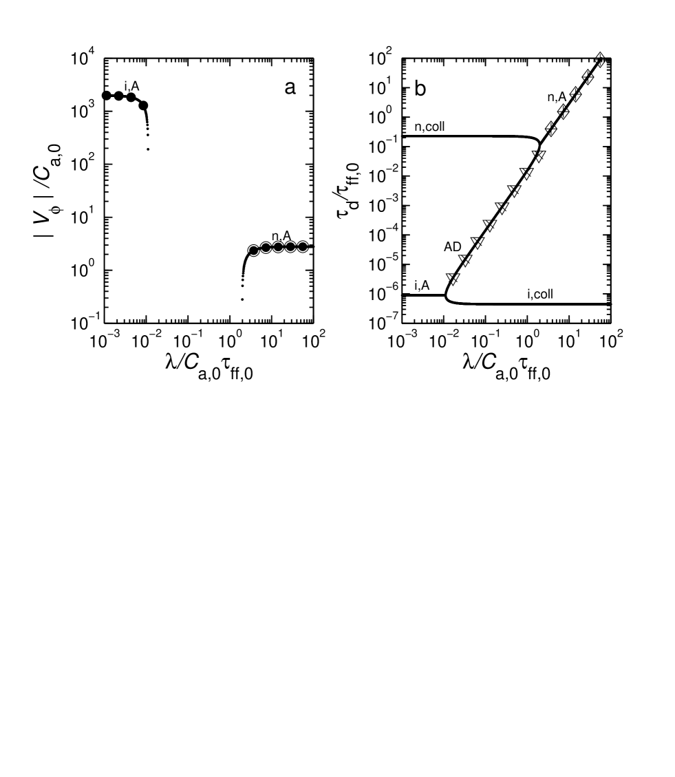
Figure 8: Eigenvalues of transverse modes as functions of wavelength, at an angle of propagation $\theta=45^{\circ}$ with respect to $\mbox{\boldmath$B$}_{0}$. All normalisations and labels are as in Fig. 2 and Table 1. There are three different modes. (a) Absolute value of phase velocity, $|{v}_{\phi}|$. Phase speeds (large black circles) obtained from eq. (59) are shown, in addition to those calculated from eq. (61) (open circles with interior black circles). (b) Damping timescales $\tau_{{}_{\rm{d}}}$. Also depicted are values (downward-facing triangles with $\times$’s inside) obtained from eq. (60), and values (diamonds with interior crosses) obtained from eq. (62).

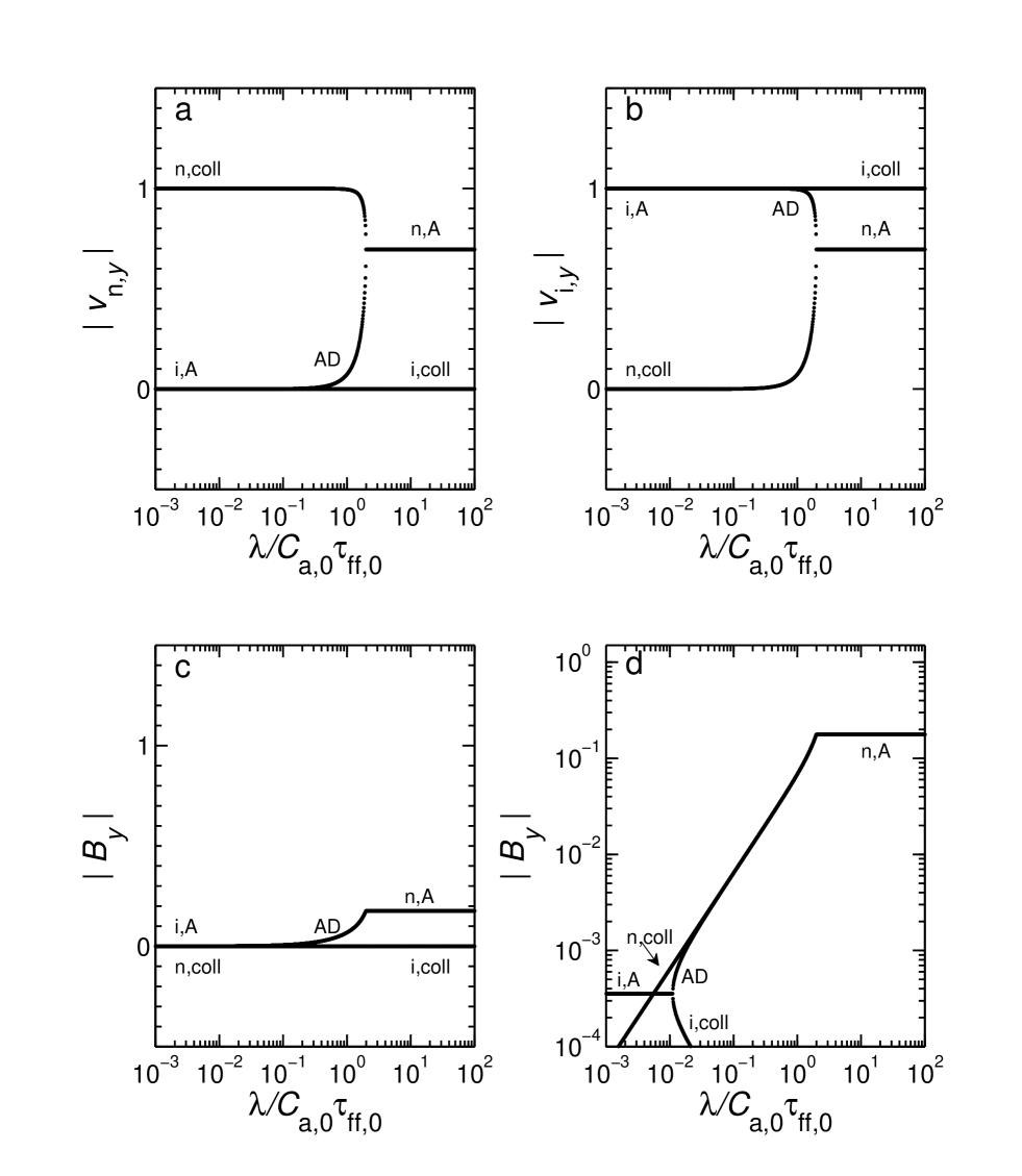
Figure 9: Magnitudes of eigenvectors of transverse modes for $\theta=45^{\circ}$ as functions of wavelength. All labels and normalisations are as in Fig. 3 and Table 1. As in Fig. 8, there are three modes. (a) Transverse ($y$-) component of the neutral velocity, $|v_{{\rm n},y}|$. (b) Transverse ($y$-) component of the ion velocity, $|v_{{\rm i},y}|$. (c, d) Transverse ($y$-) component of the magnetic field, $|B_{y}|$, shown as in Figs. $5c$ and $5d$.

Figure 10: Eigenvalues of transverse modes as functions of wavelength, at an angle of propagation $\theta=10^{\circ}$ with respect to $\mbox{\boldmath$B$}_{0}$. All normalisations, labels, and symbols are as in Fig. 8 and Table 1. There are three different modes. (a) Absolute value of phase velocity, $|{v}_{\phi}|$. (b) Damping timescales $\tau_{{}_{\rm{d}}}$.

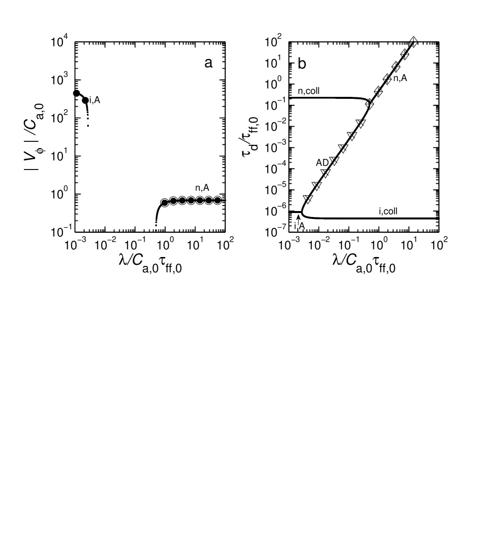
Figure 11: Eigenvalues of transverse modes as functions of wavelength, at an angle of propagation $\theta=80^{\circ}$ with respect to $\mbox{\boldmath$B$}_{0}$. All normalisations, labels, and symbols are as in Fig. 8 and Table 1. There are three different modes. (a) Absolute value of phase velocity, $|{v}_{\phi}|$. (b) Damping timescales $\tau_{{}_{\rm{d}}}$.

The dispersion relation for ion Alfvén waves, obtained from equations (10f) - (10h), has solutions given by equation (24), with $\tilde{v}_{\rm{A,i,0}}\cos\theta$ replacing $\tilde{v}_{\rm{A,i,0}}$ in that expression. Thus, the two ion Alfvén waves propagate with

$$\tilde{v}_{\phi}=\pm\tilde{v}_{\rm{A,i,0}}\cos\theta\left[1-\left(\frac{\tilde{\lambda}}{\tilde{\lambda}_{\rm{A,i}}\cos\theta}\right)^{2}\right]^{1/2}$$ (59)

(see Fig. $8a$, curve labeled “i,A”). For $\tilde{\lambda}/$($\tilde{\lambda}_{\rm{A,i}}\cos\theta$) $\ll 1$, $\tilde{v}_{\phi}\simeq\pm\tilde{v}_{\rm{A,i,0}}\cos\theta=\pm 1.99\times 10^{3}$ for the typical model cloud. The $\pm$ sign denotes degeneracy with respect to the direction of propagation. The damping timescale for these waves is $2\tilde{\tau}_{{\rm{in,0}}}$ (see Fig. $8b$, curve labeled “i,A”).

Collisions with the neutrals cut off the propagation of these waves for $\tilde{\lambda}\geq\tilde{\lambda}_{\rm{A,i}}\cos\theta=1.11\times 10^{-2}$ (see Fig $8a$). For wavelengths greater than this value, each mode bifurcates into an ion collisional-decay mode and an (ion) ambipolar-diffusion mode. The damping timescale of the former mode is given by equation (27) and is shown in Figure $8b$ (curve labeled “i,A”); it is identical with $\tilde{\tau}_{{}_{\rm{d}}}$ of the normal Alfvén waves propagating along $\mbox{\boldmath$B$}_{0}$, except for the fact that $\tilde{\lambda}_{\rm{A,i}}\cos\theta$ replaces $\tilde{\lambda}_{\rm{A,i}}$ in that expression (see discussion following eq. [24]). For very large $\tilde{\lambda}$, $\tilde{\tau}_{{}_{\rm{d}}}=\tilde{\tau}_{{\rm{in,0}}}$ (see Fig. $8b$, curve labeled “i,coll”). For the ambipolar-diffusion mode (Fig. $8b$, curve labeled “AD”), the damping timescale is the same as that given by equation (28), but again $\tilde{\lambda}_{\rm{A,i}}\cos\theta$ replaces $\tilde{\lambda}_{\rm{A,i}}$; hence, for long wavelengths, it follows from equation (29a) that

$$\tilde{\tau}_{{}_{\rm{d}}}\simeq\frac{\tilde{\lambda}^{2}}{4\pi^{2}\tilde{\cal D}_{\rm{a}}\cos^{2}\theta}.$$ (60)

At small wavelengths the third mode is a low-frequency neutral collisional-decay mode, with $\tilde{v}_{{\rm i},y}\simeq 0$ (see Fig. $9b$, curve labeled “n,coll”). The purely imaginary frequency of this mode is given by equation (30), $\tilde{\omega}=-i/\tilde{\tau}_{{\rm{ni,0}}}$; hence the damping timescale is $\tilde{\tau}_{{}_{\rm{d}}}=\tilde{\tau}_{{\rm{ni,0}}}$ ($=0.226$ for the typical model cloud; see Fig. $8b$, curve labeled “n,coll”). At longer wavelengths, the motions of the neutrals and the ions become better coupled, and the neutral collisional-decay mode merges with the ion ambipolar-diffusion mode (see Fig. $8b$), as discussed in §§ 3.1.2 and § 3.2.1. For longer wavelengths, Alfvén waves in the neutrals can be sustained, as seen in Figure $8a$. The frequencies of these modes are given by equations (31a) and (31b), but with $\tilde{v}_{\rm{A,i,0}}\cos\theta$ and $\tilde{v}_{\rm{A,n,0}}\cos\theta$ replacing $\tilde{v}_{\rm{A,i,0}}$ and $\tilde{v}_{\rm{A,n,0}}$, respectively. The lower cutoff wavelength, below which these waves cannot propagate, is $\tilde{\lambda}_{\rm{A,n}}\cos\theta=1.98$. They have phase velocity

$$\tilde{v}_{\phi}=\pm\tilde{v}_{\rm{A,n,0}}\cos\theta\left[1-\left(\frac{\tilde{\lambda}_{\rm{A,n}}\cos\theta}{\tilde{\lambda}}\right)^{2}\right]^{1/2},$$ (61)

and damping timescale

$$\tilde{\tau}_{{}_{\rm{d}}}=\frac{2\tilde{\lambda}^{2}}{4\pi^{2}\tilde{\cal D}_{\rm{a}}\cos^{2}\theta}.$$ (62)

As $\tilde{\lambda}\rightarrow\infty$, $|\tilde{v}_{\phi}|\rightarrow\tilde{v}_{\rm{A,n,0}}\cos\theta=2.79$.

The components of the eigenvectors of these modes displayed in Figures $9a$ - $9d$ are qualitatively similar to those shown in Figures $5a$ - $5d$ (for transverse modes propagating along $\mbox{\boldmath$B$}_{0}$), but with (small) quantitative decrease in the values of the critical wavelengths. We therefore do not discuss them further for economy of space.

In Figures $10a$ and $10b$ we display $|\tilde{v}_{\phi}|$ and $\tilde{\tau}_{{}_{\rm{d}}}$, respectively, for the three transverse modes propagating at an angle $\theta=10^{\circ}$ with respect to the magnetic field. The qualitative solutions of the dispersion relations for these modes are the same as for those described above for propagation at an angle $\theta=45^{\circ}$. Quantitatively, the differences in Figures $10a$ - $10b$ and $8a$ - $8b$ stem from the different values of the numerical factors $\cos\theta$ and $\sin\theta$. Similarly, the magnitude of the phase velocities and the damping timescales for the transverse modes propagating at an angle $\theta=80^{\circ}$ with respect to $\mbox{\boldmath$B$}_{0}$ are shown in Figures $11a$ and $11b$. They again differ from those for $\theta=45^{\circ}$ because of the factors $\cos\theta$ and $\sin\theta$. Although qualitatively the modes at $\theta=10^{\circ}$ and $\theta=80^{\circ}$ are the same, comparison of Figures 10 and 11 reveals that the quantitative differences in the magnitude of the phase velocities and the cutoff wavelengths are substantial. Thus the critical wavelengths that determine which modes can or cannot propagate in molecular clouds are expected to be very different depending on their direction of propagation with respect to the mean magnetic field $\mbox{\boldmath$B$}_{0}$.

3.3.2 Modes with Motions in the $(x,z)$-Plane

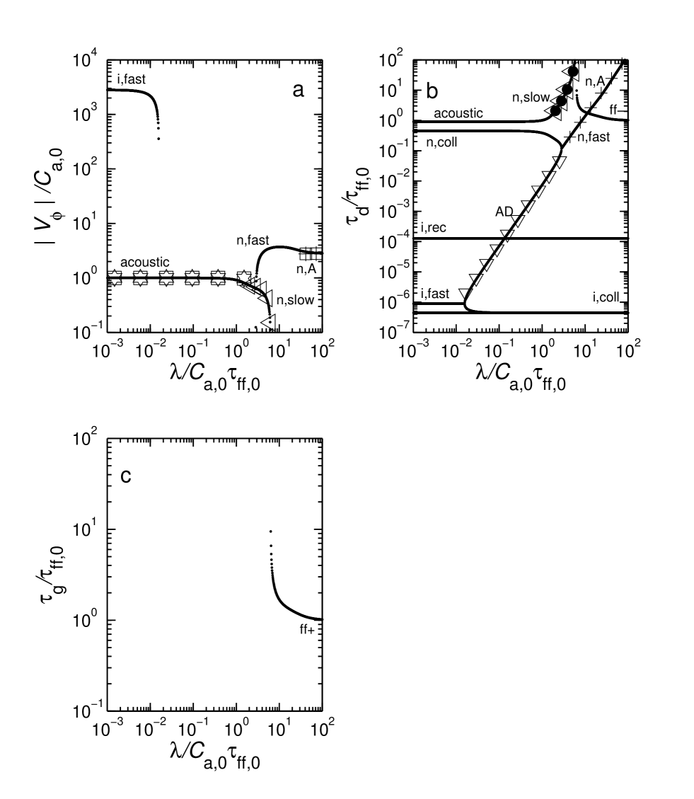
Figure 12: Eigenvalues of longitudinal modes as functions of wavelength, at an angle of propagation $\theta=45^{\circ}$ with respect to $\mbox{\boldmath$B$}_{0}$. All normalisations and labels are as in Fig. 2 and Table 1. There are seven different modes. (a) Absolute value of phase velocity, $|{v}_{\phi}|$. Boxes with interior six-pointed stars denote phase velocity values derived from eq. (66). Phase speeds calculated by using eq. (70) are shown as left-facing triangles, and phase speeds obtained from eq. (77) are shown as boxes with interior crosses. (b) Damping timescales $\tau_{{}_{\rm{d}}}$. Also displayed are values obtained from eq. (29a) (downward-facing triangles) and from eq. (71) (left-facing triangles with interior black circles). Values obtained from eq. (34a) are also displayed as crosses. (c) Growth timescale $\tau_{{}_{\rm{gr}}}$.

Figures $12a$, $12b$, and $12c$ exhibit, respectively, the magnitude of the phase velocity $\tilde{v}_{\phi}$, the damping timescale $\tilde{\tau}_{{}_{\rm{d}}}$, and the growth time $\tilde{\tau}_{{}_{\rm{gr}}}$ as functions of $\tilde{\lambda}$ for the specific case of propagation at $\theta=45^{\circ}$ with respect to $\mbox{\boldmath$B$}_{0}$ for modes with motions in the $(x,z)$-plane. Eigenvectors are displayed in Figures $13a$ - $13g$. There are 7 modes in all displayed in these figures.

As in the preceding sections, one of the ion modes is a collisional-decay mode (see Figs. $12$ and $13$, curves labeled “i,coll”), with the ions streaming through a fixed background of neutral particles ($\tilde{v}_{{\rm n},x}=\tilde{v}_{{\rm n},z}=0$); for this case $\tilde{B}_{z}=0$, and the ions move with $\tilde{v}_{{\rm i},x}=\tilde{v}_{{\rm i},z}$. The frequency is given by equation (16); hence, the damping timescale is $\tilde{\tau}_{{}_{\rm{d}}}=\tilde{\tau}_{{\rm{in,0}}}$ ($=4.45\times 10^{-7}$ for the typical model cloud). This is the horizontal line labeled by “i,coll” in Figure $12b$.

There also exist two high-frequency ion wave modes. These waves are ion fast modes. For these modes, $\tilde{v}_{{\rm i},x}/\tilde{v}_{{\rm i},z}=-\sin\!\theta/\cos\!\theta=-1$ at $\theta=45^{\circ}$ (see Figs. $13c$ and $13d$, curves labeled “i,fast”; in these Figures the “i,fast” curves coincide with the “i,coll” curves). Since the ion Alfvén speed and the magnetosonic speed (in this typical case) are essentially the same, the dispersion relation describing them is the same as equation (24); it is again the case that the waves are cut off at $\tilde{\lambda}\geq\tilde{\lambda}_{\rm{A,i}}$ ($=1.57\times 10^{-2}$ ; see Fig. $12a$). For wavelengths $>\tilde{\lambda}_{\rm{A,i}}$, each ion mode bifurcates into an ion collisional-decay mode and an ion ambipolar-diffusion mode (see Fig. $12b$). The decay timescales for these two modes are the same as those previously discussed for the cases $\theta=0^{\circ}$ and $90^{\circ}$ (see § 3.1.2 and § 3.2.1).

The fourth mode is the ion dissociative-decay mode, discussed previously in §§ 3.1.1 and 3.2.1. In this mode, nonpropagating density perturbations in the ions decay by dissociative recombinations of molecular ions and electrons. The decay time is $\tilde{\tau}_{{}_{\rm{d}}}=\left(2\tilde{\rho}_{\rm{i,0}}\tilde{\alpha}_{\rm{m,dr}}\right)^{-1}$ ($=1.28\times 10^{-4}$ for the typical model cloud); this is the horizontal line labeled by “i,rec” in Figure $12b$.

At small wavelengths there are two low-frequency acoustic-wave modes in the neutrals and one neutral collisional-decay mode. The dispersion relation for the acoustic modes, which are predominantly polarised in the $x$-direction, is most easily found by first finding $\tilde{v}_{{\rm i},x}$ in terms of $\tilde{v}_{{\rm n},x}$ and $\tilde{\omega}$. In the limit $|\tilde{\omega}|\ll 1/\tilde{\tau}_{{\rm{in,0}}}$ and $\tilde{\omega}\tilde{B}_{z}\simeq 0$, one finds from equations (10i), (10j), (10k), and (10d) that

$$\tilde{v}_{{\rm i},x}\simeq\tilde{v}_{{\rm n},x}\cos^{2}\theta\left[\frac{\tilde{\omega}+\left(i/\tilde{\tau}_{{\rm{ni,0}}}\right)}{\tilde{\omega}+\left(i\cos^{2}\theta/\tilde{\tau}_{{\rm{ni,0}}}\right)}\right].$$ (63)

For $|\tilde{\omega}|\ga 1/\tilde{\tau}_{{\rm{ni,0}}}$, the term in brackets in equation (63) is essentially unity, and $\tilde{v}_{{\rm i},x}\simeq\tilde{v}_{{\rm n},x}\cos^{2}\!\theta$. The factor $\cos^{2}\!\theta$ is a measure of the opposition presented to the neutrals by the ions, which are attached to magnetic field lines. If $\theta=0^{\circ}$ the ions are effectively inertialess, and the neutrals sweep them up easily, so that $\tilde{v}_{{\rm i},x}=\tilde{v}_{{\rm n},x}$. However, if $\theta=90^{\circ}$, $\tilde{v}_{{\rm i},x}\simeq 0$, i.e., the ions are held in place by the magnetic field as the neutrals move through them. In this case, the ions present the stiffest opposition to the neutral motion. For $|\tilde{\omega}|\ga 1/\tilde{\tau}_{{\rm{ni,0}}}$, we insert equation (63) in equation (10c) to find the solution

$$\tilde{\omega}=\pm\tilde{k}\left\{1-\frac{1}{\tilde{k}^{2}}\left[1+\left(\frac{\sin^{2}\theta}{2\tilde{\tau}_{{\rm{ni,0}}}}\right)^{2}\right]\right\}^{1/2}-i\frac{\sin^{2}\theta}{2\tilde{\tau}_{{\rm{ni,0}}}}.$$ (64)

[Note that for $\theta=0^{\circ}$ or $90^{\circ}$, equation (64) reduces to equations (18) or (44), respectively.] For

$$\tilde{\lambda}\la\frac{\tilde{\lambda}_{\rm{s,n}}}{{\cal A}_{\rm{s,n}}(\theta)}~{}~{},$$ (65a)

where

$${\cal A}_{\rm{s,n}}(\theta)\equiv\left[\frac{\sin^{4}\theta+(2\tilde{\tau}_{{\rm{ni,0}}})^{2}}{1+(2\tilde{\tau}_{{\rm{ni,0}}})^{2}}\right]^{1/2}~{}~{},$$ (65b)

these modes are sound waves, with

$$\tilde{v}_{\phi}=\pm\left[1-\left(\frac{\tilde{\lambda}{\cal A}_{\rm{s,n}}(\theta)}{\tilde{\lambda}_{\rm{s,n}}}\right)^{2}\right]^{1/2}$$ (66)

(see Fig. $12a$) and $\tilde{\tau}_{{}_{\rm{d}}}=2\tilde{\tau}_{{\rm{ni,0}}}/\sin^{2}\theta=0.904$ for $\theta=45^{\circ}$ (see horizontal line labeled “acoustic” in Fig. $12b$). ${\cal A}_{\rm{s,n}}(\theta)$ is the acoustic-wave angular (or, stiffness) parameter: for $\theta=90^{\circ}$ equations (65a) and (66) yield our earlier result, that sound waves propagate only for $\tilde{\lambda}\leq\tilde{\lambda}_{\rm{s,n}}$, while for $\theta=0^{\circ}$ we recover our other earlier result that $\tilde{\lambda}_{\rm{J,th}}$ is the upper cutoff wavelength for these waves.

The sound-wave upper cutoff wavelength (65a) is relevant only if the waves do not transition into neutral slow modes at larger wavelengths (see discussion below). It turns out that this depends on the angle $\theta$ of propagation: the upper cutoff equation is applicable only to sound waves propagating at $\theta>\theta_{\rm{max}}$ (for the typical model cloud, $\theta_{\rm{max}}=62.9^{\circ}$ — see below). For sound waves propagating at such angles, there is a mode bifurcation at the cutoff (65a). The dispersion relation (64) reveals that at larger $\tilde{\lambda}$ one of the modes becomes a neutral collisional-decay mode, with damping timescale $\tilde{\tau}_{{}_{\rm{d}}}\rightarrow\tilde{\tau}_{{\rm{ni,0}}}/\sin^{2}\theta$, and the other mode becomes a pressure-driven diffusion mode with damping timescale

$$\tilde{\tau}_{{}_{\rm{d}}}=\frac{(\tilde{\lambda}/\tilde{\lambda}_{\rm{J,th}})^{2}\sin^{2}\theta}{\tilde{\cal D}_{\rm{P}}[1-(\tilde{\lambda}/\tilde{\lambda}_{\rm{J,th}})^{2}]}\,\,\,\,\,\,\,\,\,\,{\rm for}\,\,\,\tilde{\lambda}\,\leq\,\tilde{\lambda}_{\rm{J,th}}~{}.$$ (67)

This diffusion timescale is the same as that of equation (47a), except that it is multiplied by $\sin^{2}\theta$, which reflects the reduced effectiveness of neutral-ion collisions in slowing down the neutrals at angles $\theta<90^{\circ}$ with respect to the magnetic field. At $\tilde{\lambda}=\tilde{\lambda}_{\rm{J,th}}$ the timescale (67) becomes infinite. For $\tilde{\lambda}>\tilde{\lambda}_{\rm{J,th}}$ there is a neutral ambipolar-diffusion–induced gravitational fragmentation mode at the angle $\theta$ ($>\theta_{\rm{max}}$), having a growth time

$$\tau_{{}_{\rm{gr}}}=\frac{\sin^{2}\theta/\tilde{\tau}_{{\rm{ni,0}}}}{1-\left(\tilde{\lambda}_{\rm{J,th}}/\tilde{\lambda}\right)^{2}}=\frac{\nu_{\rm{ff},0}\sin^{2}\theta}{1-\left(\tilde{\lambda}_{\rm{J,th}}/\tilde{\lambda}\right)^{2}}~{}~{}.$$ (68)

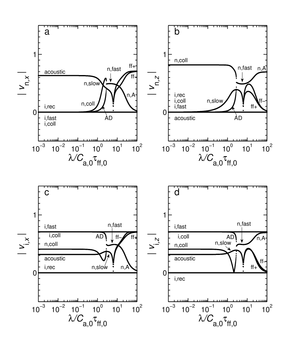
Figure 13: Magnitudes of eigenvectors of modes with motions in the (x,z)-plane for $\theta=45^{\circ}$ as functions of wavelength. All labels and normalisations are the same as in Fig. 3 and Table 1. As in Fig. 12, there are seven modes. (a) Longitudinal ($x$-)component of the neutral velocity, $|v_{{\rm n},x}|$; (b) $|v_{{\rm n},z}|$. (c) Longitudinal ($x$-)component of the ion velocity, $|v_{{\rm i},x}|$; (d) $|v_{{\rm i},z}|$.

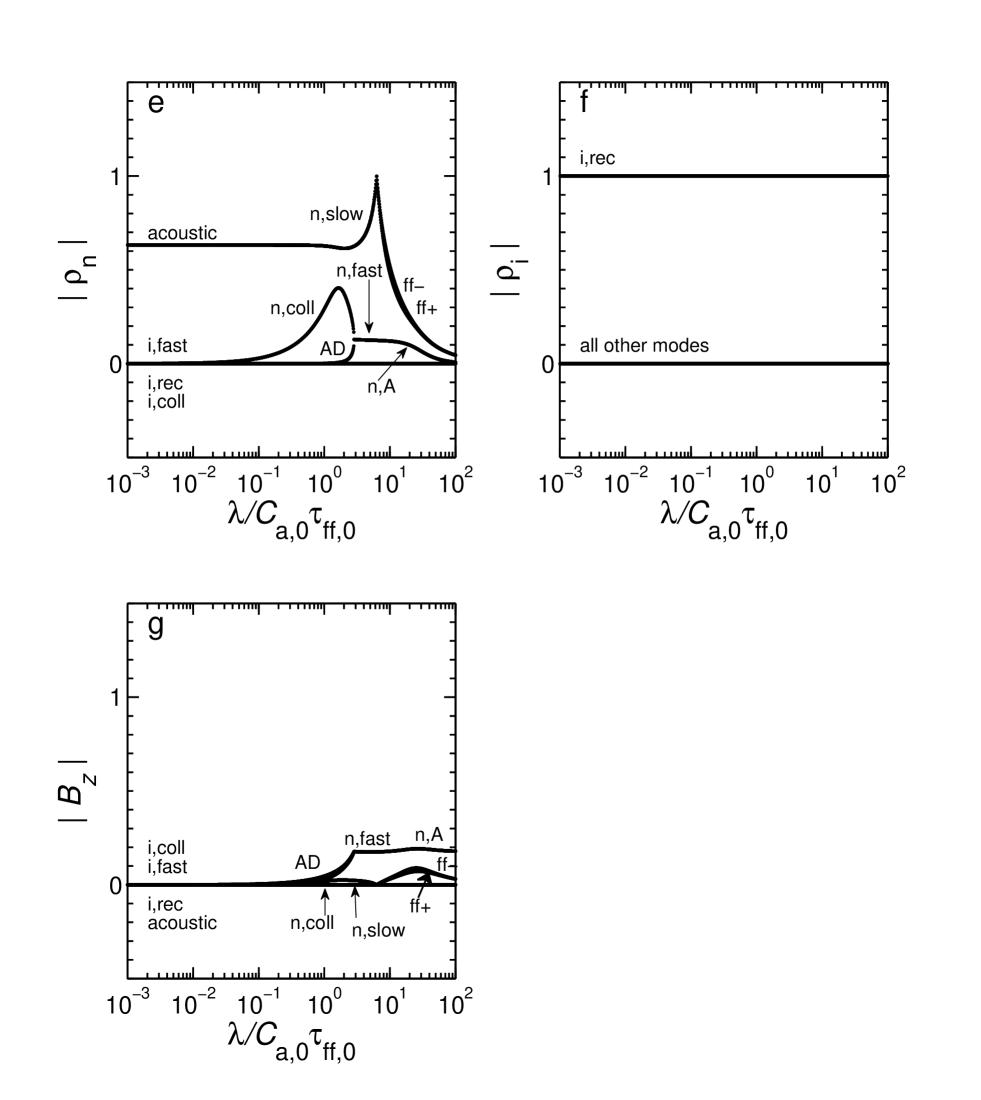
Figure 13: Cont. (e) Neutral density $|\rho_{\rm n}|$. (f) Ion density $|\rho_{\rm i}|$. (g) Magnetic field component $|B_{z}|$.

The fragmentation time (68) is equal to the growth time (49) multiplied by $\sin^{2}\theta$, again reflecting the reduced collisional resistance on the neutrals by magnetically-coupled ions when the angle of propagation is less than $90^{\circ}$ with respect to the field direction. For $\tilde{\lambda}\gg\tilde{\lambda}_{\rm{J,th}}$, equation (68) yields $\tilde{\tau}_{{}_{\rm{gr}}}\rightarrow\sin^{2}\theta/\tilde{\tau}_{{\rm{ni,0}}}=\nu_{\rm{ff},0}\sin^{2}\theta$. However, similar to what occurs in the case for $\theta=90^{\circ}$ (see § 3.2.1 and Fig. $5c$), this limit will not be attained because the approximation of stationary field lines breaks down when $\tilde{\lambda}$ becomes $\ga\tilde{\lambda}_{\rm{J,mag}}$. When this happens, magnetic forces are overwhelmed by self-gravitational forces and $\tau_{{}_{\rm{gr}}}\rightarrow 1$ at these larger wavelengths.

From equation (64) one finds that collisional damping of the motion of the neutrals by ions causes $|\tilde{v}_{\phi}|$ to become less than unity for $\tilde{\lambda}$ near the value given by the right-hand side of equation (65a). However, for $0<\theta<90^{\circ}$, the sound waves are not always cut off at this wavelength. This is due to the fact that the bracketed term in the expression for the $x$-component of the ion velocity (eq. [63]) is no longer essentially unity (because $|\tilde{\omega}|\sim 1/\tilde{\tau}_{{\rm{ni,0}}}$) at these wavelengths; thus, the dispersion relation (64) is no longer valid. Physically, this is a result of the fact that the ions move readily with the neutrals in the $x$-direction at these frequencies; this means that the waves suffer less damping, because the frictional force on the neutrals is reduced when the ions and the neutrals move together. (We note that, for $\theta<90^{\circ}$, equation [63] yields $\tilde{v}_{{\rm i},x}\simeq\tilde{v}_{{\rm n},x}$ in the limit $|\tilde{\omega}|\ll 1/\tilde{\tau}_{{\rm{ni,0}}}$.)

For $\tilde{\lambda}$ sufficiently large, such that $|\tilde{\omega}|\la\cos^{2}\theta/\tilde{\tau}_{{\rm{ni,0}}}$, the frequency of the neutral waves is

$$\tilde{\omega}\simeq\pm\tilde{k}\cos\theta\left\{\left(1-\frac{1}{\tilde{k}^{2}}\right)\left[1-\left(\frac{\tilde{\tau}_{{\rm{ni,0}}}\tilde{k}\sin\theta\tan\theta}{2}\right)^{2}\left(1-\frac{1}{\tilde{k}^{2}}\right)\right]\right\}^{1/2}-\frac{i}{2}\tilde{\tau}_{{\rm{ni,0}}}\left(\tilde{k}^{2}-1\right)\sin^{2}\theta~{}~{}.$$ (69)

Hence, for these conditions, the phase velocity is

$$\tilde{v}_{\phi}=\pm\cos\theta\left\{\left(1-\frac{\tilde{\lambda}^{2}}{\tilde{\lambda}_{\rm{J,th}}^{2}}\right)\left[1-\left(\frac{\tilde{\lambda}_{\rm{s,n}}\sin\theta\tan\theta}{4\tilde{\lambda}}\right)^{2}\left(1+4\tilde{\tau}_{{\rm{ni,0}}}^{2}\right)\left(1-\frac{\tilde{\lambda}^{2}}{\tilde{\lambda}_{\rm{J,th}}^{2}}\right)\right]\right\}^{1/2},$$ (70)

and

$$\tilde{\tau}_{{}_{\rm{d}}}=\frac{2(\tilde{\lambda}/\tilde{\lambda}_{\rm{J,th}})^{2}}{\tilde{\cal D}_{\rm{P}}\left[1-\left(\tilde{\lambda}/\tilde{\lambda}_{\rm{J,th}}\right)^{2}\right]\sin^{2}\theta}.$$ (71)

These waves are neutral slow modes, modified by gravity, and cannot propagate at wavelengths $\tilde{\lambda}\geq\tilde{\lambda}_{\rm{J,th}}$ ($=2\pi$ for the typical model cloud); at $\theta=0^{\circ}$ the slow mode dispersion relation (69) is identical to the relation for the Jeans mode (eq. [18]). From the low-frequency condition used to derive equation (69) it is found that slow modes exist only for wavelengths

$$\tilde{\lambda}\,\ga\,\tilde{\lambda}_{\rm{s,n}}{\cal S}_{\rm{n}}(\theta)~{},$$ (72a)

where

$${\cal S}_{\rm{n}}(\theta)\equiv\frac{\left[1+(2\tilde{\tau}_{{\rm{ni,0}}})^{2}\right]^{1/2}}{2|\cos\theta|}~{},$$ (72b)

provided that

$${\cal A}_{\rm{s,n}}(\theta){\cal S}_{\rm{n}}(\theta)\,\la\,1~{}.$$ (73)

The quantity ${\cal S}_{\rm{n}}(\theta)$ is the angular slow-mode factor. The relation (73) is derived from the requirement that the slow modes arise from the acoustic wave modes. For this mode conversion to occur, the minimum slow mode wavelength (72a) must be less than or equal to the acoustic-wave upper cutoff wavelength (65a); thus, the inequality (73) follows. This is equivalent to having $\theta\leq\theta_{\rm{max}}$, where $\theta_{\rm{max}}$ is defined by the condition

$$\frac{\cos^{2}\theta_{\rm{max}}}{\sin^{4}\theta_{\rm{max}}+(2\tilde{\tau}_{{\rm{ni,0}}})^{2}}=\frac{1}{4}~{}~{}.$$ (74)

If $\theta\leq\theta_{\rm{max}}$, slow modes emerge from the acoustic modes (without a bifurcation) and propagate for $\tilde{\lambda}_{\rm{s,n}}{\cal S}_{\rm{n}}(\theta)\la\tilde{\lambda}\leq\tilde{\lambda}_{\rm{J,th}}$. Otherwise, when $\theta>\theta_{\rm{max}}$, the acoustic waves have an upper cutoff and mode bifurcation occurs at the wavelength (65a); in that case, there are no slow modes.

For the typical model cloud, with $\tilde{\tau}_{{\rm{ni,0}}}=0.226$, $\theta_{\rm{max}}=62.9^{\circ}$. At $\theta=45^{\circ}$ the slow mode minimum wavelength $\tilde{\lambda}_{\rm{s,n}}{\cal S}_{\rm{n}}(45^{\circ})=2.01$, and the transition from sound waves to slow modes can be seen in Figures $12a$ and $12b$ (curves labeled “n,slow”) to occur at this wavelength; Figures $13a$ and $13c$ show that, for these modes, $\tilde{v}_{{\rm n},x}\simeq\tilde{v}_{{\rm i},x}$ at wavelengths greater than or equal to the transition wavelength.

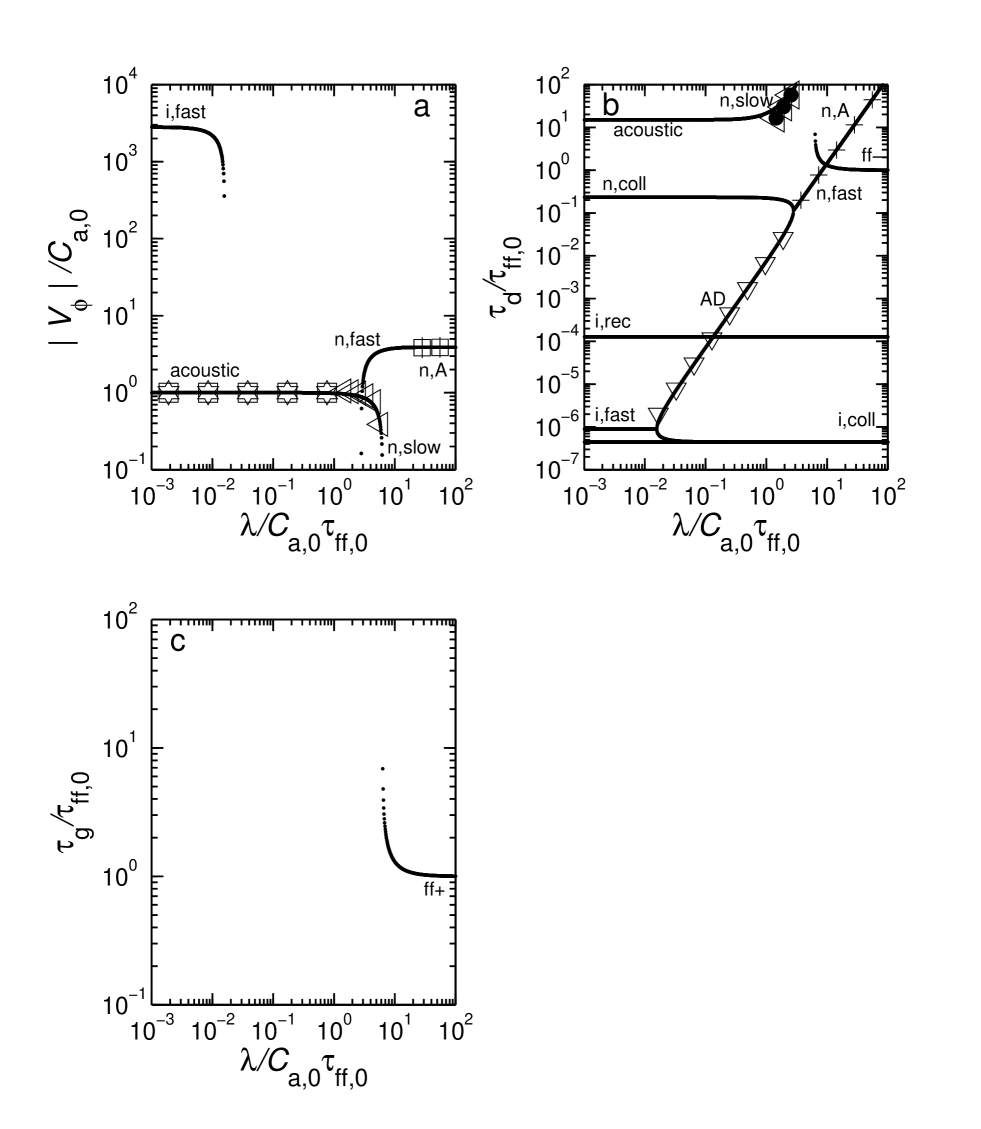
Figure 14: Eigenvalues of longitudinal modes as functions of wavelength, at an angle of propagation $\theta=10^{\circ}$ with respect to $\mbox{\boldmath$B$}_{0}$. All normalisations, labels, and symbols are as in Fig. 12 and Table 1. There are seven different modes. (a) Absolute value of phase velocity, $|{v}_{\phi}|$. (b) Damping timescales $\tau_{{}_{\rm{d}}}$. (c) Growth timescale $\tau_{{}_{\rm{gr}}}$.

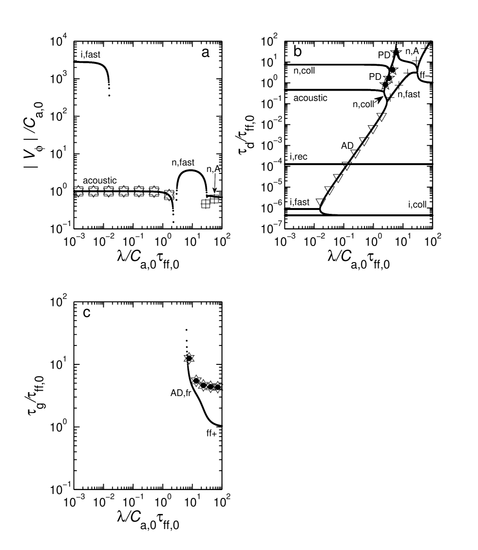
Figure 15: Eigenvalues of longitudinal modes as functions of wavelength, at an angle of propagation $\theta=80^{\circ}$ with respect to $\mbox{\boldmath$B$}_{0}$. All normalisations, labels, and symbols are as in Fig. 12 and Table 1. There are seven different modes. (a) Absolute value of phase velocity, $|{v}_{\phi}|$. (b) Damping timescales $\tau_{{}_{\rm{d}}}$. Five-pointed stars with interior black circles represent values calculated by using eq. (67). (c) Growth timescale $\tau_{{}_{\rm{gr}}}$. Values obtained from eq. (68) are depicted as six-pointed stars with interior black circles.

Note that, as $\tilde{\lambda}\rightarrow\tilde{\lambda}_{\rm{J,th}}$ from below, equation (71) shows that the slow mode damping timescale $\tilde{\tau}_{{}_{\rm{d}}}\rightarrow\infty$ (see curve labeled by “n,slow” in Fig. $12b$). For $\tilde{\lambda}>\tilde{\lambda}_{\rm{J,th}}$ there are again the two conjugate modes: the gravitational instability (or Jeans) mode (see Fig. $12c$, curve labeled “ff+”) and the “cosmological” mode (see curve labeled “ff$-$” in Fig. $12b$; although this curve “crosses” the curve labeled “n,fast” in Fig. $12b$, the two modes do not actually interact); as $\tilde{\lambda}\rightarrow\infty$, both the growth timescale of the unstable mode and the damping timescale of the cosmological mode go to unity (i.e., in dimensional form, $\tau_{\rm{gr}}=\tau_{\rm{d}}=\tau_{{}_{\rm{ff,0}}}$), as seen in Figures $12b$ and $12c$, respectively.

The other mode affecting the neutrals at short wavelengths is a neutral collisional-decay mode (“n,coll”). The velocity of the neutrals at small $\tilde{\lambda}$ is predominantly in the $z$-direction for this mode (see Figs. $13a$ and $13b$); the frequency is purely imaginary and given by

$$\tilde{\omega}=-i\frac{\cos^{2}\theta}{\tilde{\tau}_{{\rm{ni,0}}}}.$$ (75)

Thus, $\tilde{\tau}_{{}_{\rm{d}}}=\tilde{\tau}_{{\rm{ni,0}}}/\cos^{2}\theta=0.452$ (see Fig. $12b$, curve labeled “n,coll”). For $\tilde{\lambda}$ greater than the value given by the right-hand side of equation (65a), it is again the case that the motion of the ions and magnetic field becomes better coupled to that of the neutrals. In this wavelength regime $|\tilde{v}_{{\rm n},x}|\simeq|\tilde{v}_{{\rm n},z}|\simeq|\tilde{v}_{{\rm i},x}|\simeq|\tilde{v}_{{\rm i},z}|$ (see Figs. $13a$ - $13d$). This mode merges with the ion ambipolar-diffusion mode at $\tilde{\lambda}=\tilde{\lambda}_{\rm{ms,n}}$ (see Fig. $12b$), and, for $\tilde{\lambda}>\tilde{\lambda}_{\rm{ms,n}}$, fast modes are excited in the neutrals (curves labeled “n,fast” in Figs. $12a,12b$, and $13a$ - $13d$), degenerate with respect to the direction of propagation. In these modes, the polarisation is given by $\tilde{v}_{{\rm n},x}/\tilde{v}_{{\rm n},z}=-\sin\!\theta/\cos\!\theta$ ($=-1$ for $\theta=45^{\circ}$). Hence, $\tilde{\mbox{\boldmath$v$}}_{\rm n}\cdot\mbox{\boldmath$B$}_{0}=0$, i.e., the fast modes are polarised perpendicular to the magnetic field. The dispersion relation for these modes is essentially the same as equation (51) because of the fact that $\tilde{v}_{\rm{A,n,0}}^{2}\gg 1$. They decay, as they propagate, on the ambipolar-diffusion timescale (see Fig. $12b$). For $\tilde{\lambda}\geq\tilde{\lambda}_{\rm{J,mag}}$, these waves tend to get suppressed by gravity.

For $\tilde{\lambda}>\tilde{\lambda}_{\rm{J,mag}}$ thermal and magnetic restoring forces in the $x$-direction are overwhelmed by gravitational forces, making $\tilde{v}_{{\rm n},x}\simeq 0$ (see Fig. $13a$). Hence the modes become essentially incompressible. Waves are still able to propagate for longer wavelengths, however, because of the transverse restoring magnetic tension force (i.e., $\tilde{B}_{z}\neq 0$; see Fig. $13g$). Solving equations (10a) - (10d) and (10i) - (10k) with the conditions $\tilde{v}_{{\rm n},x}=0=\tilde{\rho}_{\rm n}$ in the limit $|\tilde{\omega}|\ll 1/\tilde{\tau}_{{\rm{in,0}}}$, we find

$$\tilde{\omega}=\pm\tilde{v}_{\rm{A,n,0}}\tilde{k}\cos\theta\left[1-\left(\frac{\tilde{v}_{\rm{A,n,0}}\tilde{\tau}_{{\rm{ni,0}}}\tilde{k}}{2\cos\!\theta}\right)^{2}\right]^{1/2}-\frac{i}{2}\tilde{v}_{\rm{A,n,0}}^{2}\tilde{\tau}_{{\rm{ni,0}}}\tilde{k}^{2}.$$ (76)

Hence, these modes are modified Alfvén waves in the neutrals, with

$$\tilde{v}_{\phi}=\pm\tilde{v}_{\rm{A,n,0}}\cos\theta\left[1-\left(\frac{\tilde{\lambda}_{\rm{A,n}}}{\tilde{\lambda}\cos\theta}\right)^{2}\right]^{1/2}$$ (77)

and $\tilde{\tau}_{{}_{\rm{d}}}=2\tilde{\lambda}^{2}/4\pi^{2}\tilde{\cal D}_{\rm{a}}$. In the limit $\tilde{\lambda}\rightarrow\infty$, $|\tilde{v}_{\phi}|\simeq\tilde{v}_{\rm{A,n,0}}\cos\theta=2.79$, in agreement with the long-wavelength behaviour of these modes shown in Figure $12a$ (curves labeled “n,fast” and “n,A”). This is yet another example of a transition between wave modes without bifurcation.

Figures $14a$, $14b$, and $14c$ show $|\tilde{v}_{\phi}|$, $\tilde{\tau}_{{}_{\rm{d}}}$, and $\tilde{\tau}_{{}_{\rm{gr}}}$ as functions of $\tilde{\lambda}$ for the seven different modes with motions in the ($x,z$)-plane propagating at an angle $\theta=10^{\circ}$ with respect to $\mbox{\boldmath$B$}_{0}$. Comparison with Figures $12a$ - $12c$ reveals that the qualitative behaviour of the various modes as functions of wavelength is the same as in the case of propagation at $\theta=45^{\circ}$. The quantitative differences stem from the numerical factors $\cos\theta$ and $\sin\theta$, which become substantial for $\theta$ approaching $0^{\circ}$ or $90^{\circ}$. As Figure $14a$ shows clearly, wave modes in the neutrals exist at all wavelengths and their decay times are very long (see Fig. $14b$, curves labeled “acoustic”, “n,slow”, and “n,fast”). Figures $15a$, - $15c$ show the same quantities as Figures $14a$ - $14c$ but for propagation at $\theta=80^{\circ}$ with respect to the unperturbed magnetic field $\mbox{\boldmath$B$}_{0}$. There are no slow modes in Figure 15 (unlike the cases in Figs. 12 and 14) because $\theta>\theta_{\rm{max}}$ for that angle of propagation in the typical model. Instead, the sound waves are cut off at the maximum wavelength $\tilde{\lambda}=\tilde{\lambda}_{\rm{s,n}}/{\cal A}_{\rm{s,n}}(80^{\circ})=2.66$, where there is a bifurcation. At wavelengths greater than this maximum, the modes are a pressure-driven diffusion mode (“PD” curve) and a neutral collisional-decay mode (“n,coll”). There is also an ambipolar diffusion-induced fragmentation mode seen in Figure $15c$ (“AD,fr” curve), which approaches the predicted limiting value (see eq. [68]) of $\sin^{2}80^{\circ}/\tilde{\tau}_{{\rm{ni,0}}}=4.29$ at $\tilde{\lambda}$ just below $\tilde{\lambda}_{\rm{J,mag}}$ (= 25.6 in the typical model cloud).

4 SUMMARY AND DISCUSSION

We have obtained and analyzed the dispersion relations for MHD wave modes and instabilities for different directions of propagation with respect to the zeroth-order magnetic field $\mbox{\boldmath$B$}_{0}$ in a two-fluid weakly ionised system, and we have applied the results to a typical interstellar molecular cloud. The system of equations has four dimensionless free parameters, $\tilde{\tau}_{{\rm{ni,0}}}$, $\tilde{\tau}_{{\rm{in,0}}}$, $\tilde{v}_{\rm{A,i,0}}$, and $\tilde{\alpha}_{\rm{m,dr}}$. They represent, respectively, the neutral-ion (momentum-exchange) collision time and the ion-neutral collision time in units of the free-fall time of the zeroth-order state, the Alfvén speed in the ions in units of the adiabatic speed of sound in the neutrals, and the dissociative recombination coefficient (see eq. [11d]). (Because of ionisation equilibrium in the zeroth-order state, the dimensionless cosmic-ray ionisation rate $\tilde{\zeta}_{{}_{\rm{CR}}}$ is expressible in terms of $\tilde{\alpha}_{\rm{m,dr}}$, $\tilde{\tau}_{{\rm{in,0}}}$ and $\tilde{\tau}_{{\rm{ni,0}}}$.)

There are two distinct kinds of ambipolar diffusion, whose combined effect is unavoidable in typical molecular clouds and has crucial consequences on their evolution:

• In the presence of hydromagnetic (HM) waves or turbulence, the tension of field lines (or the outward pressure due to compressed field lines) drives the motion of charged particles relative to the neutrals, with the tendency/consequence to straighten out the bent or tangled magnetic field lines (or to move compressed field lines apart, toward a more uniform configuration). The timescale of this process is proportional to the square of the wavelength of the HM waves (or the characteristic length of the field-line tangling, or the magnitude of the field gradient) – see eqs. (34a) and (80). For lengthscales typical of molecular cloud cores ($\la\,0.1$ pc), it is much smaller than the free-fall time. This is the magnetically-driven ambipolar diffusion. It is this kind of ambipolar diffusion which is responsible for the observed large-scale ordering of polarisation vectors, indicating large-scale ordering of the magnetic field lines in molecular clouds.
  

• Gravitationally-driven ambipolar diffusion sets in with a short enough timescale, but longer than the free-fall time, in the deep interiors of self-gravitating clouds, where the degree of ionisation is $x_{\rm i}\la 10^{-7}$. Its onset can be spontaneous or initiated as a result of magnetically-driven ambipolar diffusion depriving a self-gravitating cloud of any support that most short-wavelength HM waves (or turbulence) may have provided against the cloud’s self-gravity (Mouschovias 1987a). It (i) allows the clouds to fragment as neutral particles contract through almost stationary field lines (and the attached charged particles); and, consequently, (ii) increases the mass-to-flux ratio of the forming fragments (or cores). Once the critical mass-to-flux ratio (Mouschovias & Spitzer 1976) of fragments is exceeded, dynamical contraction ensues, while the cloud envelopes remain magnetically supported, as found by numerical simulations starting with Fiedler & Mouschovias (1993) and confirmed by numerous observations.

Hydromagnetic (HM) waves with phase velocity

$$|v_{\phi}|\simeq v_{\rm{A,n,0}}=0.96\left(\frac{B_{0}}{30~{}\mu\rm{G}}\right)\left(\frac{2\times 10^{3}~{}\rm{cm}^{-3}}{n_{\rm{n,0}}}\right)^{1/2}\,\,\,\,\,\rm{km}~{}\rm{s}^{-1},$$ (78)

can propagate in all directions with respect to $\mbox{\boldmath$B$}_{0}$, provided that $\lambda\ga\lambda_{\rm{A,n}}$, where

$$\lambda_{\rm{A,n}}=\pi v_{\rm{A,n,0}}\tau_{{\rm{ni,0}}}=0.22\left(\frac{B_{0}}{30~{}\mu\rm{G}}\right)\left(\frac{2\times 10^{3}~{}\rm{cm}^{-3}}{n_{\rm{n,0}}}\right)^{3/2}\left(\frac{2\times 10^{-7}}{x_{\rm i,0}}\right)\,\,\,\,\,\rm{pc}.$$ (79)

The long-wavelength waves are long-lived; the decay time is the magnetically-driven ambipolar-diffusion timescale

$$\tau_{\rm{d}}\simeq\frac{\lambda^{2}}{2\pi^{2}v_{\rm{A,n,0}}^{2}\tau_{{\rm{ni,0}}}}=7.5\times 10^{5}\left(\frac{\lambda}{1~{}\rm{pc}}\right)^{2}\left(\frac{30~{}\mu{\rm G}}{B_{0}}\right)^{2}\left(\frac{n_{\rm{n,0}}}{2\times 10^{3}~{}{\rm{cm}^{-3}}}\right)^{2}\left(\frac{x_{\rm i,0}}{2\times 10^{-7}}\right)\,\,\,\,\,\rm{yr,}$$ (80)

which is to be distinguished from the growth time of gravitationally-driven ambipolar-diffusion, relevant to fragmentation of molecular clouds into self-gravitating cores; namely,

$$\tau_{\rm AD,fr}=\frac{{\tau_{{}_{\rm{ff,0}}}}^{2}}{\tau_{\rm ni,0}}\simeq 1.1\times 10^{6}\,\left(\frac{x_{\rm i,0}}{10^{-7}}\right)\,\,\,\,\,\rm{yr}.$$ (81)

The (one-dimensional) free-fall timescale at the density $n_{\rm{n,0}}=2\times 10^{3}\,\rm{cm}^{-3}$ as $\lambda\rightarrow\infty$ is $\tau_{{}_{\rm{ff,0}}}=(4\pi G\rho_{\rm n,0})^{-1/2}=3.9\times 10^{5}$ yr. The nonlinear counterparts of these modes have been shown to explain quantitatively the observed highly supersonic but subAlfvénic linewidths in molecular clouds, their cores, and even in OH and H₂O masers in which the strength of the magnetic field has been measured (Mouschovias & Psaltis 1995; Mouschovias et al. 2006).

Most HM waves with $\lambda<\lambda_{\rm{A,n}}$ cannot propagate in the neutrals because they are damped rapidly by ambipolar diffusion. This means that there cannot be any contribution from this wavelength regime to the spectrum of HM “turbulence” in molecular clouds (Mouschovias & Psaltis 2011, in preparation), which may provide clouds with a source of nonthermal pressure. This led Mouschovias (1987a) to argue that the decay of HM waves by ambipolar diffusion on wavelength scales $\la 0.1-0.3~{}\rm{pc}$ can initiate the formation of protostellar cores in otherwise magnetically supported clouds (see also Mouschovias 1991a). Damping of short-wavelength HM waves by ambipolar diffusion has also been proposed (Mouschovias 1987a, § 2.2.5) as the cause of the observed narrowing and thermalization of linewidths with increasing column density, as observed, for example, by Baudry et al. (1981) in the cloud TMC 2. Depending on the angle of propagation with respect to the unperturbed magnetic field $\mbox{\boldmath$B$}_{0}$, however, we find that certain long-lived modes in the neutrals exist at all wavelengths, while ion modes usually damp very rapidly even at short wavelengths. This may explain the observations by Li & Houde (2008) in the M17 molecular cloud, which show neutral motions at small lengthscales but much smaller ion motions on the same scales.

Gravitational instability is found to set in at $\lambda=\lambda_{\rm J,th}$ (the thermal Jeans wavelength) for all $\theta$, in agreement with Chandrasekhar & Fermi (1953). For $\theta\simeq 90^{\circ}$, though, the timescale for the instability is $\simeq\nu_{\rm{ff},0}\tau_{{}_{\rm{ff,0}}}=\tau_{{}_{\rm{ff,0}}}^{2}/\tau_{{\rm{ni,0}}}$, which is the gravitationally-driven ambipolar-diffusion timescale. This is in agreement with the result for the ambipolar-diffusion–initiated formation and contraction of protostellar fragments (or cores) obtained from nonlinear calculations analytically by Mouschovias (1979, 1989) and Mouschovias & Paleologou (1986), and numerically by Fiedler & Mouschovias (1993) for a two-fluid system (neutral molecules and plasma), Ciolek & Mouschovias (1994) for a four-fluid system (i.e., neutral molecules, plasma, negatively-charged, and neutral grains) , and Basu & Mouschovias (1994, 1995a, b) for a two-fluid system including rotation and magnetic braking. It is also in agreement with the results of simulations by Tassis & Mouschovias (2007a, b, c) and Kunz & Mouschovias (2009, 2010) for a six-fluid system (neutral molecules, atomic and molecular ions, electrons, negatively-charged, positively-charged, and neutral grains).

Another recent success of the linear theory (applied to model molecular clouds flattened along the magnetic field) in predicting inherently nonlinear phenomena was demonstrated by Kunz & Mouschovias (2010). They obtained analytically the Core Mass Function (CMF) resulting from gravitationally-driven ambipolar-diffusion–induced fragmentation of molecular clouds. The predicted CMF is in excellent agreement with observations of more than 300 cores in Orion (Nutter & Ward-Thompson 2007), not only at the high-mass end (for which many alternative models can obtain such agreement), but also at the turnover mass and low-mass end.

Table 2: Critical Wavelengths

	Dimensionless Expression	Model Value†	Dimensional Expression
ion Alfvén-wave upper cutoff	$\tilde{\lambda}_{\rm{A,i}}=4\pi\tilde{v}_{\rm{A,i,0}}\tilde{\tau}_{{\rm{in,0}}}$	0.0157	$\lambda_{\rm{A,i}}=4\pi v_{\rm{A,i,0}}\tau_{{\rm{in,0}}}$
ion magnetosonic-wave upper cutoff	$\tilde{\lambda}_{\rm{A,i}}$	0.0157	$\lambda_{\rm{A,i}}$
acoustic-wave upper cutoff	$\tilde{\lambda}_{\rm{s,n}}=4\pi\tilde{\tau}_{{\rm{ni,0}}}/[1+(2\tilde{\tau}_{{\rm{ni,0}}})^{2}]^{1/2}$	2.59	$\lambda_{\rm{s,n}}=4\pi C_{\rm{a},0}\tau_{{\rm{ni,0}}}/[1+(2\tilde{\tau}_{{\rm{ni,0}}})^{2}]^{1/2}$
neutral Alfvén-wave lower cutoff	$\tilde{\lambda}_{\rm{A,n}}=\pi\tilde{v}_{\rm{A,n,0}}\tilde{\tau}_{{\rm{ni,0}}}$	2.80	$\lambda_{\rm{A,n}}=\pi v_{\rm{A,n,0}}\tau_{{\rm{ni,0}}}$
neutral magnetosonic-wave lower cutoff	$\tilde{\lambda}_{\rm{ms,n}}=(\tilde{v}_{\rm{A,n,0}}/\tilde{v}_{\rm{ms,n,0}})\tilde{\lambda}_{\rm{A,n}}$	2.72	$\lambda_{\rm{ms,n}}=(v_{\rm{A,n,0}}/v_{\rm{ms,n,0}})\lambda_{\rm{A,n}}$
thermal Jeans	$\tilde{\lambda}_{\rm{J,th}}=2\pi$	$2\pi$	$\lambda_{\rm{J,th}}=2\pi C_{\rm{a},0}\tau_{{}_{\rm{ff,0}}}$
magnetic Jeans	$\tilde{\lambda}_{\rm{J,mag}}=2\pi\tilde{v}_{\rm{ms,n,0}}$	25.6	$\lambda_{\rm{J,mag}}=2\pi v_{\rm{ms,n,0}}\tau_{{}_{\rm{ff,0}}}$

^†To convert to parsecs, multiply by the unit of length for the typical model cloud, $C_{\rm{a,0}}\tau_{\rm{ff,0}}=9.72\times 10^{-2}$ pc.

Table 3: Modes and Wavelength Ranges in which They Exist

	Wavelength Range
Propagation Parallel to $\mbox{\boldmath$B$}_{0}$ ($\theta=0^{\circ}$)
ion recombination mode	All $\lambda$
ion collisional-decay mode	All $\lambda$
ion Alfvén waves	$\lambda\leq\lambda_{\rm{A,i}}$
neutral collisional-decay mode	$\lambda\leq\lambda_{\rm{A,n}}$
acoustic waves	$\lambda\leq\lambda_{\rm{J,th}}$
ambipolar-diffusion mode	$\lambda_{\rm{A,i}}\leq\lambda\leq\lambda_{\rm{A,n}}$
gravitational (Jeans) instability mode	$\lambda>\lambda_{\rm{J,th}}$
conjugate (“cosmological”) Jeans mode	$\lambda>\lambda_{\rm{J,th}}$
neutral Alfvén waves	$\lambda>\lambda_{\rm{A,n}}$
Propagation Perpendicular to $\mbox{\boldmath$B$}_{0}$ ($\theta=90^{\circ}$)
ion recombination mode	All $\lambda$
transverse ion-neutral comoving mode	All $\lambda$
transverse ion-neutral counterstreaming mode	All $\lambda$
ion magnetosonic waves	$\lambda\leq\lambda_{\rm{A,i}}$
ion collisional-decay mode	$\lambda>\lambda_{\rm{A,i}}$
ambipolar-diffusion mode	$\lambda_{\rm{A,i}}\leq\lambda\leq\lambda_{\rm{ms,n}}$,   and   $\lambda>\lambda_{\rm{J,mag}}$
acoustic waves	$\lambda\leq\lambda_{\rm{s,n}}$
pressure-driven diffusion mode	$\lambda_{\rm{s,n}}<\lambda\leq\lambda_{\rm{J,th}}$
neutral ambipolar-diffusion–induced gravitational fragmentation mode	$\lambda_{\rm{J,th}}<\lambda\leq\lambda_{\rm{J,mag}}$
neutral magnetosonic waves	$\lambda_{\rm{ms,n}}\leq\lambda\leq\lambda_{\rm{J,mag}}$
gravitational (magnetic Jeans) instability mode	$\lambda>\lambda_{\rm{J,mag}}$
conjugate (“cosmological”) magnetic Jeans mode	$\lambda>\lambda_{\rm{J,mag}}$
Propagation at intermediate angles with respect to $\mbox{\boldmath$B$}_{0}$ ($0^{\circ}<\theta<90^{\circ}$)
ion recombination mode	All $\lambda$
ion collisional-decay mode	All $\lambda$
ion Alfvén waves	$\lambda\leq\lambda_{\rm{A,i}}\cos\theta$
transverse ambipolar-diffusion modes	$\lambda_{\rm{A,i}}\cos\theta<\lambda\leq\lambda_{\rm{A,n}}\cos\theta$
ion fast waves	$\lambda\leq\lambda_{\rm{A,i}}$
longitudinal ambipolar-diffusion modes	$\lambda_{\rm{A,i}}<\lambda\leq\lambda_{\rm{ms,n}}$
transverse neutral collisional-decay mode	$\lambda\leq\lambda_{\rm{A,n}}\cos\theta$
longitudinal neutral collisional-decay mode	$\lambda\leq\lambda_{\rm{ms,n}}$
acoustic waves	$\lambda\leq\lambda_{\rm{s,n}}{\cal S}_{\rm{n}}(\theta)$      if  $\theta\leq\theta_{\rm{max}}$ †
	$\lambda\leq\lambda_{\rm{s,n}}/{\cal A}_{\rm{s,n}}(\theta)$  if  $\theta>\theta_{\rm{max}}$ †
neutral slow waves	$\lambda_{\rm{s,n}}{\cal S}_{\rm{n}}(\theta)<\lambda\leq\lambda_{\rm{J,th}}$   only if  $\theta\leq\theta_{\rm{max}}$
pressure-driven diffusion mode	$\lambda>\lambda_{\rm{s,n}}/{\cal A}_{\rm{s,n}}(\theta)$    only if  $\theta>\theta_{\rm{max}}$
neutral Alfvén waves	$\lambda>\lambda_{\rm{A,n}}\cos\theta$
neutral ambipolar diffusion-induced gravitational fragmentation mode	$\lambda_{\rm{J,th}}<\lambda\leq\lambda_{\rm{J,mag}}$    only if  $\theta>\theta_{\rm{max}}$
neutral fast waves	$\lambda_{\rm{ms,n}}<\lambda\leq\lambda_{\rm{J,mag}}$
neutral modified Alfvén waves	$\lambda>\lambda_{\rm{J,mag}}$
gravitational instability mode	$\lambda>\lambda_{\rm{J,th}}$     if  $\theta\leq\theta_{\rm{max}}$
	$\lambda>\lambda_{\rm{J,mag}}$   if  $\theta>\theta_{\rm{max}}$
conjugate (“cosmological”) Jeans mode	$\lambda>\lambda_{\rm{J,th}}$     if  $\theta\leq\theta_{\rm{max}}$
	$\lambda>\lambda_{\rm{J,mag}}$   if  $\theta>\theta_{\rm{max}}$
† ${\cal A}_{\rm{s,n}}(\theta)$, ${\cal S}_{\rm{n}}(\theta)$, and $\theta_{\rm{max}}$ are defined in eqs. (65b), (72b), and (74) respectively.

Table 2 lists all the critical wavelengths present in a two-fluid system, such as a typical molecular cloud. The name of each critical wavelength, its defining dimensionless expression and typical value, and the corresponding dimensional expression are listed in columns 1 - 4, respectively.

Table 3 summarizes conveniently all the modes that can exist in a two-fluid system (typical molecular cloud) for propagation parallel, perpendicular, and at an arbitrary angle with respect to the unperturbed magnetic field. The name of each mode is shown in the first column, and the wavelength range in which the mode exists is shown in the second column.

Although in a single-fluid system linear modes are independent of one another, in a multifluid system (such as a molecular cloud) this is not the case. A mode in one fluid can bifurcate due to interaction with the other fluid and give rise to two distinct daughter modes. Such interaction is also responsible for the reverse phenomenon of mode merging. Moreover, in a multifluid system, a wave mode in one fluid/species (e.g. a sound wave in the neutrals) can transition into another wave mode (e.g., a slow MHD wave in the neutrals) without bifurcation. In other words, linear waves in a multifluid system exhibit behaviour that only nonlinear waves exhibit in a single-fluid system.

In a following paper we present a study of the free parameters, spanning the range of observationally allowed values, to examine their effect on HM waves and instabilities in molecular clouds.

This work was carried out in 1987 - 1989, when the bulk of this paper was also written. The paper was updated in 1994 - 1996, but never submitted for publication due to spatial dispersal of its three authors and their involvement in code development for nonlinear calculations. Its Introduction and some other parts have been updated to refer to relevant work published since then. The work was supported in part by the National Science Foundation under grant AST-93-20250, and also by the New York Center for Astrobiology under grant # NNA09DA80A. TChM acknowledges the hospitality of the Alexander von Humboldt Foundation and of the Max-Planck-Institut für Extraterrestrische Physik during the writing of part of this paper in 1994. GC is supported by the New York Center for Astrobiology (a member of the NASA Astrobiology Institute) under grant # NNA09DA80A.

References

- [Balsara, D. S. 1996] Balsara, D. S. 1996, ApJ, 465, 775
- [Ballesteros-Paredes et al. 2007] Ballesteros-Paredes, J., Klessen, R. S., Mac Low, M.-M., & Vazquez-Semadeni, E. 2007, in Protostars & Planets, eds. V. B. Reipurth, D. Jewitt, and K. Keil (Tucson: Univ of Arizona), 63
- [Basu & Mouschovias 1994] Basu, S., & Mouschovias, T. Ch. 1994, ApJ, 432, 720
- [Basu, S., & Mouschovias, T. Ch. 1995a] Basu, S., & Mouschovias, T. Ch. 1995a, ApJ, 452, 386
- [Basu, S., & Mouschovias, T. Ch. 1995b] Basu, S., & Mouschovias, T. Ch. 1995b, ApJ, 453, 271
- [Baudry et al. 1981] Baudry, A., Cernicharo, J., Perault, M., de la Noe, J., & Despois, D. 1981, A&A, 194, 101
- [Binney, J., & Tremaine, S. 1987] Binney, J., & Tremaine, S. 1987, Galactic Dynamics (Princeton: Princeton Univ. Press)
- [Chandrasekhar, S. 1961] Chandrasekhar, S. 1961, Hydrodynamic and Hydromagnetic Stability (London: Oxford Univ. Press)
- [Chandrasekhar, S., & Fermi, E. 1953] Chandrasekhar, S., & Fermi, E. 1953, ApJ, 118, 116
- [Chiang et al. 2008] Chiang, H-F., Looney, L. W., Tassis, K., Mundy, L. G., & Mouschovias T. Ch. 2008, ApJ, 680, 474
- [Ciolek, G. E., & Basu, S. 2000] Ciolek, G. E., & Basu, S. 2000, ApJ, 529, 925
- [Ciolek, G. E., & Basu, S. 2001] Ciolek, G. E., & Basu, S. 2001, ApJ, 547, 272
- [Ciolek, G. E., & Mouschovias, T. Ch. 1993] Ciolek, G. E., & Mouschovias, T. Ch. 1993, ApJ, 418, 774
- [Ciolek, G. E., & Mouschovias, T. Ch. 1994] Ciolek, G. E., & Mouschovias, T. Ch. 1994, ApJ, 425, 142
- [Ciolek, G. E., & Mouschovias, T. Ch. 1995] Ciolek, G. E., & Mouschovias, T. Ch. 1995, ApJ, 454, 194
- [Ciolek, G. E., & Mouschovias, T. Ch. 1998] Ciolek, G. E., & Mouschovias, T. Ch. 1998, ApJ, 504, 280
- [Ciolek et al. 2004] Ciolek, G. E., Roberge, W. G., & Mouschovias, T. Ch. 2004, ApJ, 610, 781
- [Cramer et al. 2001] Cramer, N. F., Sakai, J. J., & Vladimirov, S. V. 2001, PASA, 18, 374
- [Crutcher, R. M. 1999] Crutcher, R. M. 1999, ApJ, 520, 706
- [Crutcher et al. 1994] Crutcher, R. M., Mouschovias, T. Ch., Troland, T. H., & Ciolek, G. E. 1994, ApJ, 427, 839
- [Desch, S. J., & Mouschovias, T. Ch. 2001] Desch, S. J., & Mouschovias, T. Ch. 2001, ApJ, 550, 314
- [Falle, S. A. E. G, & Hartquist, T. W. 2002] Falle, S. A. E. G, & Hartquist, T. W. 2002, MNRAS, 329, 195
- [Fiedler, R. A., & Mouschovias, T. Ch. 1992] Fiedler, R. A., & Mouschovias, T. Ch. 1992, ApJ, 391, 199
- [Fiedler, R. A., & Mouschovias, T. Ch. 1993] Fiedler, R. A., & Mouschovias, T. Ch. 1993, ApJ, 415, 680
- [Heiles, C., & Crutcher, R. M. 2005] Heiles, C., & Crutcher, R. M. 2005, in Wielebinski R., Beck R., eds., Cosmic Magnetic Fields. Springer, Berlin, p. 137
- [Jeans, J. H. 1928] Jeans, J. H. 1928, Astronomy and Cosmogeny (Cambridge: Cambridge Univ. Press)
- [Kamaya, H., & Nishi, R. 1998] Kamaya, H., & Nishi, R. 1998, ApJ, 500, 257
- [Kamaya, H., & Nishi, R. 2000] Kamaya, H., & Nishi, R. 2000, ApJ, 534, 309
- [Kulsrud, R., & Pearce, W. P. 1969] Kulsrud, R., & Pearce, W. P. 1969, ApJ, 156, 445
- [Kunz, M. W., & Mouschovias, T. Ch. 2009] Kunz, M. W., & Mouschovias, T. Ch. 2009, ApJ, 693, 1895
- [Kunz, M. W., & Mouschovias, T. Ch. 2010] Kunz, M. W., & Mouschovias, T. Ch. 2010, MNRAS, 408, 322
- [Langer, W. 1978] Langer, W. 1978, ApJ, 225, 95
- [Li, H-B., & Houde, M. 2008] Li, H-B., & Houde, M. 2008, ApJ, 677, 1151
- [Lim et al. 2005] Lim, A. J., Falle, S. A. E. G., & Hartquist, T. W. 2005, MNRAS, 357, 461
- [Lunttila et al. 2008] Lunttilla, T., Padoan, P., Juvela, M., Nordlund, A. 2008, ApJ, 686, L91
- [Lunttila et al. 2009] Lunttilla, T., Padoan, P., Juvela, M., Nordlund, A. 2009, ApJ, 702, L37
- [Mac Low, M-M, & Klessen, R. S. 2004] Mac Low, M.-M., & Klessen, R. S. 2004, Rev. Mod. Phys., 76, 125
- [Mamun, A. A., & Shukla, P. K. 2001] Mamun, A. A., & Shukla, P. K. 2001, ApJ, 548, 269
- [McDaniel, E. W., & Mason, E. A. 1973] McDaniel, E. W., & Mason, E. A. 1973, The Mobility and Diffusion of Ions and Gases (New York: Wiley)
- [Mestel, L., & Spitzer, L., Jr. 1956] Mestel, L., & Spitzer, L., Jr. 1956, MNRAS, 116, 503
- [Mouschovias, T. Ch. 1976] Mouschovias, T. Ch. 1976, ApJ, 207, 141
- [Mouschovias, T. Ch. 1977] Mouschovias, T. Ch. 1977, ApJ, 211, 147
- [Mouschovias, T. Ch. 1978] Mouschovias, T. Ch. 1978, in Protostars and Planets, ed. T. Gehrels (Tucson: Univ. of Arizona), 209
- [Mouschovias, T. Ch. 1979] Mouschovias, T. Ch. 1979, ApJ, 228, 475
- [Mouschovias, T. Ch. 1982] Mouschovias, T. Ch. 1982, ApJ, 252, 193
- [Mouschovias, T. Ch. 1983] Mouschovias, T. Ch. 1983, in Solar and Stellar Magnetic Fields: Origins and Coronal Effects, ed. J. O. Stenflo (Dordrecht: Reidel), 479
- [Mouschovias, T. Ch. 1987a] Mouschovias, T. Ch. 1987a, in Physical Processes in Interstellar Clouds, ed. G. Morfill & M. Scholer (Dordrecht: Reidel), 453
- [Mouschovias, T. Ch. 1987b] Mouschovias, T. Ch. 1987b, in Physical Processes in Interstellar Clouds, ed. G. Morfill & M. Scholer (Dordrecht: Reidel), 491
- [Mouschovias, T. Ch. 1989] Mouschovias, T. Ch. 1989, in The Physics and Chemistry of Interstellar Molecular Clouds, ed. G. Winnewisser & J. T. Armstrong (Dordrecht: Reidel), 297
- [Mouschovias, T. Ch. 1991a] Mouschovias, T. Ch. 1991a, ApJ, 373, 169
- [Mouschovias, T. Ch. 1991b] Mouschovias, T. Ch. 1991b, in The Physics of Star Formation and Early Stellar Evolution, ed. C. J. Lada & N. D. Kylafis (Dordrecht: Kluwer), 449
- [Mouschovias, T. Ch. 1995] Mouschovias, T. Ch. 1995, in The Physics of the Interstellar Medium and Intergalactic Medium ed. A. Ferrara, C. F. McKee, C. Heiles, and P. R. Shapiro (San Francisco: ASP), vol. 80, 184
- [Mouschovias, T. Ch. 1996] Mouschovias, T. Ch. 1996, in Solar and Astrophysical Magnetohydrodynamic Flows, ed. K. Tsinganos (Dordrecht: Kluwer), 505
- [Mouschovias, T. Ch., & Ciolek, G. E. 1999] Mouschovias, T. Ch., & Ciolek, G. E. 1999, in The Origin of Stars and Planetary Systems, ed. C. J. Lada & N. D. Kylafis (Dordrecht: Kluwer), 305
- [Mouschovias, T. Ch., & Paleologou, E. V. 1986] Mouschovias, T. Ch., & Paleologou, E. V. 1986, ApJ, 308, 781
- [Mouschovias, T. Ch., & Psaltis, D. 1995] Mouschovias, T. Ch., & Psaltis, D. 1995, ApJ, 444, L105
- [Mouschovias, T. Ch., & Psaltis, D. 2010] Mouschovias, T. Ch., & Psaltis, D. 2011, in preparation
- [Mouschovias, T. Ch., & Spitzer, L., Jr. 1976] Mouschovias, T. Ch., & Spitzer, L., Jr. 1976, ApJ, 210, 326
- [Mouschovias et al. 2006] Mouschovias, T. Ch., Tassis, K., & Kunz, M. W. 2006, ApJ, 646, 1043
- [Nutten & Ward-Thompson 2007] Nutter, D., & Ward-Thompson, D. 2007, MNRAS, 374, 1413
- [Oishi, J. S., & Mac Low M.-M. 2006] Oishi, J. S., & Mac Low M.-M. 2006, ApJ, 638, 281
- [Parker, E. N. 1967] Parker, E. N. 1967, ApJ, 149, 535
- [Patel, K., & Pudritz, R. E. 1994] Patel, K., & Pudritz, R. E. 1994, ApJ, 424, 688
- [Pudritz, R. E. 1990] Pudritz, R. E. 1990, ApJ, 355, 195
- [Roberge, W. G., & Ciolek, G. E. 2007] Roberge, W. G., & Ciolek, G. E. 2007, MNRAS, 382, 717
- [Scott, E. H. 1984] Scott, E. H. 1984, ApJ, 278, 396
- [She et al. 1999] Shu, F. H., Allen, A., Shang, H., Ostriker, E. C., & Li, Z.-Y. 1999, in Lada C. J., Kylafis N. D., eds., The Origin of Stars and Planetary Systems. Kluwer, Dordrech, p. 193
- [Spitzer, L., Jr. 1978] Spitzer, L., Jr. 1978, Physical Processes in the Interstellar Medium (New York: Wiley-Interscience)
- [Tassis, K. & Mouschovias, T. Ch. 2004] Tassis, K. & Mouschovias, T. Ch. 2004, ApJ, 616, 283
- [Tassis, K. & Mouschovias, T. Ch. 2007a] Tassis, K. & Mouschovias, T. Ch. 2007a, ApJ, 660, 370
- [Tassis, K. & Mouschovias, T. Ch. 2007b] Tassis, K. & Mouschovias, T. Ch. 2007b, ApJ, 660, 388
- [Tassis, K. & Mouschovias, T. Ch. 2007c] Tassis, K. & Mouschovias, T. Ch. 2007c, ApJ, 660, 401
- [Tytarenko et al. 2002] Tytarenko, P. V., Williams, R. J R., & Falle, S. A. E. G. 2002, MNRAS, 337, 117
- [van Loo et al. 2008] van Loo, S., Fall, S. A. E. G., Hartquist, T. W., Barker, A. J. 2008, A&A, 484, 275
- [Wardle, M. 1990] Wardle, M. 1990, MNRAS, 246, 98
- [Woodward, P. R. 1978] Woodward, P. R. 1978, ARAA, 16, 555
- [Zweibel, E. 1998] Zweibel, E. 1998, ApJ, 499, 746
- [Zweibel, E. 2002] Zweibel, E. 2002, ApJ, 567, 962