Optimal Vertex Cover for the Small-World Hanoi Networks

Abstract

The vertex-cover problem on the Hanoi networks HN3 and HN5 is analyzed with an exact renormalization group and parallel-tempering Monte Carlo simulations. The grand canonical partition function of the equivalent hard-core repulsive lattice-gas problem is recast first as an Ising-like canonical partition function, which allows for a closed set of renormalization-group equations. The flow of these equations is analyzed for the limit of infinite chemical potential, at which the vertex-cover problem is attained. The relevant fixed point and its neighborhood are analyzed, and non-trivial results are obtained both, for the coverage as well as for the ground-state entropy density, which indicates the complex structure of the solution space. Using special hierarchy-dependent operators in the renormalization group and Monte Carlo simulations, structural details of optimal configurations are revealed. These studies indicate that the optimal coverages (or packings) are not related by a simple symmetry. Using a clustering analysis of the solutions obtained in the Monte Carlo simulations, a complex solution space structure is revealed for each system size. Nevertheless, in the thermodynamic limit, the solution landscape is dominated by one huge set of very similar solutions.

I Introduction

We study the vertex-cover problem Weigt and Hartmann (2000); Hartmann and Weigt (2005) on the recently introduced set of Hanoi networks (Boettcher et al., 2008a; Boettcher and Goncalves, 2008; Boettcher et al., 2008b). An optimal vertex cover attempts to find the smallest set of vertices in a graph such that every edge in the graph connects to at least one vertex in that set. It is one of the classical NP-hard combinatorial optimization problems discussed in Ref. (Karp, 1972). The problem is equivalent to a hard-core lattice gas (Weigt and Hartmann, 2001), in which any pair of particles must be separated by at least an empty lattice site. The vertex-cover problem has recently attracted much attention in physics, because in ensembles of Erdös-Rény random networks Erdös and Rényi (1960), phase transitions in the structure of the solution landscape were found that coincide with a polynomial-exponential change of the running time of exact algorithms (Weigt and Hartmann, 2000; Hartmann and Weigt, 2005).

During the past decade, alternative ensembles of random networks have attracted the attention of physicists. Well-known examples are Watts-Strogatz small-world networks (Watts and Strogatz, 1998) and scale-free networks (Barabasi and Albert, 1999; Andrade et al., 2005; Hinczewski and Berker, 2006; Zhang et al., 2007). These networks exhibit more structure and describe the behavior of real networks much better than Erdös-Rény networks (Newman, 2003). Also, physical systems (such as the Ising model Barrat and Weigt (2000); Aleksiejuk et al. (2002)) that exist on these more complex network or lattice structures behave differently compared to regular (hyper-cubic) lattices or random networks.

Hanoi networks mimic the behavior of small-world systems without the usual disorder inherent in the construction of such networks. Instead, they attain these properties in a recursive, hierarchical manner that lends itself to exact real-space renormalization (Plischke and Bergersen, 1994). These networks do not possess a scale-free degree distribution; they are, like the original small worlds, of regular degree or have an exponential degree distribution. These Hanoi networks have a more physically desirable geometry (Barthelemy, 2011), with a mix of small-world links and a nearest-neighbor backbone characteristic of lattice-based models (Boettcher and Goncalves, 2008).

For the vertex-cover problem considered here, or the equivalent hard-core lattice gas, it is difficult to find metric structures with a non-trivial solution. For instance, hyper-cubic lattices are bipartite graphs that always have an obvious unique and trivial solution without any conflicts. Of the planar lattices, the triangular one is certain to exhibit imperfect solutions (i.e., there will be edges requiring multiple coverings for any solution), but any such solution is translationally invariant and can be easily enumerated, leading to a vanishing entropy density. Similarly, a fractal lattice such as the Sierpinski gasket, say, only has trivial solutions of that sort. Both of these examples are given in Fig. 1. In contrast, we find an extensive ground-state entropy here, similar to the anti-ferromagnet on a triangular lattice (Wannier, 1950). Yet, our ground states do not appear to be the result of any symmetry relation. Thus, the study of the vertex-cover problem on the Hanoi networks affords simple, analytically tractable examples of coverages that have nontrivial entropy densities. In fact, analytically we found merely an approximate algorithm to generate (and enumerate) the set of all solutions whose true cardinality we can determine at any finite system size only by exact renormalization.

Using branch-and-bound algorithms, we enumerate exact solutions (Hartmann and Weigt, 2005); however, due to the exponentially growing running time of this exact algorithm, we are restricted to rather small system sizes. Hence, for most of the numerical studies performed here, we use Monte Carlo simulations (M.E.J. Newman and G.T. Barkema, 1999) to generate the solutions and clustering algorithms to elucidate their correlations (Jain and Dubes, 1988).

Previous work (Weigt and Hartmann, 2001) has focused on averaged properties on locally tree-like (mean-field) networks using the replica method, unearthing interesting phase transitions for the problem. Thus far, there are only a few investigations into the statistical mechanics of the vertex-cover problem on more complex networks. In a study of randomly connected tetrahedra (Weigt and Hartmann, 2003), glassy behavior was observed. When introducing degree-correlations, it was found that the vertex-cover problems becomes numerically harder Vázquez and Weigt (2003).

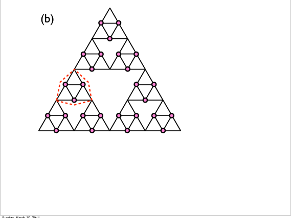
Figure 1: (Color online) Vertex covering for (a) a triangular lattice and (b) a Sierpinski gasket. In both cases, the optimal coverage (large dots) is imperfect (i.e., some edges possess double coverings). Yet, these solutions either are unique, as for the Sierpinski gasket, or possess a finite symmetry, such as the possible translations on the triangular lattice, both cases leading to a vanishing entropy density. For both lattices it is easily seen that the asymptotic coverage is $\frac{2}{3}$. In the case of the triangular lattice, the unit cell (dashed red box) contains two vertices completely and shares half of eight vertices with other cells, i.e., it has effectively $2+\frac{8}{2}=6$ vertices of which $1+\frac{6}{2}=4$ are covered. The unit cell in the Sierpinski gasket contains $3+\frac{3}{2}$ vertices of which the three fully contained ones must be covered.

This paper is organized as follows. In Sec. II we review the properties of the Hanoi networks. In Sec. III we briefly recount the relevant theory for a thermodynamic study of vertex cover in terms of a hard-core lattice gas. In Sec. IV, we develop the renormalization group treatment of the lattice gas, with most of the technical details deferred to the Appendix Appendix, and its application to the Hanoi networks HN3 and HN5. A detailed numerical study of the problem follows in Sec. V. We present our conclusions and an outlook for future work in Sec. VI.

II Geometry of the Hanoi Networks

Each of the Hanoi networks possesses a simple geometric backbone, a one-dimensional line of sites $0\leq n<N=2^{k}+1$ (Boettcher et al., 2008a; Boettcher and Goncalves, 2008). Most importantly, all sites are connected to their nearest neighbors, ensuring the existence of the $1d$-backbone. To generate the small-world hierarchy in these networks, consider parameterizing any integer $n$ (except for zero) uniquely in terms of two other integers $(i,j)$, $i\geq 1$, via

$$n = 2^{i-1}\left(2j+1\right),$$ (1)

where $i$ denotes the level in the hierarchy and $j$ labels consecutive sites within each hierarchy. For instance, $i=1$ refers to all odd integers, $i=2$ to all integers once divisible by 2 (i.e., 2, 6, 10,…), and so on. In these networks, aside from the backbone, each site is also connected with some of its neighbors within the hierarchy. For example, we obtain a 3-regular network HN3 (best done on a semi-infinite line) by connecting first the backbone, then 1 to 3, 5 to 7, 9 to 11, etc, for $i=1$, next 2 to 6, 10 to 14, etc, for $i=2$, and 4 to 12, 20 to 28, etc, for $i=3$, and so on, as depicted in Fig. 2. Previously (Boettcher et al., 2008a), it was found that the average chemical path between sites on HN3 scales as

$$d^{HN3}\sim\sqrt{l}$$ (2)

with the distance $l$ along the backbone.

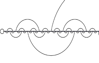
Figure 2: Depiction of the 3-regular network HN3 on a semi-infinite line. Note that HN3 is planar.

While HN3 is of a fixed, finite degree, there exist generalizations of HN3 that lead to new, revealing insights into small-world phenomena (Boettcher et al., 2008a; Boettcher and Goncalves, 2008; Boettcher et al., 2011). For instance, we can extend HN3 in the following manner to obtain a network of average degree 5, hence called HN5. In addition to the edges in HN3, in HN5 we also connect each site in level $i$ ($i\geq 2$, i.e., all even sites), to (higher-level) sites that are $2^{i-1}$ sites away in both directions. Note that Eq. (1) implies that the nearest neighbors of a site $i$ within its hierarchy are separated by a distance of $2\times 2^{i-1}$. The resulting network HN5 remains planar but now sites have a hierarchy-dependent degree, as shown in Fig. 3. To obtain the average degree, we observe that 1/2 of all sites have degree 3, 1/4 have degree 5, 1/8 have degree 7, and so on, leading to an exponentially falling degree distribution of ${\cal P}\left\{\alpha=2i+1\right\}\propto 2^{-i}$. Then, the total number of edges $L$ in a system of size $N=2^{k}+1$ as shown in Fig. 3 is

$$2L =2\left(2k+1\right)+ \sum_{i=1}^{k-1}\left(2i+1\right)2^{k-i}=5\times 2^{k}-4,$$ (3)

where the expression outside the sum refers to the special case of those three vertices at the highest levels, $k-1$ and $k$. Any other choice of boundary conditions may vary the offset in Eq. (3), but not the average degree, which is

$$\left\langle\alpha\right\rangle = \frac{2L}{N}\sim 5.$$ (4)

In HN5, the end-to-end distance is trivially 1 (see Fig. 3). Therefore, we define as the diameter the largest of the shortest paths possible between any two sites, which are typically odd-index sites farthest away from long-distance edges. For the $N=33$ site network depicted in Fig. 3, for instance, that diameter is 5, measured between sites 3 and 19 (starting with $n=0$ as the left-most site), although there are many other such pairs. It is easy to show recursively that this diameter grows as

$$d^{\rm HN5} = 2\left\lfloor k/2\right\rfloor+1\sim\log_{2}N.$$ (5)

Other variants of the Hanoi networks are conceivable. For instance, a non-planar version has been designed (Boettcher et al., 2009; Boettcher and Brunson, ), but that network happens to possess only a unique, alternating covering of $\frac{1}{2}$ and is not considered here.

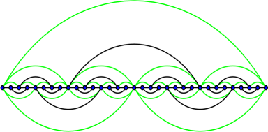
Figure 3: (Color online) Depiction of the planar network HN5, consisting of an HN3 core (black lines) with the addition of farther-reaching long-range edges (shaded lines). Note that sites on the lowest level of the hierarchy have degree 3, then degree 5, 7, etc, comprising a fraction of $1/2,$ $1/4$, $1/8$, etc., of all sites, which makes for an average degree of 5 in this network. (There is no distinction made between black and shaded lines in our studies here.)

III Vertex-Cover Problem as a Hard-Core Lattice Gas

Vertex cover is a well-known NP-hard combinatorial problem (Karp, 1972; Garey and Johnson, 1979; Ausiello et al., 1999) that consists of finding a minimal covering of the vertices of a network in such a way that each edge is covered at least once. Formally, for a graph $G=(V,E)$, with $V$ being the set of vertices and $E\subset V^{(2)}$ the set of edges, a vertex cover $V^{\prime}$ is a subset of $V$ with the property that for each (undirected) edge $\{i,\,j\}\in E$ either $i\in V^{\prime}$ or $j\in V^{\prime}$. A minimum vertex cover $V_{\min}$ is a vertex cover of minimum cardinality $|V_{\min}|$.

As shown in Ref. (Weigt and Hartmann, 2001), the vertex-cover problem can be formulated alternatively as a hard-core repulsive lattice gas problem. In this formulation, the uncovered vertices of the covering problems correspond to the actual gas particles. These particles have a hard-core repulsion such that they can not occupy neighboring lattice sites, i.e., they cannot simultaneously vie for the same edge. Interpreting these particles as the voids of the covering problem implies that no edge may be left uncovered on both ends. Accordingly, all properties of the minimum cover problem derive from the ground state of the lattice gas at its highest packing.

The grand canonical partition function for such a lattice gas is generically given by

$$\Xi\left(\mu\right) = \sum_{x_{0}=\{0,1\}}\ldots\sum_{x_{N}=\{0,1\}}\exp\left(\mu\sum_{i=1}^{N}x_{i}\right)\prod_{\langle i,j\rangle}\left(1-x_{i}x_{j}\right),$$ (6)

where the product extends over all edges of the graph and exerts the hard-core repulsive constraint. The chemical potential $\mu$ is provided to regulate the density as gas particles get packed into the system. Since maximal density of the gas implies minimal coverage of all edges, we are looking for the configurations in the limit $\mu\to\infty$ of the gas.

The quantities (Weigt and Hartmann, 2001) we seek are the thermodynamic limit ($N\to\infty$) of the packing fraction for the lattice gas,

$$\nu\left(\mu\right) = \frac{1}{N}\left\langle\sum_{i=1}^{N}x_{i}\right\rangle_{\mu}=\frac{1}{N}\frac{\partial}{\partial\mu}\ln\Xi\left(\mu\right),$$ (7)

and the entropy density of such configurations,

$$s\left(\nu\left(\mu\right)\right) = \frac{1}{N}\left(1-\mu\frac{\partial}{\partial\mu}\right)\ln\Xi\left(\mu\right).$$ (8)

It has also been shown in Ref. (Weigt and Hartmann, 2001) that one can extract the corresponding properties of the minimal vertex coverage from these in the $\mu\to\infty$ limit. For the coverage density, this corresponds simply to the void density of the gas,

$$c_{\rm min} = 1-\lim_{\mu\to\infty}\nu\left(\mu\right),$$ (9)

and the entropy density of optimal coverages is simply equal to that for the lattice gas:

$$s_{\rm VC}\left(c_{\rm min}\right) = s\left(\nu=1-c_{\rm min}\right).$$ (10)

Due to the hierarchical structure of the Hanoi networks, we will also introduce level-specific chemical potentials $\mu_{i}$, for example, to extract information about the coverage with respect to the level of the hierarchy (i.e., the range its small-world edge attains) that a vertex may reside in. The corresponding derivations are presented in the Appendix. Throughout, we will find it often convenient to express the chemical potentials as an activity variable,

$$m_{i} = e^{-\mu_{i}}\qquad\left(1\leq i\leq k\right),$$ (11)

such that $\mu_{i}\to\infty$ corresponds to the somewhat more tractable limit $m_{i}\to 0$.

IV RG for the Hard-Core Lattice Gas on Hanoi Networks

The renormalization group (RG) as applied to the lattice-gas problem developed here contains a few unfamiliar features. Thus, we have to elaborate to a significant extend on the procedure. Although ultimately the RG will heavily rely on procedures used for Ising spin models, initially we will have to rewrite the grand canonical partition function of the lattice gas in an appropriate form. To this end, the purpose of the first step of the RG (already eliminating half of all sites) is to generate the initial conditions for the subsequent canonical partition function analysis, in which the usual coupling variables depend in a complicated way on the chemical potential $\mu$ instead of a temperature, and the apparent “spin” variables are in fact Boolean, $x_{i}\in\left\{0,1\right\}$.

We have to rewrite the generic partition function in Eq. (6) for the special case of the Hanoi networks. To access more details of the solutions, we will take the opportunity to generalize to the case of a hierarchy-specific chemical potential $\mu_{i}$ for $1\leq i\leq k$, where $N=2^{k}+1$ is the size of the system. (For the RG, it is natural to consider the Hanoi network with an open boundary both at node $0$ and at node $2^{k}$; for a system with periodic boundaries on a loop, both of these nodes would become identical and $N=2^{k}$ would be the size of the system. Of course, either choice results in identical thermodynamic averages.)

First, we rewrite the hard-core repulsive factor in Eq. (6) as separate products, one for the long-range edges and the other for the backbone edges,

$$\prod_{\langle i,j\rangle}\left(1-x_{i}x_{j}\right) = \left[\prod_{i=1}^{{\cal K}}\prod_{n=1}^{2^{k+1-i}}\left(1-x_{2^{i-1}\left(n-1\right)}x_{2^{i-1}n}\right)\right]\left[\prod_{i=1}^{k-1}\prod_{l=1}^{2^{k-i-1}}\left(1-x_{2^{i-1}\left(4l-3\right)}x_{2^{i-1}\left(4l-1\right)}\right)\right].$$ (12)

The case ${\cal K}=1$ corresponds to HN3, with a simple, one-dimensional line of edges connecting all sites in the backbone sequentially. In turn, for HN5 we set ${\cal K}=k$, with each $i>1$ referring to the layers of those edges that connect along the backbone only every second site, every fourth site, every eight site, etc., as shown in Fig. 3. Note that in Eq. (12) we have used the decomposition of the sites in the network implied by the renumbering in Eq. (1).

By the same token, we re-order the summation in Eq. (6) as

$$\sum_{x_{0}}e^{\mu_{i(0)}x_{0}}\ldots\sum_{x_{N}}e^{\mu_{i(N)}x_{N}} = \sum_{x_{0}}m_{i(0)}^{-x_{0}}\ldots\sum_{x_{N}}m_{i(N)}^{-x_{N}},$$

$$= \sum_{x_{0},x_{2^{k-1}},x_{2^{k}}}m_{k}^{-x_{0}-x_{2^{k-1}}-x_{2^{k}}}\left[\prod_{i=1}^{k-1}\prod_{l=1}^{2^{k-i-1}}\sum_{x_{2^{i-1}\left(4l-3\right)}}\sum_{x_{2^{i-1}\left(4l-1\right)}}m_{i}^{-x_{2^{i-1}\left(4l-3\right)}-x_{2^{i-1}\left(4l-1\right)}}\right],$$

where we have simplified the notation on the sums to mean $\sum_{x}\hat{=}\sum_{x\in\left\{0,1\right\}}$. Of course, Eq. (IV) has to be understood in an operator sense, i.e., the summations extend to all site-variables that match the indicated index. Here, we have also allowed for a site-specific chemical potential. It is our goal to extract local packing information, not for each site, but for all vertices within a specific hierarchy, where $i(n)$ refers to the chemical potential in the $i$-th level that the vertex $n$ is associated with according to Eq. (1). Naturally, the sites at the highest level $k$ of the hierarchy ($x_{0},x_{2^{k-1}},x_{2^{k}}$) require special consideration.

In this parametrization of the indices, the products in Eq. (IV) can be combined with those of the second factor in Eq. (12). Both refer to the small-world edges in all levels of the hierarchy and are naturally expressed in a hierarchy-conform manner. Hence, we find for the grand-canonical partition function defined in Eq. (6) on a Hanoi network with $k$ levels in the hierarchy:

$$\Xi^{(k)}_{{\cal K}}\left(m_{1,}\dots,m_{k}\right) = \sum_{x_{0},x_{2^{k-1}},x_{2^{k}}}m_{k}^{-x_{0}-x_{2^{k-1}}-x_{2^{k}}}\,{\cal S}_{{\cal K}}\left(m_{2,}\dots,m_{k-1}\right)\,\prod_{j=1}^{2^{k-2}}\Theta\left(m_{1},x_{2\left(2j-2\right)},x_{2\left(2j-1\right)},x_{2\left(2j\right)}\right),$$ (14)

where we have defined the operator for the weighted summation on HN3 and HN5, respectively,

$${\cal S}_{\rm HN3} \equiv \prod_{i=2}^{k-1}\prod_{l=1}^{2^{k-i-1}}\sum_{x_{2^{i-1}\left(4l-3\right)}}\sum_{x_{2^{i-1}\left(4l-1\right)}}m_{i}^{-x_{2^{i-1}\left(4l-3\right)}-x_{2^{i-1}\left(4l-1\right)}}\left(1-x_{2^{i-1}\left(4l-3\right)}x_{2^{i-1}\left(4l-1\right)}\right),$$

$${\cal S}_{\rm HN5} \equiv \prod_{i=2}^{k-1}\prod_{l=1}^{2^{k-i-1}}\sum_{x_{2^{i-1}\left(4l-3\right)}}\sum_{x_{2^{i-1}\left(4l-1\right)}}m_{i}^{-x_{2^{i-1}\left(4l-3\right)}-x_{2^{i-1}\left(4l-1\right)}}\left(1-x_{2^{i-1}\left(4l-3\right)}x_{2^{i-1}\left(4l-1\right)}\right)$$

$$\times\left(1-x_{2^{i-1}\left(4l-4\right)}x_{2^{i-1}\left(4l-3\right)}\right)\left(1-x_{2^{i-1}\left(4l-3\right)}x_{2^{i-1}\left(4l-2\right)}\right)\left(1-x_{2^{i-1}\left(4l-2\right)}x_{2^{i-1}\left(4l-1\right)}\right)\left(1-x_{2^{i-1}\left(4l-1\right)}x_{2^{i-1}\left(4l\right)}\right).$$

Note that these operators only sum over all even-indexed variables (i.e., $i\geq 2$). To obtain a renormalizable form for the partition function it is necessary to trace over the lowest level $i=1$ of the hierarchy, i.e., to eliminate all odd-index variables. For both, HN3 and HN5, this results in an identical structure, defined as

$$\Theta\left(\mu_{1},x_{2\left(2j-2\right)},x_{2\left(2j-1\right)},x_{2\left(2j\right)}\right) = \sum_{x_{4j-3}}\sum_{x_{4j-1}}m_{1}^{-x_{4l-3}-x_{4l-1}}\left(1-x_{4j-3}x_{4j-1}\right)$$

$$\quad\left(1-x_{4j-4}x_{4j-3}\right)\left(1-x_{4j-3}x_{4j-2}\right)\left(1-x_{4j-2}x_{4j-1}\right)\left(1-x_{4j-1}x_{4j}\right),$$

$$= 1+e^{\mu_{1}}\left(1-x_{2\left(2j-1\right)}\right)\left(2-x_{2\left(2j-2\right)}-x_{2\left(2j\right)}\right).$$

In Appendix A, we show how to recast $\Theta$ in an Ising-like form with a sufficient number of renormalizable parameters. We can simplify the grand partition function in Eq. (14) further by combining the products and writing

$$\Xi^{(k)}\left(m_{1},\ldots,m_{k}\right) = \sum_{x_{0},x_{2^{k-1}},x_{2^{k}}}m_{k}^{-x_{0}-x_{2^{k-1}}-x_{2^{k}}}\left[\prod_{i=2}^{k-2}\prod_{l=1}^{2^{k-i-2}}\sum_{x_{2^{i}\left(4l-3\right)}}\sum_{x_{2^{i}\left(4l-1\right)}}\right]\prod_{l=1}^{2^{k-3}}\zeta_{1}^{l}\left(x_{4\left(2l-2\right)},x_{4\left(2l-1\right)},x_{4\left(2l\right)}\right),$$ (16)

where the explicit expression for $\zeta_{1}^{l}$ is also derived in Appendix A for both, HN3 and HN5, which allows us to drop the subscript label. In either case, the RG recursion equations now result from imposing the recursive relation between hierarchies,

$$\zeta_{i+1}^{l}\left(x_{2^{i+1}\left(2l-2\right)},x_{2^{i+1}\left(2l-1\right)},x_{2^{i+1}\left(2l\right)}\right)$$

$$= \sum_{x_{2^{i}\left(4l-3\right)}}\sum_{x_{2^{i}\left(4l-1\right)}}\zeta_{i}^{2l-1}\left(x_{2^{i}\left(4l-4\right)},x_{2^{i}\left(4l-3\right)},x_{2^{i}\left(4l-2\right)}\right)\zeta_{i}^{2l}\left(x_{2^{i}\left(4l-2\right)},x_{2^{i}\left(4l-1\right)},x_{2^{i}\left(4l\right)}\right),$$

which are derived in Appendix A. There, Figs. 15 and 16 also provide a graphical representation of Eq. (IV).

IV.1 Analysis of the RG Recursions

We find that the RG recursions that follow from the previous discussion, which are given explicitly in Eqs. (52) for HN3 and in Eqs. (54) for HN5 for the hard-core lattice gas model, have only two trivial fixed points. There is a stable low-density fixed point for all $\mu<\infty$, i.e., $m>0$, and an unstable fixed point at full-packing for $\mu=\infty$, i.e., $m=0$. Note that in this part of the analysis we are concerned with global properties, and thus, ignore differences between the hierarchical level by setting $m_{i}\equiv m$ throughout.

IV.1.1 Analysis for HN3

The limit $m\to 0$ of the recursions in Eqs. (52) for initial conditions given in Eqs. (50) is difficult to handle. Except for $\kappa_{1}$, all other parameters are either diverging or vanishing in Eqs. (18) for that limit. To achieve a clearer picture, we evolve the recursions once and obtain

$$\eta_{2}\sim\frac{24}{5},\quad\gamma_{2}\sim\frac{8}{3},\quad C_{2}\sim\frac{m^{2}}{8}, \kappa_{2}\sim\frac{15}{8},\quad\lambda_{2}\sim\frac{25}{24},\quad\Delta_{2}\sim\frac{4}{25m}.$$ (18)

In fact, further revolutions in the recursions seems to preserve this picture: $C_{i}$ scales with a rapidly growing power of $m$, while all other parameters and $\bar{\Delta}_{i}=m\Delta_{i}$ become finite for $m=0$ at any order $i$. Thus, we replace $\Delta$ with $\bar{\Delta}$ and subsequently set $m\to 0$ in Eqs. (52) yielding

$$C_{i+1}\sim\frac{m\gamma_{i}C_{i}^{2}}{2}, \gamma_{i+1}\sim\gamma_{i}\eta_{i}\kappa_{i},\qquad\eta_{i+1}\sim\frac{4\kappa_{i}}{\left(1+\kappa_{i}\right)^{2}},$$

$$\kappa_{i+1}\sim\lambda_{i}\frac{\left(1+\kappa_{i}\right)}{\kappa_{i}}, \lambda_{i+1}\sim\frac{\left(1+\kappa_{i}\right)^{2}}{4\kappa_{i}},\qquad\bar{\Delta}_{i+1}\sim\frac{2\kappa_{i}^{2}\bar{\Delta}_{i}}{\left(2+\gamma_{i}\kappa_{i}^{2}\bar{\Delta}_{i}\right)\left(1+\kappa_{i}\right)^{2}}.$$ (19)

At its core, the two recursions for $\kappa$ and $\lambda$ have become independent of all the others. The $m=0$ fixed-point itself is then dominated solely by the stationary solution of their recursions in Eqs. (19),

$$\kappa^{*}=\frac{1}{2^{\frac{2}{3}}-1}, \lambda^{*}=\frac{1}{2^{\frac{2}{3}}\left(2^{\frac{2}{3}}-1\right)}.$$ (20)

Therefore, one finds a constant solution for $\eta^{*}=4\kappa^{*}/\left(1+\kappa^{*}\right)^{2}=1/\lambda^{*}$ and the recursion $\gamma_{i+1}\sim\gamma_{i}\left(\kappa^{*}/\lambda^{*}\right)$ with the solution $\gamma_{i}\sim\gamma_{0}2^{\frac{2i}{3}}$ which diverges for large $i$. The situation for $\bar{\Delta}_{i}$ is more subtle. Numerics clearly indicates its decay, but this could occur consistently in two ways. First, if it were to decay such that $\gamma_{i}\bar{\Delta}_{i}$ still increases, then Eq. (19) suggests $\bar{\Delta}_{i+1}\propto 1/\gamma_{i}$, but that would render $\gamma_{i}\bar{\Delta}_{i}$ constant, which is a contradiction. Alternatively, if both $\bar{\Delta}_{i}$ and $\gamma_{i}\bar{\Delta}_{i}$ decay, then $\bar{\Delta}_{i+1}\sim\bar{\Delta}_{i}\left[\kappa^{*}/\left(1+\kappa^{*}\right)\right]^{2}$, yielding $\bar{\Delta}_{i}\sim 2^{-\frac{4i}{3}}$ in a consistent manner. Numerical studies verify that the latter solution is indeed realized.

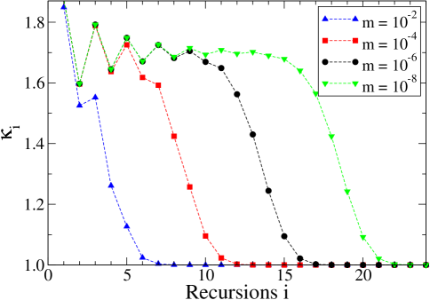
Figure 4: (Color online) Plot of the value of $\kappa_{i}$ after the $i$-th RG-step for $m=10^{-2},10^{-4},10^{-6},$ and $10^{-8}$ (left to right). At a length scale $\xi\left(m\right)=2^{i}$ with $i=-\frac{3}{4}\log_{2}m$, the behavior of $\kappa_{i}$ crosses over from the value at the unstable $m=0$ fixed point, $\kappa^{*}=1/\left(2^{2/3}-1\right)\approx 1.70$, to the stable $m=1$ ($\mu=0$) fixed point at which $\kappa^{*}=1$.

From the terms dropped in the $m\to 0$ limit, we can extract a cross-over scale as follows: Achieving the limit $m\to 0$ implies that the widely occurring term $m\gamma_{i}$ in Eqs. (52) is considered small enough to be discarded with respect to terms of order unity. Hence, by identifying $\xi=\sqrt{2^{i(m)}}$ as the correlation length within the small-world metric supplied by Eq. (2), using $\gamma_{i(m)}\sim 1/m$ yields $2^{i(m)}\sim m^{-\frac{3}{2}}$ or

$$\xi \sim e^{\frac{3}{4}\mu}$$ (21)

as the diverging length below which the systems orders for an correspondingly diverging chemical potential, $\mu\to\infty$. Indeed, for $m=10^{-4}$, for example, we find numerically that the solution veers off the unstable fixed point just below the $i=10$th iteration; Fig. 4 demonstrates the correctness of Eq. (21) for any small $m$.

IV.1.2 Analysis for HN5

The analysis for HN5 is surprisingly subtle. Although the preceding fixed-point analysis for HN3 required the singular limit $m\to 0$ as part of the consideration, after the appropriate rescaling of the parameters with $m$, the subsequent approach proceeds in a familiar fashion. HN5 obscures this approach with an additional layer of complexity, resulting from strong alternating effects order-by-order in the RG, as the numerics reveals. Of course, the initial conditions here are identical to those for HN3 in Eqs. (50), with the same pathologies in the $m\to 0$ limit. However, whereas those problems were essentially resolved for HN3 after one RG-step and rescaling, see Eqs. (18), here we find

$$C_{2}\sim\frac{m^{2}}{2},\quad\gamma_{2}\sim 2,\quad\eta_{2}\sim\frac{8}{9},\quad\kappa_{2}\sim\frac{3}{8m},\quad\lambda_{2}\sim\frac{9}{8},\quad\Delta_{2}\sim\frac{8}{9},$$ (22)

and

$$C_{3}\sim\frac{m^{5}}{16},\quad\gamma_{3}\sim\frac{16}{9m},\quad\eta_{3}\sim 16m,\quad\kappa_{3}\sim\frac{9}{16},\quad\lambda_{3}\sim\frac{1}{16m},\quad\Delta_{3}\sim 16m,$$ (23)

etc. This alternation between regular and singular behaviors of each of the parameters persists thereafter. Leaving the recursion for $C_{i}$ aside for now, we notice that for even indices, $\gamma_{2n}$, $\eta_{2n}$, $m\kappa_{2n}$, $\lambda_{2n}$, and $\Delta_{2n}$ remain finite for $m\to 0$, but for odd indices, this is true for $m\gamma_{2n-1}$, $\eta_{2n-1}/m$, $\kappa_{2n-1}$, $m\lambda_{2n-1}$, and $\Delta_{2n-1}/m$. Defining $\bar{\gamma}_{2n-1}=m\gamma_{2n-1}$, $\bar{\eta}_{2n-1}=\eta_{2n-1}/m$, $\bar{\kappa}_{2n}=m\kappa_{2n}$, $\bar{\lambda}_{2n-1}=m\lambda_{2n-1}$, and $\bar{\Delta}_{2n-1}=\Delta_{2n-1}/m$, it is useful to rewrite the recursions in Eqs. (54) separately for even and odd indices. In fact, the limit $m\to 0$ on its explicit appearance can now be taken to get

$$\gamma_{2n}=\bar{\eta}_{2n-1}\left(2+\bar{\gamma}_{2n-1}\right), \bar{\gamma}_{2n-1}=\eta_{2\left(n-1\right)}\left(2+m\gamma_{2\left(n-1\right)}\right)\sim 2\eta_{2\left(n-1\right)},$$

$$\eta_{2n}=\bar{\gamma}_{2n-1}\frac{2+\bar{\gamma}_{2n-1}}{\left(1+\bar{\gamma}_{2n-1}\right)^{2}}, \bar{\eta}_{2n-1}=\gamma_{2\left(n-1\right)}\frac{2+m\gamma_{2\left(n-1\right)}}{\left(1+m\gamma_{2\left(n-1\right)}\right)^{2}}\sim 2\gamma_{2\left(n-1\right)},$$

$$\bar{\kappa}_{2n}=\bar{\lambda}_{2n-1}\frac{\left(1+\bar{\gamma}_{2n-1}\right)^{2}}{2+\bar{\gamma}_{2n-1}}, \kappa_{2n-1}=\lambda_{2\left(n-1\right)}\frac{1+m\gamma_{2\left(n-1\right)}}{2+m\gamma_{2\left(n-1\right)}}\sim\frac{1}{2}\lambda_{2\left(n-1\right)},$$ (24)

$$\lambda_{2n}=\frac{\left(1+\bar{\gamma}_{2n-1}\right)^{2}}{\bar{\gamma}_{2n-1}\left(2+\bar{\gamma}_{2n-1}\right)}, \bar{\lambda}_{2n-1}=\frac{1+m\gamma_{2\left(n-1\right)}}{\gamma_{2\left(n-1\right)}\left(2+m\gamma_{2\left(n-1\right)}\right)}\sim\frac{1}{2\gamma_{2\left(n-1\right)}},$$

$$\Delta_{2n}=\bar{\gamma}_{2n-1}\frac{2+\bar{\gamma}_{2n-1}}{\left(1+\bar{\gamma}_{2n-1}\right)^{2}}, \bar{\Delta}_{2n-1}=\gamma_{2\left(n-1\right)}\frac{2+m\gamma_{2\left(n-1\right)}}{\left(1+m\gamma_{2\left(n-1\right)}\right)^{2}}\sim 2\gamma_{2\left(n-1\right)}.$$

Note that for the limit $m\to 0$ we only assumed that $m\gamma_{2\left(n-1\right)}\ll 1$ for $n\to\infty$ on the right-hand set of these relations, which provides a correlation length from the cross-over $n_{\rm co}=n\left(m\right)$ at $\gamma_{2n_{\rm co}}\sim 1/m$. Eliminating all odd-index quantities from the equations yields

$$\gamma_{2n}=4\gamma_{2\left(n-1\right)}\left(1+\eta_{2\left(n-1\right)}\right), \eta_{2n}=4\eta_{2\left(n-1\right)}\frac{1+\eta_{2\left(n-1\right)}}{\left(1+2\eta_{2\left(n-1\right)}\right)^{2}},$$ (25)

$$\bar{\kappa}_{2n}=\frac{1+2\eta_{2\left(n-1\right)}}{4\gamma_{2\left(n-1\right)}\left(1+\eta_{2\left(n-1\right)}\right)}, \lambda_{2n}=\frac{\left(1+2\eta_{2\left(n-1\right)}\right)^{2}}{4\eta_{2\left(n-1\right)}\left(1+\eta_{2\left(n-1\right)}\right)},\qquad\Delta_{2n}=4\eta_{2\left(n-1\right)}\frac{1+\eta_{2\left(n-1\right)}}{\left(1+2\eta_{2\left(n-1\right)}\right)^{2}}.$$

These interlacing recursions now have a simple fixed point, which derives from the only non-trivial solution of the self-contained $\eta$-equation:

$$\eta^{*}=\frac{\sqrt{3}}{2}.$$ (26)

This implies the equally stationary value

$$\Delta^{*}=\frac{1}{\lambda^{*}}=\frac{4\eta^{*}\left(1+\eta^{*}\right)}{\left(1+2\eta^{*}\right)}=\frac{3+\sqrt{3}}{2},$$ (27)

but we also find the asymptotically scaling

$$\gamma_{2n}\sim\gamma_{0}\left[2\left(2+\sqrt{3}\right)\right]^{n}\propto\frac{1}{\bar{\kappa}_{2n}}.$$ (28)

This provides the correlation length estimate

$$\xi=2^{n_{\rm co}}\sim\exp\left\{\frac{\mu}{\log_{2}\left[2\left(2+\sqrt{3}\right)\right]}\right\}.$$ (29)

IV.2 Packing Fraction and Entropy

To understand the most pertinent features of the problem, such as the optimal packing (or coverage) and its entropy, we have to consider the asymptotic behavior of the renormalization group parameter $C_{i}$, related to the growth of the overall energy-scale, in Eq. (19) for the initial condition in Eq. (18). Clearly, the partition function at any finite system size is a polynomial in $e^{\mu}$, i.e., in powers of $m^{-1}$. Both of these quantities, packing fraction and entropy, derive from the most divergent power in $m$ to be found in $\Xi$. To wit, we can write for $m\to 0$ with $N=2^{k}+1$,

$$\Xi^{(k)} \sim \left(\sigma m^{-\alpha}\right)^{N}\left[1+am+bm^{2}+\ldots\right].$$ (30)

Then, it is $\partial_{\mu}\ln\Xi=-m\partial_{m}\ln\Xi\sim N\alpha$, and we find from Eqs. (7 and 8),

$$\nu = \alpha,$$

$$s = \ln\sigma,$$

for $N\to\infty$ at $m=0$.

Equation (16) provides the grand canonical partition function $\Xi^{(k)}$ for $2^{k}+1$ site-occupation variables in terms of an Ising-like canonical partition function ${\cal Z}^{(k-1)}$ for only $2^{k-1}+1$ (Boolean) spin variables. While $\Xi^{(k)}$ depends only on the hierarchical chemical potentials $m_{i}$, ostensibly ${\cal Z}^{(k-1)}$ depends on a tuple $\vec{A}_{1}$ of renormalizable couplings, see Eq. (55), in addition to any explicit dependence on $m_{i}$. Of course, the couplings themselves are merely a function of the chemical potentials, $\vec{A}_{1}=\vec{A}_{1}\left(m_{1}\right)$, through the RG initial conditions in Eq. (50). Step by step in the RG, the couplings transform according to Eq. (56) each time the system size halves, whereas the partition function stays invariant. Hence, we can expand on Eq. (16) and write

$$\Xi^{(k)}\left(m_{1},\ldots,m_{k}\right) = {\cal Z}^{(k-1)}\left(\vec{A}_{1}\left(m_{1}\right),m_{2},\ldots,m_{k}\right),$$

$$= {\cal Z}^{(k-2)}\left(\vec{A}_{2}\left(m_{1},m_{2}\right),m_{3},\ldots,m_{k}\right),$$

$$\vdots$$

$$= {\cal Z}^{(1)}\left(\vec{A}_{k-1}\left(m_{1},\ldots,m_{k-1}\right),m_{k}\right),$$

where ${\cal Z}^{(1)}$ is simply a rudimentary Hanoi network consisting of just three vertices.

IV.2.1 Results for HN3

Specializing this discussion for HN3, we find for the rudimentary partition function ${\cal Z}^{(1)}$ in this case

$${\cal Z}^{(1)} = C_{k-1}^{-1}\sum_{x_{0}}\sum_{x_{2^{k-1}}}\sum_{x_{2^{k}}}m_{k}^{-\left(x_{0}+x_{2^{k-1}}+x_{2^{k}}\right)}\gamma_{k-1}^{-\frac{1}{2}\left[\left(x_{0}+x_{2^{k-1}}\right)+\left(x_{2^{k-1}}+x_{2^{k}}\right)\right]}$$ (32)

$$\qquad\eta_{k-1}^{-\frac{1}{2}\left(x_{0}+x_{2^{k}}\right)}\kappa_{k-1}^{-\left(x_{0}x_{2^{k-1}}+x_{2^{k-1}}x_{2^{k}}\right)}\lambda_{k-1}^{-x_{0}x_{2^{k}}}\Delta_{k-1}^{-x_{0}x_{2^{k-1}}x_{2^{k}}}.$$

For a uniform chemical potential, $m_{i}\equiv m$ for all $i$, one finds that for $m\to 0$ the partition function is dominated overwhelmingly by the renormalized value of $C_{i}$, i.e.

$$\ln\Xi^{(k)}\left(\mu\right) = \ln{\cal Z}^{(1)}(\vec{A}_{k-1}\left(m\right),m)\sim-\ln C_{k-1}.$$ (33)

Rewriting the recursion for $C_{i}$ in Eq. (19) in this form yields

$$\ln C_{i+1} = 2\ln C_{i}+\ln\left(\frac{m\gamma_{i}}{2}\right)\sim 2\ln C_{i}+\frac{2i}{3}\ln 2+\ln\left(\frac{m\gamma_{0}}{2}\right),$$ (34)

which is easily summed up to give

$$\ln C_{k-1} = 2^{k-3}\left[\ln C_{2}+\ln\left(2m\gamma_{0}\right)\right].$$ (35)

With $C_{2}\sim m^{2}$, as listed in Eq. (18), we get

$$\frac{1}{2^{k}}\ln\Xi^{(k)} \sim -\frac{1}{2^{k}}\ln C_{k-1}\sim-\frac{3}{8}\ln\left(m\right)-\frac{1}{8}\ln\left(4\gamma_{0}\right),$$ (36)

and comparison with Eq. (30) produces an exact prediction for the maximal packing fraction of the lattice gas,

$$\nu\left(\mu\to\infty\right) = \frac{3}{8},$$ (37)

i.e., for the minimal fraction of vertices needing cover in HN3, it is

$$c_{\rm min} = \frac{5}{8}.$$ (38)

Note that the $m$-dependence of $C_{2}$ and of the recursion for $C_{i}$ in Eqs. (19) are crucial for this result, whereas $\gamma_{i}$ is independent of $m$ and, hence, becomes irrelevant here. Unfortunately, the entropy density in turn depends not only on the asymptotic form for $\gamma_{i}$ but on the non-trivial integration constant $\gamma_{0}$, which can not be determined from the asymptotic behavior of the RG flow; it is a global property of that flow and could depend on all its details. However, the result suggest that, at least for HN3, unlike for those lattices in Fig. 1, the entropy density does not vanish but attains a non-trivial value. In fact, using the recursions in Eqs. (52) for arbitrary $m$ and taking the $m\to 0$ limit only in the end, we can exactly determine the constant $\sigma$ defined in Eq. (30) for the first few values of $k$ (see Tab. 1). Finite-size extrapolation from the numerical evolution of the RG flow up to $k=25$ levels (i.e., system size $N=2^{25}$) for a finite but small value of $m=10^{-40}$ predicts that $s_{\rm VC}(c_{\rm min})=0.160426(1)$. (Any variation of $m$ over 10 decades does not affect the extrapolation at this accuracy.) For smaller system sizes we plot the packing fraction and the entropy density for the entire range of the chemical potential in Fig. 5. In Appendix, we describe how to evaluate derivatives of the partition function, such as those leading to $\nu$ and $s$, within the RG-scheme. There we also develop a method to probe the packing fraction for each level of the hierarchy; those results are plotted in Fig. 6.

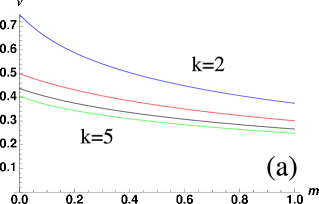
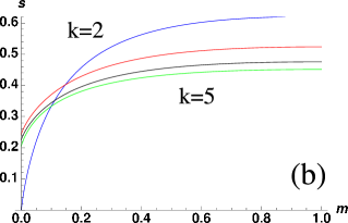
Figure 5: (Color online) Plot of (a) the packing fraction $\nu_{\rm VC}$ and (b) its entropy density $s_{\rm VC}$ for the lattice-gas problem on HN3 for the first few system sizes $N=2^{k}+1$ with $k=2,\ldots,5$ (top to bottom at $m=1$) as a function of $m$.

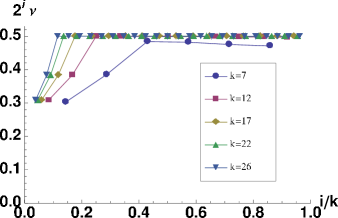
Figure 6: Plot of the relative packing per level $2^{i}\nu_{i}$ on HN3 for various system sizes $N=2^{k}+1$ with $k=7,12,17,22$, and 26, plotted also on a relative level-scale $i/k$ at $m\to 0$. Asymptotically, in large systems, all vertices in higher levels $i$ appear to be just 50% packed (or covered), which is minimally necessary to cover the one small-world edge connecting such vertices. (Of course, each level contains half as many vertices as any preceding level and thus contributes ever less to the overall coverage.) This packing may well be random as such vertices are far separated between the higher levels. A significantly lower packing (higher coverage) is attained only at an ever small fraction of the lowest levels to account for the overall packing fraction of $\frac{3}{8}$ (coverage $\frac{5}{8}$).

Table 1: Listing of the first few values of $\sigma$ and $s_{\rm VC}$ defined in Eqs. (30) and (10) for HN3 of size $N=2^{k}+1$. The sequence for the total number of optimal configurations, $\sigma^{N}$, soon develops non-trivial prime factors. The entropy density for the coverage $s_{\rm VC}$ only converges slowly to its numerical limit.

$k$	$\sigma^{N}\qquad$	$s_{\rm VC}=\ln\sigma$
2	1	0
3	7	0.243239
4	37	0.225682
5	718	0.205515
6	193284	0.190186
7	8651040480	0.178757
8	11491993035377280000	0.171438
$\vdots$	$\vdots$	$\vdots$
$\infty$		0.160426(1)

In the Appendix, we derive a partial set of recursions to approximate the number of solutions given in Tab. 1. Our failure to obtain a closed set of such equations (and an asymptotic prediction) indicates the non-trivial origin of the entropy density. Here, we just plot the exact solutions for $k=3$ and 4 for illustration in Figs. 7 and 8. As the numerical results in Sec. V indicate, the optimal packing of the lattice gas at any finite size $N=2^{k}+1$ contains for any $k\geq 3$ exactly $3\times 2^{k-3}+1$ particles.

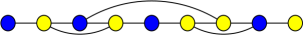
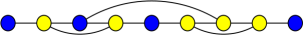
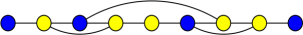
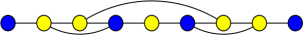
Figure 7: Depiction of perfect coverings on HN3 for $k=3$. Of all seven solutions, we omitted the three obtained by reflection from these. Light-colored sites belong to the vertex cover, dark-colored sites mark particles with hard-core repulsion that prevents nearest-neighbor occupation.

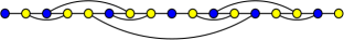
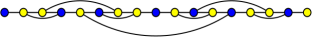
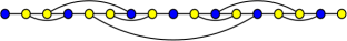
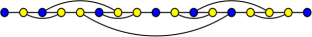
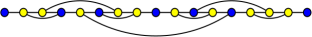
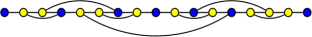
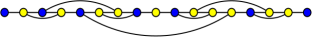
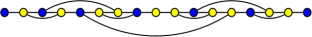
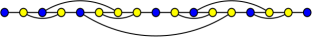
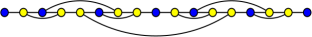
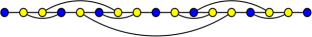
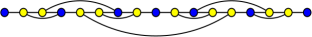
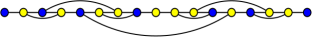
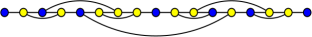
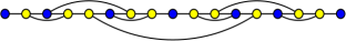
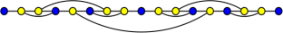
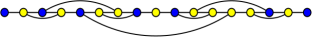
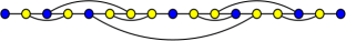
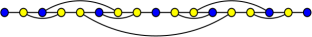
Figure 8: Depiction of perfect coverings on HN3 for $k=4$. Of all 37 solutions, we omitted the 17 obtained by reflection from these. Light-colored sites belong to the vertex cover, dark-colored sites mark particles with hard-core repulsion that prevents nearest-neighbor occupation.

IV.2.2 Results for HN5

For HN5, we find that the rudimentary partition function ${\cal Z}^{(1)}$ is like that for HN3 in Eq. (IV.2.2), except for additional repulsive terms:

$${\cal Z}^{(1)} = C_{k-1}^{-1}\sum_{x_{0}}\sum_{x_{2^{k-1}}}\sum_{x_{2^{k}}}m_{k}^{-\left(x_{0}+x_{2^{k-1}}+x_{2^{k}}\right)}\gamma_{k-1}^{-\frac{1}{2}\left[\left(x_{0}+x_{2^{k-1}}\right)+\left(x_{2^{k-1}}+x_{2^{k}}\right)\right]}$$

$$\qquad\eta_{k-1}^{-\frac{1}{2}\left(x_{0}+x_{2^{k}}\right)}\kappa_{k-1}^{-\left(x_{0}x_{2^{k-1}}+x_{2^{k-1}}x_{2^{k}}\right)}\lambda_{k-1}^{-x_{0}x_{2^{k}}}\Delta_{k-1}^{-x_{0}x_{2^{k-1}}x_{2^{k}}}$$

$$\qquad\left(1-x_{0}x_{2^{k-1}}\right)\left(1-x_{2^{k-1}}x_{2^{k}}\right)\left(1-x_{0}x_{2^{k}}\right).$$

Hence, Eq. (33) again applies, putting the focus on the analysis of the recursion for $C_{i}$, which in its even and odd versions read

$$C_{2n}=\frac{\bar{\gamma}_{2n-1}}{2+\bar{\gamma}_{2n-1}}C_{2n-1}^{2}, C_{2n-1}=\frac{m\gamma_{2\left(n-1\right)}}{2+m\gamma_{2\left(n-1\right)}}C_{2\left(n-1\right)}^{2}.$$ (40)

With the results from Sec. IV.1.2 at hand, when put together in the limit $m\to 0$, both recursions combine into

$$C_{2n} \sim mC_{2\left(n-1\right)}^{4}\left\{A\gamma_{2n}\right\}.$$ (41)

The factor $A\gamma_{2n}$, even though it grows exponentially with $n$, can be ignored because it does not depend on $m$. It is again easy to sum up the logarithm of this equation (for odd values of $k$, in this case) to get

$$\frac{1}{2^{k}}\ln C_{k-1} \sim \frac{1}{8}\ln C_{2}+\frac{1}{12}\ln m\sim\frac{1}{3}\ln m,$$ (42)

with $C_{2}\sim m^{2}$ from Eqs. (22). As for Eq. (36), for the maximal packing fraction of hard-core gas particles, this implies

$$\nu\left(\mu\to\infty\right) = \frac{1}{3},$$ (43)

i.e., for the minimal fraction of vertices needing cover in HN5, it is

$$c_{\rm min} = \frac{2}{3}.$$ (44)

In parallel to Sec. IV.1.1, we can obtain only the constant $\sigma$ defined in Eq. (30) for the first few values of $k$ (see Tab. 2). By the same procedure as for HN3 above, we predict here that $s_{\rm VC}(c_{\rm min})=0.11983(1)$. For smaller system sizes we plot the packing fraction and the entropy density for the entire range of the chemical potential in Fig. 9. Figure 10 illustrates the strong alternating behavior between successive levels, here in form of their relative packing fractions.

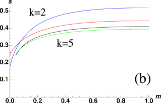
Figure 9: Plot of the packing fraction $\nu_{\rm VC}$ (left) and its entropy density $s_{\rm VC}$ for the lattice-gas problem on HN5 for the first few system sizes $N=2^{k}+1$ with $k=2,\ldots,5$ (with alternating behavior) as a function of $m$. Each entropy drops noticeably in the limit $m\to 0$.

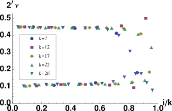
Figure 10: Plot of the relative packing per level $2^{i}\nu_{i}$ on HN5 for various system sizes $N=2^{k}+1$ with $k=7,12,17,22$, and 26, plotted also on a relative level-scale $i/k$ at $m\to 0$. In an alternating fashion levels attain an interlaced higher or lower relative packing (lower or higher coverage), which varies very little between the levels and seems to converge to nontrivial values. Notice that the apparent closing of the gap at the highest levels results from the numerical evaluation of the RG recursions at very small but still finite chemical activity (here, $m=10^{-9}$) .

Table 2: Listing of the first few values of $\sigma$ and $s_{\rm VC}$ defined in Eqs. (30) and (10) for HN5 of size $N=2^{k}+1$. The sequence for $\sigma^{N}$ soon develops non-trivial prime factors. The entropy density for the coverage $s_{\rm VC}$ alternates and only converges slowly to its numerically determined limit.

$k$	$\sigma^{N}\qquad$	$s_{\rm VC}=\ln\sigma$
2	2	0.173287
3	7	0.243239
4	6	0.111985
5	159	0.220479
6	1350	0.112623
7	21268575	0.131818
$\vdots$	$\vdots$	$\vdots$
$\infty$		0.11983(1)

V Monte Carlo Simulations

We performed Monte Carlo simulations of the lattice gas by using the grand canonical ensemble in Eq. (6). To achieve a fast convergence of the Markov chains, we used the Metropolis-Coupled Markov-Chain Monte Carlo (MCMCMC) approach (Geyer, 1991), also termed later Parallel Tempering (Hukushima and Nemoto, 1996) in the physics community. The idea of (MCMCMC) is to perform Monte Carlo simulations for $n$ independent replicas studied at different values of the chemical potential $\mu=\mu_{1},\ldots,\mu_{n}$ with $\mu_{1}=0<\mu_{2}<\ldots<\mu_{n}$. One allows that the replicas are exchanged via two-replica Metropolis steps, such that an overall detailed balance is achieved. Details of the Monte Carlo moves have been given in previous works, e.g. Ref. (Barthel and Hartmann, 2004). The parameters for the simulations performed for this work are shown in Tab. 3.

$N$	$n$	$\mu_{\max}$	$t_{{\rm MCS}}$
17	5	6	$2\times 10^{4}$
33	5	6	$2\times 10^{4}$
65	8	6	$4\times 10^{4}$
129	10	7	$1\times 10^{5}$
257	17	8	$1\times 10^{5}$
513	21	8	$2\times 10^{5}$
1025	33	10	$1\times 10^{6}$
2049	53	30	$2\times 10^{7}$

Table 3: Parameters of the MCMCMC simulations: $N$ is the system size, $n$ is the number of different values of the chemical potential $\mu$, $\mu_{\max}$ is the maximum value of $\mu$, and $t_{{\rm MCS}}$ is the total number of Monte Carlo sweeps, where in each sweep each variable is on average allowed to flip once and $n-1$ times a replica exchange is attempted.

V.1 Monte Carlo Simulation Results

For comparison with the analytic calculations, we show the numerical results for the density of particles. In Fig. 11, the resulting largest density $\nu$, measured at the highest value of the chemical potential $\mu$, is shown as a function of system size $N$ for HN3 and HN5, respectively. To extrapolate to an infinite system size, we have fitted (Hartmann, 2009) the data to power laws of the form

$$\nu(N)=\nu_{\infty}+b\,N^{-c}\;.$$ (45)

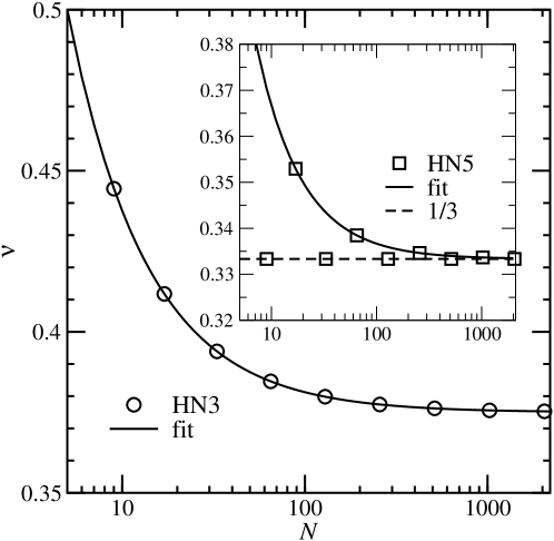
Figure 11: Highest density $\nu$ of the lattice gas on Hanoi networks found in the Monte Carlo simulation as a function of system size $N$. The main plot shows HN3, the inset shows HN5. The solid lines represent fits to powers laws according to Eq. (45), see Tab. 4. The dashed horizontal line in the inset marks the value $1/3$.

The resulting values are displayed in Tab. 4. Note that for HN5, we fitted only even powers $k$, since odd powers result in highest densities of exactly $\nu=\frac{1}{3}$. The resulting values $\nu_{\infty}$ agree precisely with the analytical results $\frac{3}{8}$ and $\frac{1}{3}$ for HN3 and HN5, respectively. Also the coefficients describing the finite-size corrections seem to be rational numbers $b=\frac{5}{8}$ and $c=-1$ for HN3 and $b=\frac{1}{3}$ and $c=-1$ for HN5. They can be understood in the following way, e.g., for HN3: The number of nodes is $N=2^{k}+1$, i.e, exactly one more than a power of 2. The number of occupied nodes for the highest density is exactly $\frac{3}{8}$ of the $2^{k}$ nodes plus one extra node, i.e., $N\nu(N)=\frac{3}{8}\,2^{k}+1=\frac{3}{8}\,(2^{k}+1)+\frac{5}{8}$ which results in $\nu(N)=\frac{3}{8}+\frac{5}{8}\,N^{-1}$. In a similar way, the scaling for the HN5 graphs can be explained, where $N$ is not divisible by 3.

Network	$\nu_{\infty}$	$b$	$c$
HN3	0.3750000(2)	0.62500(2)	-1.00000(1)
HN5 ($k$ even)	0.333333(7)	0.3333(1)	-1.0000(1)

Table 4: Result of power law fits to the $\nu(N)$ data show in Fig. 11 according to Eq. (45). Note that for HN5, only the data for even powers $k$ where used.

Next, we go beyond the analytical calculations by studying the properties of the solution landscape via sampling configurations of highest density. Hence, one must ensure that configurations exhibiting the same statistical weight in Eq. (6) are sampled with the same probability or frequency. For many systems exhibiting complex solution landscapes, this is quite an effort (Hartmann, 2000a, b; Moreno et al., 2003; Mann and Hartmann, 2010).

To achieve unbiased sampling here, we always stored a configuration of the highest density of a replica visiting the highest value $\mu_{\max}$ of the chemical potential, whenever that replica previously had visited the value $\mu=0$ in the (MCMCMC) scheme. It may be said that the replica has “performed a round trip”. This means that before a replica is stored next time, it must again diffuse to $\mu=0$ and return to the highest value of $\mu$ (Neuhaus, ). Typical round-trip times range from around 20 for $N=17$ to around 20000 for $N=2049$. To test whether this procedure yields unbiased sampling, we studied small systems of size $N=33$, where, in principle, all solutions can be enumerated. For both systems, HN3 and HN5, we sampled $10^{6}$ configurations of highest density and counted how often each configuration was found. The resulting histograms appear very flat, see Fig. 12. Hence the sampling seems to work very well, at least for Hanoi graphs.

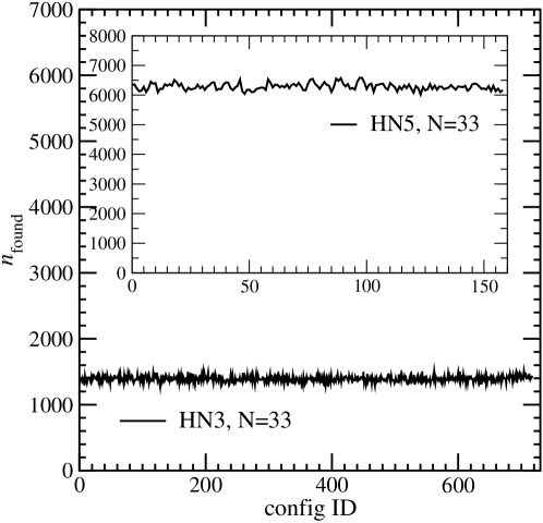
Figure 12: Histogram of how often each configuration of highest density is sampled during the (MC)³ simulation of a $N=33$ node graph for HN3 (main plot) and HN5 (inset). The total number of sampled configurations was $10^{6}$ in both cases.

Next, we study the configuration-landscape of the hard-core lattice gas at the highest density. For this purpose we take, for each value $N$ of the system size, a set of $K=200$ randomly sampled configurations of highest density. We applied a clustering algorithm to each set, to generate a hierarchical tree (“dendrogram”) representation such that “similar” configurations are grouped closer to each other than less similar configurations. As a measure of similarity between two configurations $\{x_{i}^{(\alpha)}\}$ and $\{x_{i}^{(\beta)}\}$, we simply use the normalized Hamming distance

$$d(\{x_{i}^{(\alpha)}\},\{x_{i}^{(\beta)}\})=\frac{1}{N}\sum_{i}\delta_{x_{i}^{(\alpha)},x_{i}^{(\beta)}}\,.$$ (46)

We apply the clustering algorithm of Ward (Jain and Dubes, 1988), which has already been applied to the analysis of phase-space structures (Hed et al., 2001; Barthel and Hartmann, 2004; Mann and Hartmann, 2010) (see Ref. (Hed et al., 2001) for details). The resulting dendrograms are shown in Fig. 13. The configurations are located at the leafs of the dendrogram, at the top of each dendrogram. Arranging the configurations from left to right as they appear in a dendrogram, a certain order of configurations is given. Note that the order is not unique, since for any node of the tree, the two subtrees can be exchanged without changing the clustering. Nevertheless, exchanging two subtrees has no effect on the final results. Note that any set of vectors can be clustered and represented hierarchically in this way. This is possible even for a set of purely random binary-valued vectors.

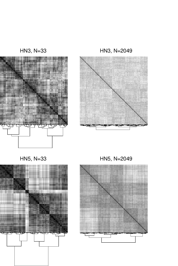
Figure 13: Distance-distance matrices for sets of $K=200$ randomly sampled highest-density configurations. The columns and rows are labeled by configurations; the order of the configurations in the rows and columns is the same and is obtained via a clustering approach (see the text). The clustering structure is visible by way of the trees (“dendrograms”) which are shown below the matrices. The entries of each matrix are normalized Hamming distances between different configurations, shown in gray scale (black indicates distance 0, white indicates distance 1).

Whether this hierarchical clustering represents the original landscape structure well, can be investigated in the following way. One draws the matrix of Hamming distances by using the order of the configurations to order the rows and columns of the matrix. If, e.g., one takes a set of suitably large, random binary-valued vectors, the resulting matrices would appear basically gray, showing that the order imposed by the clustering is artificial in this case. In Fig. 13 the Hamming-distance matrices are shown for a couple of sample systems. For both cases, HN3 and HN5, at small system sizes, a complex block-diagonal structures is visible, such that each visible block exhibits a similar substructure. This gives the impression of a complex hierarchical organization of the configuration space. Nevertheless, when going to larger system sizes, the matrices exhibit much less contrast, which strongly indicates that for $N\to\infty$ the solution landscape will be similar to a set of random vectors, i.e., without any complex organization.

This result is supported when computing the cophenetic correlations, which measure the correlation between the Hamming distances $d$ and the distances $d_{c}$ along the dendrogram

$${\cal K}\equiv[d\,d_{c}]-[d][d_{c}]\,,$$ (47)

where $[\ldots]$ is the average over pairs of configurations. Note that $d_{c}$ is the sum of the Hamming distances along a path in the tree connecting a pair configurations, respectively.

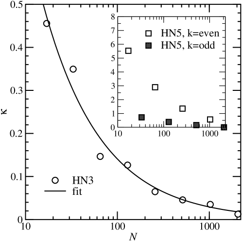
Figure 14: Cophenetic correlations in Eq. (47) as a function of system size for HN3 (main plot) and HN5 (inset). The solid line displays the function ${\cal K}(N)=3.25N^{-0.68}$.

The resulting cophenetic correlation ${\cal K}$ as a function of system size is displayed in Fig. 14. For both cases, HN3 and HN5, ${\cal K}$ decreases strongly as function of system size, taking the difference between even and odd powers $k$ for HN5 into account. For HN3, the data is compatible with a power law ${\cal K}(N)=3.25N^{-0.68}$. Hence, in the limit of infinite system sizes, the hierarchical structure imposed by the clustering is not correlated to the actual Hamming distances. This shows that the landscape of highest-density configurations appears to be simple for both HN3 and HN5, in strong contrast to the vertex-cover or lattice-gas problem on random graphs (Barthel and Hartmann, 2004).

VI Conclusions

We have succeeded in obtaining the optimal vertex coverage or packing fraction for the Hanoi networks HN3 and HN5 using the renormalization group. Our Monte Carlo simulations allowed us to confirm those results and extend them to any finite size. We have also obtained the entropy to arbitrary accuracy. We have shown that it is extensive and likely non-trivial in the sense that there is no simple generator to provide the set of all optimal configurations, a remarkable result for such a simple, planar network. It is even more remarkable that for each given size the set of all possible solutions has a complex hierarchical structure, as visible from clustering the states and considering distance-distance matrices. Nevertheless, an analysis of the cophenetic correlations shows that in the thermodynamic limit, a set of random-vector-like solutions dominates entropically and makes the solution landscape thermodynamically simple.

While there are no phase transitions in this problem, the Hanoi networks would allow one to study analytically an interesting percolation transition when considering an interpolation between the network’s one-dimensional backbone alone (a simple bipartite lattice with just two perfect solutions of 1/2 coverage) and the full network (with an extensive set of frustrated optimal solutions of coverage 5/8 for HN3 or 2/3 for HN5) by adding the small-world edges with a probability $p$. As a technical achievement, we derived the renormalization group equations for hierarchy-dependent observables to obtain, for instance, the packing fractions provided by each level of the hierarchy in the network. Here, these observables merely reveal that higher levels of the hierarchy become very uniform (even if alternating) in coverage, while most of the interesting structure resides with the majority of variables at a few lowest levels, in accordance with the numerical study of the ultrametric relation between solutions. Nevertheless, similar techniques might be useful to provide insights into the “patchy” nature of ordering on whole classes of hierarchical networks in other problems (Hinczewski and Berker, 2006; Hinczewski, 2007; Boettcher et al., 2009; Boettcher and Brunson, ; Hasegawa et al., 2010).

Appendix

A: Determining the RG-Recursion Equations

In the derivation of the recursive form of the partition function in Sec. IV, we use Eq. (IV) to transform $\Theta$ into the Ising-like form with Boolean variables $x,y,z$

$$\Theta\left(\mu_{1},x,y,z\right) = 1+e^{\mu_{1}}\left(1-y\right)\left(2-x-z\right).$$ (48)

$$= \exp\left\{2I+\frac{1}{2}G\left[\left(x+y\right)+\left(y+z\right)\right]+\frac{1}{2}H\left(x+z\right)+K\left(xy+yz\right)+Lxz+Dxyz\right\}$$

$$= C_{1}^{-2}\gamma_{1}^{-\frac{1}{2}\left[\left(x+y\right)+\left(y+z\right)\right]}\eta_{1}^{-\frac{1}{2}\left(x+z\right)}\kappa_{1}^{-\left(xy+yz\right)}\lambda_{1}^{-xz}\Delta_{1}^{-xyz},$$

where we have defined the convenient “activity” parameters

$$C=e^{-I},\quad\gamma=e^{-G},\quad\eta=e^{-H},\quad\kappa=e^{-K},\quad\lambda=e^{-L},\quad\Delta=e^{-D}.$$ (49)

Equation (48) matches Eq. (IV) for the choice of

$$C_{1}=\frac{m_{1}}{2+m_{1}}, \gamma_{1}=\frac{2+m_{1}}{m_{1}},\qquad\eta_{1}=\frac{m_{1}\left(2+m_{1}\right)}{\left(1+m_{1}\right)^{2}},$$

$$\kappa_{1}=\frac{1+m_{1}}{2+m_{1}}, \lambda_{1}=\frac{\left(1+m_{1}\right)^{2}}{m_{1}\left(2+m_{1}\right)},\qquad\Delta_{1}=\frac{m_{1}\left(2+m_{1}\right)}{\left(1+m_{1}\right)^{2}},$$ (50)

(with $m_{1}=e^{-\mu_{1}}$), which serves as the initial conditions for the renormalization-group flow for both HN3 and HN5.

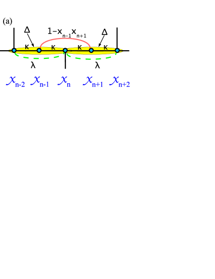
Figure 15: Depiction of the graph-lets associated with the sectional partition function $\zeta_{i}^{l}$ in Eq. (A: Determining the RG-Recursion Equations) during one RG step on HN3. The step consists of tracing out odd-labeled variables $x_{n\pm 1}$ (taking into account the hard-core constraint relevant at this level) in (a) and expressing the renormalized couplings $\left(\gamma^{\prime},\eta^{\prime},\kappa^{\prime},\lambda^{\prime},\Delta^{\prime}\right),$ in (b) in terms of the old couplings $\left(\gamma,\eta,\kappa,\lambda,\Delta\right)$. To save space, the one-point couplings (“bond magnetizations” (McKay and Berker, 1984)) $\gamma$ and $\eta$ have been omitted. These drawings summarize the calculations in Eqs. (A: Determining the RG-Recursion Equations) and (52).

In terms of these renormalization-group parameters one can then show for HN3 that the “sectional” partition functions $\zeta$ have to be written as

$$\zeta_{i}^{l}\left(x,y,z\right) = \sum_{a}\sum_{b}C_{i}^{-2}m_{i+1}^{-a-b}\gamma_{i}^{-\frac{1}{2}\left[\left(x+a\right)+\left(a+y\right)+\left(y+b\right)+\left(b+z\right)\right]}\eta_{i}^{-\frac{1}{2}\left[\left(x+y\right)+\left(y+z\right)\right]}$$

$$\qquad\kappa_{i}^{-\left(xa+ay+yb+bz\right)}\lambda_{i}^{-\left(xy+yz\right)}\Delta_{i}^{-\left(xay+ybz\right)}\left(1-ab\right),$$

$$= C_{i+1}^{-1}\gamma_{i+1}^{-\frac{1}{2}\left[\left(x+y\right)+\left(y+z\right)\right]}\eta_{i+1}^{-\frac{1}{2}\left(x+z\right)}\kappa_{i+1}^{-\left(xy+yz\right)}\lambda_{i+1}^{-xz}\Delta_{i+1}^{-xyz},$$

for which we have depicted the tracing operation graphically in Fig. 15. This operation requires that, for HN3, the renormalized quantities at $i+1$ be expressed in terms of those at $i$ with the RG recursions

$$C_{i+1}=\frac{m_{i+1}\gamma_{i}C_{i}^{2}}{2+m_{i+1}\gamma_{i}}, \gamma_{i+1}=\gamma_{i}\eta_{i}\kappa_{i}\frac{2+m_{i+1}\gamma_{i}}{2+m_{i+1}\gamma_{i}\kappa_{i}},$$

$$\eta_{i+1}=\kappa_{i}\frac{\left(2+m_{i+1}\gamma_{i}\right)\left(2+m_{i+1}\gamma_{i}\kappa_{i}\right)}{\left(1+\kappa_{i}+m_{i+1}\gamma_{i}\kappa_{i}\right)^{2}}, \kappa_{i+1}=\lambda_{i}\Delta_{i}\frac{\left(2+m_{i+1}\gamma_{i}\kappa_{i}\right)\left(1+\kappa_{i}+m_{i+1}\gamma_{i}\kappa_{i}\right)}{\left(2+m_{i+1}\gamma_{i}\right)\left(1+\kappa_{i}\Delta_{i}+m_{i+1}\gamma_{i}\kappa_{i}^{2}\Delta_{i}\right)},$$ (52)

$$\lambda_{i+1}=\frac{\left(1+\kappa_{i}+m_{i+1}\gamma_{i}\kappa_{i}\right)^{2}}{\kappa_{i}\left(2+m_{i+1}\gamma_{i}\right)\left(2+m_{i+1}\gamma_{i}\kappa_{i}\right)}, \Delta_{i+1}=\frac{\left(2+m_{i+1}\gamma_{i}\right)\left(1+\kappa_{i}\Delta_{i}+m_{i+1}\gamma_{i}\kappa_{i}^{2}\Delta_{i}\right)^{2}}{\Delta_{i}\left(2+m_{i+1}\gamma_{i}\kappa_{i}^{2}\Delta_{i}\right)\left(1+\kappa_{i}+m_{i+1}\gamma_{i}\kappa_{i}\right)^{2}}.$$

For HN5, we obtain, correspondingly,

$$\zeta_{i}^{l}\left(x,y,z\right) = \sum_{a}\sum_{b}C_{i}^{-2}m_{i+1}^{-a-b}\gamma_{i}^{-\frac{1}{2}\left[\left(x+a\right)+\left(a+y\right)+\left(y+b\right)+\left(b+z\right)\right]}\eta_{i}^{-\frac{1}{2}\left[\left(x+y\right)+\left(y+z\right)\right]}$$

$$\qquad\kappa_{i}^{-\left(xa+ay+yb+bz\right)}\lambda_{i}^{-\left(xy+yz\right)}\Delta_{i}^{-\left(xay+ybz\right)}\left(1-ab\right)\left(1-xa\right)\left(1-ay\right)\left(1-yb\right)\left(1-bz\right),$$

$$= C_{i+1}^{-1}\gamma_{i+1}^{-\frac{1}{2}\left[\left(x+y\right)+\left(y+z\right)\right]}\eta_{i+1}^{-\frac{1}{2}\left(x+z\right)}\kappa_{i+1}^{-\left(xy+yz\right)}\lambda_{i+1}^{-xz}\Delta_{i+1}^{-xyz},$$

a procedure that is graphically depicted in Fig. 16. Those extra repulsion terms in HN5 then lead to dramatically simpler RG recursions than in Eq. (52):

$$C_{i+1}=\frac{m_{i+1}\gamma_{i}C_{i}^{2}}{2+m_{i+1}\gamma_{i}}, \gamma_{i+1}=\eta_{i}\frac{2+m_{i+1}\gamma_{i}}{m},\qquad\eta_{i+1}=\frac{m_{i+1}\gamma_{i}\left(2+m_{i+1}\gamma_{i}\right)}{\left(1+m_{i+1}\gamma_{i}\right)^{2}},$$ (54)

$$\kappa_{i+1}=\lambda_{i}\frac{\left(1+m_{i+1}\gamma_{i}\kappa_{i}\right)}{\left(2+m_{i+1}\gamma_{i}\right)}, \lambda_{i+1}=\frac{\left(1+m_{i+1}\gamma_{i}\right)^{2}}{m_{i+1}\gamma_{i}\left(2+m_{i+1}\gamma_{i}\right)},\qquad\Delta_{i+1}=\frac{m_{i+1}\gamma_{i}\left(2+m_{i+1}\gamma_{i}\right)}{\left(1+m_{i+1}\gamma_{i}\right)^{2}}.$$

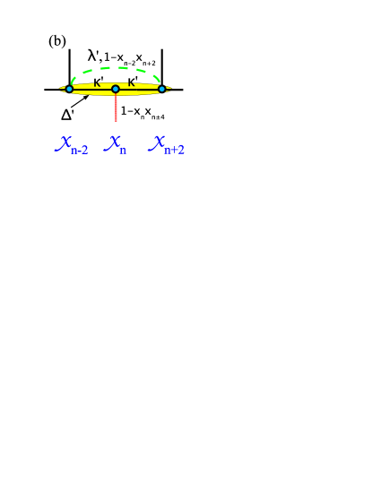
Figure 16: Depiction of the (exact) RG step on HN5. This step is identical to that for HN3 in Fig. 15 aside from the additional hard-core repulsive terms in (a) between $x_{n\pm 2}$ and $x_{n}$ which is relevant for the current RG step, and in (b) between $x_{n-2}$ and $x_{n+2}$ which contributes at the next level of the RG.

For the discussion in Appendix B, it is useful to defined the vector of renormalizable parameters,

$$\vec{A}_{i}\left(m_{1},\ldots,m_{i}\right) = \left(C_{i},\gamma_{i},\eta_{i},\kappa_{i},\lambda_{i},\Delta_{i}\right),$$ (55)

where at each level of the RG $i$ depends implicitly, through the renormalized parameters, on the first $i$ values of the chemical potentials, as in Eq. (18) for the initial case $i=1$, for example. In the analysis, we will symbolically refer to these renormalization group equations formally as a (nonlinear) operator,

$$\vec{A}_{i+1}\left(m_{1},\ldots,m_{i+1}\right)= \vec{{\cal R}}_{m_{i+1}} \left[\vec{A}_{i}\left(m_{1},\ldots,m_{i}\right)\right],$$ (56)

highlighting the fact that the RG transforms depend explicitly on the parameters $m_{i+1}$.

B. Hierarchical Packing Fraction

For later use, we follow convention in defining the Jacobian matrix derived from a formal derivation of the renormalization group equations as defined in Eqs. (55,56),

$$\overleftrightarrow{W}\left(\vec{A}_{i}\right) = \frac{\partial\vec{A}_{i+1}}{\partial\vec{A}_{i}}=\frac{\partial\vec{{\cal R}}_{\mu_{i+1}}\left(\vec{A}_{i}\right)}{\partial\vec{A}_{i}}=\frac{\partial\left(C_{i+1},\gamma_{i+1},\eta_{i+1},\kappa_{i+1},\lambda_{i+1},\Delta_{i+1}\right)}{\partial\left(C_{i},\gamma_{i},\eta_{i},\kappa_{i},\lambda_{i},\Delta_{i}\right)}.$$ (57)

Using the fundamental statement for the grand partition function $\Xi^{(k)}$ of the unrenormalized system (or the free energy $f^{(k)}=2^{-k}\ln\Xi^{(k)}$, instead) in terms of the renormalized partition functions $Z^{(i<k)}$ in Eq. (IV.2), we can find for the specific packing fraction in the $i$-th level of the hierarchy

$$\nu_{i}\left(\vec{\mu}\right) = \frac{1}{2^{k}}\left\langle\sum_{j=1}^{2^{k-i}}x_{2^{i}\left(2j-1\right)}\right\rangle=\frac{\partial f^{(k)}}{\partial\mu_{i}}=-2^{-k}m_{i}\frac{d}{dm_{i}}\ln\Xi^{(k)},$$ (58)

implicitly defining the hierarchy-specific chemical potential $m_{i}=e^{\mu_{i}}$ in the form of the vector

$$\vec{m} = \left(m_{1},m_{2},\ldots,m_{k}\right).$$ (59)

Applying such a derivative to the sequence in Eq. (IV.2), we obtain for $1\leq i<k$

$$\frac{d}{dm_{i}}\ln\Xi^{(k)}\left(m_{1},m_{2},\ldots,m_{k}\right) = \frac{d}{dm_{i}}\ln Z^{(1)}\left[\vec{A}_{k-1}\left(m_{1},\ldots,m_{k-1}\right),m_{k}\right]=\frac{\partial\ln Z^{(1)}\left[\vec{A}_{k-1},m_{k}\right]}{\partial\vec{A}_{k-1}}\circ\frac{d\vec{A}_{k-1}}{dm_{i}}.$$ (60)

We can understand the progression of derivatives in Eq. (60) from the result in Eq. (56),

$$\frac{d\vec{A}_{l}}{dm_{i}} = \frac{d}{dm_{i}}\vec{{\cal R}}_{m_{l}}\left[\vec{A}_{l-1}\left(m_{1},\ldots,m_{l-1}\right)\right]=\begin{cases}\frac{\partial\vec{{\cal R}}_{m_{i}}}{\partial m_{i}}\left[\vec{A}_{i-1}\left(m_{1},\ldots,m_{i-1}\right)\right],&i=l,\\ \overleftrightarrow{W}\left(\vec{A}_{l-1}\right)\circ\frac{d\vec{A}_{l-1}\left(m_{1},\ldots,m_{l-1}\right)}{dm_{i}},&i<l,\\ 0,&i>l,\end{cases}$$ (61)

using, from Eq. (57), the matrix

$$\overleftrightarrow{W}\left(\vec{A}_{l}\right) = \frac{\partial\vec{{\cal R}}_{m_{l+1}}}{\partial\vec{A}}\left[\vec{A}_{l}\left(m_{1},\ldots,m_{l}\right)\right].$$ (62)

Note that the distinction between the implicit and explicit derivatives in Eq. (61) results from the explicit occurrence of $m_{i}$ just that once in the $i$-th RG step in the recursions and that afterward the parameters being renormalized depend implicitly on $m_{i}$. Thus, application of the relation in Eq. (61), repeatedly for all $l>i$ and once, finally, for $l=i$, yields

$$\frac{d}{dm_{i}}\ln\Xi^{(k)}\left(m_{1},\ldots,m_{k}\right)=\frac{\partial\ln Z^{(1)}}{\partial\vec{A}}\left(\vec{A}_{k-1},m_{k}\right)\circ\overleftrightarrow{W}\left(\vec{A}_{k-2}\right)\circ\ldots\circ\overleftrightarrow{W}\left(\vec{A}_{i}\right)\circ\frac{\partial\vec{{\cal R}}_{m}}{\partial m}\left[\vec{A}_{i-1}\left(m_{1},\ldots,m_{i-1}\right)\right].$$ (63)

Now it is easy to set all chemical activities equal, $m_{i}=m$, with $1\leq i\leq k$, irrespective of which hierarchy was targeted, to get

$$\left.\frac{d}{dm_{i}}\ln\Xi^{(k)}\left(m_{1},\ldots,m_{k}\right)\right|_{m_{i}\equiv m}=\begin{cases}\frac{\partial\ln Z^{(1)}}{\partial\vec{A}}\left(\vec{A}_{k-1},m\right)\circ\overleftrightarrow{W}\left(\vec{A}_{k-2}\right)\circ\ldots\circ\overleftrightarrow{W}\left(\vec{A}_{i}\right)\circ\frac{\partial\vec{{\cal R}}_{m}}{\partial m}\left(\vec{A}_{i-1}\right),&1\leq i<k,\\ \frac{\partial\ln Z^{(1)}}{\partial m}\left(\vec{A}_{k-1},m\right),&i=k.\end{cases}$$ (64)

We can relate this procedure back to that for the total occupation defined in Eq. (7) using a uniform $m$. To this end, we define an extended vector of parameters with an explicit $m$-dependence

$$\vec{A^{\prime}}_{i} = \left(\vec{A}_{i},m\right)=\left(C_{i},\gamma_{i},\eta_{i},\kappa_{i},\lambda_{i},\Delta_{i},m\right).$$ (65)

Then

$$\frac{d}{dm}\vec{A^{\prime}}_{i}=\left(\frac{d}{dm}\vec{A}_{i},\frac{dm}{dm}\right)=\left(\overleftrightarrow{W}\left(\vec{A}_{i-1}\right)\circ\frac{d}{dm}\vec{A}_{i-1}+\frac{\partial{\cal\vec{R}}_{m}}{\partial m}\left(\vec{A}_{i-1}\right),1\right)=\overleftrightarrow{W^{\prime}}\left(\vec{A}_{i-1}\right)\circ\frac{d}{dm}\vec{A^{\prime}}_{i-1},$$ (66)

with the extended Jacobian matrix

$$\overleftrightarrow{W^{\prime}}\left(\vec{A}_{i-1}\right) = \left[\begin{array}[]{cc}\frac{\partial\vec{A}_{i}}{\partial\vec{A}_{i-1}},&\frac{\partial\vec{A}_{i}}{\partial m}\\ \frac{\partial m}{\partial\vec{A}_{i-1}},&\frac{\partial m}{\partial m}\end{array}\right]=\left[\begin{array}[]{cc}\overleftrightarrow{W}\left(\vec{A}_{i-1}\right),&\frac{\partial{\cal\vec{R}}_{m}}{\partial m}\left(\vec{A}_{i-1}\right)\\ 0,&1\end{array}\right].$$ (71)

According to Eqs. (7) and (58) we have $\nu=\sum_{i=1}^{k}\nu_{i}$, so

$$\frac{d}{dm}\ln\Xi^{(k)}\left(m\right)=\sum_{i=1}^{k}\left.\frac{d}{dm_{i}}\ln\Xi^{(k)}\left(m_{1},\ldots,m_{k}\right)\right|_{m_{i}\equiv m}$$ (72)

$$= \frac{\partial\ln Z^{(1)}}{\partial m}\left(\vec{A}_{k-1},m\right)+\frac{\partial\ln Z^{(1)}}{\partial\vec{A}}\left(\vec{A}_{k-1},m\right)\circ\sum_{i=1}^{k-1}\overleftrightarrow{W}\left(\vec{A}_{k-2}\right)\circ\ldots\circ\overleftrightarrow{W}\left(\vec{A}_{i}\right)\circ\frac{\partial\vec{{\cal R}}_{m}}{\partial m}\left(\vec{A}_{i-1}\right)$$

$$= \frac{\partial\ln Z^{(1)}}{\partial m}\left(\vec{A}_{k-1},m\right)+\frac{\partial\ln Z^{(1)}}{\partial\vec{A}}\left(\vec{A}_{k-1},m\right)$$

$$\,\circ\left[\overleftrightarrow{W}\left(\vec{A}_{k-2}\right)\circ\left[\ldots\left[\overleftrightarrow{W}\left(\vec{A}_{2}\right)\circ\left[\overleftrightarrow{W}\left(\vec{A}_{1}\right)\circ\frac{\partial\vec{{\cal R}}_{m}}{\partial m}\left(\vec{A}_{0}\right)+\frac{\partial\vec{{\cal R}}_{m}}{\partial m}\left(\vec{A}_{1}\right)\right]+\frac{\partial\vec{{\cal R}}_{m}}{\partial m}\left(\vec{A}_{2}\right)\right]\ldots\right]+\frac{\partial\vec{{\cal R}}_{m}}{\partial m}\left(\vec{A}_{k-2}\right)\right]$$

$$= \frac{\partial\ln Z^{(1)}}{\partial m}\left(\vec{A^{\prime}}_{k-1}\right)+\frac{\partial\ln Z^{(1)}}{\partial\vec{A}}\left(\vec{A^{\prime}}_{k-1}\right)\circ\overleftrightarrow{W^{\prime}}\left(\vec{A}_{k-2}\right)\circ\ldots\circ\overleftrightarrow{W^{\prime}}\left(\vec{A}_{1}\right)\circ\frac{\partial\vec{A^{\prime}}_{0}}{\partial m},$$

where the last equality follows from Eqs. (66) and (71). [Note that $\frac{\partial\vec{A^{\prime}}_{0}}{\partial m}=\left(0,1\right)$.]

C. Counting Optimal Packings

In this section we attempt to determine a set of recursions to count the number of optimal packings in HN3. In the end, we merely succeed in providing a rigorous lower bound on the entropy density. This exercise is interesting in its own right as it highlights the surprising complexity in the structure of vertex covers or particle packings on this network. The key ingredients to provide such an approach originate with the depictions of the solutions for $k=3$ and 4 in Figs. 7 and 8, and with the observation, in Sec. V, that at each finite system size $N=2^{k}+1$, exactly $3\times 2^{k-3}+1$ particles can be maximally packed into the network. Let us imagine we would try to assemble the $k=4$ solutions from those of size $k=3$: We would have to join any two solutions at one end point and add a long link between their respective midpoints; the merging point becomes the new midpoint and the respective open end points remain just that. In the process $\left(k-1\right)\to k$, we have to remove a single particle overall, as

$$2\left[3\times 2^{\left(k-1\right)-3}+1\right]-1=3\times 2^{k-3}+1.$$ (73)

In this construction, it appears that only the state of midpoints and end points is relevant, which we can denote by $\left(n_{0}n_{\frac{N}{2}}n_{N}\right)$ with $n_{i}\in\left\{0,1\right\}$, depending on whether that site is (1) or is not (0) occupied by a particle. For instance, the four solutions in Fig. 7 would be labeled $\left(110\right),\left(111\right),\left(101\right),\left(101\right)$ from left to right and then from top to bottom; we omit the reflection $\left(011\right)$ of $(110)$. In fact, a glance at Fig. 8 suggests these are the only four possibilities realized. We have directly enumerated these classes in Tab. 5.

Table 5: Distinct classes (see the text) of solutions for HN3 for each system size $N=2^{k}+1$. For each $k$, the total count adds up to the number of solutions given in Tab. 1

$k$	$\left(011\right)$	$\left(110\right)$	$\left(101\right)$	$\left(111\right)$
3	1	1	3	2
4	3	3	10	21
5	30	30	138	520
6	4140	4140	22440	162564

To construct solutions of size $k$ from those at size $k-1$, we consider all 16 pairings of these classes, which we symbolize by

$$\widehat{\left(n_{0}n_{\frac{N}{4}}n_{\frac{N}{2}}\right)\left(n_{\frac{N}{2}}n_{\frac{3N}{2}}n_{N}\right)}_{k-1}\to\left(n_{0}n_{\frac{N}{2}}n_{N}\right)_{k},$$ (74)

where the over-caret corresponds to the extra long-range edge added to connect the two former mid-points, prohibiting them from being simultaneously occupied. With that, we find the following rules:

1. Merging two end-points into a new midpoint is possible

   1. at no cost, when both are empty, i.e., $\widehat{\left(xx0)(0xx\right)}_{k-1}\to\left(x0x\right)_{k}$, making a new midpoint that is empty, or

   2. at the expense of one particle otherwise, i.e., $\widehat{\left(xx0)(1xx\right)}_{k-1}$, $\widehat{\left(xx1)(0xx\right)}_{k-1}$, or $\widehat{\left(xx1)(1xx\right)}_{k-1}\to\left(x1x\right)_{k}$.

2. Linking the two mid-points with an edge is possible

   1. at no cost, when at least one of the two mid-points is empty, or

   2. at the expense of one particle, either from the left or right mid-point, if both mid-points are occupied.

The merger can proceed only when exactly one particle gets expended, due to Eq. (73). Hence, the combinations of 1(a) with 2(b) and 1(b) with 2(a) are allowed. The eight permissible mergers that are left exactly map these four classes onto themselves:

$$\left[1.\right]\widehat{\left(011)(101\right)}_{k-1}\to\left(011\right)_{k}\qquad\left[3.\right]\widehat{\left(101)(011\right)}_{k-1}\to\left(101\right)_{k}\qquad\left[6.\right]\widehat{\left(101)(101\right)}_{k-1}\to\left(111\right)_{k}$$

$$\left[2.\right]\widehat{\left(101)(110\right)}_{k-1}\to\left(110\right)_{k}\qquad\left[4.\right]\widehat{\left(110)(101\right)}_{k-1}\to\left(101\right)_{k}\qquad\left[7.\right]\widehat{\left(101)(111\right)}_{k-1}\to\left(111\right)_{k}$$

$$\left[5.\right]\widehat{\left(110)(011\right)}_{k-1}\to\left(101\right)_{k}\qquad\left[8.\right]\widehat{\left(111)(101\right)}_{k-1}\to\left(111\right)_{k}$$ (75)

It seems straightforward now to deduce the recursions for the number of configurations in each class, from one size to the next. We define the cardinality for each set as $x_{k}\equiv\left|\left(011\right)_{k}\right|\equiv\left|\left(110\right)_{k}\right|$, $y_{k}\equiv\left|\left(101\right)_{k}\right|$, and $z_{k}\equiv\left|\left(111\right)_{k}\right|$ to obtain, from the rules in Eqs. (75),

$$x_{k} = x_{k-1}y_{k-1},$$ (76)

$$y_{k} = 2f_{k-1}x_{k-1}y_{k-1}+2g_{k-1}x_{k-1}^{2},$$

$$z_{k} = y_{k-1}^{2}+2y_{k-1}z_{k-1,}$$

with the initial conditions provided by Tab. 5: $x_{3}=1,y_{3}=3,z_{3}=2$. The recursions for $x_{k}$ and $z_{k}$ are exact, as is illustrated by evolving from one row to the next in Tab. 5. The recursion for $y_{k}$, though, can only provide a lower bound on its growth. The factors of 2 in front of both terms arises from Eq. (75), as the maps $\left[3.\right]$ and $\left[4.\right]$ provide two contributions to the first while map $\left[5.\right]$, in applying rule 2(b), gives us two ways of removing a particle in the second term. The “fudge factors” $f_{k}$ and $g_{k}$ arise because in each of these cases (and only these) the particle removal eliminates constraints on other particles in the respective subgraph, opening the door for an undetermined number of further combinations from less than optimally packed subgraphs. All we know is that these factors are larger than unity, but they could vary with $k$ to an unbounded size. For further analysis, we assume that they can at least be approximated by constants $f$ and $g$. Then, we divide the second recursion by the first in Eq. (76) to find $y_{k}/x_{k}\sim\lambda$ for $k\to\infty$, with $\lambda\equiv f+\sqrt{f^{2}+2g}\geq 1+\sqrt{3}$. It is then easy to obtain asymptotically $y_{k}\sim\lambda x_{k}\sim\left(\lambda x_{3}\right)^{2^{k-3}}$ and $z_{k}\sim 2^{k-3}\left(\lambda x_{3}\right)^{2^{k-3}}\left(1+z_{3}/y_{3}\right)$. The total number of optimal packings is then $\Omega_{k}\geq 2x_{k}+y_{k}+z_{k}\sim z_{k}$, which reduces to the entropy density

$$s_{k}\sim\frac{\ln\Omega_{k}}{2^{k}}\geq\frac{1}{8}\ln\left(\lambda x_{3}\right)\geq\frac{\ln\left(1+\sqrt{3}\right)}{8}\approx 0.1256,$$ (77)

using $x_{3}=1$ and the lowest value of $\lambda$. While this is a poor lower bound, it nonetheless establishes the extensivity of the solution-space entropy. However, its derivation also demonstrates that the structure of optimal packings is quite non-trivial in this network.

References

- Weigt and Hartmann (2000) M. Weigt and A. K. Hartmann, Phys. Rev. Lett. 84, 6118 (2000).
- Hartmann and Weigt (2005) A. K. Hartmann and M. Weigt, Phase Transitions in Combinatorial Optimization Problems (Wiley-VCH, Weinheim, 2005).
- Boettcher et al. (2008a) S. Boettcher, B. Gonçalves, and H. Guclu, J. Phys. A: Math. Theor. 41, 252001 (2008a).
- Boettcher and Goncalves (2008) S. Boettcher and B. Goncalves, Europhys. Lett. 84, 30002 (2008).
- Boettcher et al. (2008b) S. Boettcher, B. Goncalves, and J. Azaret, J. Phys. A: Math. Theor. 41, 335003 (2008b).
- Karp (1972) R. M. Karp, in Complexity of Computer Computations, edited by R. Miller and J. Thatcher (Plenum, New York, 1972), pp. 85–103.
- Weigt and Hartmann (2001) M. Weigt and A. K. Hartmann, Phys. Rev. E 63, 056127 (2001).
- Erdös and Rényi (1960) P. Erdős and A. Rényi, Publ. Math. Inst. Hungar. Acad. Sci. 5, 17 (1960).
- Watts and Strogatz (1998) D. J. Watts and S. H. Strogatz, Nature 393, 440 (1998).
- Barabasi and Albert (1999) A.-L. Barabasi and R. Albert, Science 286, 509 (1999).
- Andrade et al. (2005) J. S. Andrade, H.-J. Herrmann, R. F. S. Andrade, and L. R. da Silva, Phys. Rev. Lett. 94, 018702 (2005).
- Hinczewski and Berker (2006) M. Hinczewski and A. N. Berker, Phys. Rev. E 73, 066126 (2006).
- Zhang et al. (2007) Z. Zhang, S. Zhou, L. Fang, J. Guan, and Y. Zhang, Europhys. Lett. 79, 38007 (2007).
- Newman (2003) M. E. J. Newman, SIAM Review 45, 167 (2003).
- Barrat and Weigt (2000) A. Barrat and M. Weigt, Eur. Phys. J. B 13, 547 (2000).
- Aleksiejuk et al. (2002) A. Aleksiejuk, J. A. Holyst, and D. Stauffer, Physica A 310, 260 (2002).
- Plischke and Bergersen (1994) M. Plischke and B. Bergersen, Equilibrium Statistical Physics, 2nd edition (World Scientifc, Singapore, 1994).
- Barthelemy (2011) M. Barthelemy, Phys. Rep. 499, 1 (2011).
- Wannier (1950) G. H. Wannier, Phys. Rev. 79, 357 (1950).
- M.E.J. Newman and G.T. Barkema (1999) M.E.J. Newman and G.T. Barkema, Monte Carlo Methods in Statistical Physics (Oxford University Press, 1999).
- Jain and Dubes (1988) A. K. Jain and R. C. Dubes, Algorithms for Clustering Data (Prentice-Hall, Englewood Cliffs, NJ, 1988).
- Weigt and Hartmann (2003) M. Weigt and A. K. Hartmann, Europhys. Lett. 62, 533 (2003).
- Vázquez and Weigt (2003) A. Vázquez and M. Weigt, Phys. Rev. E 67, 027101 (2003).
- Boettcher et al. (2011) S. Boettcher, S. Varghese, and M. A. Novotny, Phys. Rev. E 83, 041106 (2011).
- Boettcher et al. (2009) S. Boettcher, J. L. Cook, and R. M. Ziff, Phys. Rev. E 80, 041115 (2009).
- (26) S. Boettcher and T. Brunson, Phys. Rev. E 83, 021103 (2011).
- Garey and Johnson (1979) M. R. Garey and D. S. Johnson, Computers and Intractability: A Guide to the Theory of NP-Completeness (W. H. Freeman, New York, 1979).
- Ausiello et al. (1999) G. Ausiello, P. Crescenzi, G. Gambosi, V. Kann, A. Marchetti-Spaccamela, and M. Protasi, Complexity and Approximation (Springer, Berlin, 1999).
- Geyer (1991) C. Geyer, in 23rd Symposium on the Interface between Computing Science and Statistics (Interface Foundation North America, Fairfax, 1991), p. 156.
- Hukushima and Nemoto (1996) K. Hukushima and K. Nemoto, J. Phys. Soc. Jpn. 65, 1604 (1996).
- Barthel and Hartmann (2004) W. Barthel and A. K. Hartmann, Phys. Rev. E 70, 066120 (2004).
- Hartmann (2009) A. K. Hartmann, Practical Guide to Computer Simulations (World Scientific, Singapore, 2009).
- Hartmann (2000a) A. K. Hartmann, J. Phys. A 33, 657 (2000a).
- Hartmann (2000b) A. K. Hartmann, Eur. Phys. J. B 13, 539 (2000b).
- Moreno et al. (2003) J. J. Moreno, H. G. Katzgraber, and A. K. Hartmann, Int. J. Mod. Phys. C 14, 285 (2003).
- Mann and Hartmann (2010) A. Mann and A. K. Hartmann, Phys. Rev. E 82, 056702 (2010).
- (37) T. Neuhaus, private communication.
- Hed et al. (2001) G. Hed, A. K. Hartmann, D. Stauffer, and E. Domany, Phys. Rev. Lett. 86, 3148 (2001).
- Hinczewski (2007) M. Hinczewski, Phys. Rev. E 75, 061104 (2007).
- Hasegawa et al. (2010) T. Hasegawa, T. Nogawa, and K. Nemoto, arXiv:eprint 1009.6009.
- McKay and Berker (1984) S. R. McKay and Berker, Phys. Rev. B 29, 1315 (1984).