Beyond The Standard Model:
Some Aspects of
Supersymmetry and Extra Dimension

ACKNOWLEDGMENTS

I gratefully acknowledge the academic and personal support received from my supervisor Prof. Gautam Bhattacharyya. He has been the friend, philosopher and guide, in its truest sense. I thank him for the infinite patience, with which he discussed and addressed all my problems in physics and beyond. I shall remain indebted to Prof. Amitava Raychaudhuri and Prof. Palash Baran Pal from whom I learned the basics of particle physics and received vital guidance, that navigated me through the labyrinth of my early research life. I also thank Prof. Probir Roy for his encouragement and guidance.

It is my great pleasure to thank Prof. Tapan Kumar Das, Prof. Subinay Dasgupta and Prof. Anirban Kundu from the University of Calcutta and Prof. Partha Majumdar, Prof. Pijushpani Bhattacharjee and Prof. Kamalesh Kar from Saha Institute of Nuclear Physics for their encouragement and support at different stages of my PhD work. I thank Prof. Stephane Lavignac of IPhT, CEA-Saclay, for reading the manuscript, pointing out mistakes and suggesting improvements. I thank Dr. Swarup Kumar Majee, Biplob Bhattacharjee and Kirtiman Ghosh for their collaborations and insightful discussions on the nuances of particle physics. I am grateful to SINP, and all its members, for providing an enriching and friendly environment to carry out my research. I would specifically like to thank all the academic members, the non-academic members and the research scholars of Theory Division at SINP for their continued encouragements and support. I would like to acknowledge the Council of Scientific and Industrial Research, India for the S. P. Mukherjee Fellowship.

When the going got tough in physics, my friends pulled me through. I thank Bappa, Abhiroop, Gopal, Pappu, Sumon, Arnab, Samriddhi, Purbasha and Sourav, for all the eagerly awaited adda sessions. I fondly remember the regular discussions, the occasional debates and the rare fights, that I had with Abhishek , on science, politics, cricket, films and everything else.

This thesis is dedicated to my grand mother Late (Mrs.) Sadhana Ray.

This work would not have been possible without the inspiration and encouragements of my father Prof. Siddhartha Ray and the unconditional love of my mother Mrs. Dipali Ray. I shall remember with humility all the sacrifices they made for me. I am grateful for the love and affection bestowed on me by my brother, Mr. Ananda Ray and his wife, Mrs. Arpita Ray. It remains to name my fiercest critic and my closest aide; my life support system, my wife, Srirupa.

Tirtha Sankar Ray

Kolkata, India

This thesis is partially based on the following publications

• Radiative correction to the lightest neutral Higgs mass in warped supersymmetry
  Authors: G. Bhattacharyya, S. K. Majee and T. S. Ray
  Published in: Phys. Rev.  D 78 (2008) 071701 (Rapid communication)
  e-Print: arXiv:0806.3672 [hep-ph]

• Probing warped extra dimension via ${gg\to h}$ and ${h\to\gamma\gamma}$ at LHC
  Authors: G. Bhattacharyya and T. S. Ray
  Published in: Phys. Lett.  B 675 (2009) 222
  e-Print: arXiv:0902.1893 [hep-ph]

• A phenomenological study of 5d Supersymmetry
  Authors: G. Bhattacharyya and T. S. Ray
  Published in: JHEP 1005 (2010) 040
  e-Print: arXiv:1003.1276 [hep-ph]

Chapter 1 Introduction

Particle physics endeavors to provide a description of fundamental particles and their interactions in the quantum realm. Intense experimental investigations and clairvoyant theoretical innovations in the last century culminated in the formulation of the Standard Model of particle physics. It bloomed from the ideas originally put forward by S. L. Glashow, S. Wienberg and A. Salam [2] in the 1960’s. Decades of increasingly intense experimental scrutiny has put this theory on strong footing. Today it is believed that the Gauge Field Theoretic [1] language of the Standard Model (SM) is the right path to describe quantum particle interactions. The notion of theoretic consistancy, cosmological observations like the detection of dark matter etc. indicate that the SM only provides a partial picture of the fundamental particles. Nevertheless, any extensions of this theory must closely resemble the SM at the energies that have already been explored at collider and other laboratory experiments.

1.1 The Standard Model

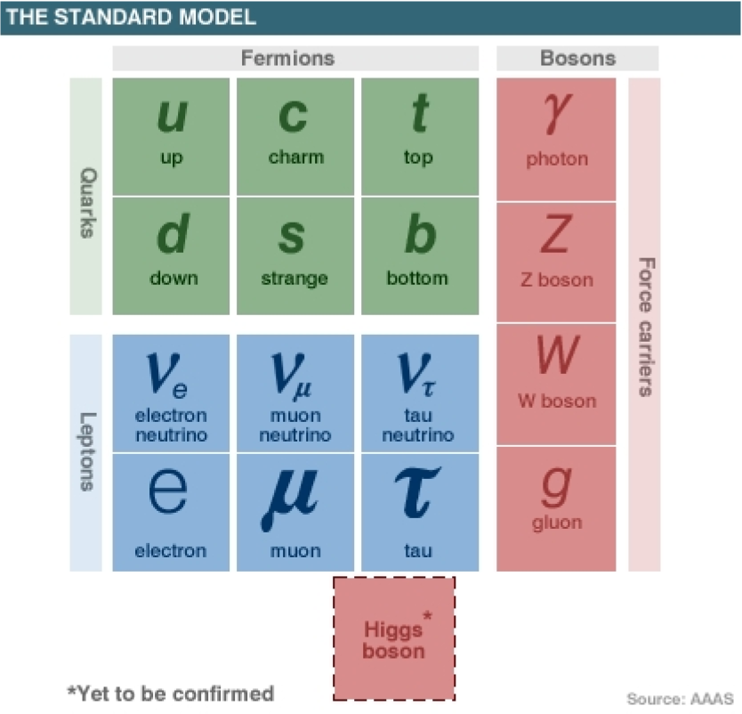
Figure 1.1: The particle content of the Standard Model.

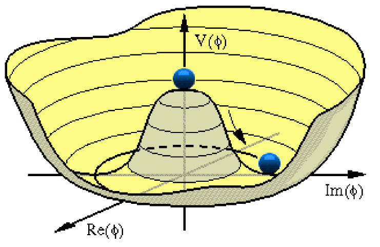
Figure 1.2: The Higgs potential in the Standard Model.

The particle content of the Standard Model was discovered at the various collider experiments. The last particle to be discovered is the Top quark, discovered at the Tevatron. The Higgs field which is an integral part of the theory has evaded discovery till the date of writing this thesis. The so called zoo of fundamental particles is summarized in Figure 1.2.

The Standard Model (SM) is a specific form of a gauge field theory with a gauge group of $SU(3)_{c}\times SU(2)_{L}\times U(1)_{Y}$. It provides a unified picture of the strong, weak and electromagnetic interactions. The $SU(3)_{c}$ part of the gauge group exclusively describes the strong interactions and is independently called Quantum Chromo Dynamics (QCD). Whereas the $SU(2)_{L}\times U(1)_{Y}$ part of the gauge group provides a unified picture of the electromagnetic and the weak interactions and is called the Electroweak sector of the theory.

The strong interaction part, or the (QCD) [3] has an $SU(3)$ gauge group. The Lagrangian density may be written as,

$$\mathcal{L}_{QCD}=-\frac{1}{4}G^{i}_{\mu\nu}G^{i\mu\nu}+\sum_{r}\bar{q}_{r\alpha}i\not{\!\!D}^{\alpha}_{\beta}\,q^{\beta}_{r},$$ (1.1)

where,

$$G^{i}_{\mu\nu}=\partial_{\mu}G^{i}_{\nu}-\partial_{\nu}G^{i}_{\mu}-g_{s}f_{ijk}\;G_{\mu}^{j}\;G_{\nu}^{k}$$ (1.2)

is the field strength tensor for the gluon fields $G^{i}_{\mu},\;i=1,\cdots,8$, $g_{s}$ is the QCD gauge coupling constant and the structure constants $f_{ijk}$ $(i,j,k=1,\cdots,8)$ are defined by

$$[\lambda^{i},\lambda^{j}]=2if_{ijk}\lambda^{k},$$ (1.3)

where the $\lambda$ are the $SU(3)$ generator matrices normalized by $\mbox{Tr}\,\lambda^{i}\lambda^{j}=2\delta^{ij}$, so that $\mbox{Tr}\,[\lambda^{i},\lambda^{j}]\lambda^{k}=4if_{ijk}$.

The $G^{2}$ term leads to the self-interaction of gluons. The second term in $\mathcal{L}_{QCD}$ is the gauge covariant derivative for the quarks: $q_{r}$ is the $r^{th}$ quark flavor, $\alpha,\beta=1,2,3$ are color indices, and

$$D^{\alpha}_{\mu\beta}=(D_{\mu})_{\alpha\beta}=\partial_{\mu}\delta_{\alpha\beta}+ig_{s}\;G^{i}_{\mu}\;L^{i}_{\alpha\beta},$$ (1.4)

where the quarks transform according to the triplet representation matrices $L^{i}={\lambda^{i}}/{2}$. The color interactions are diagonal in the flavor indices, but in general change the quark colors. These interactions are purely vector like and thus parity conserving. There are in addition, effective ghost and gauge-fixing terms which enter into the quantization of both the $SU(3)$ and electroweak parts of the theory. In the QCD part of the theory, there is the possibility of adding a (unwanted) term which violates $CP$ invariance. QCD has the property of asymptotic freedom [4], i.e., the coupling becomes weak at high energies enabling perturbative study at these energy scales or short distances. At low energies or large distances it becomes strongly coupled [5] which is sometimes called infrared slavery, leading to the confinement of quarks and gluons. The confinement of quarks and gluons is still an ill-understood facet of QCD as it is riddled with the difficulty of being a non-perturbative phenomenon. Note that there are no tree level mass terms for the quarks in the Lagrangian given in Eq. 1.1. These would be allowed by QCD alone, but are forbidden by the chiral symmetry of the electroweak part of the theory. The quark masses are generated by phenomenon of spontaneous electroweak symmetry breaking.

The theoretical picture of QCD described above was painstakingly verified through various collider experiments. The scaling of structure functions in the deep inelastic collisions of nucleons provided the first glimpse of hadronic substructure, parton model of hadrons was invoked to explain this phenomenon. The scaling violations that were discovered later provided indirect verification of perturbative QCD. Though QCD is a vast subject by itself and is an integral part of present quest for a quantum description of particle interaction, it is not the main subject of study in this thesis and it will not be explored any further in what follows.

The gauge group of the electroweak sector is the $SU(2)_{L}\times U(1)_{Y}$. The constituents of the SM fall into valid representation of these groups. An important feature of this model is the chiral nature of the interactions. Unlike QCD, the left and right chiral parts of the fields behave differently under the electroweak gauge transformation. This phenomenon can be consistently described by using the following representations of the field. We represent the leptonic sector of the electroweak theory by the left-handed leptons

$$\mathsf{L}_{1}=\left(\begin{array}[]{c}\nu_{e}\\ e^{-}\end{array}\right)_{\mathrm{L}}\;\;\mathsf{L}_{2}=\left(\begin{array}[]{c}\nu_{\mu}\\ \mu^{-}\end{array}\right)_{\mathrm{L}}\;\;\mathsf{L}_{3}=\left(\begin{array}[]{c}\nu_{\tau}\\ \tau^{-}\end{array}\right)_{\mathrm{L}}\;,$$ (1.5)

with weak isospin $I=1/2$ and weak hypercharge $Y(\mathsf{L}_{i})=-1$, corresponding to the $SU(2)$ and $U(1)$ charges respectively. The right-handed weak-isoscalar charged leptons are represented by

$$\mathsf{E}_{1,2,3}=e_{\mathrm{R}},\mu_{\mathrm{R}},\tau_{\mathrm{R}}\;,$$ (1.6)

with weak hypercharge $Y(\mathsf{E}_{i})=-2$. The right handed fields are singlets under $SU(2)$. The weak hypercharges are chosen to reproduce the observed electric charges, through the connection $Q=I_{3}+1/2Y$. The original Glashow-Wienberg-Salam model did not have a right chiral neutrino, leaving the neutrinos massless.

The hadronic sector consists of the left-handed quarks

$$\mathcal{Q}_{1}=\left(\begin{array}[]{c}u\\ d\end{array}\right)_{\mathrm{L}}\;\;\mathcal{Q}_{2}=\left(\begin{array}[]{c}c\\ s\end{array}\right)_{\mathrm{L}}\;\;\mathcal{Q}_{3}=\left(\begin{array}[]{c}t\\ b\end{array}\right)_{\mathrm{L}}\;,$$ (1.7)

with weak isospin $I=1/2$ and weak hypercharge $Y(\mathcal{Q}_{i})=1/3$, and their right-handed weak-isoscalar counterparts

$$\mathcal{U}_{(1,2,3)}=u_{\mathrm{R}},c_{\mathrm{R}},t_{\mathrm{R}}\hbox{ and }\mathcal{D}_{(1,2,3)}=d_{\mathrm{R}},s_{\mathrm{R}},b_{\mathrm{R}}\;,$$ (1.8)

with weak hypercharges $Y(\mathcal{U}_{i})=4/3$ and $Y(\mathcal{D}_{i})=-2/3$. According to the basic tenets of quantum physics, identical quantum numbers can mix with each other. It can be shown that all but one of these mixing matrices can be absorbed into the redefinition of the fields. As per convention, the weak eigenstates in the lower component of the quark doublets in Eq. 1.7 are considered to be admixtures of the mass eigenstates. This mixing of the fields may be represented by:

$$\left(\begin{array}[]{c}d\\ s\\ b\end{array}\right)=\left(\begin{array}[]{ccc}V_{ud}&V_{us}&V_{ub}\\ V_{cd}&V_{cs}&V_{cb}\\ V_{td}&V_{ts}&V_{tb}\end{array}\right)\left(\begin{array}[]{c}d^{\prime}\\ s^{\prime}\\ b^{\prime}\end{array}\right)\equiv\mathsf{V_{CKM}}\left(\begin{array}[]{c}d^{\prime}\\ s^{\prime}\\ b^{\prime}\end{array}\right),$$ (1.9)

where the $d^{\prime},s^{\prime},b^{\prime}$ are the mass eigenstates. This kind of mixing leads to flavor violation i.e., mixing between different generations of quarks. Experimental observations have put strong constraints on flavor changing neutral current. Glashow-Iliopoulos-Maiami [6] demonstrated that if $V_{CKM}$ is constrained to be a unitary matrix, such flavor changing processes mediated by neutral gauge bosons are suppressed. Following Cabibbo [7]–Kobayashi–Maskawa [8] a simple parameter counting of a $n\times n$ unitary matrix reveals the existence of $n(n-1)/2$ independent real mixing angles and $(n-1)(n-2)/2$ independent complex phases. It is clear that the $V_{CKM}$ contains three real mixing angles and single complex phase. The complex phase leads to complex gauge interactions that violates CP symmetry within the framework of the SM. The unitarity of the CKM-matrix implies various relations between its elements. In particular, we have

$$V_{ud}V_{ub}^{*}+V_{cd}V_{cb}^{*}+V_{td}V_{tb}^{*}=0.$$ (1.10)

Phenomenologically this relation is very interesting as it involves simultaneously the elements $V_{ub}$, $V_{cb}$ and $V_{td}$ which are under extensive discussion at present. The relation in Eq. 1.10 can be represented as a “unitarity” triangle in the complex $(\bar{\varrho},\bar{\eta})$ plane. Where $\frac{|V_{ud}V^{*}_{ub}|}{|V_{cd}V^{*}_{cb}|}=\sqrt{\bar{\varrho}^{2}+\bar{\eta}^{2}}$ and $\frac{|V_{td}V^{*}_{tb}|}{|V_{cd}V^{*}_{cb}|}=\sqrt{(1-\bar{\varrho})^{2}+\bar{\eta}^{2}}$. Eq. 1.10 is invariant under any phase-transformations, they are phase convention independent and are physical observables. Consequently they can be measured directly in suitable experiments. One can construct additional five unitarity triangles corresponding to other orthogonality relations, like the one in Eq. 1.10. They are discussed in [9]. Some of them should be useful when LHC-B experiment will provide data. The areas of all unitarity triangles are equal and related to the measure of CP violation $J_{\rm CP}$ [10]:

$$\mid J_{\rm CP}\mid=2\cdot A_{\Delta},$$ (1.11)

where $A_{\Delta}$ denotes the area of the unitarity triangle.

The fact that each left-handed lepton doublet is matched by a left-handed quark doublet guarantees that the theory is anomaly free, this is a prerequisite for a theory to be renormalizable. It ensures that the higher order contributions in the perturbation theory will respect the gauge symmetry imposed at the zeroth (tree) order in the Lagrangian [11].

The electroweak gauge group predicts two sets of gauge fields: a weak isovector $\bm{W}_{\mu}$, with coupling constant $g$, and a weak isoscalar ${{B}}_{\mu}$, with its own coupling constant $g^{\prime}$. In order for the Lagrangian to be gauge independent, these gauge fields must transform to compensate the variation induced in the mass fields. This specifies the transformation of the gauge fields to be, $\bm{W}_{\mu}\to\bm{W}_{\mu}-\bm{\alpha}\times\bm{W}_{\mu}-(1/g)\partial_{\mu}\bm{\alpha}$ under an infinitesimal weak-isospin rotation generated by $G=1+(i/2)\bm{\alpha}\cdot\bm{\tau}$ (where $\bm{\tau}$ are the Pauli matrices) and ${B}_{\mu}\to{B}_{\mu}-(1/g^{\prime})\partial_{\mu}\alpha$ under an infinitesimal hypercharge phase rotation. The corresponding field-strength tensors are defined as,

$$\mathcal{W}^{i}_{\mu\nu}\equiv\partial_{\nu}W^{i}_{\mu}-\partial_{\mu}W^{i}_{\nu}+g\varepsilon_{jki}W^{j}_{\mu}W^{k}_{\nu}\;,$$ (1.12)

where $i=1,2,3$ for the three components of the weak isovector, and

$$\mathcal{B}_{\mu\nu}=\partial_{\nu}{{B}}_{\mu}-\partial_{\mu}{{B}}_{\nu}\;,$$ (1.13)

for the weak-hypercharge symmetry.

We may summarize the SM electroweak interactions by the Lagrangian,

$$\mathcal{L}_{ew}=\mathcal{L}_{\rm gauge}+\mathcal{L}_{\rm leptons}+\mathcal{L}_{\rm quarks}\ ,$$ (1.14)

with

$$\mathcal{L}_{gauge}=-\frac{1}{4}\sum_{i}{\mathcal{W}}^{i}_{\mu\nu}{\mathcal{W}}^{i\,\mu\nu}-\frac{1}{4}\mathcal{B}_{\mu\nu}\mathcal{B}^{\mu\nu},$$ (1.15)

$$\mathcal{L}_{\rm leptons} = \sum_{j}\overline{{\sf E}}_{j}\>i\gamma^{\mu}\!\left(\partial_{\mu}+i\frac{g^{\prime}}{2}{B}_{\mu}Y\right)\!{\sf E}_{j}$$

$$+ \sum_{j}\overline{{\sf L}}_{j}\>i\gamma^{\mu}\!\left(\partial_{\mu}+i\frac{g^{\prime}}{2}{B}_{\mu}Y+i\frac{g}{2}\bm{\tau}\cdot\bm{W}_{\mu}\right)\!{\sf L}_{j}\;,$$

where $j$ is the generational index and runs over $e,\mu,\tau$, and

$$\mathcal{L}_{\rm quarks} = \sum_{n}\overline{{\sf\mathcal{U}}}_{n}\>i\gamma^{\mu}\!\left(\partial_{\mu}+i\frac{g^{\prime}}{2}{B}_{\mu}Y\right)\!{\sf\mathcal{U}}_{n}$$

$$+ \sum_{n}\overline{{\sf\mathcal{D}}}_{n}\>i\gamma^{\mu}\!\left(\partial_{\mu}+i\frac{g^{\prime}}{2}{B}_{\mu}Y\right)\!{\sf\mathcal{D}}_{n}$$

$$+ \sum_{n}\overline{{\sf\mathcal{Q}}}_{n}\>i\gamma^{\mu}\!\left(\partial_{\mu}+i\frac{g^{\prime}}{2}{B}_{\mu}Y+i\frac{g}{2}\bm{\tau}\cdot\bm{W}_{\mu}\right)\!{\sf\mathcal{Q}}_{n}\;,$$

where the generation index $n$ runs over $1,2,3$. The objects in parentheses in Eq. 1.1 and Eq. 1.1 are the gauge-covariant derivatives.

The gauge Lagrangian (Eq. 1.15) contains four massless electroweak gauge bosons, viz. $W^{1}_{\mu}$, $W^{2}_{\mu}$, $W^{3}_{\mu}$, ${{B}}_{\mu}$. They are massless because a mass term such as $1/2m^{2}\mathcal{B}_{\mu}\mathcal{B}^{\mu}$ is prohibited by gauge symmetry. Massless gauge fields manifest in interaction with infinite range. In nature, only electromagnetism fits this bill and the corresponding gauge field is called the photon. Moreover, the gauge symmetry forbids fermion mass terms of the form $m\bar{f}\!f=m(\bar{f}_{\mathrm{R}}f_{\mathrm{L}}+\bar{f}_{\mathrm{L}}f_{\mathrm{R}})$ in Eq. 1.1 and Eq. 1.1, because the left-chiral and right-chiral components of the fields transform differently under gauge symmetry.

To generate masses of the gauge bosons other than the photon and the chiral fermions in a gauge invariant way, we need to break the gauge symmetry in a very special way. We consider that the gauge symmetries are respected everywhere in the theory but are broken by the vacuum state. This procedure is called the spontaneous breaking of gauge symmetry. It was first introduced in the context of superconducting phase transition. In particle physics what has come to be called the Higgs mechanism [12] is but a relativistic generalization of the Ginzburg-Landau theory [13] of superconductivity.

In the standard model this is achieved by introducing a complex scalar that transforms as a doublet under the $SU(2)$ gauge group. The $U(1)$ charge is represented by its $+1$ hypercharge. The field is a color singlet. Let us define the scalar doublet as,

$$\Phi=\left(\begin{array}[]{c}\phi^{+}\\ \phi^{0}\end{array}\right)=\left(\begin{array}[]{c}\frac{1}{\sqrt{2}}(\phi_{1}-i\phi_{2})\\ \frac{1}{\sqrt{2}}(\phi_{3}-i\phi_{4})\end{array}\right).$$ (1.18)

The gauge invariant Lagrangian for the field $\Phi$ may be written as,

$$\mathcal{L}_{\Phi}=(D^{\mu}\Phi)^{{\dagger}}D_{\mu}\Phi-V(\Phi),$$ (1.19)

where,

$$V(\Phi)=\frac{1}{2}\mu^{2}\left(\sum^{4}_{i=1}\phi^{2}_{i}\right)+\frac{1}{4}\lambda\left(\sum^{4}_{i=1}\phi^{2}_{i}\right)^{2},$$ (1.20)

and

$$D_{\mu}\Phi=\left(\partial_{\mu}+ig\frac{\tau^{i}}{2}W_{\mu}^{i}+\frac{ig^{\prime}}{2}B_{\mu}\right)\Phi.$$ (1.21)

The Lagrangian has a global $SO(4)~{}(\equiv SU(2)\times SU(2))$ symmetry. For $\mu^{2}<0$, the Higgs potential in Eq. 1.20 takes the form shown in Figure 1.2. With this configuration, clearly $\langle 0|\phi_{i}|0\rangle\neq 0$. Rather it lies on a four dimensional circle with radius $\nu$. From the orbit structure $\sum_{i}|\langle 0|\phi_{i}|0\rangle|^{2}=\nu^{2}$, we note that the vacuum has a $SO(4)$ symmetry as mentioned above and as soon as we select a direction for the vev it reduces to $SO(3)$. The group $SO(3)$ is isomorphic to $SU(2)$. Thus the original $SU(2)\times SU(2)$ global symmetry is now reduced to a $SU(2)$. This residual global symmetry in the Higgs potential is called the custodial symmetry. This remains unbroken even after the vev is generated, and this unbroken symmetry implies the equality of all gauge boson masses generated by spontaneous symmetry breaking, a phenomenon the we demonstrate below. Without loss of generality we can choose the axis in this four-dimensional space so that $\langle 0|\phi_{i}|0\rangle=0,\;\ i=1,2,4$ and $\langle 0|\phi_{3}|0\rangle=\nu$. This choice of the physical vacuum results in the breaking of the gauge symmetry in the vacuum state.

To quantize around the classical vacuum, we introduce the physical scalar $\Phi^{\prime}$ defined by the relation, $\Phi=\frac{1}{\sqrt{2}}\left(\begin{array}[]{c}0\\ v\end{array}\right)+\Phi^{\prime}$, where $\langle 0|\Phi^{\prime}|0\rangle=0$ . To proceed further it will be useful to rewrite the four components of $\Phi^{\prime}$ in terms of a new set of variables following Kibble [14] as,

$$\Phi=\frac{1}{\sqrt{2}}e^{i\sum\xi^{i}\frac{1}{2}\tau^{i}}\left(\begin{array}[]{c}0\\ v+h\end{array}\right).$$ (1.22)

where $h$ is a hermitian field which will turn out to be the physical Higgs scalar. The $\xi^{i}$ are the massless pseudoscalars Nambu-Goldstone bosons [15] that are necessarily associated with broken symmetry generators. However, the $SU(2)$ gauge invariance of the SM allows us to select a gauge where these fields disappear from the physical spectrum. This so called unitary gauge is defined as,

$$\Phi\rightarrow\tilde{\Phi}=e^{-i\sum\xi^{i}L^{i}}\Phi=\frac{1}{\sqrt{2}}\left(\begin{array}[]{c}0\\ v+h\end{array}\right),$$ (1.23)

where the Goldstone bosons disappear. In this gauge, the scalar kinetic term takes the form

$$({D}_{\mu}\tilde{\Phi})^{{\dagger}}({D}^{\mu}\tilde{\Phi}) \sim \frac{1}{2}(0\;v)\left[\frac{g}{2}\tau^{i}W^{i}_{\mu}+\frac{g^{\prime}}{2}B_{\mu}\right]^{2}\left(\begin{array}[]{c}0\\ v\end{array}\right)+h\mbox{ terms}$$ (1.26)

$$\sim M^{2}_{W}W^{+\mu}W^{-}_{\mu}+\frac{M_{Z}^{2}}{2}Z^{\mu}Z_{\mu}+h\mbox{ terms},$$ (1.27)

where the terms involving the physical $h$ field have been clubbed together as the ‘$h~{}\mbox{terms}$’. The third component of the $SU(2)$ gauge field $W^{3}_{\mu}$ and the $U(1)$ gauge field $B_{\mu}$ have identical quantum numbers after the spontaneous breaking of the electroweak gauge group and they get mixed in the Higgs kinetic term. The mass diagonal fields are related to these fields by the following relations,

$$W^{\pm}_{\mu} = \frac{1}{\sqrt{2}}(W^{1}_{\mu}\mp iW^{2}_{\mu}),$$

$$Z_{\mu} = -\sin\theta_{W}B_{\mu}+\cos\theta_{W}W^{3}_{\mu},$$ (1.28)

and the orthogonal combination,

$$A_{\mu}=\cos\theta_{W}B_{\mu}+\sin\theta_{W}W^{3}_{\mu}$$ (1.29)

is the photon field that remains massless. Where the weak angle $\theta_{W}$ is defined by

$$\tan\theta_{W}\equiv\frac{g^{\prime}}{g}\ \Rightarrow\ \sin^{2}\theta_{W}=1-\frac{M_{W}^{2}}{M_{Z}^{2}}.$$ (1.30)

Thus, spontaneous symmetry breaking generates mass terms for the $W$ and $Z$ gauge bosons proportional to the Higgs vacuum expectation value $v$. They are given by,

$$M_{W}=\frac{gv}{2},$$ (1.31)

and

$$M_{Z}=\sqrt{g^{2}+g^{\prime 2}}\frac{v}{2}=\frac{M_{W}}{\cos\theta_{W}}.$$ (1.32)

Observe that $M_{Z}>M_{W}$ which is in contradiction to the argument of equal gauge boson mass we gave from the idea of custodial symmetry. In the SM the custodial symmetry associated with the $SU(2)$ gauge group is broken, and it has been broken by hypercharge mixing, i.e. by expanding the gauge group to $SU(2)\times U(1)$. If we put the hypercharge gauge coupling $g^{\prime}$ to zero, we recover the symmetric condition. We will define an important parameter:

$$\rho\equiv{M_{W}^{2}\over M_{Z}^{2}\cos^{2}\theta_{W}}.$$ (1.33)

With the $SU(2)$ doublet scalar representation (at tree level), one can easily show from Eq 1.32 that $\rho=1$, which is a non-trivial prediction of the SM at the tree level.

The Goldstone bosons $\xi$’s, disappear from the theory as physical entities but reemerge as the longitudinal degrees of freedom of massive vector boson fields.

The gauge boson masses are related to the Fermi constant by the relation: $G_{F}/\sqrt{2}=g^{2}/8M^{2}_{W}$, where $G_{F}\simeq 1.16637\times 10^{-5}$ GeV^-2, as determined from the muon lifetime measurements. The weak scale $v$ is therefore

$$v=2M_{W}/g\simeq(\sqrt{2}G_{F})^{-1/2}\simeq 246\mbox{ GeV}.$$ (1.34)

Where, $g=e/\sin\theta_{W}$, where $e$ is the electric charge of the positron. Hence, to lowest order

$$M_{W}=M_{Z}\cos\theta_{W}\sim\frac{(\pi\alpha/\sqrt{2}G_{F})^{1/2}}{\sin\theta_{W}},$$ (1.35)

where $\alpha\approx 1/137.036$ is the fine structure constant. Using the measured value of $\sin^{2}\theta_{W}\approx 0.23$ as obtained from from neutral current scattering experiments, one expects $M_{W}\approx 78$ GeV, and $M_{Z}\approx 89$ GeV. (These predictions are increased by $2-4\%$ by higher order corrections.)

From symmetry considerations we are free to add gauge-invariant interactions between the scalar fields and the fermions. These are called the Yukawa terms in the Lagrangian and they are the means of generating fermion masses within the framework of the SM. To generalize for all the matter fields, we can write the Yukawa interaction term as,

$${\cal L}_{Yukawa}=-Y^{u}_{ij}\bar{\mathcal{Q}}_{i}{\mathcal{U}_{j}}\bar{\Phi}-Y^{d}_{ij}\bar{\mathcal{Q}}_{i}{\mathcal{D}_{j}}{\Phi}-Y^{l}_{ij}\bar{L}_{i}{E_{j}}\Phi+h.c$$ (1.36)

where, $\bar{\Phi}=-i\sigma_{2}\Phi^{*}$ and $Y^{u}$, $Y^{d}$, $Y^{l}$ are the up-quark, down-quark and charged lepton Yukawa coupling constant matrices respectively. Once, the Higgs field gets a vev $v$, then the Lagrangian takes the form $\overline{f_{L}}m_{f}f_{R}$ with the mass matrices

$${({\rm m}_{u})}_{ij}\propto Y^{u}_{ij}v,~{}~{}{({\rm m}_{d})}_{ij}\propto Y^{d}_{ij}v,~{}~{}{({\rm m}_{l})}_{ij}\propto Y^{l}_{ij}v,$$ (1.37)

where, $i,j$ represent the generational index. These mass matrices are in the flavor basis, and not in the mass basis. It should be noted that due to the absence of their right chiral components, the neutrinos remain massless in the SM.

1.1.1 Experimental status of the Standard Model

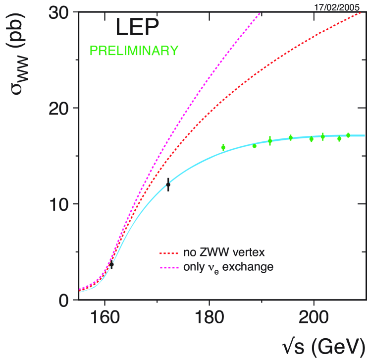
Figure 1.3: Cross section for the reaction $e+e−\rightarrow W+W−$ measured by the four LEP experiments, together with the full electroweak-theory simulation and cross sections that would result from $\nu$-exchange alone and from ($\nu+\gamma$)-exchange [20]

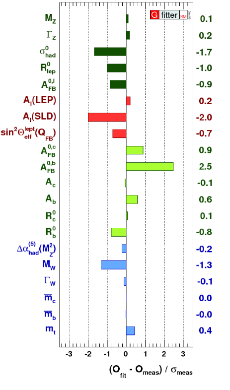
Figure 1.4: TPull values comparing Gfitter complete fit results with experimental determinations [21].

One of the striking features of the standard model is that it has withstood decades of increasingly intense experimental scrutiny. We briefly summerize the present experimental status of the SM.

Tree level: Historically, the electroweak theory was formulated in the context of extensive experimental information about the charged-current weak interactions (mainly from study of $\beta$ decay). The Fermi Theory of the weak charged current interactions had been developed and tested prior to the construction of the SM. The unitarity argument [19] made it clear that Fermi’s four-fermion description could not be valid above c.m. energy $\sqrt{s}\sim 600$ GeV. This necessitated the conjecture of heavy intermediate massive charged gauge bosons. The smallest unitary group which provides an off-diagonal generator (corresponding to the charged gauge boson) is SU(2). The relevant generators are $\tau^{1}$ and $\tau^{2}$. We further need a massless gauge boson to account for the infinite range electromagnetic interaction. Any association of photon with the neutral generator $\tau^{3}$ would lead to contradiction with respect to the charge assignment of particles. The gauge charges of fermions coupling to $W^{3}$ are $\pm{1\over 2}$, clearly different from the electric charges. Moreover, $W^{3}$ couples to neutrino, but photon does not. All in all, just with SU(2) gauge theory we cannot explain both weak and electromagnetic interactions. The next simplest construction is to avoid taking a simple group, but consider SU(2) $\times$ U(1). Further analysis of the reaction $\nu\bar{\nu}\to W^{+}W^{-}$ showed that the introduction of intermediate massive vector bosons, to make the weak interaction nonlocal, was non-renormalizable. However, with the advent of the Higgs mechanism, it was successfully moulded into the renormalizable theory discussed in the previous section, which allowed the calculation of radiative corrections.

The weak neutral current (WNC), along with the $W$ and $Z$, have been the primary predictions of the SM. The WNC was discovered in 1973 by the Gargamelle collaboration at CERN and by HPW at Fermilab. The structure of the WNC has been tested in many processes, including (purely weak) neutrino scattering $\nu e\rightarrow\nu e,\;\nu N\rightarrow\nu N,\;\nu N\rightarrow\nu X$; weak-electromagnetic interference in $e^{\pm}D\rightarrow eX$, atomic parity violation, and recently in polarized Möller scattering; and in $e^{+}e^{-}$ scattering above and below the $Z$ pole. The $W$ and $Z$ were discovered at CERN by the UA1 [16] and UA2 [17] groups in 1983 and the subsequent measurements of their masses have been in excellent agreement with the SM expectations (including the higher-order corrections [18]) discussed in the previous section. The cynosure of the LEP legacy is the triumphant verification of the gauge sector of the SM which involves the spontaneous breaking of the gauge group: $SU(2)_{L}\times U(1)_{Y}\rightarrow U(1)_{Q}$. Figure 1.4 obtained primarily from LEP II runs clearly verifies the SM gauge group. On one hand it clearly shows the existence of the $ZWW$ vertex confirming the non-abelian nature of the gauge group. Indirectly it also validates the idea of spontaneous symmetry breaking. To see this, note that the intermediate gauge bosons have to be massive to explain the $\beta$ decay data. However, explicit breaking leads to non-renormalizability. But the good behavior of the cross section with energy in Figure 1.4, indicates a renormalizable theory and thus implies spontaneous breaking of the gauge symmetry. In summary, this plot clearly indicates that the charged and neutral currents in the particle gauge interaction are in accordance with the SM prediction. This not only confirms the $SU(2)_{L}\times U(1)_{Y}$ gauge group but also demonstrates that it is spontaneously broken to $U(1)_{Q}$.

The $Z$ factories LEP and SLC allowed tests of the standard model at a precision of $\sim 10^{-3}$, much greater than what had previously been possible at high energies. In particular, the four LEP experiments ALEPH, DELPHI, L3, and OPAL at CERN produced some $2\times 10^{7}Z$’s at the $Z$-pole in the reactions $e^{+}e^{-}\rightarrow Z\rightarrow\ell^{+}\ell^{-}/q\bar{q}$. The SLD experiment at SLAC had a relatively smaller number of events, $\sim 5\times 10^{5}$, but had the significant advantage of the high polarization ($\sim$ 75%) of the $e^{-}$ beam. The $Z$ pole observables included the lineshape variables, $M_{Z},\Gamma_{Z},$ and $\sigma$; and the branching ratios into $e^{+}e^{-},\mu^{+}\mu^{-},\tau^{+}\tau^{-}$ as well as into $q\bar{q},c\bar{c},b\bar{b},$ and (less precisely) $s\bar{s}$. These could be combined to obtain the stringent constraint $N_{\nu}=2.9841\pm 0.0083$ on the number of ordinary neutrinos with $m_{\nu}<M_{Z}/2$ (i.e., on the number of families with a light neutrino). This gave the first experimental indication of the three generation flavor structure of the SM . At present, all the three pairs of quarks and leptons have been directly produced at collider experiments that give hard evidence for the three generation conjecture. This also constrained other invisible $Z$ decays.

The $Z$-pole experiments also measured a number of asymmetries, including forward-backward (FB), polarization, $\tau$ polarization, and mixed FB-polarization, which were especially useful in determining the weak angle $\theta_{W}$. The leptonic branching ratios and asymmetries confirmed the lepton family universality predicted by the SM. The result of fitting these observations with the SM predictions are generally in excellent agreement. Figure 1.4 shows the pull of the fittings in the SM. There is a hint of a tension between the lepton and quark asymmetries (most apparent in the $b$ quark forward-backward asymmetry $A_{fb}^{0,b}$ and the polarization asymmetry $A_{l}$.). This may well be a statistical fluctuation, but could possibly be suggesting new physics affecting the third family.

The recent activity in charged current interaction is centered around the study of the Cabibbo-Kobayashi-Maskawa (CKM) matrix which measures the mismatch between the family structure of the left-handed $u$-type and $d$-type quarks. For 3 families, $V_{CKM}$ involves three angles and one $CP$-violating phase after removing the unobservable $q_{L}$ phases as discussed before. There have been extensive recent studies, especially in $B$ and $K$ decays, to test the unitarity and consistency of $V_{CKM}$ as a probe of new physics and to test the origin of CP violation. A global fit [23], within the framework of the three-generation standard model, yields the following magnitudes $|{V_{ij}|}$ for the CKM matrix elements:

$${\left(\begin{array}[]{ccc}0.97419\pm 0.00022&0.2257\pm 0.0010&0.00359\pm 0.00016\\[4.0pt] 0.2256\pm 0.0010&0.97334\pm 0.00023&0.0415^{+0.0010}_{-0.0011}\\[4.0pt] 0.00874^{+0.00026}_{-0.00037}&0.0407\pm 0.0010&0.999133^{+0.000044}_{-0.000043}\end{array}\right).}$$ (1.38)

The present experimental status of the unitarity triangle is shown in Figure 1.5.

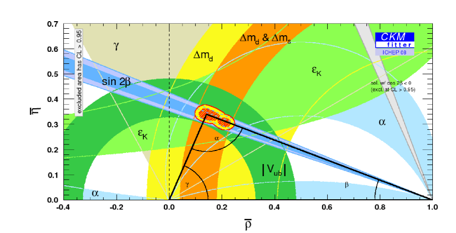
Figure 1.5: The unitarity triangle, showing overlap regions of several CP-conserving and CP-violating observables from the $K$ and $B$ systems. $\bar{\rho}$ and $\bar{\eta}$ are the same as $\rho$ and $\eta$ up to higher order corrections, and $\rho-i\eta=V_{ub}/(V_{cb}V_{us})$. Plot courtesy of the CKMfitter group [24], http://ckmfitter.in2p3.fr.

Higher order: The experimental probing of the SM has scrutinized it beyond the tree level. The present accuracy of experimental observations have enabled us to probe the quantum corrections of the theory. A brief discussion of this is in order, not only because it allows quantum verification of the SM, but also because it puts stringent constraints on any further extension of the theory. The discussion below closely follows the arguments laid out in [25]. Experimental measurements on the $Z$ pole at LEP has verified the radiative corrections to the gauge boson propagators to high precision. There are four two-point functions: $\Pi_{QQ}(q^{2}),\Pi_{Q3}(q^{2}),\Pi_{33}(q^{2}),\Pi_{11}(q^{2})$ where $Q\Rightarrow B_{\mu}$ and $(1,2,3)\Rightarrow(W_{\mu}^{1},W_{\mu}^{2},W_{\mu}^{3})$. Measurements have been made at two energy scales: $q^{2}=0,M_{Z}^{2}$. So there are eight two-point correlators. Of these eight, $\Pi_{\gamma\gamma}(0)=\Pi_{\gamma Z}(0)=0$ due to QED Ward identity. Three linear combinations can be absorbed in the redefinition of the parameters: $\alpha$, $G_{\mu}$ and $M_{Z}$. The remaining three independent combinations are called the Peskin-Takeuchi oblique electroweak parameters ($S$, $T$ and $U$). The parameters $T$ and $U$ capture the effects of custodial symmetry and weak isospin violation, while $S$ is a measure of weak isospin breaking alone [26]. Note that to cover all electroweak results, one needs to expand the number of such parameters, see [27] for further details. The definition of the parameters are given by,

$$\alpha T = \frac{\Pi_{WW}(0)}{M_{W}^{2}}-\frac{\Pi_{ZZ}(0)}{M_{Z}^{2}}$$ (1.39)

$$= \left(\frac{e^{2}}{(sin({\theta_{W}})cos({\theta_{W}}))^{2}}\right)\frac{1}{M_{Z}^{2}}\left(\Pi_{11}(0)-\Pi_{33}(0)\right)$$

and

$$S=\frac{16\pi}{M_{Z}^{2}}\left(\Pi_{33}(M_{Z}^{2})-\Pi_{33}(0)-\Pi_{3Q}(M_{Z}^{2})\right)$$ (1.40)

where $\Pi_{ab}(q)$ is the vacuum polarization amplitude with gauge bosons $a$ and $b$ in the external legs and the energy scale associated with the amplitude is ${q}$. A generic fermion-induced vacuum polarization diagram with gauge bosons in the two external lines has the following structure:

$$F^{\mu\nu}(m_{1},m_{2},\lambda,\lambda^{\prime})=(-)\int{d^{4}k\over(2\pi)^{4}}\frac{{\rm Tr}\left\{\gamma^{\mu}{1-\lambda\gamma_{5}\over 2}(\not{q}+\not{k}+m_{1})\gamma^{\nu}{1-\lambda^{\prime}\gamma_{5}\over 2}(\not{k}+m_{2})\right\}}{\{(q+k)^{2}-m_{1}^{2}\}(k^{2}-m_{2}^{2})}$$

$$=\frac{i}{16\pi^{2}}\int_{0}^{1}dx\left[\Delta-\ln\left\{\frac{-q^{2}x(1-x)+m_{1}^{2}x+m_{2}^{2}(1-x)}{\mu^{2}}\right\}\right]\left[2(1+\lambda\lambda^{\prime})x(1-x)(q_{\mu}q_{\nu}-q^{2}g_{\mu\nu})\right.$$

$$\left.~{}~{}~{}~{}+(1+\lambda\lambda^{\prime})(m_{1}^{2}x+m^{2}_{2}(1-x))g_{\mu\nu}-(1-\lambda\lambda^{\prime})m_{1}m_{2}g_{\mu\nu}\right]\,.$$ (1.41)

In the above equation, $m_{1}$ and $m_{2}$ are the masses of the fermions in the loop, and $\Delta(\equiv 2/(4-d)-\gamma+\ln 4\pi)$ is regularization scheme dependent divergent quantity. We are interested in the terms proportional to $g_{\mu\nu}$, the $\Pi$-functions are defined as $-i$ times these factors. By putting $\lambda=1$ and $\lambda^{\prime}=1$, we will get the left-left (LL) $\Pi$-function, given by

$$\Pi_{LL}(q^{2},m_{1}^{2},m_{2}^{2}) = -{1\over 4\pi^{2}}\int_{0}^{1}dx\left[\Delta+\ln{\mu^{2}\over-q^{2}x(1-x)+M^{2}(x)}\right]\left[q^{2}x(1-x)-{1\over 2}M^{2}(x)\right]$$

$$\mbox{where,}~{}~{}~{}~{}~{}~{}M^{2}(x)=m_{1}^{2}x+m_{2}^{2}(1-x).$$

Thus we find,

$$\Pi_{33}(q^{2}) = t^{2}_{3L}\Pi_{LL}(q^{2},m^{2},m^{2})$$ (1.43)

$$\Pi_{11}(q^{2}) = \frac{1}{2}\Pi_{LL}(q^{2},m_{1}^{2},m_{2}^{2}).$$ (1.44)

Now, supposing $m_{1}$ and $m_{2}$ are the masses of the two fermion states appearing in an SU(2) doublet, it immediately follows that

$$\Pi_{33}(q^{2}) = \frac{1}{4}\left[\Pi_{LL}(q^{2},m_{1}^{2},m_{1}^{2})+\Pi_{LL}(q^{2},m_{2}^{2},m_{2}^{2})\right]$$

$$\Pi_{11}(q^{2}) = \frac{1}{2}\Pi_{LL}(q^{2},m_{1}^{2},m_{2}^{2}).$$ (1.45)

One can now, in general, derive the SM prediction of the oblique parameters by using the above general scheme. For example the $T$ parameter is given by,

$$T={4\pi\over\sin^{2}\theta_{W}\cos^{2}\theta_{W}M_{Z}^{2}}\left[\Pi_{11}(0)-\Pi_{33}(0)\right].$$ (1.46)

The dominant effect of isospin violation indeed comes from top-bottom mass splitting, given by

$$T^{t-b}={4\pi\over\sin^{2}\theta_{W}\cos^{2}\theta_{W}M_{Z}^{2}}{N_{c}\over 32\pi^{2}}\left[{m_{t}^{2}+m_{b}^{2}\over 2}-{m_{t}^{2}m_{b}^{2}\over m_{t}^{2}-m_{b}^{2}}\ln{m_{t}^{2}\over m_{b}^{2}}\right]\simeq{1\over\pi}{m_{t}^{2}\over M_{Z}^{2}}.$$ (1.47)

In the last step, we have assumed that $m_{b}^{2}<<m_{t}^{2}$. Note that in the limit $m_{t}=m_{b}$, the contribution to $T$ vanishes, as expected. The contribution of the Higgs boson arises from $ZZh$ and $W^{+}W^{-}h$ interactions. It turns out that

$$\alpha T^{h}=-\frac{3G_{F}}{8\pi^{2}\sqrt{2}}(M_{Z}^{2}-M_{W}^{2})\ln\left(\frac{m_{h}^{2}}{M_{Z}^{2}}\right)\simeq-{\alpha\over 2\pi}\ln{m_{h}\over M_{Z}}.$$ (1.48)

Figure 1.6 shows the presently allowed region in the $S$-$T$ plane. Note that the SM contributions have been subtracted from the parameter, i.e. $S\rightarrow S^{exp}-S^{SM}$ and $T\rightarrow T^{exp}-T^{SM}$. The SM point on this plane would be the origin $(0,0)$ . Clearly this is in good agreement with experimental bounds and thus puts strong constraints on any further extension of the SM.

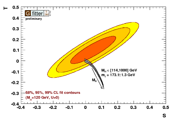
Figure 1.6: Contours of $68\%$, $95\%$, and $99\%$ CL in the TS-plane. The gray region shows the prediction within the SM. $M_{h}=120$ GeV and $m_{t}=173.2$ GeV defines the reference point at which all oblique parameters vanish. Plot courtesy Gfitter group [21].

1.1.2 Problems with the Standard Model

The SM is a mathematically-consistent renormalizable gauge field theory which is consistent with all experimental facts. It successfully predicted the existence and form of the weak neutral current, the existence and masses of the $W$ and $Z$ bosons, and the fermion family structure, as necessitated by the GIM mechanism. The charged current weak interactions and quantum electrodynamics are successfully incorporated into its folds. The consistency between theory and experiment indirectly tested the higher order corrections which established the ideas of renormalization in the context of the SM. When combined with quantum chromodynamics for the strong interactions, the standard model is almost certainly the approximately correct description of the elementary particles and their interactions down to at least $10^{-16}$cm $\sim 1$ TeV.

Despite its successes, the SM has a great deal of arbitrariness and fine-tuning [28], as is illustrated by the fact that it has 27 free parameters (29 if we consider the Majorana neutrinos), and that is not including electric charges. The parameters of the SM include: 3 gauge couplings; the $Z$ and Higgs masses; the QCD $\theta$ parameter; 12 fermion masses; 6 mixing and 2 CP phases (2 additional for Majorana $\nu$’s); and the cosmological constant. The Planck scale (Newton constant) is not included because only the ratios of mass parameters are observable. It is believed that this is a little too much for a fundamental theory of nature. The status of the laboratory/collider experiments in particle physics can best be summarized as: they are in good agreement with the SM predictions but there is still room for New Physics (NP) at the TeV or higher scale. At present there seems to be a $3.1\sigma$ discrepancy in the measurement of the anomalous magnetic moment of the muon ($(g-2)_{\mu}$)[30]. There are some tension in the field of b-physics as well. There is a $2\sigma$ discrepancy in the branching fraction of $D_{s}^{+}\rightarrow l^{+}\nu$ and a $2.5\sigma$ tension in the branching ratio of $B^{+}\rightarrow\tau^{+}\nu$. There are several other unexpected observations in b-physics that hint at the existence of NP at the TeV scale. In this regard the tension between the measured values of $(\sin 2\beta)_{\psi K_{s}}$ and $(\sin 2\beta)_{\phi K_{s}}$ , the large difference in the direct CP asymmetry $A_{CP}(B^{-}\rightarrow K^{-}\pi^{0})$ and $A_{CP}(\bar{B}^{0}\rightarrow K^{-}\pi^{+})$ etc are worth a mention. See [31] for a recent review of flavor physics.

The first hint of beyond SM physics came from the observed neutrino oscillations in solar neutrinos. This implied a non-zero mass for the neutrinos. Although the original Glashow-Wienberg-Salam formulation did not provide for massive neutrinos, they are however easily incorporated by the addition of right-handed states $\nu_{R}$ (Dirac mass) or as higher-dimensional operators, perhaps generated by an underlying seesaw (Majorana mass). The successful explanation of light neutrino masses is considered as a major outstanding issue with the SM. There are certain other severe deficiencies in the SM. Some of them are enumerated below.

Figure 1.7: Allowed Higgs mass as a function of top mass.

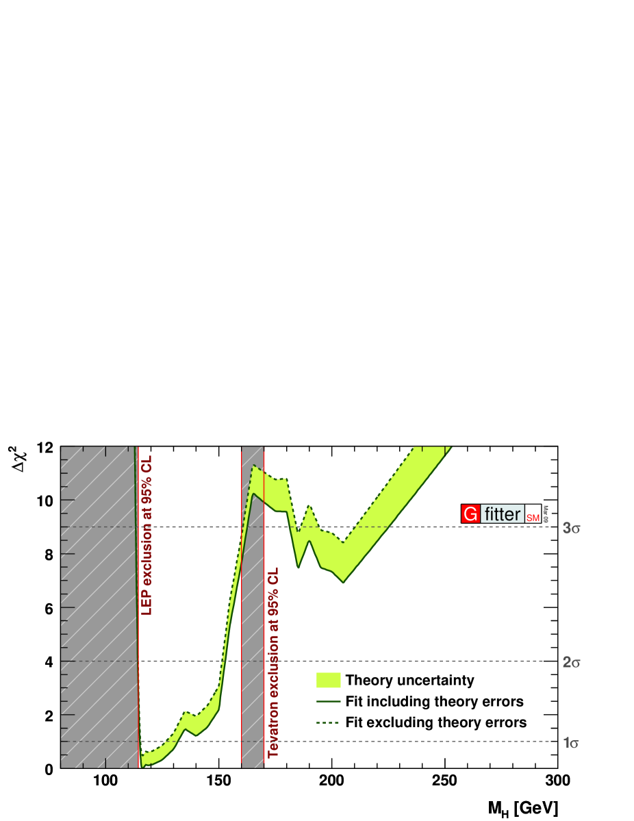
Figure 1.8: $\Delta\chi^{2}$ as a function of the Higgs-boson mass for the Gfitter complete fit, taking account of direct searches at LEP and the Tevatron. The solid (dashed) line gives the results when including (ignoring) theoretical errors. The minimum $\Delta\chi^{2}$ of the fit including theoretical errors is used for both curves to obtain the offset-corrected $\Delta\chi^{2}$ [21].

1. Cosmological consideration: The observed matter density of galaxies falls short of the measured matter as measured by the rotation curves. It is theorized that the baryon matter density is $\sim 4\%$. The rest of the universe is made up of $\sim 24\%$ dark matter and $\sim 72\%$ dark energy. In the last decade, the direct observation of gravitational lensing and observations in galactic collision[32] (in the ’Bullet’ cluster) events have provided hard evidence for the existence of Dark Matter (DM). The WMAP probe has measured the dark matter density to be between ($0.087<\Omega_{\rm DM}h^{2}<0.138$) [33] at $3\sigma$ range. SM neither provides any explanation for dark energy nor does it have a suitable dark matter candidate. Similarly, the observed asymmetry between matter and anti-matter in the universe quantified by $\eta\equiv\frac{n_{q}-n_{\bar{q}}}{n_{\gamma}}\simeq(6.1^{+.3}_{-.2})\times 10^{-10}$, cannot be explained within the framework of the SM. The minimum conditions needed to explain this asymmetry is enshrined in the Sakharov conditions, not fulfilled by the SM. For example, the baryon number (B), which should be broken to meet the Sakharov conditions, is an unbroken global symmetry of the SM. Further, the magnitude of the CP violation generated by the CKM picture in the SM is not sufficient to explain the baryon asymmetry in the universe.

2. Gauge Hierarchy problem: Quantum theories involving interacting elementary scalar fields are not natural. This has to do with the fact that the mass of an elementary scalar field is not associated with any approximate symmetry. Let us consider a self-interacting theory of a real scalar field:

   $${\cal L}_{scalar}=~{}{\frac{1}{2}~{}\partial^{\mu}\phi\partial_{\mu}\phi~{}-~{}{\frac{m^{2}}{2}}~{}\phi^{2}~{}-~{}{\frac{\lambda}{4!}}~{}\phi^{4}}$$ (1.49)

   and consider that it is coupled to a fermion by the following relation. We can write the Yukawa interaction Lagrangian as

   $$\mathcal{L}_{Y}=-h_{f}\phi\bar{f}_{L}f_{R}+~{}\mbox{h.c.}.$$ (1.50)

   where $f_{L,R}$ are the left and right chiral projection of the fermion $f$. After spontaneous symmetry breaking,

   $$\mathcal{L}_{Y}=-\frac{h_{f}}{\sqrt{2}}h\bar{f}_{L}f_{R}-\frac{h_{f}}{\sqrt{2}}v\bar{f}_{L}f_{R}+~{}\mbox{h.c.}$$ (1.51)

   The fermion mass is therefore given by $m_{f}=h_{f}{v\over{\sqrt{2}}}$.

   At the classical level, the limit mass $m\rightarrow 0$ does lead to scale invariance; but at quantum level scale symmetry is broken. Thus smallness of the scalar mass can not be protected against perturbative quantum corrections. In fact such corrections appear with quadratic divergences. Let us compute the two-point function with the zero momentum Higgs as the two external lines and fermions inside the loop. The corresponding diagram is in Figure 1.9[a].

   $$i\Pi^{f}_{hh}(0) = (-)\int\frac{d^{4}k}{(2\pi)^{4}}{\rm Tr}~{}\left[\left(-i\frac{h_{f}}{\sqrt{2}}\right)\frac{i}{\not{k}-m_{f}}\left(-i\frac{h_{f}}{\sqrt{2}}\right)\frac{i}{\not{k}-m_{f}}\right]$$ (1.52)

   $$= -2h_{f}^{2}\int\frac{d^{4}k}{(2\pi)^{4}}\left[\frac{1}{k^{2}-m_{f}^{2}}+\frac{2m_{f}^{2}}{(k^{2}-m_{f}^{2})^{2}}\right].$$

   The correction $\Delta m_{h}^{2}$ is proportional to $\Pi^{f}_{hh}(0)$. The first term in the RHS is quadratically divergent. The divergent correction to $m_{h}^{2}$ looks like

   $$\Delta m_{h}^{2}(f)=\frac{\Lambda^{2}}{16\pi^{2}}(-2h_{f}^{2})\,.$$ (1.53)

   Another divergent piece will appear from quartic Higgs vertex (i.e., $h^{4}$). The corresponding diagram is similar to what is displayed in Figure 1.9[c],

   $$\Delta m_{h}^{2}(h)=\frac{\Lambda^{2}}{16\pi^{2}}(\lambda)\,.$$ (1.54)

   We neglect the gauge boson contributions to the scalar self energy. Combining the above two divergent pieces, we obtain

   $$\Delta m_{h}^{2}=\frac{\Lambda^{2}}{16\pi^{2}}\left(-2h_{f}^{2}+\lambda\right).$$ (1.55)

   Figure 1.9: One-loop quantum corrections to the Higgs mass, due to a Dirac fermion $f$ [a], and scalars $\tilde{f}_{L,R}$ ([b] & [c]).

   This illustrates the typical quantum correction to scalar fields generated at one loop, that is quadratically divergent. The scalar sector of the SM faces a similar predicament. In this regard let us note the following points:

   • In the SM, the fermion masses are protected by the inexact chiral symmetry and the gauge boson masses are protected by the remnant gauge symmetry after spontaneous electroweak symmetry breaking, whereas, the Higgs field masses remain unprotected and receive quantum corrections that are quadratically dependent on the cut off. As discussed above, this is related to the inherent scale dependence of all fundamental scalar theories.

   • By itself, this is not a catastrophe, as one can envisage counter terms that will cancel such divergent quantum corrections. Unfortunately, the cut off of the SM is believed to be of the order of the Planck scale ($M_{pl}\sim 10^{19}$). Thus, to obtain a weak scale Higgs mass, one needs an unnatural cancellation between two uncorrelated numbers, i.e. the quantum correction and the counter term contribution. The situation gets uglier when it is noted that such cancellation has to take place order by order in the perturbation theory and there is no hope of convergence at any finite order.

   • It is also worthwhile to know that radiative corrections to the fermions or the gauge bosons are always proportional to their masses. Thus one cannot generate the masses of these fields purely from radiative contributions. This can be physically explained by noting that there is a mismatch in the degrees of freedom of a massive and massless gauge boson or fermion. The situation is completely different for the case of the fundamental scalars. Here one can generate the masses radiatively even if at tree level they are massless, as can be seen in Eq. 1.55. This is related to the fact that the $d.o.f.$ of a massive scalar field is identical to that of a massless scalar field.

   Thus we find the lack of symmetry protecting the Higgs mass and the large hierarchy between the weak scale and the Planck scale makes it difficult to explain light Higgs mass within the SM. This is known as the gauge hierarchy problem which is basically a naturalness issue with the SM.

   On the other hand, the other parameter of this theory, namely the $h^{4}$ coupling $\lambda$ is natural. This is so because, in the limit $\lambda\rightarrow 0$, we have a free scalar theory, which indeed has higher symmetry.

3. Gravity is not included: Gravity is not put on the same footing as other interactions in the SM. The vacuum energy $\langle V\rangle$ from electroweak symmetry breaking leads to an effective cosmological constant: $\Lambda_{\rm SSB}=8\pi G_{N}\langle V\rangle$ which is some $10^{50}$ times larger than the value of the cosmological constant, observed from the acceleration of the universe. Reconciliation with the observed value leads to extremely fine-tuned cancellation between the primordial value and the one generated dynamically by the electroweak symmetry breaking. There is no known accepted solution to the cosmological constant problem, but see [44] for an anthropically motivated fine-tuning associated with the string landscape.

Other than these severe shortcomings there are certain other criticism related to the SM viz., (a) The strong CP problem: The strong CP problem [46] refers to the fact that one can add the P, T, and CP-violating term $\frac{\theta}{32\pi^{2}}g_{s}^{2}F\tilde{F}$ to the QCD Lagrangian, where $\tilde{F}_{\mu\nu}=\epsilon_{\mu\nu\alpha\beta}F^{\alpha\beta}/2$ is the dual field and $\theta$ is an arbitrary dimensionless parameter. The experimental bound on the neutron electric dipole moment implies $\theta<10^{-9}$. One cannot simply set $\theta$ to zero because weak interaction corrections shift $\theta$ by $\delta\theta|_{\rm weak}\sim 10^{-3}$, again requiring a fine-tuned cancellation between the tree and weak contributions. (b) The fermion mass hierarchy problem: Beyond the ordinarily observed matter content that can be constituted by the following fermions $(\nu_{e},e^{-},u,d)$, the first family laboratory studies have confirmed the existence of $\geq 3$ families: $(\nu_{\mu},\mu^{-},c,s)$ and $(\nu_{\tau},\tau^{-},t,b)$ are heavier copies of the first family with no obvious explanation in the SM. The SM gives no prediction for the number of fermion generations. Furthermore, there is no explanation or prediction of their masses, which are observed to have hierarchical pattern spanning over 6 orders of magnitude between the top quark and the electron. Even more mysterious are the neutrinos, which are lighter still by many orders of magnitude. And (c)  The Gauge issue: The SM gauge group is complicated: it involves 3 distinct gauge couplings, of which only the electroweak part is parity-violating, and charge quantization (e.g., $|q_{e}|=|q_{p}|$) is put in by hand (anomaly cancellation by itself is not sufficient to determine all of the hypercharge assignments). The issue of charge quantization is important because it facilitates the electrical neutrality of atoms $(|q_{p}|=|q_{e}|)$. The complicated gauge structure suggests that there exists underlying unity in the interactions. This indicates the existence of superstring [35, 36, 37] or grand unified theory [38, 39, 40, 41, 42]. Charge quantization can also be explained in such classes of theories. Charge quantization may also be explained, at least in part, by the existence of magnetic monopoles [43] or the absence of anomalies.

It is worthwhile to note that the complete experimental verification of the SM has to wait the discovery of the hitherto elusive Higgs boson. Non-observation of the Higgs fields at the LEP II directly excludes Higgs mass below $114.4$ GeV, whereas the precision electroweak observables prefer a Higgs mass below $\sim 160$ GeV [29]. The major uncertainty in the electroweak fit of the Higgs mass comes from the uncertainty in the top quark mass. A plot of the values of the Higgs mass as a function of the top quark mass can be found in Figure 1.8. The $\Delta\chi^{2}$ plot for the global fitting of the Higgs mass can be found in Figure 1.8. The LHC is expected to discover the Higgs field though accurate measurement of its mass has to wait for future experiments, certainly the proposed International Linear Collider (ILC) will be able to do a better job in this regard.

1.2 Beyond the Standard Model

The above criticism of the SM provides a strong motivation for advocating theoretical constructions that extends the SM and solves some of it shortcomings. Most of the Beyond the Standard Model (BSM) physics [47] have been constructed to solve the gauge hierarchy problem. The models that have been discussed in the literarture may be categorized as follows:

1. Models with no fundamental scalars: Possibility to eliminate the elementary Higgs fields in favor of some dynamical symmetry breaking mechanism based on a new strong dynamics [48], e.g. technicolor, higher dimensional Higgs-less models. In technicolor, for example, the SSB is associated with the expectation value of a fermion bilinear, analogous to the breaking of chiral symmetry in QCD. Extended technicolor, top-color, and composite Higgs models all fall into this class. Higher dimensional Higgs less models [52]) use the boundary conditions in the extra dimensions to break the electroweak symmetry.

2. Models that invoke symmetry to protect Higgs mass: e.g. supersymmetry, gauge-Higgs unified models, little Higgs. In supersymmetry [54], the quadratically-divergent contributions of fermion and boson loops cancel, leaving only much smaller effects of the order of supersymmetry-breaking. There are also (non-supersymmetric) extended models in which the cancellations are between bosons or between fermions. This class includes Little Higgs models [49, 50], in which the Higgs is forced to be lighter than new TeV scale dynamics because it is a pseudo-Goldstone boson of an approximate underlying global symmetry, and Twin-Higgs models [51].

3. Models that try to bridge the gap between the two scales of the Standard Model:
   e.g. ADD - large extra dimension, RS - warped extra dimension. In these models space-time geometry is used to relate $M_{pl}$ and a much lower fundamental scale, by providing a cutoff at the inverse of the extra dimension scale. See  [55, 56] for further details.

1.3 Supersymmetry

Figure 1.10: The running Gauge coupling unification within the framework of MSSM [59].

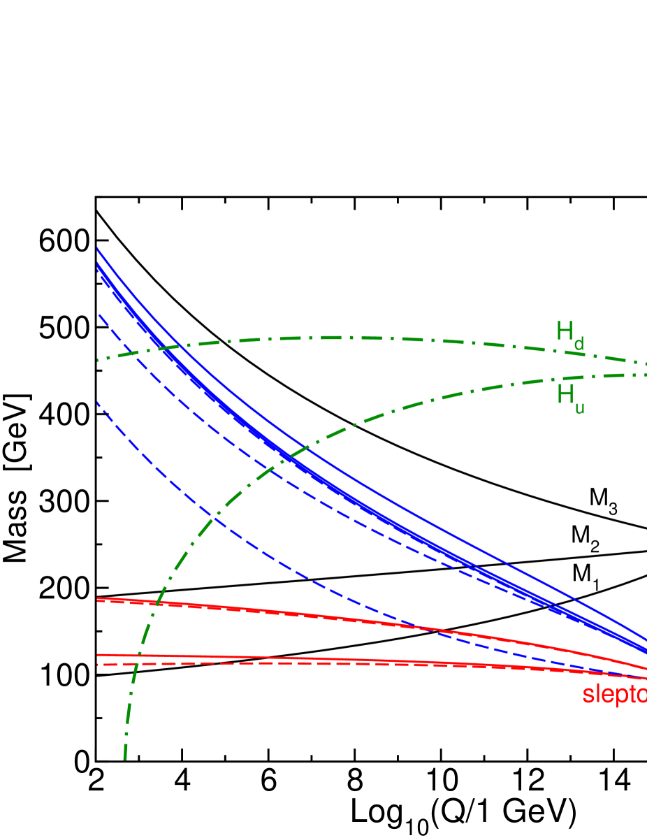
Figure 1.11: The renormalization group running of soft parameters in mSUGRA. Negative $m_{H_{u}^{2}}$ in low energy triggers EWSB [54].

Let us tweak the analysis we did to reach Eq 1.55. Consider that the scalar inside the loop in Figure 1.9 [c] is not $\phi$ but some different scalar field $\tilde{f_{L}}/\tilde{f_{R}}$, where the coupling is $\sim\lambda\phi^{2}\tilde{f}_{L/R}^{2}$. Note that if there are two such scalars ($\tilde{f}_{L}$ and $\tilde{f}_{R}$), the Eq. 1.55 becomes,

$$\Delta m_{h}^{2}=\frac{2\Lambda^{2}}{16\pi^{2}}\left(-h_{f}^{2}+\lambda\right).$$ (1.56)

We find that the entire quadratic divergence piece in the quantum correction to the scalar mass vanishes if,

$$h_{f}^{2}=\lambda.$$ (1.57)

There are pairwise cancellations between fermionic contributions and the contributions from a pair of scalars. Apriori, such relations between the coupling of two fields are unnatural. Supersymmetry is a space-time symmetry which relates the bosonic degrees of freedom to the fermionic degrees of freedom [57, 54, 58], and thus can justify relations like the one expressed in Eq. 1.57.

Supersymmetry (SUSY) is the most popular extension of the SM because it provides a very aesthetic way to address the gauge hierarchy problem and ameliorate various other shortcomings of the SM. Owing to its overwhelming popularity in the parlays of particle physics, a brief discussion of SUSY is now in order. Some of the attractive features of the SUSY models are:

1. Supersymmetry solves the gauge hierarchy problem : As discussed, the quantum corrections to the Higgs mass from a bosonic loop and a fermionic loop have opposite signs. So if the couplings are identical and boson is mass degenerate with the fermion, the net contribution would cancel! Supersymmetry fits this bill very well, as for every particle, supersymmetry provides a mass degenerate partner differing by spin $1\over 2$ and having identical couplings.

2. Supersymmetry leads to unification of gauge couplings: In the SM, when the gauge couplings are extrapolated to high scale from their measured values at the weak scale, they come close to each other but do not meet at a single point. In supersymmetry, the running gauge couplings do meet at a point  [59], at the scale $M_{\rm GUT}\sim 2\times 10^{16}$ GeV, provided the superparticles weigh around 1 TeV, see Figure 1.11.

3. Supersymmetry triggers EWSB: To drive spontaneous symmetry breaking in SM, one requires to set the scalar mass in the Lagrangian, to a negative value by hand. In SUSY theories, the square of one of the Higgs mass $m_{H_{u}}^{2}$, can be made negative by radiative correction. In the Minimal Supersymmetric Standards Model (MSSM) that we shall discuss later, one can start with a positive value of the Higgs mass at the gauge coupling unification ($M_{\rm GUT}$) scale. The running of the parameters drives the $m_{H_{u}}^{2}$ to a negative value at the weak scale driving electroweak symmetry breaking, see Figure 1.11. In MSSM it is the heavy top quark contribution to the radiative correction that induces the sign flip.

4. Supersymmetry provides a cold dark matter candidate: Supersymmetry with conserved $R$-parity can provide a dark matter candidate. The lightest supersymmetric particle (LSP) cannot decay due to the $R$-parity that forbids vertices with odd number of super-partners of the SM fields. Thus the LSP is a stable particle and a viable cold dark matter candidate.

5. Supersymmetry provides a framework to turn on gravity: As discussed earlier, SM do not provide a framework to unify gravity with the other particle interactions. But SUSY does better in this regard. Space-time transformations are naturally included in the SUSY transformations. Local supersymmetry leads to supergravity that gives a gateway to include gravity in a quantum field theoretic famework. Most string models invariably include supersymmetry as an integral part.

1.3.1 SUSY algebra

Supersymmetry is a general space-time symmetry that is allowed by the Poincare algebra. Unlike the Lorentz transformations supersummetric transformations are mediated by fermionic charges. A supersymmetry transformation turns a bosonic state into a fermionic state, and vice versa. The operator $Q$ that generates such transformations must be an anti-commuting spinor, generating the following transformations,

$$Q|{\rm Boson}\rangle=|{\rm Fermion}\rangle,\qquad\qquad Q|{\rm Fermion}\rangle=|{\rm Boson}\rangle.$$ (1.58)

Spinors are intrinsically complex objects, so $Q^{\dagger}$ (the hermitian conjugate of $Q$) is also a symmetry generator. Note that in general there can be arbitrary number of such generator pairs ($Q_{i}\&Q_{i}^{\dagger}$) that can simultaneously generate SUSY transformations. The number of such generators are going to be represented by $N$. Increase in $N$ generally results in more symmetric and therefore more constrained theories. In this chapter we will stick to the $N=1$ version of the theory. The possible forms for such symmetries in a quantum field theory are highly restricted by the no go theorem put forward by Haag-Lopuszanski-Sohnius, which is basically an extension of the Coleman-Mandula theorem [60]. The basic result of this theorem is, that space-time symmetry transformations by generators of spin greater than 1 is prohibited.

Generic supersymmetric charges satisfy the algebra of anti-commutation and commutation relations with the schematic form

$$\{Q,Q^{\dagger}\}=P^{\mu},$$ (1.59)

$$\{Q,Q\}=\{Q^{\dagger},Q^{\dagger}\}=0,$$ (1.60)

$$[P^{\mu},Q]=[P^{\mu},Q^{\dagger}]=0,$$ (1.61)

where $P^{\mu}$ is the four-momentum generator of space-time translations. Here we have suppressed the spinorial index. Note that the appearance of $P^{\mu}$ on the right-hand side of Eq. 1.59 is understandable, since it transforms under Lorentz boosts and rotations as a spin-1 object while $Q$ and $Q^{\dagger}$ on the left-hand side, each transforms as a spin-1/2 object. This natural appearance of the generator for space-time translation provides a handle to incorporate gravity in SUSY theories.

The single-particle states of a supersymmetric theory fall into irreducible representations of the supersymmetry algebra, called supermultiplets. Each supermultiplet contains both fermionic and bosonic states, which are called superpartners of each other. If $|\Omega\rangle$ and $|\Omega^{\prime}\rangle$ are members of the same supermultiplet, then the $|\Omega^{\prime}\rangle$ can be obtained by operating some combination of $Q$ and ${Q}^{\dagger}$ operators on $|\Omega\rangle$, up to a space-time translation or rotation. The squared mass operator $-P^{2}$ commutes with the operators $Q$, ${Q}^{\dagger}$, and with all space-time rotation and translation operators. It follows immediately that members of the same supermultiplet will have equal mass eigenvalues i.e they will be mass degenerate. The supersymmetry generators $Q,Q^{\dagger}$ also commute with all internal symmetry generators in general and the generators of gauge transformations in particular. Therefore particles in the same supermultiplet must also be in the same representation of the gauge group, i.e. same electric charges, weak isospin, color degrees of freedom etc.

Each supermultiplet contains an equal number of fermionic and bosonic degrees of freedom. This can be demonstrated easily. Consider the operator $(-1)^{2s}$ where $s$ is the spin angular momentum. By the spin-statistics theorem, this operator has eigenvalue $+1$ acting on a bosonic state and eigenvalue $-1$ acting on a fermionic state. Any fermionic operator will turn a bosonic state into a fermionic state and so on. Therefore $(-1)^{2s}$ must anti-commute with every fermionic operator in the theory, and in particular with $Q$ and $Q^{\dagger}$. Now, within a given supermultiplet, consider the subspace of states $|i\rangle$ with the same eigenvalue $p^{\mu}$ of the four-momentum operator $P^{\mu}$. In view of Eq. 1.61, any combination of $Q$ or $Q^{\dagger}$ acting on $|i\rangle$ must give another state $|i^{\prime}\rangle$ with the same four-momentum eigenvalue. Therefore one has a completeness relation $\sum_{i}|i\rangle\langle i|=1$ within this subspace of states. Now one can take a trace over all such states of the operator $(-1)^{2s}P^{\mu}$ (including each spin helicity state separately):

$$\sum_{i}\langle i|(-1)^{2s}P^{\mu}|i\rangle = \sum_{i}\langle i|(-1)^{2s}QQ^{\dagger}|i\rangle+\sum_{i}\langle i|(-1)^{2s}Q^{\dagger}Q|i\rangle$$ (1.62)

$$= \sum_{i}\langle i|(-1)^{2s}QQ^{\dagger}|i\rangle+\sum_{i}\sum_{j}\langle i|(-1)^{2s}Q^{\dagger}|j\rangle\langle j|Q|i\rangle\qquad{}$$

$$= \sum_{i}\langle i|(-1)^{2s}QQ^{\dagger}|i\rangle+\sum_{j}\langle j|Q(-1)^{2s}Q^{\dagger}|j\rangle$$

$$= \sum_{i}\langle i|(-1)^{2s}QQ^{\dagger}|i\rangle-\sum_{j}\langle j|(-1)^{2s}QQ^{\dagger}|j\rangle$$

$$= 0.$$

The first equality follows from the supersymmetry algebra relation Eq. 1.59; the second and third from use of the completeness relation; and the fourth from the fact that $(-1)^{2s}$ must anti-commute with $Q$. Now $\sum_{i}\langle i|(-1)^{2s}P^{\mu}|i\rangle=\,p^{\mu}$ Tr[$(-1)^{2s}$] is just proportional to the number of bosonic degrees of freedom $n_{B}$ minus the number of fermionic degrees of freedom $n_{F}$ in the trace, so that

$$n_{B}=n_{F}$$ (1.63)

must hold for a given $p^{\mu}\neq 0$ in each supermultiplet.

The simplest possibility for a supermultiplet consistent with Eq. 1.63 has a single Weyl fermion (with two spin helicity states, so $n_{F}=2$) and two real scalars (each with $n_{B}=1$). It is natural to assemble the two real scalar degrees of freedom into a complex scalar field. This combination of a two-component Weyl fermion and a complex scalar field is called a chiral supermultiplet.

Another possibility for a supermultiplet contains a spin-1 vector boson. If the theory is to be renormalizable, this must be a gauge boson that is massless, at least before the gauge symmetry is spontaneously broken. A massless spin-1 boson has two helicity states, so the number of bosonic degrees of freedom is $n_{B}=2$. Its superpartner is therefore a massless spin-1/2 Weyl fermion, again with two helicity states, so $n_{F}=2$. Gauge bosons transform in the adjoint representation of the gauge group, so their fermionic superpartners, called gauginos, must also follow suit. Since the adjoint representation of a gauge group is self conjugate, the gaugino fermions must have the same gauge transformation properties for left-handed and for right-handed components. Such a combination of spin-1/2 gauginos and spin-1 gauge bosons is called a vector supermultiplet.

1.3.2 The generic SUSY Lagrangian

Before zooming into the supersymmetric extension of the standard model we review the generic features of a SUSY Lagrangian.

Consider a massless and therefore two-component Weyl fermion, $\psi$ whose superpartner is a complex scalar $\phi.$ Both have two real degrees of freedom. However in the off-shell condition, the fermion is a four-component field with four degrees of freedom, and we want supersymmetry to hold for the full field theory. So we introduce an additional complex scalar $F$ to match the off-shell degrees of freedom. $F$ is called an auxiliary field and has no physical particle interpretation. A complete chiral superfield will thus contain the fields $(\psi,\phi,F)$. The Lagrangian can be written as

$$-\mathcal{L}_{chiral}=\sum_{i}(\partial^{\mu}\phi_{i}^{\ast}\partial_{\mu}\phi_{i}+\bar{\psi}_{i}\gamma^{\mu}\partial_{\mu}\psi_{i}+F_{i}^{\ast}F_{i}).$$ (1.64)

The sum is over all chiral supermultiplets in the theory. Note that the dimensions of $F$ are $[F]=m^{2}.$ The Euler-Lagrange equations of motion for $F$ are $F=F^{\ast}=0,$ signifying the fact that they are not physical fields. The supersymmetry transformations defined above are so that $\mathcal{L}_{chiral}$ is invariant. Next we write the most general set of renormalizable interactions,

$$\mathcal{L}_{int}=-\frac{1}{2}W^{ij}\psi_{i}\psi_{j}+W^{i}F_{i}+c.c.$$ (1.65)

where $W^{ij}$ and $W^{i}$ are functions of only the scalar fields (i.e. $\phi_{i}$’s in our context), and $W^{ij}$ is symmetric. If they depend on the fermion or auxiliary fields the associated terms would have dimension greater than four, and therefore would become non-renormalizable.

The SUSY transformations mix fermions and bosons, $\phi\rightarrow\phi+\varepsilon\psi,\psi\rightarrow\psi+\varepsilon\phi$. Here $\varepsilon$ must be a spinor so each term behaves the same way in spin space, and we can take $\varepsilon$ to be a constant spinor in space-time, and infinitesimal, which corresponds to a global SUSY transformation. Then the variation of the Lagrangian (which must vanish or change only by a total derivative if the theory is invariant under the supersymmetry transformation) contains two terms with four spinors:

$$\delta\mathcal{L}_{int}=-\frac{1}{2}\frac{\delta W^{ij}}{\delta\phi_{k}}(\varepsilon\psi_{k})\psi_{i}\psi_{j}-\frac{1}{2}\frac{\delta W^{ij}}{\delta\phi_{k}^{\ast}}(\varepsilon^{\dagger}\psi_{k}^{\dagger})\psi_{i}\psi_{j}+c.c.$$ (1.66)

Neither term can cancel against some other term. For the first term there is a Fierz identity $(\varepsilon\psi_{i})(\psi_{j}\psi_{k})+(\varepsilon\psi_{j})(\psi_{k}\psi_{i})+(\varepsilon\psi_{k})(\psi_{i}\psi_{j})=0$, so if and only if $\delta W^{ij}/\delta\phi_{k}$ is totally symmetric under interchange of i, j and k, the first term vanishes identically. For the second term, the presence of the hermitian conjugation allows no similar identity, so it must vanish explicitly, which implies $\delta W^{ij}/\delta\phi_{k}^{\ast}=0,$and thus $W^{ij}$ cannot depend on $\phi^{\ast}$! $W^{ij}$ must be an analytic function of the complex field $\phi.$ Therefore we can write

$$W^{ij}=M^{ij}+y^{ijk}\phi_{k},$$ (1.67)

where $M^{ij}$ is a symmetric matrix that will be the fermion mass matrix, and $y^{ijk}$ can be called general SUSY version of the SM Yukawa couplings. Then it is very convenient to define

$$W_{super}=\frac{1}{2}M^{ij}\phi_{i}\phi_{j}+\frac{1}{6}y^{ijk}\phi_{i}\phi_{j}\phi_{k}$$ (1.68)

and $W^{ij}=\delta^{2}W/\delta\phi_{i}\delta\phi_{j}.$ $W_{super}$ is the superpotential, an analytic function of $\phi$, and a central function of the formulation of the theory. $W$ is by construction, gauge invariant and Lorentz invariant, and an analytic function of $\phi$ (i.e. it cannot depend explicitly on $\phi^{\ast}$), so it is highly constrained. It determines the most general non-gauge interactions of the chiral superfields.

A similar argument for the parts of $\delta\mathcal{L}_{int}$ which contains a spacetime derivative implies that $W^{i}$ is determined in terms of $W$ as well,

$$W^{i}=\frac{\delta W}{\delta\phi_{i}}=M^{ij}\phi_{j}+\frac{1}{2}y^{ijk}\phi_{j}\phi_{k}.$$ (1.69)

Because of the interaction terms, the equations of motion for $F$ becomes non-trivial, and are now modified to,

$$F_{i}=-W_{i}^{\ast}.$$ (1.70)

The potential for the scalar fields of the theory is now given by,

$$V=\sum_{i}\left|F_{i}\right|^{2}.$$ (1.71)

This part of the scalar potential is called the “F-term” contribution, and is automatically bounded from below, an important feature of SUSY theories.

Now consider massless gauge bosons, like photons, $A_{\mu}^{a},$ with gauge index $a,$ and two degrees of freedom. Their superpartners are two-component spinors $\lambda^{a}.$ As stated earlier, the off shell fermion has four degrees of freedom, while the an off shell boson has three, the two transverse polarizations and a longitudinal polarization. So again it is necessary to add an auxiliary field, a real one since only one degree of freedom is needed, called $D^{a}.$ Then the complete Lagrangian has additional pieces

$$\mathcal{L}_{gauge}=-\frac{1}{4}F_{\mu\nu}^{a}F_{a}^{\mu\nu}-i\lambda^{\dagger a}\gamma^{\mu}D_{\mu}\lambda^{a}+\frac{1}{2}D^{a}D^{a},$$ (1.72)

where, as usual,

$$F_{\mu\nu}^{a}=\partial_{\mu}A_{\nu}^{a}-\partial_{\nu}A_{\mu}^{a}-gf^{abc}A_{\mu}^{b}A_{\nu}^{c},$$ (1.73)

and the covariant derivative is

$$D_{\mu}\lambda^{a}=\partial_{\mu}\lambda^{a}-gf^{abc}A_{\mu}^{b}\lambda^{c}.$$ (1.74)

It is crucial for gauge invariance that the same coupling $g$ appears in the definition of the tensor $F_{\mu\nu}$ and in the covariant derivative.

If we couple the chiral superfield with the vector superfields we must replace all the derivatives in Eq. 1.64 by the corresponding covariant derivatives. There are additional gauge invariant term to be added to the Lagrangian beyond the ones discussed above given by,$(\phi_{i}^{\ast}T^{a}\phi_{i})D^{a}$ and $\lambda^{\dagger a}(\psi^{\dagger}T^{a}\phi),$ and its conjugate, with an arbitrary dimensionless coefficient. Requiring the entire Lagrangian to be invariant under supersymmetry transformations determines the arbitrary coefficient and gives the final a resulting Lagrangian

$$\mathcal{L}=\mathcal{L}_{gauge}+\mathcal{L}^{cov}_{chiral}+g_{a}(\phi^{\ast}T^{a}\phi)D^{a}-\sqrt{2}g_{a}[(\phi^{\ast}T^{a}\psi)\lambda^{a}+\lambda^{\dagger a}(\psi^{\dagger}T^{a}\phi)]$$ (1.75)

where all derivatives in earlier forms are replaced by covariant ones. Note that the requirement of supersymmetry requires that the couplings in the last two terms be gauge couplings, even though they are not normal gauge interactions! The chiral part of the Lagrangian $\mathcal{L}_{chiral}$ can be explicitly written as,

$$\mathcal{L}_{chiral} = D^{\mu}\phi_{i}^{\ast}D_{\mu}\phi_{i}+\bar{\psi}_{i}\gamma^{\mu}D_{\mu}\psi_{i}$$ (1.76)

$$+ (\frac{1}{2}M_{ij}\psi_{i}\psi_{j}+\frac{1}{2}y^{ijk}\phi_{i}\psi_{j}\psi_{k}+c.c.)+F_{i}^{\ast}F_{i}.$$

The equations of motion for $D^{a}$ give $D^{a}=-g(\phi^{\ast}T^{a}\phi),$ so the expanded scalar potential is now given by

$$V=F^{\ast i}F_{i}+\frac{1}{2}\sum_{a}D^{a}D^{a}=\left|\partial W/\partial\phi_{i}\right|^{2}+\frac{1}{2}\sum_{a}g_{a}^{2}(\phi^{\ast}T^{a}\phi)^{2},$$ (1.77)

the sum is over $a=1,2,3$ for the three gauge couplings. The two terms are called F-terms and D-terms. Note that even now the scalar potential is bounded from below .

1.3.3 The Minimal Supersymmetric Standard Model

Names		spin 0	spin 1/2	$SU(3)_{C},\,SU(2)_{L},\,U(1)_{Y}$
squarks, quarks	$Q$	$({\widetilde{u}}_{L}\>\>\>{\widetilde{d}}_{L})$	$(u_{L}\>\>\>d_{L})$	$(\>{3},\>{2}\>,\>{1\over 6})$
	$\overline{u}$	${\widetilde{u}}^{*}_{R}$	$u^{\dagger}_{R}$	$(\>{\overline{3}},\>{1},\>-{2\over 3})$
	$\overline{d}$	${\widetilde{d}}^{*}_{R}$	$d^{\dagger}_{R}$	$(\>{\overline{3}},\>{1},\>{1\over 3})$
sleptons, leptons	$L$	$({\widetilde{\nu}}\>\>{\widetilde{e}}_{L})$	$(\nu\>\>\>e_{L})$	$(\>{1},\>{2}\>,\>-{1\over 2})$
	$\overline{e}$	${\widetilde{e}}^{*}_{R}$	$e^{\dagger}_{R}$	$(\>{1},\>{1},\>1)$
Higgs, Higgsinos	$H_{1}$	$(H_{1}^{+}\>\>\>H_{1}^{0})$	$(\widetilde{H}_{1}^{+}\>\>\>\widetilde{H}_{1}^{0})$	$(\>{1},\>{2}\>,\>+{1\over 2})$
	$H_{2}$	$(H_{2}^{0}\>\>\>H_{2}^{-})$	$(\widetilde{H}_{2}^{0}\>\>\>\widetilde{H}_{2}^{-})$	$(\>{1},\>{2}\>,\>-{1\over 2})$
		spin 1/2	spin 1
gluino, gluon		$\widetilde{g}$	$g$	$(8,1,0)$
winos, W-bosons		$\widetilde{W}^{\pm}$, $\widetilde{W}^{0}$	${W^{\pm}}$, ${W^{0}}$	$(1,3,0)$
bino, B-boson		$\widetilde{B}^{0}$	${B^{0}}$	$(1,1,0)$

Table 1.1: Supersymmetric partners with the Standard Model members

The MSSM is the minimal SUSY extension of the SM. The field content includes the SM particles and their superpartners as can be seen in Table 1.1. All of the quarks and leptons are put in chiral superfields with their superpartners (squarks and sleptons respectively). In Table 1.1 all superpartners are denoted with a tilde, and there is a superpartner for each chiral state of each SM fermion. This enables us to treat fermions of different chirality differently. The gauge bosons are put in vector superfields with their fermionic superpartners (the gauginos). Since $W$ is analytic in the scalar fields, we cannot include the complex conjugate of the scalar field as in the SM to give mass to the down quarks, so there must be a minimum of two Higgs doublets in supersymmetric theories, and each has its own superpartner (the Higgsinos). The requirement that the trace anomalies vanish so that the theories stay renormalizable, $TR(Y^{3})=TR(T_{3L}^{2}Y)=0$, also implies the existence of even number of Higgs doublets.

The Kinetic terms of these fields are direct generalization of Eq. 1.75. What remains to be specified is the superpotential. This is given by,

$$W=\bar{u}Y_{u}QH_{u}-\bar{d}Y_{d}QH_{d}-\bar{e}Y_{e}LH_{d}+\mu H_{u}H_{d}.$$ (1.78)

All the fields are chiral superfields. The bars over $u,d,e$ are in the sense, that right chiral fields are written as left conjugates and has nothing to do with non-analyticity. The sign convention is designed to generate positive masses. The generational and fermionic indices have been suppressed. For example the fourth term with the fermionic index would read like $\bar{u}_{ai}(Y_{u})_{ij}Q_{j\alpha}^{a}(H_{u})_{\beta}\varepsilon_{\alpha\beta}$

The Yukawa couplings $Y_{u}$ etc. are dimensionless 3$\times 3$ family matrices that determine the masses of quarks and leptons, and the angles and phase of the CKM matrix after $H_{u}^{0}$ and $H_{d}^{0}$ get vevs. They also contribute to the squark-quark-Higgsino couplings etc. This is the most general superpotential for the MSSM if we assume baryon and lepton number are conserved.

R parity:Within the SM, B and L are accidental global symmetries of the Lagrangian. Thus B and L violating interactions are absent.These additional terms could be incorporated in $W$ keeping it analytic, gauge invariant, and Lorentz invariant, but violating baryon and/or lepton number conservation. These terms are,

$$W_{R}=\lambda_{ijk}L_{i}L_{j}\bar{e}_{k}+\lambda_{ijk}^{\prime}L_{i}Q_{j}\bar{d}_{k}+\lambda_{ijk}^{\prime\prime}\bar{u}_{i}\bar{d}_{j}\bar{d}_{k}+\mu^{\prime i}L_{i}H_{u}.$$ (1.79)

The couplings $\lambda,\lambda^{\prime},\lambda^{\prime\prime}$ are matrices in the family space. Combination of the second and third terms in Eq 1.79 lead to rapid proton decay. This requires extreme suppression of either or both terms which again brings in the naturalness problem into the theory. Rather, B and L conservation consistent with observation should arise naturally from the symmetries of the theory. This is dealt with by imposing a symmetry like the R-parity or a variant called the matter parity, on the Lagrangian. The R parity is defined as,

$$R=(-1)^{3(B-L)+2S}$$ (1.80)

where $S$ is the spin. Then SM particles and Higgs fields are even, superpartners odd. This is a discrete $\mathbb{Z}_{2}$ symmetry. Equivalently, one can use “matter parity”,

$$P_{m}=(-1)^{3(B-L)}.$$ (1.81)

It is now conjectured that a term in $W$ is only allowed if $P_{m}=+1.$ Gauge fields and Higgs are assigned $P_{m}=+1,$ and quark and lepton supermultiplets $P_{m}=-1.$ $P_{m}$ commutes with supersymmetry and forbids $W_{R}.$ Matter parity could be an exact symmetry, and such symmetries do arise in string theory. If R-parity or matter parity holds, there are major phenomenological consequences,

• At colliders, or in loops, superpartners are produced in pairs.

• Each superpartner decays into one other superpartner (or an odd number).

• The lightest superpartner (LSP) is stable. That determines supersymmetry collider signatures, and makes the LSP a good candidate for the cold dark matter of the universe.

The Soft breaking of MSSM: Unfortunately the simple SUSY extension of the standard model do not work. Supersymmetry predicts mass degenerate superpartners of the SM fields, the failure to observe these in experiments spells the doom for exact supersymmetric theory. The alternative is to break supersymmetry in a way that will predict a mass difference between the SM particles and their superpartners but will preserve the correlation in their coupling that is crucial for cancellation of the quadratically divergent quantum correction to the scalar masses. This is known as soft supersymmetry breaking.

Supersymmetry breaking can be driven spontaneously. To see this let us write down the general SUSY Hamiltonian using Eq. 1.59-1.61,

$$H=P^{0}={1\over 4}(Q_{1}Q_{{1}}^{\dagger}+Q_{{1}}^{\dagger}Q_{1}+Q_{2}Q_{{2}}^{\dagger}+Q_{{2}}^{\dagger}Q_{2}).$$ (1.82)

The vacuum not respecting supersymmetry translates into the conditions: $Q|0\rangle\neq 0$ and $Q^{\dagger}|0\rangle\neq 0$. When these conditions are imposed on Eq. 1.82 we find that it implies: $\langle 0|H|0\rangle>0$. In most general cases $\langle 0|H|0\rangle\equiv\langle 0|V|0\rangle$. Referring to the definition of the potential $V$ given in Eq. 1.77, the condition for spontaneous supersymmetry breaking can be realized if either of the auxiliary fields ($F\mbox{or}D$) develop a non-zero vev. This simple picture of spontaneous breaking of supersymmetry cannot be implimented in the MSSM with the field content defined in Table 1.1. Further, spontaneous symmetry breaking generally implies certain mass sum rules that put all spontaneously broken supersymmetric extension of the SM at variance with experimental observations.

Though it is conjectured that supersymmetry is broken spontaneously, possibly in some hidden sector, the pragmatic approach is to parametrize this ignorance into certain phenomenological parameters. This constitutes the soft breaking Lagrangian of the theory. For the MSSM we have,

$$-\mathcal{L}_{soft} =\frac{1}{2}(M_{3}\tilde{g}\tilde{g}+M_{2}\widetilde{W}\widetilde{W}+M_{1}\widetilde{B}\widetilde{B}+c.c.)$$

$$\hskip 57.81621pt+\widetilde{Q}^{{\dagger}}m_{Q}^{2}\widetilde{Q}+\widetilde{\bar{u}}^{{\dagger}}m_{\bar{u}}^{2}\widetilde{\bar{u}}+\widetilde{\bar{d}}^{{\dagger}}m_{d}^{2}\widetilde{\bar{d}}+\widetilde{L}^{{\dagger}}m_{L}^{2}\widetilde{L}+\widetilde{\bar{e}}^{{\dagger}}m_{\bar{e}}^{2}\widetilde{\bar{e}}$$

$$\hskip 36.135pt+(\widetilde{\bar{u}}a_{u}\widetilde{Q}H_{u}-\widetilde{\bar{d}}a_{d}\widetilde{Q}H_{d}-\widetilde{\bar{e}}a_{e}\widetilde{L}H_{d}+c.c.)$$

$$\hskip 36.135pt+m_{H_{u}}^{2}H_{u}^{\ast}H_{u}+m_{H_{d}}^{2}H_{d}^{2\ast}+(bH_{u}H_{d}+c.c.).$$ (1.83)

For clarity, a number of the indices are suppressed. $M_{1,2,3}$ are the complex gaugino masses, e.g. $M_{3}=\left|M_{3}\right|e^{i\phi_{3}},$ etc. In the second line $m_{Q}^{2},$ etc, are squark and slepton hermitian 3$\times 3$ mass matrices in family space. The $a_{u,d,e}$ are complex 3$\times 3$ family matrices, usually called trilinear couplings. Additional parameters come from $\mu_{eff}=\mu e^{i\phi_{\mu}};$ we will usually denote the magnitude of $\mu_{eff}$ as just $\mu$. It is worthwhile to note that most of the parameters of the MSSM ($>100$) actually come from this part of the Lagrangian.

Physical states In the MSSM there are 32 distinct masses corresponding to undiscovered particles. Assuming only that the mixing of first- and second-family squarks and sleptons is negligible, the mass eigenstates of the MSSM are listed in Table 1.2

Names	Spin	$P_{R}$	Gauge Eigenstates	Mass Eigenstates
Higgs bosons	0	$+1$	$H_{u}^{0}\>\>H_{d}^{0}\>\>H_{u}^{+}\>\>H_{d}^{-}$	$h^{0}\>\>H^{0}\>\>A^{0}\>\>H^{\pm}$
			${\widetilde{u}}_{L}\>\>{\widetilde{u}}_{R}\>\>\widetilde{d}_{L}\>\>\widetilde{d}_{R}$	(same)
squarks	0	$-1$	${\widetilde{s}}_{L}\>\>{\widetilde{s}}_{R}\>\>\widetilde{c}_{L}\>\>\widetilde{c}_{R}$	(same)
			$\widetilde{t}_{L}\>\>\widetilde{t}_{R}\>\>\widetilde{b}_{L}\>\>\widetilde{b}_{R}$	${\widetilde{t}}_{1}\>\>{\widetilde{t}}_{2}\>\>\widetilde{b}_{1}\>\>\widetilde{b}_{2}$
			${\widetilde{e}}_{L}\>\>{\widetilde{e}}_{R}\>\>\widetilde{\nu}_{e}$	(same)
sleptons	0	$-1$	${\widetilde{\mu}}_{L}\>\>{\widetilde{\mu}}_{R}\>\>\widetilde{\nu}_{\mu}$	(same)
			$\widetilde{\tau}_{L}\>\>\widetilde{\tau}_{R}\>\>\widetilde{\nu}_{\tau}$	${\widetilde{\tau}}_{1}\>\>{\widetilde{\tau}}_{2}\>\>\widetilde{\nu}_{\tau}$
neutralinos	$1/2$	$-1$	$\widetilde{B}^{0}\>\>\>\widetilde{W}^{0}\>\>\>\widetilde{H}_{u}^{0}\>\>\>\widetilde{H}_{d}^{0}$	$\widetilde{N}_{1}\>\>\widetilde{N}_{2}\>\>\widetilde{N}_{3}\>\>\widetilde{N}_{4}$
charginos	$1/2$	$-1$	$\widetilde{W}^{\pm}\>\>\>\widetilde{H}_{u}^{+}\>\>\>\widetilde{H}_{d}^{-}$	$\widetilde{C}_{1}^{\pm}\>\>\>\widetilde{C}_{2}^{\pm}$
gluino	$1/2$	$-1$	$\widetilde{g}$	(same)
${\rm goldstino}\atop{\rm(gravitino)}$	${1/2}\atop{(3/2)}$	$-1$	$\widetilde{G}$	(same)

Table 1.2: The sparticles of the MSSM (sfermion mixing for the first two generation assumed to be negligible).

A complete set of Feynman rules for the interactions of these particles with each other and with the Standard Model quarks, leptons, and gauge bosons can be found in Ref. [54].

Electroweak symmetry breaking: The MSSM has two Higgs doublets and the combined potential term for them has three contributions,

$$V = \left|\mu_{eff}\right|^{2}(\left|H_{u}\right|^{2}+\left|H_{d}\right|^{2})\hskip 115.63243ptF^{*}F$$

$$+ \frac{1}{8}(g_{1}^{2}+g_{2}^{2})(\left|H_{u}\right|^{2}-\left|H_{d}\right|^{2})^{2}\hskip 108.405ptD^{*}D$$

$$+ m_{H_{u}}^{2}\left|H_{u}\right|^{2}+m_{H_{d}}^{2}\left|H_{d}\right|^{2}-(bH_{u}H_{d}+c.c.).\hskip 43.36243pt\mbox{soft breaking terms}$$

In order for the potential to be bounded from below, we need the quadratic part of the scalar potential to be positive along the $D$-flat directions. This requirement amounts to

$$2b<2|\mu|^{2}+m^{2}_{H_{u}}+m^{2}_{H_{d}}.$$ (1.85)

Now driving electroweak symmetry breaking requires one linear combination of $H_{u}^{0}$ and $H_{d}^{0}$ to have a negative squared mass near $H_{u}^{0}=H_{d}^{0}=0$, so that a symmetry breaking vev in generated. This condition translates to,

$$b^{2}>(|\mu|^{2}+m^{2}_{H_{u}})(|\mu|^{2}+m^{2}_{H_{d}}).$$ (1.86)

We write the vev’s as $\left\langle H_{u,d}\right\rangle=$v${}_{u,d}.$ Requiring the Z mass be reconstructed at the weak scale, we get,

$$\rm{v}_{u}^{2}+\rm{v}_{d}^{2}=\rm{v}^{2}=\frac{2M_{Z}^{2}}{g_{1}^{2}+g_{2}^{2}}\approx(174{\rm GeV})^{2}$$ (1.87)

and it is convenient to introduce

$$\tan\beta=\rm{v}_{u}/\rm{v}_{d}.$$ (1.88)

Then v${}_{u}=$v$\sin\beta,$ v${}_{d}=$v$\cos\beta,$ and with our conventions $0<\beta<\pi/2.$ With these definitions the minimization conditions can be written,

$$\left|\mu\right|^{2}+M_{H_{d}}^{2} = b\tan\beta-\frac{1}{2}M_{Z}^{2}\cos 2\beta$$ (1.89)

$$\left|\mu\right|^{2}+M_{H_{u}}^{2} = b\cot\beta+\frac{1}{2}M_{Z}^{2}\cos 2\beta.$$

These satisfy the EWSB conditions.

Higgs mass: As mentioned earlier Higgs scalar fields in the MSSM consist of two complex $SU(2)_{L}$-doublet, or eight real, scalar degrees of freedom. When the electroweak symmetry is broken, three of them, the would-be Nambu-Goldstone bosons $G^{0}$, $G^{\pm}$, become the longitudinal modes of the massive $Z^{0}$ and $W^{\pm}$. The remaining five Higgs scalar mass eigenstates consist of two CP-even neutral scalars $h$ and $H$, one CP-odd neutral scalar $A^{0}$, and a charge $+1$ scalar $H^{+}$ and its conjugate charge $-1$ scalar $H^{-}$. (Here we define $G^{-}=G^{+*}$ and $H^{-}=H^{+*}$. Also, by convention, $h$ is lighter than $H$.)

The resulting tree level masses are

$$m_{h,H}^{2} = \frac{m_{A}^{2}+M_{Z}^{2}}{2}\mp\frac{1}{2}\sqrt{(m_{A}^{2}+M_{Z}^{2})^{2}-4m_{A}^{2}M_{Z}^{2}\cos^{2}2\beta},$$

where,

$$m_{A}^{2} = 2b/\sin 2\beta,$$ (1.91)

and

$$m_{H^{\pm}}^{2} = m_{A}^{2}+M_{W^{\pm}}^{2}.$$

A little bit of algebra shows that the lightest Higgs mass has an theoretic upper limit given by,

$$m_{h}^{tree}\leq\left|\cos 2\beta\right|M_{Z}.$$ (1.92)

However, the tree-level formula for the squared mass of $h$ is subject to quantum corrections that are relatively drastic. The largest such contributions typically come from top and stop loops. The one loop radiative correction is approximately given by,

$$\Delta(m^{2}_{h})\approx{3\over 4\pi^{2}}\cos^{2}\!\alpha\>\,y_{t}^{2}m_{t}^{2}\,{\rm ln}\left(m_{\widetilde{t}_{1}}m_{\widetilde{t}_{2}}/m_{t}^{2}\right){}.$$ (1.93)

Including these and other important corrections, upper bound on the Higgs mass given by,

$$m_{h}\leq 135\>{\rm GeV}$$ (1.94)

in the MSSM. This assumes that all the sparticle masses are below 1 TeV. However by adding extra supermultiplets to the MSSM, this bound can be stretched. Assuming that none of the MSSM sparticles have masses exceeding 1 TeV and that all of the couplings in the theory remain perturbative up to the unification scale, one still has, Ref. [61]

$$m_{h}\leq 150\>{\rm GeV}.$$ (1.95)

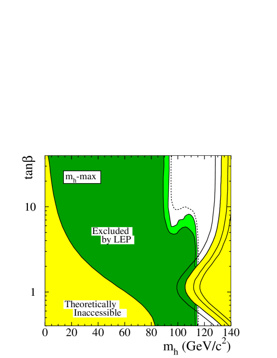
Figure 1.12: The LEP exclusion limit on the lightest CP even neutral Higgs boson.

1.3.4 The experimental status of the MSSM

Notwithstanding the theoretic soundness and the phenomenological advantages, discovery of supersymmetry has not yet been made, after decades of experimentations. No superpartners have yet been discovered at collider experiments. The general limits from direct experiments that could produce superpartners are not even very strong. They are also all model dependent, with varying significance. Limits from LEP on charged superpartners are near the kinematic limits except for models having near degeneracy of the charged sparticle and the LSP, in which case the decay products are very soft and hard to observe, giving weaker limits. So in most cases charginos and charged sleptons have limits of about 94 GeV. Gluinos and squarks have typical limits of about 308 GeV and 379 GeV respectively, except that if one or two squarks are lighter the limits on them are much weaker. For stops and sbottoms the limits are about 85 GeV.

There are no clear limits on neutralinos at the LEP. This is so because one can easily construct models where production of LSP’s are unobservable at the LEP. There are no general relations between neutralino masses and chargino or gluino masses, so limits on the latter do not imply limits on neutralinos. In typical models the limits are $M_{LSP}\gtrsim 46$ GeV, $M_{\widetilde{N}_{2}}\gtrsim 62.4$ GeV. Superpartners get mass from both the Higgs mechanism and from supersymmetry breaking, so one would expect them to typically be heavier than SM particles.

The direct searches have also put constraints on the Higgs mass. The combined constraint on the lightest CP even neutral Higgs field is shown in Figure 1.12.

Theoretically if MSSM explains electroweak symmetry breaking then one needs to reproduce Z mass in terms of soft-breaking masses, given by the relation,

$$m_{Z}^{2}=\frac{|m^{2}_{H_{d}}-m^{2}_{H_{u}}|}{\sqrt{1-\sin^{2}(2\beta)}}-m^{2}_{H_{u}}-m^{2}_{H_{d}}-2|\mu|^{2},$$ (1.96)

so if the soft-breaking masses are too large, it would lead to large finetuning. The parameters that are most sensitive to this issue are $M_{3}$ (basically the gluino mass) and $\mu$ which strongly affects the chargino and neutralino masses. Qualitatively one therefore expects rather light gluino, chargino, and neutralino masses. Argument in this direction leads to the following upper mass limits: $M_{\tilde{g}}\lesssim 500$ GeV; $M_{\widetilde{N}_{2}},$ $M_{\widetilde{C}}\lesssim 250$ GeV; and $M_{\widetilde{N}_{1}}\lesssim 100$ GeV. These are upper limits, seldom saturated in models. There are no associated limits on sfermions.

It is however expected that the LHC will finally sit on judgment for the existence of the MSSM [62]. At the LHC, production of gluinos and squarks by gluon-gluon and gluon-quark fusion usually dominate, unless the gluinos and squarks are heavier than 1 TeV or so. One can also have associated production of a chargino or neutralino together with a squark or gluino. Slepton pair production might be observable at the LHC [63] . Cross-sections for sparticle production at hadron colliders can be found in Refs. [64].

The decays of the produced sparticles result in final states with two neutralino LSPs, which escape the detector. The LSPs carry away at least $2m_{\tilde{N}_{1}}$ of missing energy, but at hadron colliders only the component of the missing energy that is manifest in momenta transverse to the colliding beams (denoted by $\not{E}_{T}$) is observable. So, in general the observable signals for supersymmetry at hadron colliders are $n$ leptons + $m$ jets + $\not{E}_{T}$. There are important Standard Model backgrounds to many of these signals, especially from processes involving production of $W$ and $Z$ bosons that decay to neutrinos, which provide the $\not{E}_{T}$. One must choose the $\not{E}_{T}$ cut high enough to reduce backgrounds from detector mismeasurements of jet energies. The jets$+\not{E}_{T}$ signature is one of the main signals currently being searched at LHC.

1.4 Conclusion and Outlook

The Standard Model (SM) of elementary particle physics provides a correct description of virtually all known microphysical nongravitational phenomena. However, there are a number of theoretical and phenomenological issues that the SM fails to address adequately: the gauge hierarchy problem, triggering electroweak symmetry breaking, gauge coupling unification, explanation of family structure and fermion masses, cosmological challenges including the issue of dark matter etc.

All these indicate the existence of new physics at around the 1 TeV mark, which can be probed by collider experiments and astrophysical observations. Low energy supersymmetry (SUSY) and compactified extra dimensions (EDs) provide theoretically sound and phenomenologically exciting frameworks to extend the SM and strengthen its foundations.

Supersymmetry, which is included in the most general set of symmetries of local relativistic field theories, has the virtue of solving the gauge hierarchy problem and is a popular choice of physics beyond the standard model. In the simplest supersymmetric world ($N=1$), each particle has a superpartner which differs in spin by $1/2$, and is related to the original particle by SUSY transformations, as discussed above. Since SUSY relates the scalar and fermionic sectors, the chiral symmetries which protect the masses of the fermions, also protect the masses of the scalars from quadratic divergences, leading to an elegant resolution of the hierarchy problem. We saw that apart from this, SUSY leads to unification of gauge couplings, triggers electroweak symmetry breaking radiatively, provides cold dark matter candidate and provides a framework to turn on gravity.

On the other hand, theories with extra dimensions have recently attracted enormous attention. The study of TeV scale extra dimensions that has taken place over the past few years has its origin in the ground breaking work of Arkani-Hamed, Dimopoulos and Dvali (ADD) [55]. Since that time, the extra dimensions have evolved from a single idea to a new paradigm of employing EDs as a tool to address a large number of outstanding issues that remain unanswerable in SM context. This in turn leads to phenomenological implications that can be tested at colliders and elsewhere. Various variants of EDs have been used in addressing various issues including hierarchy problem, electroweak symmetry breaking without Higgs boson, the generation of ordinary fermion and neutrino mass hierarchy, the CKM matrix, new sources of CP violation, grand unification while suppressing proton decay, new dark matter candidates, new cosmological perspectives, black hole productions at future colliders as a window on quantum gravity, novel mechanisms of SUSY breaking etc. Technical details of extra-dimensional theories will be given in Chapter 2.

For some time now, it is believed that string theory is a realistic attempt to provide an unified quantum picture of all known interactions in physics. Consistent string theories indicate the existence of supersymmetry and compactified extra dimensions in their low energy phenomenology. Though a rigorous connection between string theory and low energy phenomenological models with extra dimensions has not yet been possible, it provides enough motivation to study higher dimensional supersymmetric theories. From a purely phenomenological point of view, such higher dimensional supersymmetric theories have various virtues to their credit, including the explanation of fermion mass hierarchy from a different angle, providing a cosmologically viable dark matter candidate, interpretation of the Higgs as a quark composite leading to a successful electroweak symmetry breaking without the necessity of a fundamental Yukawa interaction, and lowering the unification scale down to a few TeV. Supersymmetrization provides a natural mechanism to stabilize the Higgs mass in extra dimensional scenarios. It is also worthwhile to note that all supersymmetric models in four dimensions necessarily introduce the paradigm of further new physics that controls SUSY breaking in this class of models. Embedding supersymmetric models in extra dimension provides various avenues to realize soft breaking of supersymmetry. The rest of this thesis will focus on the phenomenology of extra dimensions and their interface with supersymmetry.

Chapter 2 Probing Warped Extra dimension at the LHC

2.1 Extra dimensions

It is generally believed that some form of New Physics (NP) must exist beyond the Standard Model (SM) to explain its deficiencies. Though there are many candidates for NP, as discussed in Section 1.2, it will be up to experiments at future colliders, the Large Hadron Collider (LHC) and the proposed International Linear Collider (ILC), to reveal its true nature.

One possibility is that extra spatial dimensions will begin to show themselves at or near the TeV scale. The discovery of extra dimensions (ED) would produce a fundamental change in how we view the universe. The study of the physics of TeV-scale EDs that has taken place over the past few years has its origins in the ground breaking work of Arkani-Hamed, Dimopoulos and Dvali (ADD) [55]. Since that time EDs has evolved from a single idea to a new paradigm with various applications. Extra dimensions have been used as a tool to address the large number of outstanding issues that remain unanswerable in the SM context. This in turn has lead to other phenomenological implications which should be testable at colliders and elsewhere. A tentative list of some of these applications includes,

1. Addressing the hierarchy problem [55, 56].

2. Triggering electroweak symmetry breaking without a Higgs boson [65].

3. The generation of the ordinary fermion and neutrino mass hierarchy, the CKM matrix and new sources of CP violation [66].

4. TeV scale grand unification or unification without SUSY while suppressing proton decay [67].

5. New Dark Matter candidates and a new cosmological perspective [68, 69].

6. Black hole production at future colliders as a window on quantum gravity [70].

An amplified discussion of all these issues is beyond the scope of the present thesis. However it is clear from this list that EDs have found their way into essentially every area of interest in high energy physics providing strong motivation for exploring the phenomenology of ED in present and future colliders.

The spatial Vs temporal EDs: Consider a massless particle moving in 5d ‘Cartesian’ co-ordinates and assume that 5d Lorentz invariance holds. Then the square of the 5d momentum for this particle is given by $p^{2}=0=g_{MN}p^{M}p^{N}=-p_{0}^{2}+$p${}^{2}\pm p_{5}^{2}$ where $g_{MN}=diag(-1,1,1,1,\pm 1)$ is the 5d metric tensor. As usual $p_{0}$ is the particle energy, p² is the square of the particle 3-momentum and $p_{5}$ is its momentum along the 5th dimension. A positive sign before the fifth component of the metric represents a space like extra dimension whereas a negative fifth component corresponds to a time like extra dimension. The right hand side of the equality is zero because of the the assumption of zero mass in 5d. We can re-write the equation above in a more traditional form as $-p_{0}^{2}+$p${}^{2}=p_{\mu}p^{\mu}=\mp p_{5}^{2}$ and we recall, for particles which satisfy 4d Lorentz invariance, that $p_{\mu}p^{\mu}=-m^{2}$, which is just the square of the particle mass (note $\mu$ runs from 0 to 3 where as $M,N$ runs from 0 to 4). Notice, that if we choose a time-like extra dimension, the sign of the square of the mass of the particle will appear to be negative, i.e., the particle is a tachyon. Tachyons are well known to cause severe causality problems [71] something that is best avoided in any theory. This implies that we should pick the space-like solution. Thus to avoid tachyons appearing in our ED theories we must always choose EDs to be space-like and therefore we assume there will always be only one time like dimension [72].

The brane world scenario: ED models are typically structured to have a extra spatial dimension that is compactified with a suitable orbifolding symmetry. The compactification enables this spatial dimension to evade all observation of its existence at low energy. Only when the probing energy is of the order of the compactification length scale, does one begins to see the manifestation of the extra dimension. The end points of the compactified extra dimension are the location of four dimensional hyper-surfaces called the 3-branes. The observed four dimensional structure of the hithertho discovered space-time geometry corresponds to one of these 3-branes, see [75] for further details.

In this chapter we review the Warped extra dimension in Section 2.2, detailing the derivation of the anti-de Sitter metric that originates naturally from the Einsteins equations with negative cosmological constant, a review of the particle spectrum and their interaction is then made in the context of a warped extra dimension compactified on an orbifold with $S_{1}/\mathbb{Z}_{2}$ symmetry. In Section  2.3 we demonstrate that the loop contribution of the KK towers of quarks and gauge bosons emerging from the compactification would have a sizable numerical impact on the rates of $gg\to h$ and $h\to\gamma\gamma$, which are of paramount importance in the context of Higgs search at the LHC. This happens because the Higgs coupling to a pair of KK fermion-antifermion is not suppressed by the zero mode fermion mass and can easily be order one . The underlying reason is simple. Although the zero mode wave-functions of different flavors have varying overlap at the TeV brane depending on the zero mode masses, the KK profiles of all fermions have a significant presence at the TeV brane where the Higgs resides. As a result, the KK Yukawa couplings of different flavors are not only all large, they are also roughly universal, see Section 2.2.5. This large universal Yukawa coupling in the RS scenario constitutes the corner-stone of our study. On the contrary, in flat Universal Extra Dimension (UED) only the KK top Yukawa coupling is large, others being suppressed by the respective zero mode fermion masses. We provide comparative plots to demonstrate how the warping in RS fares against the flatness of UED for the processes under consideration.

2.2 Warped Extra Dimension

Taking in account the back-reaction of gravity to the presence of the branes themselves naturally leads to warped extra dimensions. Careful consideration of the back-reaction may be important, since if one has a 4d theory with only 4d sources, it will necessarily lead to an expanding universe with positive cosmological constant. On the other hand, if one has 4d sources in 5d geometry, one can balance the effects of the 4d brane sources by a 5d bulk cosmological constant thus reducing the effective 4d cosmological constant to zero, that is the 4d universe would still appear to be static and flat for an observer on a brane [74]. Now the 5d background itself is curved, which is clear from the fact that one had to introduce a bulk cosmological constant. In a sense there is a transfer of the curvature from the 4d branes, which are made flat, to the bulk which is now significantly curved [75]. This scenario was originally proposed by Rubakov and Shaposhnikov [74].

2.2.1 The Randall-Sundrum background

With this motivation, consider a 5d scenario with a non-vanishing 5d cosmological constant $\Lambda$ in the bulk. We are interested in solutions where the brane itself remains static and flat, preserving the 4d Lorentz invariance, while the extra dimension is curved. This implies that the induced metric at every point along the fifth dimension has to be the ordinary flat 4d Minkowski metric, and the components of the 5d metric depend only on the fifth coordinate $y$. The ansatz for the most general metric satisfying these properties is given by:

$$ds^{2}=e^{-A(y)}dx^{\mu}dx^{\nu}\eta_{\mu\nu}+dy^{2}.$$ (2.1)

The amount of curvature along the fifth dimension depends on the function $e^{-A(y)}$, which is therefore called the warp-factor. To go into the conformally flat frame, we need to make a coordinate transformation of the form $z=z(y)$. The coordinate transformation should not depend on the 4d coordinates $x$, which might induce off-diagonal terms in the metric. One can ensure that the metric be conformally flat in the new frame, if $dy$ and $dz$ are related by

$$e^{-A(z)/2}dz=dy,$$ (2.2)

such that the full metric in terms of the the $z$ coordinate will be:

$$ds^{2}=e^{-A(z)}(dx^{\mu}dx^{\nu}\eta_{\mu\nu}+dz^{2}).$$ (2.3)

Deriving the RS solution now reduces to the task of finding the function $A(z)$. To do this we first note that the above mentioned conformally flat metric leads to the following non-vanishing components of the Einstein tensor:

$$G_{55} = -\frac{3}{2}A^{\prime 2},$$

$$G_{\mu\nu} = -\frac{3}{2}\eta_{\mu\nu}(-A^{\prime\prime}+\frac{1}{2}A^{\prime 2}),$$ (2.4)

where $G_{MN}=R_{MN}-\frac{1}{2}g_{MN}R$.

This should agree with the solution of the 5d Einstein-Hilbert action,

$$S=-\int d^{5}x\sqrt{g}(M_{*}^{3}R+\Lambda).$$ (2.5)

One can then use the definition of the stress-energy tensor to find the Einstein equation:

$$G_{MN}=\kappa^{2}T_{MN}=\frac{1}{2M_{*}^{3}}\Lambda g_{MN}.$$ (2.6)

Comparing the $55$ component of the Einstein equation will then give:

$$\frac{3}{2}A^{\prime 2}=-\frac{1}{2M_{*}^{3}}\Lambda e^{-A}.$$ (2.7)

The first thing that we note is that a solution can only exist if the bulk cosmological constant is negative $\Lambda<0$. This means that the important case for us will be considering anti-de Sitter spaces, that is spaces with a negative cosmological constant. With a negative value of $\Lambda$ one can now solve for the function $A(z)$. It is given by,

$$e^{-A(z)}=\frac{1}{(kz+{\rm const.})^{2}},$$ (2.8)

where we have introduced

$$k^{2}=-\frac{\Lambda}{12M_{*}^{3}}.$$ (2.9)

To fix the constant in Eq. 2.8 we choose $e^{-A(0)}=1$, giving us,

$$e^{-A(z)}=\frac{1}{(kz+1)^{2}}.$$ (2.10)

The metric in the original $y$ coordinates can now be read off by recalling the relation between $z$ and $y$ given by

$$e^{-A(z)/2}dz=\frac{dz}{kz+1}=dy,$$ (2.11)

we get that (by choosing $y=0$ to correspond to $z=0$):

$$e^{-A(z)}=\frac{1}{(kz+1)^{2}}=e^{-2ky},$$ (2.12)

and so the RS metric in its more well-known form is finally given by:

$$ds^{2}=e^{-2ky}dx^{\mu}dx^{\nu}\eta_{\mu\nu}+dy^{2}.$$ (2.13)

However one still needs to check whether the 4d components $(G_{\mu\nu})$ of Eq. 2.2.1 and Eq. 2.6 are in agreement. In order to fulfill this condition we will find that the two branes at the two ends of the compactified extra dimension need to have equal and opposite brane tension which is related to the bulk cosmological constant. If we consider $V_{0}$ and $V_{1}$ are the tensions at two opposite branes, then we will find that they are related as follows,

$$\Lambda=-\frac{V_{0}^{2}}{12M_{*}^{3}},\ \ V_{1}=-V_{0}.$$ (2.14)

Thus there is a static flat solution only, if the above two fine tuning conditions are satisfied. For details see for example [75].

2.2.2 Compactification and KK Decomposition of Bulk Fields

Figure 2.1: A slice of AdS₅: The Randall-Sundrum scenario.

We are considering a scenario [56, 77] based on a non-factorizable geometry with an extra dimension as shown in Figure 2.1. In this scenario the fifth dimension $y$ is compactified on a $S^{1}/\mathbb{Z}_{2}$ orbifold of radius $R$, with $-\pi R\leq y\leq\pi R$. The orbifolding is needed to obtain chiral fermions in the zero mode of the KK tower, in agreement with the chiral fermions of the SM. The orbifold fixed points at $y=(0,\pi R)$ are also location of two 3-branes. The space-time between the two branes is simply a slice of $AdS_{5}$ geometry. The five dimensional metric is given by [56],

$$ds^{2}=e^{-2\sigma}\eta_{\mu\nu}dx^{\mu}dx^{\nu}+dy^{2}\,$$ (2.15)

where

$$\sigma=k|y|~{},$$ (2.16)

and $1/k$ is the AdS curvature radius and $\eta_{\mu\nu}={\rm diag}(-1,1,1,1)$. The natural mass scale associated with the brane at $y=0$ is the Plank scale ($M_{pl}$) and the corresponding 3-brane is called the Planck brane. The effective mass scale associated with the $y=\pi R$ brane is $M_{P}e^{-\pi kR}$, which is of the TeV order for $kR\simeq 12$. The corresponding 3-brane at $y=\pi R$ is called the Weak or TeV brane. This immediately provides a framework to address the hierarchy problem associated with fundamental scalars. Consider the scalar field (for example the Higgs scalar) confined to the TeV/Weak brane. Its action would be given by

$$S^{Higgs}=\int d^{4}x\sqrt{g^{5}}[g_{\mu\nu}D^{\mu}hD^{\nu}h-V(h)],\ \ \ V(h)=\lambda[(h^{\dagger}h)-v^{2})^{2}].$$ (2.17)

If the size of the extra dimension is $\pi R$, then the induced metric at the TeV brane is given by

$$g_{\mu\nu}^{5}|_{y=\pi R}=e^{-2k\pi R}\eta_{\mu\nu}.$$ (2.18)

Plugging this in for the above action we get that the action for the Higgs is given by

$$S^{Higgs}=\int d^{4}xe^{-4k\pi R}[e^{2k\pi R}\eta_{\mu\nu}\partial^{\mu}h\partial^{\nu}h-\lambda(h^{\dagger}h-v^{2})^{2}].$$ (2.19)

We can see that due to the non-trivial value of the induced metric on the TeV brane the Higgs kinetic term will not be canonically normalized. To get the action for the canonically normalized field, one needs a field redefinition $\tilde{h}\rightarrow e^{-k\pi R}h$. In terms of this field the action is

$$S^{Higgs}=\int d^{4}x[\eta_{\mu\nu}\partial^{\mu}\tilde{h}\partial^{\nu}\tilde{h}-\lambda[(\tilde{h}^{\dagger}\tilde{h})-(e^{-k\pi R}v)^{2}]^{2}].$$ (2.20)

This is exactly the action for a normal Higgs scalar, but with the vev (which sets the scale of all mass parameters) “warped down” to $\tilde{v}_{Higgs}=e^{-k\pi R}v$ thus solving the gauge hierarchy problem.

Till now we have discussed the brane bound fields (e.g Higgs field as in the previous example). But a natural generalization of the scenario is the one where the fields are allowed to access the 5d bulk. This requires a systematic study of the bulk fields. First we note that even though the space-time is 5 dimensional, we are confined to a four dimensional hyper-surface called the TeV brane. Thus we need to derive the effective four dimensional version of the 5d action by integrating out the fifth spatial component. The general 5 dimensional action of bulk fermions, scalars and vector bosons, is given by,

$$S_{5}=-\int d^{4}x\int dy\sqrt{-g}\,\Bigg{[}\frac{1}{4g^{2}_{5}}F^{2}_{MN}+\left|\partial_{M}\phi\right|^{2}+i\bar{\Psi}\gamma^{M}D_{M}\Psi+m^{2}_{\phi}|\phi|^{2}+im_{\Psi}\bar{\Psi}\Psi\Bigg{]}\,,$$ (2.21)

where $g={\rm det}(g_{MN})$, $F_{MN}=\partial_{M}V_{N}-\partial_{N}V_{M}$ and $D_{M}=\partial_{M}+\Gamma_{M}$ where $\Gamma_{M}$ is the spin connection given by $\Gamma_{\mu}=\frac{1}{2}\gamma_{5}\gamma_{\mu}\frac{d\sigma}{dy}$, $\Gamma_{5}=0$ for the metric given in Eq. 2.15. The bulk masses consistent with the orbifolding conditions are given by,

$$m^{2}_{\phi} = ak^{2}+b\sigma^{\prime\prime}\,,$$

$$m_{\Psi} = c\sigma^{\prime}\,,$$ (2.22)

where $a,b$ and $c$ are arbitrary dimensionless parameters and $\sigma$ is defined in Eq. 2.16.

After integrating out the compactified extra dimension the 4d Lagrangian can be written in terms of the zero modes and their KK towers. The fermionic [78], scalar and vector [79] fields can in general be expanded in KK modes as follows,

$$\Phi(x^{\mu},y)={1\over\sqrt{2\pi R}}\sum_{n=0}^{\infty}\Phi^{(n)}(x^{\mu})f_{n}(y)\,,$$ (2.23)

with

$$f_{n}(y)=\frac{e^{s\sigma/2}}{N_{n}}\left[J_{\alpha}(\frac{m_{n}}{k}e^{\sigma})+b_{\alpha}(m_{n})\,Y_{\alpha}(\frac{m_{n}}{k}e^{\sigma})\right]\,,$$ (2.24)

for $\Phi=\{\phi,e^{-2\sigma}\Psi_{L,R}\,A_{\mu}\}$ where

$$b_{\alpha}=-\frac{(-r+\frac{s}{2})J_{\alpha}(\frac{m_{n}}{k})+\frac{m_{n}}{k}J^{\prime}_{\alpha}(\frac{m_{n}}{k})}{(-r+\frac{s}{2})Y_{\alpha}(\frac{m_{n}}{k})+\frac{m_{n}}{k}Y^{\prime}_{\alpha}(\frac{m_{n}}{k})}~{},$$ (2.25)

and

$$N_{n}\simeq\frac{1}{\sqrt{\pi^{2}R~{}m_{n}~{}e^{-\pi kR}}}~{},$$ (2.26)

with $s=(4,1,2)$, $r=(b,\mp c,0)$ and $\alpha=(\sqrt{4+a},c\pm\frac{1}{2},1)$ respectively. The Kaluza Klein masses are determined by imposing boundary conditions on the solution given in Eq. 2.24. For even (odd) fields the boundary conditions are $\left.\left(\frac{df_{n}}{dy}-r\sigma^{\prime}f_{n}\right)\right|_{0,\pi R}=0$ $\left(f_{n}\Big{|}_{0,\pi R}=0\right)$. Thus we find that the KK masses are given by the roots of the equation,

$$b_{\alpha}(m_{n})=b_{\alpha}(m_{n}e^{\pi kR}).$$ (2.27)

In the limit that $m_{n}\ll k$ ,$\alpha>0$ and $kR\gg 1$ the Kaluza-Klein mass solutions are

$$m_{n}\simeq\left(n+\frac{1}{2}(\alpha-1)\mp\frac{1}{4}\right)\pi k~{}e^{-\pi kR}~{}$$ (2.28)

for $n=1,2,\dots$

It is to be noted that the masses of both even and odd KK fermions are identical and are given approximately by,

$$m_{n}^{\psi}\simeq\left(n+\frac{1}{2}|(c-\frac{1}{2})|-\frac{1}{4}\right)\pi k~{}e^{-\pi kR}.$$ (2.29)

This not clear from Eq 2.28 which is only true for $\alpha>0$. This requires a very careful study of the fermionic sector of the theory. The 5 dimensional action for the fermions is given by,

$$S_{5}=-\int d^{4}x\int dy\sqrt{-g}\,\Bigg{[}i\bar{\Psi}\gamma^{M}D_{M}\Psi+im_{\Psi}\bar{\Psi}\Psi\Bigg{]}\,,$$ (2.30)

where,

$$m_{\Psi} = c\sigma^{\prime}\,,$$ (2.31)

After integrating out the compactified extra dimension, the 4d Lagrangian can be written in terms of the zero modes and their KK towers. The fermionic [78] fields can in general be expanded in KK modes as follows,

$$\widehat{\Psi}_{L,R}(x^{\mu},y)={1\over\sqrt{2\pi R}}\sum_{n=0}^{\infty}\widehat{\Psi}_{L,R}^{(n)}(x^{\mu})f_{n}(y)\,,$$ (2.32)

The (L,R) correspond to the $\mathbb{Z}_{2}$ even and $\mathbb{Z}_{2}$ odd fermions respectively and $\widehat{\Psi}=e^{-2\sigma}\Psi_{L,R}$.

Where we have,

$$f_{n}(y)=\frac{e^{s\sigma/2}}{N_{n}}\left[J_{\alpha}(\frac{m_{n}}{k}e^{\sigma})+b_{\alpha}(m_{n})\,Y_{\alpha}(\frac{m_{n}}{k}e^{\sigma})\right]\,,$$ (2.33)

with

$$N_{n}\simeq\frac{1}{\sqrt{\pi^{2}R~{}m_{n}~{}e^{-\pi kR}}}~{},$$ (2.34)

and $s=(1)$, $r=(\mp c)$ and $\alpha=(c\pm\frac{1}{2})$.

The Kaluza Klein masses are determined by imposing boundary conditions on the solution given in Eq. 2.33. For even (odd) fields the boundary conditions are $\left.\left(\frac{df_{n}}{dy}-r\sigma^{\prime}f_{n}\right)\right|_{0,\pi R}=0$ $\left(f_{n}\Big{|}_{0,\pi R}=0\right)$.

For the even fields imposing the boundary condition gives rise to the two equations

$$b_{\alpha} = -\frac{(-r+\frac{s}{2})J_{\alpha}(\frac{m_{n}}{k})+\frac{m_{n}}{k}J^{\prime}_{\alpha}(\frac{m_{n}}{k})}{(-r+\frac{s}{2})Y_{\alpha}(\frac{m_{n}}{k})+\frac{m_{n}}{k}Y^{\prime}_{\alpha}(\frac{m_{n}}{k})}~{},$$ (2.35)

$$b_{\alpha}(m_{n}) = b_{\alpha}(m_{n}e^{\pi kR})\,.$$ (2.36)

These two conditions determine the values of $b_{\alpha}$ and $m_{n}$. Using the values of $r,s,$ and $\alpha$ and the recursion relations for the Bessel functions we get that,

$$b_{\alpha}(m_{n})=\frac{J_{\alpha-1}(\frac{m_{n}}{k})}{Y_{\alpha-1}(\frac{m_{n}}{k})}$$ (2.37)

The KK masses are approximately given by the roots of $J_{\alpha-1}(\frac{m_{n}}{k})=0$, but the roots of $J_{a}$ and $J_{-a}$ are identical so we can as well call it the root of $J_{|a|}$. In the limit that $m_{n}\ll k$ and $kR\gg 1$ the Kaluza-Klein mass solutions for $n=1,2,\dots$ are given by

$$m_{n}\simeq\left(n+\frac{1}{2}|\alpha-1|-\frac{1}{4}\right)\pi k~{}e^{-\pi kR}$$ (2.38)

$$m_{n}\simeq\left(n+\frac{1}{2}|(c-\frac{1}{2})|-\frac{1}{4}\right)\pi k~{}e^{-\pi kR}$$ (2.39)

since for even fields $\alpha=c+\frac{1}{2}$ thus $\alpha-1=c-\frac{1}{2}$

For the odd fields the continuity of $f_{n}$ at the boundaries implies that

$$f_{n}\Big{|}_{0,\pi R}=0\,,$$ (2.40)

and consequently

$$b_{\alpha}(m_{n}) = -\frac{J_{\alpha}(\frac{m_{n}}{k})}{Y_{\alpha}(\frac{m_{n}}{k})}\,,$$ (2.41)

$$b_{\alpha}(m_{n}) = b_{\alpha}(m_{n}e^{\pi kR})\,.$$ (2.42)

In this case one can check that the derivative of $f_{n}$ is continuous on the boundaries and does not lead to further conditions. As in the even case, an approximate solution for the Kaluza-Klein tower in the limit that $m_{n}\ll k$ and $kR\gg 1$ is

$$m_{n}\simeq\left(n+\frac{1}{2}|(c-\frac{1}{2})|-\frac{1}{4}\right)\pi k~{}e^{-\pi kR},$$ (2.43)

Thus the even and odd fields have degenerate KK mass which reaches minimum at $c=\frac{1}{2}$ when it has mass equal to the gauge boson. This is the value of c for which the fermion is in the conformal limit i.e when the bulk proffile of the fermions becone independent of the fifth dimension.

2.2.3 The zero mode profile

One of the major features of warped extra dimension is that, unlike the flat case the zero modes still have $y$ dependence which is generally exponential. The non-trivial zero mode bulk profiles lead to a possible explanation of the fermion mass hierarchy. Here we briefly summerize the general features of the zero mode fields in Table 2.1.

Field	Profile
scalar $\phi^{(0)}(y)$	$e^{(1\pm\sqrt{4+a})k|y|}$
fermion $\psi^{(0)}_{+}(y)$	$e^{\left(\frac{1}{2}-c\right)k|y|}$
vector $A_{\mu}^{(0)}(y)$	1
graviton $h_{\mu\nu}^{(0)}(y)$	$e^{-k|y|}$

Table 2.1: The zero mode profiles of bulk fields.

The equation of motion for the zero mode fields can be easily derived from Eq. 2.21 and is given by

$$(\pm t\partial_{t}-\nu)f_{0}(t)=0$$ (2.44)

where, $t=e^{\pi kR}e^{k|y|}$ and $\nu=\frac{m_{\Phi}}{k}$. The $m_{\Phi}$’s are given in Eq. 2.2.2. The solution of this equation with correct normalization is given by,

$$f_{o}^{(L,R)}(t)=\sqrt{\frac{1+2\nu}{1-\epsilon^{1+2\nu}}}\epsilon^{\pm\nu}e^{\pm\nu|k|y|}.$$ (2.45)

Only the left mode corresponding to the negative sign in the right hand side in Eq. 2.45, gives viable solution and the right mode does not exist as required by the orbifolding conditions.

To get the zero mode profile we need to look at the coefficient of the kinetic term. For example the kinetic term of the fermions is given by, $S_{kinetic}^{\psi}=-\int d^{4}x\int dy\sqrt{-g}\,[i\bar{\Psi}\gamma^{M}D_{M}\Psi]$ $\sim-\int d^{4}x\int dy\sqrt{-g}\,[i\bar{\Psi_{0}}\bar{f_{0}}\gamma^{M}D_{M}\Psi_{0}f_{0}]$ . Now note that $\sqrt{-g}=e^{-4k|y|}$ and $\gamma_{\mu}=E^{A}_{a}\gamma^{a}_{\mu}$ where $E^{A}_{a}=e^{|k|y}$. Further $\widehat{\Psi}=e^{-2\sigma}\Psi_{L,R}$. Putting everything together we get $S_{kinetic}^{\psi}=-\int d^{4}x\int dye^{(1-2c)k|y|}[i\bar{\Psi_{0}}\gamma^{a}_{M}D^{M}\Psi_{0}]$. Thus the zero mode profile is given by $e^{(\frac{1}{2}-c)k|y|}$.

The other zero mode profiles can be derived analogously. The gauge fields are kept in the conformal limit ($c=1/2$) i.e. they do not have any bulk profile and thus the zero mode is not localized at any point in the bulk. This is a direct consequence of the 5d gauge invariance. The gauge fields (any field in the conformal limit) couple to the two branes with equal strength whereas the other zero mode fields are localized near one point in the bulk having different couplings at the two branes.

2.2.4 Gauge Couplings

The generic gauge coupling part of the 5d action may be written as ,

$$S_{gauge}=\int d^{4}x\int dy\sqrt{-g}\,g_{5}\bar{\Psi_{i}}(x,y)\imath\gamma^{\mu}A_{\mu}(x,y)\Psi_{i}(x,y)~{}.$$ (2.46)

One can simply read off the coupling between all the zero mode fields, which can now be written as,

$$S_{gauge}^{(0)}=\int d^{4}x\int dy\sqrt{-g}\,g_{5}\left(\bar{\Psi_{i}}(x)^{(0)}f^{(0)}_{i}(y)\imath E^{a}_{A}\gamma^{\mu}_{a}A_{\mu}(x)^{(0)}f^{A}_{(0)}(y)\Psi_{i}(x)^{(0)}\right)\times\left(\frac{1}{\sqrt{2\pi R}}\right)^{3}$$ (2.47)

where $E^{a}_{A}=e^{k|y|}$ is the vierbein. The 4d gauge coupling for the fermion of flavor $i$ is given by,

$$g_{4,i}=\int dy\sqrt{-g}\,g_{5}E^{a}_{A}\left(\frac{1}{\sqrt{2\pi R}}\right)^{3}(f^{(0)}_{i}(y))^{2}f^{A}_{(0)}(y),$$ (2.48)

remembering that all the gauge bosons are put in the conformal limit (implies $f^{A}_{(0)}(y)=1$) we can explicitly perform the y integral to get,

$$g_{4,i}=\frac{g_{5}}{\sqrt{2\pi R}}.$$ (2.49)

This clearly shows that the zero mode couplings are independent of the flavor index, thus gauge invariance of the theory is not compromised by localizing the zero modes at different location in the bulk. Couplings of the zero mode fermions to the KK modes of the gauge bosons may lead to four-fermion interactions and FCNC processes that are highly constrained. Using the expression for the zero-mode fermion , the gauge coupling of a gauge boson Kaluza-Klein mode $n$ to the zero-mode fermions is

$$g^{(n)}=g\left(\frac{1-2c}{e^{(1-2c)\pi kR}-1}\right)\frac{k}{N_{n}}\int_{0}^{\pi R}dy\,e^{(1-2c)\sigma}\left[J_{1}(\frac{m_{n}}{k}e^{\sigma})+b_{1}(m_{n})Y_{1}(\frac{m_{n}}{k}e^{\sigma})\right]~{}.$$ (2.50)

\begin{picture}(0.0,0.0) \end{picture}

Figure 2.2: The ratio of the gauge couplings, $g^{(n)}/g$, for $n=1$ (dotted line), $n=2$ (solid line) and $n=3$ (dashed-dotted line), as a function of the dimensionless fermion mass parameter $c$ [77].

When $c$ takes a large negative value, the fermion is localized near the TeV-brane and the ratio $g^{(1)}/g$ approaches the asymptotic limit $g^{(1)}/g\simeq\sqrt{2\pi kR}\simeq 8.4$, which corresponds to a fermion localized near the TeV-brane. This leads to a restrictive lower bound on the first excited Kaluza-Klein mass scale. At the conformal limit $c=1/2$, the coupling vanishes due to the conservation of the 5-momentum at this limit. For $c>1/2$, the coupling quickly becomes universal for all fermion masses. Nevertheless, the FCNC and other constraints will dissappear if a KK parity is induced into the theory. In what follows we will see that various other considerations will also lead us to introduce a KK parity into the theory. Thus we will restrict the rest of this discussions to models where KK parity is a good symmetry of the theory.

2.2.5 Yukawa Structure

We note that the fermions and their superpartners have identical coupling to the Higgs. Thus in what follows, we only consider the Yukawa coupling of the fermion. The Higgs boson is localized on the TeV brane and thus the 5d Higgs field may be written as,

$$H(x,y)=H(x)\delta(y-\pi R)$$ (2.51)

Figure 2.3: The variation of the Yukawa couplings with $c_{i}$.

Using Eq. 2.51 and Eq. 2.23, we find that the 5d Yukawa term is given by,

$$S_{y}=\int d^{4}x\int dy\,\sqrt{-g}\,\,\lambda^{(5)}_{ij}H(x)\Big{(}\bar{\Psi}_{iL}(x,y)\Psi_{jR}(x,y)+h.c.\Big{)}\delta(y-\pi R)$$ (2.52)

where, $\Psi_{i,L/R}$ is a chiral fermion with flavor index $i$ and $H(x)$ is the Higgs boson . This can be written as,

$$S_{y} = \int d^{4}x\,\,\left[\lambda_{ij}H(x)\Big{(}\bar{\Psi}^{(0)}_{iL}(x)\Psi^{(0)}_{jR}(x)+h.c.+\dots\Big{)}\right.$$

$$+ \left.\sum\lambda_{ij}^{(n)}H(x)\Big{(}\bar{\Psi}^{(n)}_{iL}(x)\Psi^{(n)}_{jR}(x)+h.c.+\dots\Big{)}\right]$$

Considering a left-right symmetric model, we find that the zero mode Yukawa couplings ($\lambda_{ij}$) are given by,

$$\lambda_{ij}=\frac{(1/2-c_{i})\lambda_{ij}^{(5)}k}{e^{(1-2c_{i})\pi kR}-1}e^{(1-2c_{i})\pi kR},~{}$$ (2.54)

If we assume $\lambda_{ij}^{(5)}k\sim 1$ for all $i,j$ we can still generate hierarchal Yukawa structure by tuning the $c$ parameter. This is the explanation of the fermion hierarchy problem in warped extra dimension where the warping factor is used to generate the variation in the zero mode fermion masses. The Yukawa couplings of the KK modes can be read off by inserting Eq. 2.23 in Eq. 2.52 and comparing with Eq. 2.2.5 and are given by,

$${\lambda}_{i}^{n} = \sqrt{-g}{\lambda}_{ij}^{(5)}e^{-\pi kR}\frac{e^{4\pi kR}}{2\pi R}{\Big{(}f_{n}(\pi R)\Big{)}}^{2}$$ (2.55)

$$= \sqrt{-g}e^{3\pi kR}{\lambda}_{ij}^{(5)}\pi m_{n}{\left[J_{\alpha}\Big{(}\frac{m_{n}}{k}e^{\pi kR}\Big{)}+b_{\alpha}(m_{n})Y_{\alpha}\Big{(}\frac{m_{n}}{k}e^{\pi kR}\Big{)}\right]}^{2}$$

With the approximations $m_{n}\ll k$, $kR\gg 1$ and ${\lambda}_{ij}^{(5)}k=1$, we can expand the Bessel function in the asymptotic limit as,

$$J_{n}(x)=\sqrt{\frac{2}{\pi x}}\cos(x-(2|n|+1)\frac{\pi}{4}$$ (2.56)

Using this form we find that the KK Yukawa couplings are given by

$${\lambda}_{i}^{n}\sim{\cos}^{2}\Big{(}\left[n+\frac{|c-\frac{1}{2}|-|c+\frac{1}{2}|}{2}-\frac{1}{2}\right]\pi\Big{)}.$$ (2.57)

This clearly shows that all the even KK modes have Yukawa couplings equal to unity independent of their zero mode Yukawa couplings for $|c|>0.5$. The odd KK modes do not couple to the brane bound Higgs at all. The important observation is that the couplings are nearly independent of the $c_{i}$ parameter, the radius of compactification (R) and the KK number (n). The actual numerical values of the Yukawa couplings are plotted as a function of $c_{i}$ in Figure 2.3.

$f_{i}$	$e$	$\mu$	$\tau$	$u$	$d$	$c$	$s$	$t$	$b$
$c_{i}$	0.61	0.52	0.40	0.62	0.57	0.52	0.52	-0.50	0.26
$m^{(1)}_{i}$	1073	1013	1066	1080	1047	1013	1013	1667	1160
$\lambda_{n}$	1	1	.9	1	1	1	1	1	.5

Table 2.2: The $c_{i}$ parameters and $m^{(1)}_{i}$ (in GeV) for different flavors are shown for $kR=12.06$ and $\tan\beta={\langle H_{u}^{0}\rangle}/{\langle H_{d}^{0}\rangle}=10$. For this choice, the mass gap between the consecutive KK states is $m^{(n+1)}-m^{(n)}=1333$ GeV, irrespective of $c_{i}$. The corresponding $n=1$ KK mass for gauge boson is $1$ TeV.

2.2.6 Radius stabilization

The radius of the model so far has been treated as a given constant, and it was found that radius $R$ has to be $R\sim 12/k$ in order for the hierarchy problem to be resolved. This raises several important issues, that needs to be addressed: Since the radius is not dynamically fixed at the moment, but rather just set to its desirable value, there will be a corresponding massless scalar field in the effective theory, which corresponds to the fluctuations of the radius of the extra dimensions, called the radion [80, 81, 82, 83]. The masslessness of this field is related to the fact that the RS solution discussed until now did not make any reference to the size of the extra dimension. This means that in the effective theory this parameter is also arbitrary, and thus has no non-trivial potential. Thus it can have no mass. This massless radion would contribute to Newton’s law and result in violations of the equivalence principle (would cause a fifth force), which is phenomenologically unacceptable, and therefore the radius has to be stabilized (making the radions massive). Even then the radius has to be stabilized at a somewhat larger than natural value (we need $kR\sim 12$, while one would expect $R\sim 1/k$). This reintroduces the hierarchy/finetuning problem. We have seen that one needed two fine tunings to obtain the static RS solution, one of which was equivalent to the vanishing of the 4d cosmological constant.

A mechanism for radius stabilization should address the above mentioned issues. The solution for stabilization of the size of the extra dimension was proposed by Goldberger and Wise [80], and is known as the Goldberger-Wise (GW) mechanism. Radius stabilization at non-trivial values of the radius occurs dynamically, where different forces, some of which would like to drive the extra dimension very large, and some very small, are brought into play. Then there is a chance that these forces may balance each other at some value and a stable non-trivial minimum for the radius could be found. A possible way to find such a tension between large and small radii is if there is a tension between a kinetic and a potential term of a field, one which would want derivatives to be small (and thus large radii) and the other which would want small radii to minimize the potential. The Goldberger and Wise mechanism uses exactly this scenario. A bulk scalar field is introduced into the model, and a bulk mass term is added. This will result in a non-trivial potential for the radius, due to the bulk mass the radius would want to be as small as possible to minimise the potential. If there is also a non-trivial profile (a vev that is changing with the extra dimensional coordinate) for this scalar, then the kinetic term would want the radius to be as large as possible, so as to minimize the kinetic energy in the 5th direction. Then there would be a non-trivial minimum for the radius. The non-trivial profile for the scalar is generated by adding a brane potentials for this scalar on both fixed points, which have minima at different values from each other. The back-reaction of the metric to the presence of the scalar field in the bulk will be important. Simultaneous solution of the Einstein and the bulk scalar equations are required, to have the back-reaction exactly under control [85, 84, 86, 87]. Denote the scalar field in the bulk by $\Phi$, and consider the action

$$\int d^{5}x\sqrt{g}\left[-M_{*}^{3}R++\frac{1}{2}(\nabla\Phi)^{2}-V(\Phi)\right]-\int d^{4}x\sqrt{g_{4}}\lambda_{P}(\Phi)-\int d^{4}x\sqrt{g_{4}}\lambda_{T}(\Phi),$$ (2.58)

where the first term is the usual 5d Einstein-Hilbert action and the bulk action for the scalar field, while the next two terms are the brane induced potentials for the scalar field on the Planck and the TeV branes. We will denote the 5d Newton constant by $\kappa^{2}=1/2M_{*}^{3}$, and look for an ansatz of the background metric again of the generic form as in the RS case to maintain 4d Lorentz invariance:

$$ds^{2}=e^{-2A(y)}\eta_{\mu\nu}dx^{\mu}dx^{\nu}+dy^{2}.$$ (2.59)

The Einstein equations are given by:

$$4A^{\prime 2}-A^{\prime\prime}=-\frac{2\kappa^{2}}{3}V(\Phi_{0})-\frac{\kappa^{2}}{3}\sum_{i=P,T}\lambda_{i}(\Phi_{0})\delta(y-y_{i})$$

$$A^{\prime 2}=\frac{\kappa^{2}}{12}\Phi_{0}^{\prime 2}-\frac{\kappa^{2}}{6}V(\Phi_{0}).$$ (2.60)

And the bulk scalar equation of motion in the warped space, derived from the generic scalar equation is given by,

$$\partial_{\mu}\sqrt{g}g^{\mu\nu}\partial_{\nu}\Phi=\frac{\partial V}{\partial\Phi}\sqrt{g}.$$ (2.61)

By substituting the scalar and metric ansatz into this equation we get

$$\Phi_{0}^{\prime\prime}-4A^{\prime}\Phi_{0}^{\prime}=\frac{\partial V}{\partial\Phi_{0}}+\sum_{i}\frac{\partial\lambda_{i}(\Phi_{0})}{\partial\Phi}\delta(y-y_{i}).$$ (2.62)

We can separate these equations into the bulk equations that do not contain the delta functions, and the boundary conditions are obtained by matching the coefficients of the delta functions at the fixed points. The boundary conditions derived this way are sometimes also called the jump equations, which in our case will be given by

$$[A^{\prime}]_{i}=\frac{\kappa^{2}}{3}\lambda_{i}(\Phi_{0}),$$

$$[\Phi_{0}^{\prime}]_{i}=\frac{\partial\lambda_{i}(\Phi_{0})}{\partial\Phi}.$$ (2.63)

The bulk equations, Eq. 2.2.6-2.62, together with these boundary conditions form the equations of the coupled gravity-scalar system. These are coupled second order differential equations. Let us assume that the solution to the system of equations above are given by $A(y),\Phi_{0}(y)$. Where the superpotential function $W(\Phi)$ is defined via the equations

$$A^{\prime}\equiv\frac{\kappa^{2}}{6}W(\Phi_{0}),$$

$$\Phi_{0}^{\prime}\equiv\frac{1}{2}\frac{\partial W}{\partial\Phi}.$$ (2.64)

If we use these expressions for $A^{\prime}$ and $\Phi_{0}^{\prime}$ in the Einstein and scalar equations consistancy will demand the following relation:

$$V(\Phi)=\frac{1}{8}\left(\frac{\partial W}{\partial\Phi}\right)^{2}-\frac{\kappa^{2}}{6}W(\Phi)^{2},$$ (2.65)

and the corresponding jump conditions are,

$$\frac{1}{2}[W(\Phi_{0})]_{i}=\lambda_{i}(\Phi_{0}),$$

$$\frac{1}{2}[\frac{\partial W}{\partial\Phi}]_{i}=\frac{\partial\lambda_{i}(\Phi_{0})}{\partial\Phi}.$$ (2.66)

It is somewhat difficult to derive a superpotential for a specific potential. Generically the bulk potential should include a cosmological constant term (independent of $\Phi$) and a mass term (quadratic in $\Phi$), but for simplicity we neglect them. So we choose [85],

$$W(\Phi)=\frac{6k}{\kappa^{2}}-u\Phi^{2}.$$ (2.67)

The first term is just what one needs for a cosmological constant, while the second term will provide the mass term when taking the derivative. The jump conditions are satisfied if,

$$\lambda(\Phi)_{\pm}=\pm W(\Phi_{\pm})\pm W^{\prime}(\Phi_{\pm})(\Phi-\Phi_{\pm})+\gamma_{\pm}(\Phi-\Phi_{\pm})^{2},$$ (2.68)

where $\Phi_{\pm}$ are the values of the scalar field at the two branes, which we will also denote by $\Phi_{+}=\Phi_{P}$ at the Planck brane, and $\Phi_{-}=\Phi_{T}$ at the TeV brane. Then the solution is given by,

$$\Phi_{0}(y)=\Phi_{P}e^{-uy}.$$ (2.69)

From this, the value of the scalar field at the TeV brane is determined to be

$$\Phi_{T}=\Phi_{P}e^{-uR}.$$ (2.70)

This means that the radius is no longer arbitrary, but given by

$$R=\frac{1}{u}\ln\frac{\Phi_{P}}{\Phi_{T}}.$$ (2.71)

The value of the radius is determined by the equations of motion, which is exactly what we were after. This is the GW mechanism.

The metric background will then be obtained from the equation

$$A^{\prime}=\frac{\kappa^{2}}{6}W(\Phi_{0})=k-\frac{u\kappa^{2}}{6}\Phi_{P}^{2}e^{-2uy}$$ (2.72)

given by the solution

$$A(y)=ky+\frac{\kappa^{2}\Phi_{P}^{2}}{12}e^{-2uy}.$$ (2.73)

The first term is the usual RS warp factor (remember that $A$ has to be exponentiated to obtain the metric), while the second term is the back-reaction of the metric to the non-vanishing scalar field in the bulk. We will assume that the back-reaction is small, and thus that $\kappa^{2}\Phi_{P}^{2},\kappa^{2}\Phi_{T}^{2}\ll 1$, and that $v>0$. The values of $\Phi_{P}$ and $\Phi_{T}$ are determined by the bulk and brane potentials, so $\Phi_{P}/\Phi_{T}$ is a fixed value. Since we want to generate the right hierarchy between the Planck and weak scales we need to ensure that

$$kR\sim 12,$$ (2.74)

from which we get that

$$\frac{k}{u}\ln\left(\frac{\Phi_{P}}{\Phi_{T}}\right)\sim 12,$$ (2.75)

which implies that $u/k$ does not need to be exponentially small. This ratio sets the hierarchy in the RS model, and we can see that indeed one can generate this hierarchy using the GW stabilization mechanism by a very modest tuning of the input parameters of the theory.

Once the radius is stabilized using a non-trivial potential, we know that the radion is no longer massless. Next we find the radion mass [87, 89], see also [81, 82, 88]. For this, we need to find the scalar excitations of the coupled gravity-scalar system. This can be parameterized in the following way:

$$ds^{2}=e^{-2A-2F(x,y)}\eta_{\mu\nu}dx^{\mu}dx^{\nu}+(1+G(x,y))^{2}dy^{2},$$

$$\Phi(x,y)=\Phi_{0}(y)+\varphi(x,y).$$ (2.76)

At this moment it looks like there would be three different scalar fluctuations, $F,G$ and $\varphi$. However, if we plug this ansatz into the Einstein equation the 4d off-diagonal $\mu\nu$ components are satisfied only if

$$G=2F,$$ (2.77)

while the $\mu 5$ components imply the following further relation among the fluctuations:

$$\varphi=\frac{1}{\Phi_{0}^{\prime}}\frac{3}{\kappa^{2}}(F^{\prime}-2A^{\prime}F).$$ (2.78)

This means, that in the end there is just a single independent scalar fluctuation in the coupled equation, which we can choose to be $F$. Consistency of the Einstein equations lead to the following equation:

$$F^{\prime\prime}-2A^{\prime}F^{\prime}-4A^{\prime\prime}F-2\frac{\Phi_{0}^{\prime\prime}}{\Phi_{0}^{\prime}}F^{\prime}+4A^{\prime}\frac{\Phi_{0}^{\prime\prime}}{\Phi_{0}^{\prime}}F=e^{2A}\Box F$$ (2.79)

in the bulk and the following boundary condition:

$$(F^{\prime}-2A^{\prime}F)_{i}=0.$$ (2.80)

Let us first assume that there is no stabilization mechanism, that is the background is exactly the RS background given by $A=k|y|$, and $\Phi_{0}=0$. In this case most of the terms in the above equation disappear, and we are left with

$$F^{\prime}-2kF=e^{2ky}m^{2}F,\ \ (F^{\prime}-2kF)_{i}=0.$$ (2.81)

The only solution is for $m^{2}=0$, and the wave function of the un-stabilized radion will be given by

$$F(y)=e^{2k|y|}.$$ (2.82)

The metric corresponding to radion fluctuations in the unstabilized RS model corresponds to

$$ds^{2}=e^{-2k|y|-2e^{k|y|}f(x)}\eta_{\mu\nu}dx^{\mu}dx^{\nu}+(1+2e^{2k|y|}f(x))dy^{2}.$$ (2.83)

This is a single scalar mode, that is exponentially peaked at the TeV brane, just like all the graviton KK modes.

To find the radion mass for the case with GW stabilization, we simply need to plug into Eq. 2.79 the full background for $A$ and $\Phi_{0}$ with stabilization:

$$F^{\prime\prime}-2A^{\prime}F^{\prime}-4A^{\prime\prime}F+2uF^{\prime}-4uA^{\prime}F+m^{2}e^{2A}F=0.$$ (2.84)

To find the leading term for the radion mass we expand in terms of the back-reaction of the metric in the parameter $l=\kappa\Phi_{P}/\sqrt{2}$, and obtain the mass of the radion

$$m_{radion}^{2}=\frac{4l^{2}(2k+u)u^{2}}{3k}e^{-2(u+k)r}.$$ (2.85)

The radions coupling to the SM particles offers a rich phenomenology which is beyond the scope of this discussion.

2.3 Probing warped extra dimension via ${gg\to h}$ and ${h\to\gamma\gamma}$ at LHC

This section closely follow the work published in the paper: G. Bhattacharyya and T. S. Ray, “Probing warped extra dimension via gg $\rightarrow$ h and h $\rightarrow\gamma\gamma$ at LHC,” Phys. Lett.  B 675 (2009) 222 [arXiv:0902.1893 [hep-ph]].

For an intermediate mass ($<$ 150 GeV) Higgs boson, the relevance of its production at the CERN Large Hadron Collider (LHC) via gluon fusion ($gg\to h$) and its subsequent decay into two photons ($h\to\gamma\gamma$) cannot be over-emphasized. Since these are loop induced processes, a natural question arises as how sensitive these processes are to the existence of new physics. In this chapter, we explore such a possibility by embedding the Standard Model (SM) in a Randall-Sundrum (RS) warped geometry [56], where the bulk is a slice of Anti-de Sitter space (AdS₅) accessible to some or all SM particles [91, 77]. The virtues of such a scenario include a resolution of the gauge hierarchy problem caused by the warp factor [56], and an explanation of the hierarchy of fermion masses by their respective localizations in the bulk keeping the Higgs confined at the TeV brane [92]. Besides, the smallness of the neutrino masses could be explained [78], and light KK states would lead to interesting signals at LHC [93]. We demonstrate that the loop contribution of the KK towers of quarks and gauge bosons emerging from the compactification would have a sizable numerical impact on the $gg\to h$ and $h\to\gamma\gamma$ rates. This happens because the Higgs coupling to a pair of KK fermion-antifermion is not suppressed by the zero mode fermion mass and can easily be order one. The underlying reason is simple. Although the zero mode wave-functions of different flavors have varying overlap at the TeV brane depending on the zero mode masses, the KK profiles of all fermions have a significant presence at the TeV brane where the Higgs resides. As a result, the KK Yukawa couplings of different flavors are not only all large, they are also roughly universal. This large universal Yukawa coupling in the RS scenario constitutes the corner-stone of our study. On the contrary, in flat Universal Extra Dimension (UED) only the KK top Yukawa coupling is large, others being suppressed by the respective zero mode fermion masses. We provide comparative plots to demonstrate how the warping in RS fares against the flatness of UED for the processes under consideration.

2.3.1 Contribution of KK states to ${\sigma(gg\to h)}$

The process $gg\rightarrow h$ proceeds through fermion triangle loops. The SM expression of the cross section is given by ($\tau_{q}\equiv 4m_{q}^{2}/m_{H}^{2}$)

$$\sigma_{gg\rightarrow h}^{\rm SM} = \frac{\alpha_{s}^{2}}{576\pi v^{2}}\left|\sum_{q}A_{q}(\tau_{q})\right|^{2}\,\,,~{}~{}{\rm where}~{}~{}\left.A_{q}(\tau_{q})\right|_{\rm SM}=2\tau_{q}[1+(1-\tau_{q})f(\tau_{q})]~{},$$ (2.86)

with $f(\tau)={\rm arcsin}^{2}\left(\frac{1}{\sqrt{\tau}}\right)~{}{\rm for}~{}\tau\geq 1,$ and $f(\tau)=-\frac{1}{4}\left[{\rm ln}\left(\frac{1+\sqrt{1-\tau}}{1-\sqrt{1-\tau}}\right)-i\pi\right]^{2}{\rm for}~{}\tau<1~{}$. Above, $\alpha_{s}$ is the QCD coupling at the Higgs mass scale, $v$ is the Higgs vacuum expectation value and $A_{q}$ is the loop amplitude from the $q$th quark. In the SM, the dominant contribution comes from the top quark loop. Now, there will be additional contributions from the KK quarks. Importantly, due to the large universal KK Yukawa couplings, not only the KK top but also the KK modes of other quarks would have sizable contribution. Indeed, the lightest modes ($n=1$) would have dominant contributions. Setting the KK Yukawa couplings to unity, as suggested by Eq. 2.57, we derive the amplitude of the $n$th KK mediation of the $q$th flavor, with the same normalization of Eq. 2.86, as

$$\left.A_{q}(\tau_{q_{n}})\right|_{\rm KK}=\frac{4v^{2}}{m_{h}^{2}}\left[1+(1-\tau_{q_{n}})f(\tau_{q_{n}})\right].$$ (2.87)

In 5d the sum over $n$ yields a finite result. Eq. 2.87 is different from the UED result [94] in two ways: (i) we have set the KK Yukawa coupling to unity irrespective of quark flavors, while in UED the KK Yukawa coupling is controlled by zero mode masses; (ii) in UED there is an additional factor of 2 because both $\mathbb{Z}_{2}$ even and odd KK modes contribute, while in RS the odd modes do not couple to the brane-localized Higgs. In Figure 2.5, we have plotted the variation with $m_{h}$ of the deviation of the production cross section $\sigma_{\rm RS}(gg\to h)$ from its SM expectation $\sigma_{\rm SM}(gg\to h)$ normalized by the SM value. The dominant QCD correction cancels in this normalization. We have chosen four reference values of $m_{\rm KK}$ ($=1.0,1.5,2.0$ and $3.0$ TeV), where $m_{\rm KK}$ is the KK mass of the $n=1$ gauge bosons, which also happens to be the lightest KK mass in the bulk (corresponding to the conformal limit, $c=1/2$ for fermions). For $m_{h}$ below 150 GeV, the deviation is quite substantial (close to 45%) for $m_{\rm KK}=1$ TeV. For larger $m_{\rm KK}=$ 1.5 (3.0) TeV, the effect is still recognizable, around 18% (5%). In the inset, we exhibit a comparison between RS and UED contributions to the same observable, where the KK mass scales of the two scenarios, namely $m_{\rm KK}$ for RS and $1/R$ for UED, have been assumed to be identical ($=1$ TeV). For $m_{h}<$ 150 GeV, the RS contribution is about 2.5 times larger than the UED contribution, while the margin slightly goes down with increasing $m_{h}$. This factor 2.5 can be understood in the following way: In RS, five $n=1$ KK flavors (except the KK top) have mass around $m_{\rm KK}$ with order one Yukawa coupling. So naively we would expect a factor of 5 enhancement relative to UED. But in UED both $\mathbb{Z}_{2}$ even and odd modes contribute. This reduces the overall enhancement factor in RS over UED to about 2.5.

2.3.2 Contribution of KK states to ${\Gamma(h\to\gamma\gamma)}$

The $h\to\gamma\gamma$ process proceeds through fermion triangles as well as via gauge loops along with the associated ghosts. The decay width in the SM can be written as

$$\Gamma_{h\rightarrow\gamma\gamma}=\frac{\alpha m_{h}^{3}}{256\pi^{3}v^{2}}\left|\sum_{f}N_{c}^{f}Q_{f}^{2}A_{f}(\tau_{f})+A_{W}(\tau_{W})\right|^{2}\,,$$ (2.88)

where $\alpha$ is the electromagnetic coupling at the Higgs mass scale. The expression for $A_{f}$ is given in Eq. 2.86, and the dominant SM contribution to $A_{f}$ comes from the top quark loop. The $W$-loop amplitude in the SM is given by

$$\left.A_{W}(\tau_{W})\right|_{\rm SM}=-\left[2+3\tau_{W}+3\tau_{W}(2-\tau_{W})f(\tau_{W})\right]\,.$$ (2.89)

We derive the KK contribution of the gauge sector as

$$\left.A_{W}(\tau_{W_{n}})\right|_{\rm KK}=-\left[2+3\tau_{W}+3\tau_{W}(2-\tau_{W_{n}})f(\tau_{W_{n}})-2(\tau_{W_{n}}-\tau_{W})f(\tau_{W_{n}})\right].$$ (2.90)

Again, the sum over $n$ yields finite result and in the limit of large KK mass the KK contribution decouples. Our Eq. 2.90 is very different from the corresponding UED expression [94], primarily because the Higgs is confined at the brane in the present scenario while it resides in the bulk in UED. In Figure 2.5, we have plotted the decay width $\Gamma(h\to\gamma\gamma)$ in RS relative (and normalized as well) to the SM. Again, the four choices of $m_{\rm KK}$ are 1.0, 1.5, 2.0 and 3.0 TeV. There is a partial cancellation between quark and gauge boson loops, both in real and imaginary parts, not only for the zero mode but also for each KK mode. The meeting of the four curves just above the $m_{h}=2m_{t}$ threshold is a consequence of the above cancellation and at the meeting point the SM contribution overwhelms the KK contribution. Unlike in Figure 2.4, we witness both suppression and enhancement with respect to the SM contribution. The inset carries an illustration how RS fares against UED for identical KK masses.

Figure 2.4: The fractional deviation (from the SM) of the $gg\rightarrow h$ production cross section in RS is plotted against the Higgs mass. The four curves correspond to four different choices of $m_{\rm KK}$. In the inset, we have compared the UED contribution for $1/R=1$ TeV with the RS contribution for $m_{\rm KK}=1$ TeV.

Figure 2.5: Same as in Figure 2.5, except that the fractional deviation in $h\to\gamma\gamma$ decay width is plotted.

Next we construct a variable $R=\sigma_{gg\to h}~{}\Gamma_{h\to\gamma\gamma}$. In Figure 2.6, we have studied variation of $(R_{\rm RS}-R_{\rm SM})/R_{\rm SM}$ with $m_{h}$. For $m_{\rm KK}=$ 1.0, 1.5, 2.0 and 3.0 TeV, the fractional changes in $R$ are 30%, 14%, 8% and 4%, respectively, for $m_{h}<150$ GeV. The comparison shown in the inset shows that RS wins over UED roughly by a factor of 2 for identical KK scale for $m_{h}<150$ GeV. Incidentally, our UED plots in the insets of all the three figures are in complete agreement with [94]. See also [95] for a numerical simulation of the Higgs signal at LHC in the UED context.

2.4 Conclusions

In conclusion, we highlight the core issues: In the RS scenario, the brane-bound Higgs can have order one Yukawa coupling with the KK fermions of all flavors. Such large KK Yukawa couplings can sizably enhance the Higgs production via gluon fusion and alter the Higgs decay width into two photons, provided the KK masses are in a regime accessible to the LHC. Because of the proactive involvement of more flavors inside the loop, the effect in RS is significantly stronger (typically, by a factor of 2 to 2.5) than in UED for similar KK masses. Admittedly, this advantage in RS is somewhat offset by the fact that the lightest KK mass in UED can be as low as 500 GeV thanks to the KK-parity, while in RS a KK mass below 1.5 TeV would be difficult to accommodate (see below). However, attempts have been made to impose KK parity in warped cases as well [90].

Electroweak precision tests put a severe lower bound on $m_{\rm KK}$ ($\sim 10$ TeV) [96]. To suppress excessive contribution to $T$ and $S$ parameters, the gauge symmetry in the bulk is extended to ${\rm SU(2)_{L}\times SU(2)_{R}\times U(1)_{B-L}}$, and then $m_{\rm KK}$ as low as 3 TeV can be allowed [97, 98]. A further discrete symmetry $L\to R$ helps to suppress $Zb_{L}\bar{b}_{L}$ vertex correction and admits an even lower $m_{\rm KK}\sim 1.5$ TeV [99]. If some other new physics (e.g. supersymmetrization of RS) can create further room in $T$ and $S$ by partial cancellation, $m_{\rm KK}\sim$ 1 TeV can also be accommodated. In our analysis, values of $m_{\rm KK}$ in the range of 1-3 TeV chosen for illustration may arise in the backdrop of such extended symmetries. Furthermore, if the $b^{\prime}$ quark, present in the case of left-right gauge symmetry, weighs around 1 TeV, one obtains an additional $\sim$ 10% contribution to $\sigma(gg\to h)$ [100].

A recent paper [101] lists the relative contribution of different scenarios (supersymmetry, flat and warped extra dimension, little Higgs, gauge-Higgs unification, fourth generation, etc.) to $gg\to h$ and $h\to\gamma\gamma$ for some benchmark values. A comparison between their work and ours is in order. As regards the RS scenario, the authors of [101] consider the region of parameters where the zero mode quarks mix with their KK partners. Additionally, their choice of $c_{L}$ is substantially different from $c_{R}$, where they observe large destructive interference in the effective $ggh$ coupling. On the other hand, our working hypothesis is based on: $c\equiv c_{L}=c_{R}$ (see Eq. 2.54), and we assume KK number conservation at the Higgs vertex. We observe that the Higgs coupling to KK quarks is large for any flavor (see Eq. 2.57), and the (direct) loop effects of the KK quarks (which carry the same quantum numbers as their zero modes) do enhance the effective $ggh$ vertex (like the enhancement observed for the fourth family contribution [101], or the $b^{\prime}$ quark contribution [100], or the UED contribution [94, 101]), and the magnitude is rather insensitive to the value of $c$ as long as $|c|~{}\raisebox{-1.72218pt}{\hbox to0.0pt{$\sim$\hss}}\raisebox{1.72218pt}{$>$}~{}0.5$. The authors of [102] also calculate the KK-induced effective $ggh$ vertex, but they rely on the gauge-Higgs unification set-up, and hence an efficient numerical comparison of their work with ours is not possible.

Figure 2.6: Same as in Figure 2.5, except that the fractional deviation in $R=\sigma_{gg\to h}~{}\Gamma_{h\to\gamma\gamma}$ has been plotted.

Chapter 3 Extra-dimensional relaxation of the upper limit of the lightest supersymmetric neutral Higgs mass

3.1 Introduction

Minimal supersymmetric standard model (MSSM) with superparticles in the 1 TeV range, primarily for its ability to settle the gauge hierarchy problem and for providing a cold dark matter candidate, has emerged as a leading candidate of physics beyond the standard model (SM). A key prediction of MSSM is the existence of a light Higgs ($m_{h}<$ 135 GeV). If such a light scalar exists, the CERN Large Hadron Collider (LHC) will find it hard to miss. Moreover, if a quantum picture for all interactions including gravity has to be woven, we have to rely on theories like the string theory, which invariably includes supersymmetry (SUSY). Since string theory is fundamentally a higher dimensional theory, a re-analysis of the four-dimensional (4d) MSSM Higgs spectra by embedding the theory in an extra-dimensional set-up is a worthwhile phenomenological exercise.

In Randall-Sundrum (RS) type models [56] with a warped space-time geometry, the bulk is a slice of Anti-deSitter (AdS) space in which the SM particles were discussed in the previous chapter. Supersymmetrization of such a scenario [91, 77], leads to important phenomenological consequences: (i) gauge hierarchy problem is solved thanks to the warp factor, (ii) mass hierarchy of fermions can be explained by their relative localizations in the bulk [92], (iii) the smallness of neutrino masses can be explained [78], (iv) gauge coupling unification is achieved  [103], (v) SUSY breaking can be realized with a geometrical interpretation [104], (vi) light Kaluza-Klein (KK) gauge boson and fermion states can be captured at the LHC, and some other specific signals, like top flavor-violating decays, can be detected as well [93] and (v) the so called ”$\mu$” problem that plague 4d MSSM can be ameliorated by embedding it in warped extra dimensional scenario.

Since Higgs is the most-wanted entity at the LHC, our intention is to calculate how the upper limit on the lightest supersymmetric neutral Higgs mass changes in the warped extra-dimensional backdrop due to radiative corrections induced by the KK towers of fermions and sfermions. Before we perch on extra-dimensional details, we mention that even within the 4d set-up the Higgs mass receives additional contribution, beyond the MSSM limit of 135 GeV, in the next-to-minimal MSSM [105] and in the left-right MSSM [106], to the tune of a few tens of a GeV in each case.

In this chapter we briefly review the salient features of the supersymmetric warped extra dimensional scenario. The radiative correction to the Higgs field is then discussed using the effective potential technique. Finally we calculate the contribution of the extra dimension to the Higgs mass quantum correction. We finally compare and contrast the results obtained with the flat extra dimension scenario.

3.2 Supersymmetric warped extradimension

A 5d $N=1$ SUSY theory becomes an $N=2$ theory when looked at from an effective 4d perspective [108]. All the fields should now arrange themselves into valid representations of a 4d $N=2$ supersymmetric theory. The structure of the $N=2$ supermultiplets which arises from the KK excitations of the $N=1$ supermultiplets is well known. Here we will briefly review the multiplet structure and mass spectrum for an $N=2$ supersymmetric scenario.

3.2.1 Supergravity multiplet

The on-shell supergravity multiplet consists of the vierbein $e^{\alpha}_{M}$, the graviphoton $B_{M}$ and two symplectic-Majorana gravitinos $\Psi^{i}_{M}$ $(i=1,2)$. The index $i$ labels the fundamental representation of the SU(2) automorphism group of the $N=1$ supersymmetry algebra in five dimensions. In a slice of AdS₅, the supergravity Lagrangian has extra terms proportional to the cosmological constant:

$$S_{5}=-\frac{1}{2}\int d^{4}x\int dy\sqrt{-g}\,\Bigg{[}M_{5}^{3}\Big{\{}{\cal R}+i\bar{\Psi}^{i}_{M}\gamma^{MNR}D_{N}\Psi_{R}^{i}-i\frac{3}{2}\sigma^{\prime}\bar{\Psi}^{i}_{M}\sigma^{MN}(\sigma_{3})^{ij}\Psi_{N}^{j}\Big{\}}+2\Lambda-\frac{\Lambda}{k^{2}}\sigma^{\prime\prime}\Bigg{]}\,,$$ (3.1)

where $\gamma^{MNR}\equiv\sum_{\rm perm}(-1)^{p}\gamma^{M}\gamma^{N}\gamma^{R}/3!$ and $\sigma^{MN}=[\gamma^{M},\gamma^{N}]/2$. In Eq. 3.1 we do not show the dependence on $B_{M}$, since in the AdS₅ background we set $B_{M}=0$. In order to respect supersymmetry in AdS₅, the supersymmetric transformation of the gravitino must be changed in the following way,

$$\delta\Psi^{i}_{M}=D_{M}\eta^{i}+\frac{\sigma^{\prime}}{2}\gamma_{M}(\sigma_{3})^{ij}\eta^{j}\,,$$ (3.2)

where $\sigma_{3}={\rm diag}(1,-1)$ and the symplectic-Majorana spinor $\eta^{i}$ is the supersymmetric parameter. Without loss of generality, we have defined the $\mathbb{Z}_{2}$ transformation of the symplectic-Majorana spinor as

$$\eta^{i}(-y)=(\sigma_{3})^{ij}\gamma_{5}\eta^{j}(y)\,.$$ (3.3)

The condition that the AdS₅ background does not break supersymmetry is $\delta\Psi_{M}^{i}=0$, and using Eq. 3.2 this leads to the Killing spinor equation

$$D_{M}\eta^{i}=-\frac{\sigma^{\prime}}{2}\gamma_{M}(\sigma_{3})^{ij}\eta^{j}\,.$$ (3.4)

In a non-compact five-dimensional AdS space this condition is always fulfilled. However in the orbifold compactification, the boundary terms require an extra condition to be satisfied, namely

$$\gamma_{5}\eta^{i}=(\sigma_{3})^{ij}\eta^{j}~{}.$$ (3.5)

This condition implies that only half of the 5d supersymmetric charges are preserved. Therefore after compactification, one has in 4d an $N=1$ supersymmetric theory instead of $N=2$.

3.2.2 Vector supermultiplet

The field content of the vector supermultiplet is $\mathbb{V}=(V_{M},\lambda^{i},\Sigma)$ where $V_{M}$ is the gauge field, $\lambda^{i}$ is a symplectic-Majorana spinor, and $\Sigma$ is a real scalar in the adjoint representation. For simplicity we will consider a U(1) gauge group. The action has the form

$$S_{5}=-\frac{1}{2}\int d^{4}x\int dy\sqrt{-g}\,\Bigg{[}\frac{1}{2g^{2}_{5}}F^{2}_{MN}+\left(\partial_{M}\Sigma\right)^{2}+i\bar{\lambda^{i}}\gamma^{M}D_{M}\lambda^{i}+m^{2}_{\Sigma}\Sigma^{2}+im_{\lambda}\bar{\lambda^{i}}(\sigma_{3})^{ij}\lambda^{j}\Bigg{]}\,.$$ (3.6)

Supersymmetric invariance on a slice of $AdS_{5}$ requires,

$$a=-4\ ,\ \ b=2\ ,\ \ {\rm and}\ \ c=\frac{1}{2}\,.$$ (3.7)

Using Eq. 2.28, we find that $\alpha=1$ for $V_{\mu}$ and $\lambda^{1}_{L}$, while $\alpha=0$ for $\Sigma$ and $\lambda^{2}_{L}$. If we assume that $V_{\mu}$ and $\lambda^{1}_{L}$ are even, while $\Sigma$ and $\lambda^{2}_{L}$ are odd, then the Kaluza-Klein masses are determined by the equation

$$\frac{J_{0}(\frac{m_{n}}{k})}{Y_{0}(\frac{m_{n}}{k})}=\frac{J_{0}(\frac{m_{n}}{k}e^{\pi kR})}{Y_{0}(\frac{m_{n}}{k}e^{\pi kR})}\,.$$ (3.8)

Thus, even though the fields have different $\alpha$ values they still have identical Kaluza-Klein masses. The approximate mass of the Kaluza-Klein modes with $n=1,2,\dots$ is given by [109]

$$m_{n}\simeq(n-\frac{1}{4})\pi ke^{-\pi kR}~{},$$ (3.9)

compare this above equation with Eq. 2.28.

The even fields $V_{\mu}$ and $\lambda^{1}_{L}$ will have a massless mode while the odd fields $\Sigma$ and $\lambda^{2}_{L}$ do not have massless modes because this is not consistent with the orbifold condition. Therefore, the massless sector from $V_{\mu}$ and $\lambda^{1}_{L}$ forms an $N=1$ supersymmetric vector multiplet.

3.2.3 Hypermultiplets

The hypermultiplet consists of $\mathbf{\Phi}=(\phi^{i},\Psi)$ where $\phi^{i}$ are two complex scalars and $\Psi$ is a Dirac fermion. The action has the form

$$S_{5}=-\int d^{4}x\int dy\sqrt{-g}\,\Bigg{[}\left|\partial_{M}\phi^{i}\right|^{2}+i\bar{\Psi}\gamma^{M}D_{M}\Psi+m^{2}_{\phi^{i}}|\phi^{i}|^{2}+im_{\Psi}\bar{\Psi}\Psi\Bigg{]}\,.$$ (3.10)

Invariance under supersymmetric transformation relates the masses of the fermions($\Psi$) with their superpartners($\phi$) by the following relation, see Eq. 2.2.2,

$$m^{2}_{\phi^{1,2}} = (c^{2}\pm c-\frac{15}{4})k^{2}+\left(\frac{3}{2}\mp c\right)\sigma^{\prime\prime}\,,$$

$$m_{\Psi} = c\sigma^{\prime}\,,$$ (3.11)

where $c$ is an arbitrary dimensionless parameter.

Breaking up the Dirac fermion $\Psi$ into two chiral Weyl fermions ($\psi_{L},\psi_{R}$), and comparing Eq. 3.2.3 with Eq. 2.2.2 we find that all the particles of the hypermultiplet have identical KK mass given by,

$$\frac{J_{|c+1/2|}(\frac{m_{n}}{k})}{Y_{|c+1/2|}(\frac{m_{n}}{k})}=\frac{J_{|c+1/2|}(\frac{m_{n}}{k}e^{\pi kR})}{Y_{|c+1/2|}(\frac{m_{n}}{k}e^{\pi kR})}\,.$$ (3.12)

approximately given by,

$$m_{n}\simeq(n+\frac{c}{2}-\frac{1}{2})\pi ke^{-k\pi R}~{}.$$ (3.13)

3.2.4 Yukawa Couplings

The Yukawa interaction of the hypermultiplets are of importance in our calculations. The couplings are a direct super-symmetrization of the non-supersymmetric ones derived in Section 2.2.5. As was done earlier, we assume that the Higgs boson is localized at the TeV brane, i.e. $H(x,y)=H(x)\delta(y-\pi R)$ [this immediately solves the $\mu$ problem, as $\mu\sim\cal{O}$ (TeV)]. Recall that each 5d fermion field has a bulk mass term, characterized by $c_{iL}$ or $c_{iR}$. For simplicity, we assume that $c_{i}\equiv c_{iL}=c_{iR}$. We now expand the 5d fermion fields in zero modes and higher KK modes and obtain the corresponding 4d Yukawa couplings, see Eqs. 2.54 and 2.57. For simplicity, we consider only the diagonal couplings, i.e. ignore quark mixings as their numerical effects are negligible for our calculation. This is how the fermion mass hierarchy problem is addressed. We note here that the choice of $c_{i}>1/2$ for the first two families helps evade tight constraints ($m^{(1)}>$ a few TeV) from FCNC processes [91]. For the third generation, FCNC constraints are not so stringent any way. We now turn our attention to the Yukawa couplings of KK fermions. We assume KK number conservation at the tree level Higgs coupling with the KK fermions. Following arguments similar to the ones leading to Eq. 2.57, we find the KK Yukawa coupling is given by,

$${\lambda}_{i}^{(n)}\sim{\cos}^{2}\Big{(}\left[n-\frac{3}{4}\mp\frac{1}{4}\right]\pi\Big{)}\,,$$ (3.14)

where $\mp$ correspond to $\mathbb{Z}_{2}$ even/odd KK modes. We recall two important feature of these couplings: (i) all KK Yukawa couplings, regardless of their flavors (i.e. $c_{i}$ values) and KK numbers, are roughly equal, being close to unity (more precisely, ${\lambda}_{i(5d)}k$), and (ii) the KK Yukawa couplings of $\mathbb{Z}_{2}$ odd modes are vanishing (since the Higgs is brane-bound).

3.3 Radiative Correction to the Higgs mass

This section closely follow the work published in the paper:  G. Bhattacharyya, S. K. Majee and T. S. Ray, “Radiative correction to the lightest neutral Higgs mass in warped supersymmetry,” Phys. Rev.  D 78 (2008) 071701 [arXiv:0806.3672 [hep-ph]].

3.3.1 Tree level relations in 4d MSSM

We briefly summerize the scalar sector of the MSSM, discussed in Section 1.3.3. Within the framework of the MSSM there are two Higgs doublets which may be represented as,

$${H_{u}}=\left(\begin{array}[]{c}{H_{2}}^{+}\\ {H_{2}}^{0}\end{array}\right),~{}~{}~{}~{}~{}{H_{d}}=\left(\begin{array}[]{c}{H_{1}}^{0}\\ {H_{1}}^{-}\end{array}\right)$$ (3.19)

whose SU(2)$\times$ U(1) quantum numbers are (2,$+\frac{1}{2}$) and (2,$-\frac{1}{2}$) respectively. $H_{u}^{0}$ couples with up-type quarks , while $H_{d}^{0}$ couples with down-type quarks and charged leptons. Out of the eight degrees of freedom contained in the two Higgs doublets, three are absorbed as the longitudinal modes of the massive gauge bosons, while the remaining five modes appear as physical states. Of these five states, two are charged $(H^{\pm})$ and three are neutral ($h,H,A$). The tree level potential involving the neutral fields is given by

$$V_{0}=m_{1}^{2}|H_{1}^{0}|^{2}+m_{2}^{2}|H_{2}^{0}|^{2}-m_{12}^{2}(H_{1}^{0}H_{2}^{0}+{\rm h.c})+{1\over 8}(g^{2}+{g^{\prime}}^{2})(|H_{1}^{0}|^{2}-|H_{2}^{0}|^{2})^{2}.$$ (3.20)

After spontaneous symmetry breaking, the minimum involves the following two vev’s: $\langle H_{u}^{0}\rangle=v_{u}$ and $\langle H_{d}^{0}\rangle=v_{d}$ where, $v=\sqrt{v_{u}^{2}+v_{d}^{2}}=(\sqrt{2}G_{F})^{-1/2}\simeq 246$ GeV, the Fermiscale. This gives us the mass matrix for the CP-even and CP-odd neutral Higgs bosons. One of the eigenvalues of the CP odd mass matrix is zero and corresponds to the neutral goldstone mode that is absorbed as the longitudinal mode of the $Z$ boson. The other eigenvalue is given by

$$m_{A}^{2}=\frac{2m_{12}^{2}}{\sin 2\beta}~{},~{}~{}~{}{\rm where}~{}~{}\tan\beta=\frac{v_{u}}{v_{d}}\\$$ (3.21)

The $2\times 2$ mass matrix for the CP-even neutral Higgs is given by,

$$\left.{\cal{M}}^{2}_{({\rm even})}\right|_{tree}=\left(\begin{array}[]{cc}M_{Z}^{2}\cos^{2}\beta+m_{A}^{2}\sin^{2}\beta&-(m_{A}^{2}+M_{Z}^{2})\sin\beta\cos\beta\\ -(m_{A}^{2}+M_{Z}^{2})\sin\beta\cos\beta&M_{Z}^{2}\sin^{2}\beta+m_{A}^{2}\cos^{2}\beta\end{array}\right)$$ (3.24)

whose eigenvalues are given by,

$$m^{2}_{h,H}={1\over 2}\left[m_{A}^{2}+M_{Z}^{2}\mp\sqrt{(m_{A}^{2}+M_{Z}^{2})^{2}-4m_{A}^{2}M_{Z}^{2}\cos^{2}2\beta}\right]$$ (3.25)

resulting in an upper mass bound on the lightest neutral CP-even Higgs given by the inequality,

$$m_{h}\leq{\rm min}~{}(m_{A},M_{Z})|\cos 2\beta|\leq{\rm min}~{}(m_{A},M_{Z})$$ (3.26)

3.3.2 Radiative corrections from the zero mode

The zero mode of the model considered exactly represents the 4d MSSM particle spectrum. Therefore the correction to the lightest neutral Higgs boson mass is identical to the correction coming from 4d MSSM. Radiative corrections to $m_{h}$ [110, 111] are dominated by the zero mode top quark Yukawa coupling ($\lambda_{t}$) and the masses of the zero mode stop squarks ($\tilde{t}_{1}^{(0)}$, $\tilde{t}_{2}^{(0)}$). For large values of $\tan\beta$, the contributions from the $b$-quark sector also assume significance. We shall ignore loop contributions mediated by lighter zero mode quarks or the gauge bosons. Here, we shall follow the effective potential approach as it allows the inclusion of the new physics effects in a fairly simple way. We start with an RG-improved tree level potential $V_{0}(Q)$ which contains running masses and gauge couplings. The full one-loop effective potential is now given by

$$V_{1}(Q)=V_{0}(Q)+\Delta V_{1}(Q),$$ (3.27)

where, in terms of the field dependent masses $M(H)$,

$$\Delta V_{1}(Q)={1\over{64\pi^{2}}}{\rm Str}M^{4}(H)\left\{\ln{M^{2}(H)\over{Q^{2}}}-{3\over 2}\right\}.$$ (3.28)

The scale dependence of $\Delta V_{1}(Q)$ cancels against that of $V_{0}(Q)$ making $V_{1}(Q)$ scale independent upto higher loop orders. The supertrace in Eq. 3.28, defined through

$${\rm Str}f(m^{2})=\sum_{i}(-1)^{2J_{i}}(2J_{i}+1)f(m_{i}^{2}),$$ (3.29)

has to be taken over all members of a supermultiplet, where $m_{i}^{2}\equiv m_{i}^{2}(H)$ is the field-dependent mass eigenvalue of the particle $i$ with spin $J_{i}$. The contribution from the chiral multiplet containing the up type quark (lepton) and squarks (sleptons) is given by

$$\Delta V_{u}={c\over{32\pi^{2}}}\left\{m_{\tilde{u_{1}}}^{4}\left(\ln{m_{\tilde{u_{1}}}^{2}\over{Q^{2}}}-{3\over 2}\right)+m_{\tilde{u_{2}}}^{4}\left(\ln{m_{\tilde{u_{2}}}^{2}\over{Q^{2}}}-{3\over 2}\right)-2m_{u}^{4}\left(\ln{m_{u}^{2}\over{Q^{2}}}-{3\over 2}\right)\right\},$$ (3.30)

where $c$ is the color factor. The contribution from the down type quarks (leptons) and squarks (sleptons) can be written analogously by replacements of up type masses by the corresponding down type masses.

The field dependent zero mode quark (lepton) masses are given by

$$m_{u_{i}}^{2}(H)=\lambda_{u_{i}}^{2}|H_{u}^{0}|^{2}~{};~{}m_{d_{i}}^{2}(H)=\lambda_{d_{i}}^{2}|H_{d}^{0}|^{2}.$$ (3.31)

where $i$ is the flavor index. The up and down type squark (slepton) masses are given by the eigenvalues of the corresponding mass matrix written as,

$${M_{\tilde{u}}^{2}}(H)=\left(\begin{array}[]{cc}m_{Q}^{2}+\lambda_{u}^{2}|H^{0}_{u}|^{2}&\lambda_{u}(A_{u}H^{0}_{u}+\mu{H_{d}^{0}}^{*})\\ \lambda_{u}(A_{u}{H^{0}_{u}}^{*}+\mu H_{d}^{0})&m_{U}^{2}+\lambda_{u}^{2}|H^{0}_{u}|^{2}\end{array}\right),$$ (3.34)

and

$${M_{\tilde{d}}^{2}}(H)=\left(\begin{array}[]{cc}m_{Q}^{2}+\lambda_{d}^{2}|H^{0}_{d}|^{2}&\lambda_{d}(A_{d}H^{0}_{d}+\mu{H_{u}^{0}}^{*})\\ \lambda_{d}(A_{d}{H^{0}_{d}}^{*}+\mu H_{u}^{0})&m_{D}^{2}+\lambda_{d}^{2}|H^{0}_{d}|^{2}\end{array}\right).$$ (3.37)

In Eqs. 3.34 and 3.37, $m_{Q}$, $m_{U}$ and $m_{D}$ are soft supersymmetry breaking masses, $A_{u}$ and $A_{d}$ are trilinear soft supersymmetry breaking mass dimensional couplings, and $\mu$ is the supersymmetry preserving mass dimensional parameter connecting $H_{u}$ and $H_{d}$ in the superpotential. We take both trilinear and the $\mu$ couplings to be real. We have neglected the $D$-term contributions which are small, being proportional to gauge couplings.

We shall treat the radiatively corrected $m_{A}$ as an input parameter. Now we are all set to calculate the radiative corrections in the neutral CP-even mass eigenvalues from the zero mode MSSM particles. Here only the top and the bottom sectors are important due to the relative dominance of their Yukawa couplings. The one-loop corrected mass matrix square is obtained by taking double derivatives of the full potential with respect to the scalar excitations and is given by

$${\cal{M}}^{2}_{({\rm even})}=\left.{\cal{M}}^{2}_{({\rm even})}\right|_{tree}+{3\over{4\pi^{2}v^{2}}}\left(\begin{array}[]{cc}\Delta_{11}&\Delta_{12}\\ \Delta_{12}&\Delta_{22}\end{array}\right),$$ (3.40)

where $\Delta_{ij}=\Delta^{\rm t}_{ij}+\Delta^{\rm b}_{ij}$ and $\left.{\cal{M}}^{2}_{({\rm even})}\right|_{tree}$ is given in Eq. 3.24. The individual $\Delta_{ij}$’s are explicitly written below:

$$\Delta_{11}^{t} = {m_{t}^{4}\over{{\sin}^{2}\beta}}\left(\mu(A_{t}+\mu{\rm cot}\beta)\over{m_{\tilde{t}_{1}}^{2}-m_{\tilde{t}_{2}}^{2}}\right)^{2}g(m_{\tilde{t}_{1}}^{2},m_{\tilde{t}_{2}}^{2}),$$

$$\Delta_{12}^{t} = {m_{t}^{4}\over{{\sin}^{2}\beta}}{\mu(A_{t}+\mu{\cot}\beta)\over{m_{\tilde{t}_{1}}^{2}-m_{\tilde{t}_{2}}^{2}}}\left[{\ln}{{m_{\tilde{t}_{1}}^{2}}\over{m_{\tilde{t}_{2}}^{2}}}+{A_{t}(A_{t}+\mu{\cot}\beta)\over{m_{\tilde{t}_{1}}^{2}-m_{\tilde{t}_{2}}^{2}}}g(m_{\tilde{t}_{1}}^{2},m_{\tilde{t}_{2}}^{2})\right],$$

$$\Delta_{22}^{t} = {m_{t}^{4}\over{\sin^{2}\beta}}\left[\ln{{m_{\tilde{t}_{1}}^{2}}{m_{\tilde{t}_{2}}^{2}}\over{m_{t}^{4}}}+{2A_{t}(A_{t}+\mu{\cot}\beta)\over{m_{\tilde{t}_{1}}^{2}-m_{\tilde{t}_{2}}^{2}}}{\ln}{{m_{\tilde{t}_{1}}^{2}}\over{m_{\tilde{t}_{2}}^{2}}}+\left(A_{t}(A_{t}+\mu{\cot}\beta)\over{m_{\tilde{t}_{1}}^{2}-m_{\tilde{t}_{2}}^{2}}\right)^{2}g(m_{\tilde{t}_{1}}^{2},m_{\tilde{t}_{2}}^{2})\right],$$

$$\Delta_{11}^{b} = {m_{b}^{4}\over{{\cos}^{2}\beta}}\left[{\ln}{{m_{\tilde{b}_{1}}^{2}}{m_{\tilde{b}_{2}}^{2}}\over{m_{b}^{4}}}+{2A_{b}(A_{b}+\mu{\tan}\beta)\over{m_{\tilde{b}_{1}}^{2}-m_{\tilde{b}_{2}}^{2}}}{\ln}{{m_{\tilde{b}_{1}}^{2}}\over{m_{\tilde{b}_{2}}^{2}}}+\left(A_{b}(A_{b}+\mu\tan\beta)\over{m_{\tilde{b}_{1}}^{2}-m_{\tilde{b}_{2}}^{2}}\right)^{2}g(m_{\tilde{b}_{1}}^{2},m_{\tilde{b}_{2}}^{2})\right],$$

$$\Delta_{12}^{b} = {m_{b}^{4}\over{{\cos}^{2}\beta}}{\mu(A_{b}+\mu{\tan}\beta)\over{m_{\tilde{b}_{1}}^{2}-m_{\tilde{b}_{2}}^{2}}}\left[{\ln}{{m_{\tilde{b}_{1}}^{2}}\over{m_{\tilde{b}_{2}}^{2}}}+{A_{b}(A_{b}+\mu{\tan}\beta)\over{m_{\tilde{b}_{1}}^{2}-m_{\tilde{b}_{2}}^{2}}}g(m_{\tilde{b}_{1}}^{2},m_{\tilde{b}_{2}}^{2})\right],$$ (3.41)

$$\Delta_{22}^{b} = {m_{b}^{4}\over{{\cos}^{2}\beta}}\left(\mu(A_{b}+\mu{\tan}\beta)\over{m_{\tilde{b}_{1}}^{2}-m_{\tilde{b}_{2}}^{2}}\right)^{2}g(m_{\tilde{b}_{1}}^{2},m_{\tilde{b}_{2}}^{2}).$$

where,

$$g(m_{1}^{2},m_{2}^{2})=2-{{m_{1}^{2}+m_{2}^{2}}\over{m_{1}^{2}-m_{2}^{2}}}\ln{m_{1}^{2}\over m_{2}^{2}}.$$ (3.42)

A point that deserves mention at this stage is that the tree level Higgs mass is protected by supersymmetry. In the limit of exact supersymmetry, the entire quantum correction vanishes. So radiative corrections to $m_{h}$ will be controlled by the supersymmetry breaking scale ($M_{S}$).

3.3.3 Radiative corrections due to extra dimensions

The KK exited states differ from the zero mode in certain fundamental aspects. The KK states nearly couple universally ($\lambda_{u_{i}}^{(n)}\sim\lambda_{d_{i}}^{(n)}\sim 1$) to the TeV brane bound Higgs, independent of its zero mode mass. Thus the 1st and 2nd generation quarks also contribute substantially to the corrections. We also need to incorporate the contribution from the leptonic sector. We assume that the neutrino masses are generated by means other than the electro-weak symmetry breaking, therefore they do not have any coupling to the Higgs and thus do not contribute to the correction.

And we also note that the field dependent masses of the KK modes for the quarks are given by

$$\left(m^{(n)}_{(u,i)}\right)^{2}(H)=(\lambda^{(n)}_{i})^{2}|H_{u}^{0}|^{2}+\left(m_{i}^{(n)}\right)^{2},$$ (3.43)

$$\left(m^{(n)}_{(d,i)}\right)^{2}(H)=(\lambda^{(n)}_{i})^{2}|H_{d}^{0}|^{2}+\left(m_{i}^{(n)}\right)^{2}.$$

where $\left(m_{i}^{(n)}\right)$ are the KK masses for the flavor $i$ given by Eq. 3.13. The squark masses are given by diagonalizing the mass matrix given by Eq. 3.48 and Eq. 3.53 with all the Yukawa couplings set to unity . They can be written as,

$${M_{\tilde{{u_{i}}}}^{2}}(H)=\left(\begin{array}[]{cc}m_{Q}^{2}+|H^{0}_{u}|^{2}&(A_{{u_{i}}}H^{0}_{u}+\mu{H^{0}_{d}}^{*})\\ (A_{{u_{i}}}{H^{0}_{u}}^{*}+\mu H^{0}_{d})&m_{U}^{2}+|H^{0}_{u}|^{2}\end{array}\right)+\left(\begin{array}[]{cc}\left(m_{i}^{(n)}\right)^{2}&0\\ 0&\left(m_{i}^{(n)}\right)^{2}\end{array}\right),$$ (3.48)

and

$${M_{\tilde{d}_{i}}^{2}}(H)=\left(\begin{array}[]{cc}m_{Q}^{2}+|H^{0}_{d}|^{2}&(A_{d_{i}}H^{0}_{d}+\mu{H^{0}_{u}}^{*})\\ (A_{d_{i}}{H^{0}_{d}}^{*}+\mu H^{0}_{u})&m_{D}^{2}+|H^{0}_{d}|^{2}\end{array}\right)+\left(\begin{array}[]{cc}\left(m_{i}^{(n)}\right)^{2}&0\\ 0&\left(m_{i}^{(n)}\right)^{2}\end{array}\right).$$ (3.53)

With this in mind we find that the contribution to the CP-even mass matrix from a single KK mode of the MSSM may be written as ,

$$\left.{\cal{M}}^{2}_{({\rm even})}\right|_{KK}=\Sigma_{i}{c\over{4\pi^{2}v^{2}}}\left(\begin{array}[]{cc}\Delta_{11}^{i}&\Delta_{12}^{i}\\ \Delta_{12}^{i}&\Delta_{22}^{i}\end{array}\right),$$ (3.56)

where $c$ is the color factor that is 3 for the quarks and 1 for leptons and $i$ is the flavor index that runs over all the bulk fermions in a given KK mode.

The contribution from a single up type KK fermion may be written as,

$$(\Delta_{11}^{u})^{n} = {v_{u}^{4}\over{{\sqrt{2}}{\rm sin}^{2}\beta}}\left(\mu(A_{u}+\mu{\rm cot}\beta)\over{m_{\tilde{u}_{1}^{n}}^{2}-m_{\tilde{u}_{2}^{n}}^{2}}\right)^{2}g(m_{\tilde{u}_{1}^{n}}^{2},m_{\tilde{u}_{2}^{n}}^{2}),$$

$$(\Delta_{12}^{u})^{n} = {v_{u}^{4}\over{{\sqrt{2}}\sin^{2}\beta}}{\mu(A_{u}+\mu\cot\beta)\over{m_{\tilde{u}_{1}^{n}}^{2}-m_{\tilde{u}_{2}^{n}}^{2}}}\left[\ln{{m_{\tilde{u}_{1}^{n}}^{2}}\over{m_{\tilde{u}_{2}^{n}}^{2}}}+{A_{u}(A_{u}+\mu\cot\beta)\over{m_{\tilde{u}_{1}^{n}}^{2}-m_{\tilde{u}_{2}^{n}}^{2}}}g(m_{\tilde{u}_{1}^{n}}^{2},m_{\tilde{u}_{2}^{n}}^{2})\right],$$ (3.57)

$$(\Delta_{22}^{u})^{n} = {v_{u}^{4}\over{{\sqrt{2}}{\rm sin}^{2}\beta}}\left[{\ln}{{m_{\tilde{u}_{1}^{n}}^{2}}{m_{\tilde{u}_{2}^{n}}^{2}}\over{m_{u^{n}}^{4}}}+{2A_{u}(A_{u}+\mu\cot\beta)\over{m_{\tilde{u}_{1}^{n}}^{2}-m_{\tilde{u}_{2}^{n}}^{2}}}\ln{{m_{\tilde{u}_{1}^{n}}^{2}}\over{m_{\tilde{u}_{2}^{n}}^{2}}}\right.$$

$$+ \left.\left(A_{u}(A_{u}+\mu\cot\beta)\over{m_{\tilde{u}_{1}^{n}}^{2}-m_{\tilde{u}_{2}^{n}}^{2}}\right)^{2}g(m_{\tilde{u}_{1}^{n}}^{2},m_{\tilde{u}_{2}^{n}}^{2})\right],$$

and from the down type fermion as,

$$(\Delta_{11}^{d})^{n} = {v_{d}^{4}\over{{\sqrt{2}}{\rm cos}^{2}\beta}}\left[\ln{{m_{\tilde{d}_{1}^{n}}^{2}}{m_{\tilde{d}_{2}^{n}}^{2}}\over{m_{d^{n}}^{4}}}+{2A_{d}(A_{d}+\mu\tan\beta)\over{m_{\tilde{d}_{1}^{n}}^{2}-m_{\tilde{d}_{2}^{n}}^{2}}}\ln{{m_{\tilde{d}_{1}^{n}}^{2}}\over{m_{\tilde{d}_{2}^{n}}^{2}}}\right.$$

$$+ \left.\left(A_{d}(A_{d}+\mu\tan\beta)\over{m_{\tilde{d}_{1}^{n}}^{2}-m_{\tilde{d}_{2}^{n}}^{2}}\right)^{2}g(m_{\tilde{d}_{1}^{n}}^{2},m_{\tilde{d}_{2}^{n}}^{2})\right],$$

$$(\Delta_{12}^{d})^{n} = {v_{d}^{4}\over{{\sqrt{2}}\cos^{2}\beta}}{\mu(A_{d}+\mu\tan\beta)\over{m_{\tilde{d}_{1}^{n}}^{2}-m_{\tilde{d}_{2}^{n}}^{2}}}\left[\ln{{m_{\tilde{d}_{1}^{n}}^{2}}\over{m_{\tilde{d}_{2}^{n}}^{2}}}+{A_{d}(A_{d}+\mu\tan\beta)\over{m_{\tilde{d}_{1}^{n}}^{2}-m_{\tilde{d}_{2}^{n}}^{2}}}g(m_{\tilde{d}_{1}^{n}}^{2},m_{\tilde{d}_{2}^{n}}^{2})\right],$$ (3.58)

$$(\Delta_{22}^{d})^{n} = {v_{d}^{4}\over{{\sqrt{2}}\cos^{2}\beta}}\left(\mu(A_{d}+\mu\tan\beta)\over{m_{\tilde{d}_{1}^{n}}^{2}-m_{\tilde{d}_{2}^{n}}^{2}}\right)^{2}g(m_{\tilde{d}_{1}^{n}}^{2},m_{\tilde{d}_{2}^{n}}^{2}).$$

where we have made the assumption that $\lambda_{u_{i}}^{(n)}\sim\lambda_{d_{i}}^{(n)}\sim 1$,$~{}v_{u/d}$ are the Higgs vev and $g(m_{1}^{2},m_{2}^{2})$ is given by Eq. 3.42. It is to be noted that $A_{i}=A_{0}\lambda_{i}$, therefore the trilinear couplings of all the flavors are identical for a given KK mode. We represent all the trilinear couplings for the up (down) type fermions by $A_{u}$ ($A_{d}$).

A comparison with what happens in flat space supersymmetric Universal Extra Dimension (UED) [112] is now in order. In UED, the KK states are equispaced (due to space-time flatness), and the KK Yukawa couplings are proportional to the corresponding zero mode masses. In the warped scenario, the KK states have a sparse spectrum following the zeros of the Bessel function, and the KK Yukawa couplings are, to a good approximation, independent of the flavor indices and are all close to unity for a reasonable choice of extra-dimensional parameters. So in the warped case, only $u^{(1)},c^{(1)}$ and $t^{(1)}$ multiplets contribute to $\Delta m_{h}^{2}$ in a numerically significant way. The contributions from higher KK states are negligible. This is in sharp contrast with the SUSY UED scenario where the first few $t^{(n)}$ (and not $u^{(n)}$ or $c^{(n)}$) chiral multiplets provide sizable contribution to $\Delta m_{h}^{2}$. The net numerical effects in the two cases are comparable. Recall that in UED, unlike in the warped case, the KK spectra are not linked to fermion mass hierarchy.

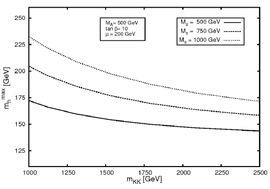
Figure 3.1: The variation of $m_{h}^{\rm max}$ with $m_{kk}$ for different choices of $M_{S}$. We have used $A_{u}=A_{d}=\sqrt{6}M_{S}$ to maximise the radiative effect.

3.3.4 Numerical Results

The scale of the extra dimension is best represented by the mass of the lightest KK particle. And as discussed in Section 3.2, the lightest particles are the members of the $N=2$ vector super fields and are given by Eq. 3.9. We denote this by $m_{kk}$, and all our results are plotted as a function of this variable.

In Figure 3.1, we have demonstrated that $m_{h}$ indeed falls with increasing $m_{kk}$, eventually attaining its 4d value. In this plot, we have set $A_{u}=A_{d}=\sqrt{6}M_{S}$, which maximizes not only the 4d MSSM radiative correction but also the KK-induced one, which is why we have used the symbol $m_{h}^{\rm max}$. The three lines correspond to three different choices of $M_{S}=$ 500, 750 and 1000 GeV. All in all, $m_{h}$ increases by a few to several tens of a GeV, depending on the choice of soft SUSY breaking parameters, the radiative contribution coming primarily from all up-type multiplets.

3.4 Conclusions

We have calculated one-loop correction to the lightest neutral Higgs boson mass in a generic MSSM embedded in a slice of AdS₅. For a reasonable choice of warped space parameters, the 4d upper limit of 135 GeV could be relaxed by as much as $\sim$ (50-100) GeV depending on $M_{S}$. A few other closely related highlights are the following: (i) matter KK spectra are controlled by the $c_{i}$ parameters, which, in turn, are determined by the zero mode fermion masses; (ii) all KK Yukawa couplings are close to unity to a very good approximation; (iii) the lightest KK states are the members of the $N=2$ vector supermultiplets; (iv) small values of $\tan\beta(\raisebox{-1.72218pt}{\hbox to0.0pt{$\sim$\hss}}\raisebox{1.72218pt}{$<$}~{}3)$, which are otherwise disfavored in 4d MSSM due to nonobservation of Higgs up to 114.5 GeV [113], are now resurrected thanks to an additional KK-induced radiative correction. Admittedly, the stability of the proton would require further care [77]. Besides, the warped models with fermions in the bulk, in general, pass the electroweak precision tests (EWPT) with some difficulty [96], unless the KK mass is raised to tens of a TeV. To suppress excessive contribution to $T$ (or $\Delta\rho$), gauge symmetry in the bulk is enhanced to ${\rm SU(2)_{L}\times SU(2)_{R}\times U(1)_{B-L}}$ [97], while, to keep the contributions to $Zb_{L}\bar{b}_{L}$ vertex and other loop corrections under control, a further discrete $L\leftrightarrow R$ symmetry has been employed [99]. This allows us to consider $m_{kk}$ as light as 1.5 TeV (i.e. KK gauge boson is of that order). Furthermore, $\tan\beta$ can be tuned to reduce the contribution to $T$. Since our primary intention here has been to develop a simple analytic framework (for the first time) to compute KK-induced radiative corrections to $m_{h}$ in a supersymmetric warped space, we pared the scenario down to its bare minimum. The further details necessary to overcome the above constraints are unlikely to alter the essential qualitative and quantitative features.

Chapter 4 A phenomenological study of 5d supersymmetry

4.1 Introduction

The CERN Large Hadron Collider (LHC) is all set to search out the yet elusive Higgs boson. But, LHC is also expected to reveal a new ruler of the tera-electron-volt (TeV) territories. The standard model (SM) has so far been remarkably successful in explaining physics up to a few hundred GeV energy scale. But theoretical inconsistencies of the SM (like, gauge hierarchy problem) and experimental requirements (like, a candidate to account for the dark matter of the universe) suggest that there are good reasons to believe that new physics beyond the SM is just around the corner crying out for verification. Among the different possibilities, supersymmetry and extra dimension stand out as the two leading candidates for dictating terms in the TeV regime. These two apparently distinct classes of scenarios cover a wide variety of more specific models. The usual practice from a bottom-up approach is to attach an ‘either/or’ tag on supersymmetry and extra dimension, as if the presence of one excludes the other. A more careful thought would reveal that the relationship between these two is not necessarily mutually exclusive. In fact, the presence of higher dimensions is a common feature of any fundamental theory valid at high scale. We will get back to this issue a little later. For the moment, to put things into perspective, we recapitulate the chronological evolution of the extra dimensional scenarios without invoking supersymmetry a priori. We restrict our discussion to the flat space scenarios, as we are not pursuing the warped path in this chapter.

Flat extra dimensions were first studied [55] in a scenario where gravity propagates in a millimeter (mm) size compact space dimension, with the SM particles confined to a 4d brane. The motive was to bring down the fundamental Planck scale to about a TeV. Subsequently, it was conceived that the brane where the SM particles live may actually have a very small size, like $10^{-16}$ cm $\sim{\rm TeV}^{-1}$, leading to the concept of a ‘fat brane’ [114]. In the context of the present chapter, we stick to the fat brane scenario. What are the experimental bounds on the fatness of such a brane, more precisely, on the radius of compactification ($R$)? For universal extra dimension (UED) models [115], in which all the SM particles access the extra dimensional bulk, a safe estimate is $R^{-1}~{}\raisebox{-1.72218pt}{\hbox to0.0pt{$\sim$\hss}}\raisebox{1.72218pt}{$>$}~{}500$ GeV. More specifically, the $g-2$ of the muon [116], flavor changing neutral currents [117, 119, 118], $Z\to b\bar{b}$ decay [120], the $\rho$ parameter [115, 121], and hadron collider studies [122] reveal that $R^{-1}~{}\raisebox{-1.72218pt}{\hbox to0.0pt{$\sim$\hss}}\raisebox{1.72218pt}{$>$}~{}300$ GeV. Consideration of $b\to s\gamma$, however, implies a somewhat tighter bound ($R^{-1}~{}\raisebox{-1.72218pt}{\hbox to0.0pt{$\sim$\hss}}\raisebox{1.72218pt}{$>$}~{}600$ GeV [123]). Methods to decipher its signals from the LHC data have recently been discussed too [124]. On the other hand, in the non-universal scenario where both the SM gauge bosons and the Higgs boson propagate in the bulk but the fermions are confined to a 4d brane [125], $R^{-1}$ cannot be below $(1-2)$ TeV [126]. The reason behind the difference in constraints is the following. The KK parity, defined by $(-1)^{n}$ for the $n$th KK label, is conserved in UED, while it is not a good symmetry in the non-universal scenario. As a result, while in the non-universal models KK states can mediate many processes at tree level yielding strong constraints, in the UED model, thanks to the KK parity, KK states appear only inside a loop leading to milder constraints. In any case, in the presence of supersymmetry, all those analyses need to be modified with more parameters, which would expectedly lead to a set of more relaxed bounds on $R^{-1}$.

The motivation of studying a TeV scale (or, a fat brane) extra dimension scenario has been investigated from the perspective of string theory, phenomenology, cosmology/astrophysics and high energy experiments. Such models provide a cosmologically stable dark matter candidate [127], trigger successful electroweak symmetry breaking successfully through a composite Higgs [128], address the fermion mass hierarchy problem from a different point of view [129], and stimulate power law renormalization group (RG) running yielding a lower (few tens of a TeV) gauge coupling (near-)unification scale [131, 132, 133]. Besides, the running of neutrino mixing angles generated from effective Majorana mass operator in a 5d set-up has been studied in both non-supersymmetric [135] and supersymmetric [136] contexts.

We argue that supersymmetry and extra dimension need not always be seen as two new physics considered simultaneously. In fact, they may nicely complement each other in some situations through mutual requirements. From a top-down approach, string theory provides a rationale behind linking supersymmetry and extra dimension. The string models are intrinsically extra dimensional, and more often than not contain supersymmetry as an integral part. That said, we must also admit that establishing a rigorous connection between a realistic low energy supersymmetric model with string theory is still a long shot, though a lot of efforts have already been put in that direction [137]. Even after embedding the SM in an extra dimensional set-up, the scalar potential remains unstable under quantum correction. Supersymmetrization stabilizes it and ameliorates the hierarchy problem. It is interesting to note that by admitting chiral fermions and their scalar partners in the same multiplet tacitly provides a rationale behind treating the Higgs boson as an elementary object. An elementary Higgs can be perfectly accommodated in a flat extra dimensional set-up. As a corollary, the upper limit on the lightest supersymmetric neutral Higgs is relaxed beyond the 4d upper limit of 135 GeV due to the presence of the KK towers of top/stop chiral multiplets, and the hitherto disfavored low $\tan\beta$ region can be resurrected [112]. Finally, each 4d supersymmetric scenario has its own supersymmetry breaking mechanism. The origin of this mechanism may be linked to the existence of extra dimension. In fact, one of the earliest motivations of a TeV scale fat brane was to relate the scale of 4d supersymmetry breaking with $R^{-1}$ [114, 138].

Keeping these in mind, we outline the formalism of a 5d supersymmetric model in an $S^{1}/Z_{2}$ orbifold which contains the 4d supersymmetric states as zero modes. In section 4.2, we state our assumptions leading to the construction of the 5d model and comment on supersymmetry breaking. Furthermore, we explicitly write down the particle content and their 5d Lagrangian and illustrate the KK decompositions of the different 5d fields. In section 4.3, we derive the beta functions of the gauge and Yukawa couplings as well as those of the different soft supersymmetry breaking parameters diagram by diagram, pointing out how they are all modified from their 4d values due to the presence of KK states. In section 4.4, we discuss the numerical effects of RG running and highlight the reason behind the differences between the 4d and 5d scenarios. We also point out under what conditions we can ensure electroweak symmetry breaking. In section 4.5, we exhibit the numerical impact of RG running through plots showing constraints in the $m_{0}$–$M_{1/2}$ plane. We standardize our numerical codes by reproducing the known 4d plots before encoding the necessary alterations for producing the new plots pertaining to 5d supersymmetry. This also enables us to compare and contrast the 4d and 5d allowed regions. Finally, in section 4.6, we showcase the essential features we have learnt from this analysis.

This rest of this chapter closely follows the work published in the paper:  G. Bhattacharyya and T. S. Ray, “A phenomenological study of 5d supersymmetry,”JHEP 1005 (2010) 040 [arXiv:1003.1276 [hep-ph]].

4.2 5d supersymmetry

4.2.1 A brief summary of our model

We highlight the salient features of supersymmetry in higher dimension and outline below the various assumptions that lead to a calculable phenomenological framework.

We consider a 5d flat space time metric. The 5th dimension is compactified on a $S_{1}/Z_{2}$ orbifold. Orbifolding is necessary to reproduce chiral zero mode fermions as a 5d theory is vector-like. We embed the minimal supersymmetric standard model (MSSM) in this higher dimensional set-up (several consequences of such embedding, mainly the effects on gauge and Yukawa couplings’ evolution, have been studied in [131]). From a 4d point of view, this leads to a tower of KK states. The massless sector corresponds to the 4d MSSM states. Since in 5d bulk the fermion representation is vectorial, the two-component spinor $Q$ that generates 4d supersymmetry will in 5d be accompanied by its chiral conjugate mirror $Q^{c}$. Thus a $N=1$ supersymmetry in 5d corresponds to two different $N=1$ supersymmetry, or equivalently, a $N=2$ supersymmetry from a 4d perspective. In fact, all the KK modes of a given level must fall into a valid representation of $N=2$ supersymmetry. In fact, each 4d supermultiplet is augmented by new chiral conjugate states and together they form a hypermultiplet. Here we are talking about a massive representation of supersymmetry, where the supersymmetry preserving Dirac mass plays the rôle of central charge for $N=2$ supersymmetry. This charge is not renormalized, as a consequence of which the bulk hypermultiplets do not receive any wave-function renormalization [131, 140]. We observe that this $N=2$ non-renormalization has serious numerical consequences in RG evolution of parameters. The most notable effect is the blowing up of the Yukawa couplings into the non-perturbative regime around 18 TeV, which we will take to be the cutoff of our theory. This is below the scale of perturbative gauge coupling unification, which is around 30 TeV. Recall that in 5d we encounter power law running which results in early (compared to 4d) unification.

We allow the gauge and the Higgs multiplets access the 5d bulk. Thus far what we said is nothing but a supersymmetrization of UED. Only the matter multiplets make the difference. In the UED framework, all SM particles access the bulk, and thus even though there are two fixed points, there is no brane. One could as well have kept some or all of the fermion generations in a brane at a fixed point; the difference would be that the scenario would cease to be universal. In the present supersymmetric context too we have the freedom of keeping some or all of the matter multiplets at an orbifold fixed point. We note that unless we confine at least two generations of matter multiplets on a brane, the requirement of perturbative gauge coupling unification leads to a constraint $R^{-1}>10^{10}$ GeV [133], spoiling its relevance for LHC. On the other hand, unless we keep the third family of matter multiplet in the bulk we cannot ensure electroweak breaking. In view of the above, we let the third generation matter multiplet access the bulk, but fix the first two generations at $y=0$. $N=2$ supersymmetry forbids Yukawa interaction in the 5d bulk as this interaction involves odd (three) number of chiral multiplets. Therefore, we localize Yukawa interaction at the orbifold fixed point where the supersymmetry corresponds to $N=1$.

Now we come to the important question as how we break the residual $N=1$ supersymmetry. Different ideas have been advanced for its realization. One way is to break it by the Scherk-Schwarz mechanism [141] in which fermions and bosons satisfy different periodic conditions over the compactified dimension. Explicit realizations towards this using a TeV-scale orbifold can be found in [142]. Another interesting approach was to break the residual supersymmetry by a second compactification on an orbifold with two reflection symmetries, viz. $S^{1}/(Z_{2}\times Z_{2}^{\prime})$ [143]. This can be viewed as a discrete version of the Scherk-Schwarz mechanism. Both these scenarios yield soft masses which are UV insensitive due to the non-local nature of supersymmetry breaking. From a completely different viewpoint, supersymmetry breaking may be infused from the brane-bulk interface [144], or transmitted from a distant brane [150], or arisen from a gaugino mediation set-up [145] (possibly with a much lower cutoff than $10^{16}$ GeV), or triggered by some completely unknown brane dynamics, for example, by a spurion $F$-term vacuum expectation value (vev). In the context of the present analysis, we keep the exact mechanism of the $N=1$ brane supersymmetry breaking unspecified. We assume that the supersymmetry breaking scale is of the order of the inverse of radius of compactification, for example $c/R$, where $c$ is an ${\cal{O}}(1)$ dimensionless parameter.

Our main goal is the following: Just like in the conventional but constrained version of 4d supersymmetry one starts with a common scalar and a common gaugino mass at high scale (e.g. the GUT scale) and then run them down using the MSSM beta functions to find the weak scale spectrum, we do exactly the same here by assuming a common scalar mass ($m_{0}$) and a common gaugino mass ($M_{1/2}$) at low cutoff scale (18 TeV) and follow the running using the KK beta functions through successive KK thresholds to obtain the weak scale parameters. By adopting a phenomenological approach, we scan $m_{0}$ and $M_{1/2}$ over a set of values $c/R$, with $c$ varying in the range $0.1$ to $1$ and $R^{-1}$ fixed at $1$ TeV.

4.2.2 Multiplet Structures

As mentioned in the introduction, from a 4d perspective, the KK towers of matter and gauge fields rearrange in the form of $N=2$ hypermultiplets. A judicious choice of $Z_{2}$ parity of the 5d fields allows us to break the $N=2$ supersymmetry to $N=1$ supersymmetry. We briefly review below the multiplet structures of the fields following the prescription suggested in [108].

Vector hypermultiplet

The 5d super Yang-Mills theory contains a 5-vector gauge field, a 4-component Dirac gaugino and a real scalar. When dimensionally reduced to 4d, the gauge field splits into a 4-vector and a scalar, the gaugino splits into 2 Majorana gauginos, and we still have the real scalar previously mentioned. All these fit into a vector multiplet and a chiral multiplet in $N=1$ language. If we represent the $N=2$ vector supermultiplet by $V$, the 4-vector gauge field by $A_{\mu}$, the gauginos by $\lambda$ and $\psi$, and define a complex scalar field $\phi\equiv\frac{1}{2}(\Sigma+iA_{5})$, where $\Sigma$ is the 5d real scalar and $A_{5}$ is the 5th component of the 5-vector field, then one can schematically represent the 5d vector supermultiplet as

$$V\equiv\pmatrix{A_{\mu}&\phi\cr\lambda&\psi\cr}\,.$$ (4.1)

From a 4d perspective (where the compactified 5th coordinate $y$ is just a label), and in the $N=1$ language, one can visualize the vector hypermultiplet by a vector multiplet $\mathcal{V}$ (first column) and a chiral multiplet in the adjoint representation by $\Phi$ (second column):

$${\mathcal{V}}(x,y) = -\theta{\sigma}^{\mu}\overline{\theta}A_{\mu}{(x,y)}+i~{}{\overline{\theta}}^{2}\theta{\lambda}{(x,y)}-i~{}{\theta}^{2}\overline{\theta}~{}{\overline{\lambda}}{(x,y)}+\frac{1}{2}{\overline{\theta}}^{2}{\theta}^{2}D_{V}(x,y)\,,$$

$${\Phi}{(x,y)} = {\phi}{(x,y)}+\sqrt{2}~{}\theta{\psi}{(x,y)}+{\theta}^{2}F_{\Phi}(x,y)\,.$$ (4.2)

The $Z_{2}$ parity of $V$ is so chosen that the $\mathcal{V}$ contains a zero mode, but $\Phi$ does not have any zero mode.

The gauge invariant action may be written as ($\int d^{5}x\equiv\int d^{4}x\int dy$)

$$S^{5}_{\rm gauge}=\int d^{5}x\left[\frac{1}{4g^{2}}\int d^{2}\theta~{}W^{\alpha}W_{\alpha}+{\rm h.c.}+\int d^{4}\theta~{}\frac{1}{g^{2}}{\left({\partial}_{5}\mathcal{V}-\frac{1}{\sqrt{2}}\left(\Phi+\overline{\Phi}\right)\right)}^{2}\right],$$ (4.3)

where the $~{}W^{\alpha}(x,y)$ is the field strength superfield corresponding to ${\mathcal{V}}(x,y)$.

Higgs hypermultiplets

From the $N=1$ perspective, the $N=2$ hypermultiplet splits into two chiral multiplets. Thus we have a $H_{u}$ hypermultiplet and a $H_{d}$ hypermultiplet. We can represent them as (the tilde symbol represents Higgsino)

$${H_{(u,d)}}\equiv\pmatrix{{H_{L(u,d)}}&{H_{R(u,d)}}\cr{\tilde{H}_{L(u/d)}}&{\tilde{H}_{R(u/d)}}\cr}\,.$$ (4.4)

If we denote the two chiral multiplets inside the hypermultiplet $H(x,y)$ as $h(x,y)$ in left column and $h^{c}(x,y)$ in right column, then one can expand the chiral superfield as

$${h/h^{c}}={H_{L/R}}+\sqrt{2}~{}\theta{\tilde{H}_{L,R}}+{\theta}^{2}F_{h/h^{c}}\,.$$ (4.5)

We assign even $Z_{2}$ parity to $h$ so that it has a zero mode, and odd $Z_{2}$ parity to $h^{c}$ which does not have zero mode. The free action of the hypermultiplets can be written as

$$S^{5}_{\rm Higgs}=\int d^{5}x\left[\int d^{4}\theta\left({\overline{h}}^{c}h^{c}+{\overline{h}}h\right)+\left(\int d^{2}\theta~{}h^{c}\left({\partial}_{5}+m\right)h+{\rm h.c.}\right)\right]\,.$$ (4.6)

Matter hypermultiplets

Matters have hypermultiplet structures similar to Higgs:

$$\Psi\equiv\pmatrix{{{\phi}_{L}}&{{\phi}_{R}}\cr{{\psi}_{L}}&{{\psi}_{R}}\cr}~{},$$ (4.7)

where, ${{\mathcal{F}}_{L}}\equiv\left({{\phi}_{L}},{{\psi}_{L}}\right)$ ($Z_{2}$ even) and ${{\mathcal{F}}_{R}}\equiv\left({{\phi}_{R}},{{\psi}_{R}}\right)$ ($Z_{2}$ odd) represent the two $N=1$ chiral multiplets. The free matter hypermultiplet action will be similar to Eq. 4.6. There are five matter representations, two SU(2) doublets $Q$ and $L$ and three singlets $u,d,e$, where the symbols have their standard meaning.

Gauge interactions

When the hypermultiplets are charged under gauge symmetry, their free action can be promoted to take care of the interaction in the following way:

$$S^{5}_{\rm int} = \int d^{5}x\left[\int d^{4}\theta\left({{\mathcal{F}}_{L}}e^{\mathcal{V}}{{\overline{\mathcal{F}}}_{L}}+{{\mathcal{F}}_{R}}e^{-{\mathcal{V}}}{{\overline{\mathcal{F}}}_{R}}\right)+\left\{\int d^{2}\theta{\mathcal{F}}_{L}\left(m+{\partial}_{5}-\frac{1}{\sqrt{2}}{\Phi}\right){{\mathcal{F}}_{R}}+{\rm h.c.}\right\}\right]$$ (4.8)

where, ${\mathcal{V}}={\mathcal{V}}^{a}T^{a}$ and ${\Phi}={\Phi}^{a}T^{a}$ are Lie-algebra-valued gauge and matter superfields.

Yukawa Interactions

Since Yukawa interaction involves three (i.e. odd number) chiral superfields, it is not possible to write a bulk Yukawa interaction maintaining $N=2$ supersymmetry. For this reason, we confine Yukawa interaction at the branes. We denote the Yukawa part of the superpotential by $W_{Y}$, which contains the usual chiral superfield combinations $QH_{u}u$, $QH_{d}d$ and $LH_{d}e$. Then the action can be written as

$$S^{5}_{\rm Yuk}=\int d^{5}x\left(\int d^{2}\theta~{}W_{Y}\right)\left[\delta(y)+\delta(y-{\pi}R)\right]\,.$$ (4.9)

As the $Z_{2}$ odd fields vanish at the fixed points, they do not contribute to Yukawa interactions.

4.2.3 KK decomposition of fields

In order to obtain the action in terms of 4d component fields, we need to write down the KK decomposition of the 5d fields in terms of zero modes and higher KK modes [115]. Each 5d field is either $Z_{2}$ even or $Z_{2}$ odd. Only the even fields have zero modes. The decomposition of the Higgs fields will be exactly like the matter fields.

$$\mathcal{V}(x,y) = \frac{\sqrt{2}}{\sqrt{2\pi R}}\mathcal{V}^{(0)}(x)+\frac{2}{\sqrt{2\pi R}}\sum^{\infty}_{n=1}\mathcal{V}^{(n)}(x)\cos\frac{ny}{R}\,,$$

$$\Phi(x,y) = \frac{2}{\sqrt{2\pi R}}\sum^{\infty}_{n=1}\Phi^{(n)}(x)\sin\frac{ny}{R}\,,$$ (4.10)

$${\mathcal{F}}_{L}(x,y) = \frac{\sqrt{2}}{\sqrt{2\pi R}}{\mathcal{F}}_{L}^{(0)}(x)+\frac{2}{\sqrt{2\pi R}}\sum^{\infty}_{n=1}{\mathcal{F}}_{L}^{(n)}(x)\cos\frac{ny}{R}\,,$$

$${\mathcal{F}}_{R}(x,y) = \frac{2}{\sqrt{2\pi R}}\sum^{\infty}_{n=1}{\mathcal{F}}_{R}^{(n)}(x)\sin\frac{ny}{R}\,.$$

4.3 RG evolution and derivation of the beta functions

The technical meaning of RG evolution in a higher dimensional context has been amply clarified in [131], and we merely reiterate it in the present context. The multiplicity of KK states renders any such higher dimensional scenario non-renormalizable. So ‘running’ of couplings or parameters with the energy scale does not make much of a sense. Rather, one can estimate the finite quantum corrections that these couplings/parameters receive whose size depends on some explicit cutoff $\Lambda$. The contribution comes from $\Lambda R$ number of KK states which lie between the scale of the first KK state, which is $1/R$, and the cutoff $\Lambda$. With this interpretation of RG running, we compute the one loop beta functions of the gauge and Yukawa couplings and various soft supersymmetry breaking masses. We make the following observations:

1. The contribution to the beta function from a given KK mode does not depend on its KK label.

2. When we consider different KK thresholds we neglect their zero mode masses, i.e. we assume that the $n$th level KK state is kicked into life when we cross the energy scale $n/R$.

3. As we cross different KK thresholds, the beta functions also change. The beta function of the quantity $X$ at an energy scale $Q$, where $n~{}\raisebox{-1.72218pt}{\hbox to0.0pt{$\sim$\hss}}\raisebox{1.72218pt}{$<$}~{}QR<(n+1)$, can be written as ($t=\ln(Q/Q_{0})$, where $Q_{0}$ is a reference scale, e.g. the electroweak scale)

   $$\frac{\partial{X}}{\partial{t}}=\beta_{X}\,,~{}~{}{\rm where}~{}~{}\beta_{X}=\beta_{0X}+n\tilde{\beta}_{X}\,.$$ (4.11)

   Here $\beta_{0X}$ is the contribution induced by the zero mode (i.e. ordinary 4d MSSM) states (which may be found, for example, in the review [54]) and $\tilde{\beta}_{X}$ arises from a single KK mode. Eq. 4.11 is our master equation, using which we perform a diagram by diagram calculation for the estimation of $\tilde{\beta}_{X}$ for various couplings and parameters.

4.3.1 Gauge couplings and gaugino masses

The running of the gauge couplings ($g_{i}$) and gaugino masses ($M_{i}$) are controlled by

$$\beta_{g_{i}}=\frac{g_{i}^{3}}{16\pi^{2}}\left[b_{i}^{0}+n\tilde{b}_{i}\right]\,,~{}~{}\beta_{M_{i}}=\frac{g_{i}^{2}M_{i}}{16\pi^{2}}\left[b_{i}^{0}+n\tilde{b}_{i}\right]\,.$$ (4.12)

For the gauge groups U(1) (which corresponds to $g_{1}=\sqrt{5/3}g^{\prime}$, which unifies), SU(2) and SU(3), $b_{i}^{0}=(33/5,1,-3)$, and $\tilde{b}_{i}=(26/5,2,-2)$ respectively.

4.3.2 Yukawa and scalar trilinear couplings

We recall that $N=1$ non-renormalization relates the beta functions of the Yukawa couplings ($y_{ijk}$) to the anomalous dimension matrices ($\gamma^{i}_{j}$) of the superfields. This theorem implies that logarithmically divergent contributions can always be written in terms of wave-function renormalizations. Generically, $y_{ijk}$ may be written as

$$\beta_{y^{ijk}}=\gamma^{i}_{n}y^{njk}+\gamma^{j}_{n}y^{ink}+\gamma^{k}_{n}y^{ijn}\,.$$ (4.13)

The Feynman diagrams showing the KK contributions to the wave-function renormalizations of the scalars and fermions are displayed in Figure 4.1. The contribution from the gauge sector cancels exactly as a consequence of the $N=2$ non-renormalization theorem mentioned in section 4.2. Diagrammatically, the origin of this cancellation may be traced to a relative sign between the $A_{\mu}$- and $\phi$-propagators - see Eq. 4.1. Only the brane localized Yukawa interactions contribute to the Yukawa evolution. We also keep track of the fact that the $\mathbb{Z}_{2}$ odd fields have vanishing wave-functions at the two branes, leaving the even fields alone to contribute to the diagrams in Figure 4.1. Here we have made a tacit assumption that although the Yukawa interaction is brane localized, only one KK level ($n$) states float inside the loop at a time. This is a technical assumption to ensure calculability by avoiding KK divergence which would have arisen while summing more than one KK index in a loop calculation.

Figure 4.1: Feynman diagrams showing the KK contributions to the wave-function renormalizations of the zero mode $u_{3}$ and $H_{u}$. Similar diagrams for the other fermions and scalars may be drawn analogously. Here $A_{\mu}$ is a generic gauge field and $\phi$ is an adjoint scalar, both arising from a vector hypermultiplet.

To appreciate the numerical impact of the bulk $N=2$ non-renormalization, we first write down the conventional 4d MSSM beta functions (i.e. those coming from zero mode states in the 5d context) which contribute to the evolution of the third generation Yukawa couplings [54]:

$$\beta_{t}^{0} = {y_{t}\over 16\pi^{2}}\Bigl{[}6y_{t}^{*}y_{t}+y_{b}^{*}y_{b}-{16\over 3}g_{3}^{2}-3g_{2}^{2}-{13\over 15}g_{1}^{2}\Bigr{]},$$

$$\beta_{b}^{0} = {y_{b}\over 16\pi^{2}}\Bigl{[}6y_{b}^{*}y_{b}+y_{t}^{*}y_{t}+y_{\tau}^{*}y_{\tau}-{16\over 3}g_{3}^{2}-3g_{2}^{2}-{7\over 15}g_{1}^{2}\Bigr{]}\,,$$ (4.14)

$$\beta_{\tau}^{0} = {y_{\tau}\over 16\pi^{2}}\Bigl{[}4y_{\tau}^{*}y_{\tau}+3y_{b}^{*}y_{b}-3g_{2}^{2}-{9\over 5}g_{1}^{2}\Bigr{]}\,.$$

The corresponding KK contributions are given by

$$\tilde{\beta}_{f}=\beta_{f}^{0}(g_{i}\to 0)~{}~{}(f\equiv t,b,\tau)\,,$$ (4.15)

where the vanishing gauge contributions are a direct consequence of the bulk $N=2$ non-renormalization.

The effects of the above non-renormalization can also be felt in the evolution of the trilinear scalar couplings. The relevant Feynman diagrams are displayed in Figure 4.2. Again, for illustration, we first write down the contributions to the beta functions from the zero mode (i.e. 4d MSSM) states [54]:

$${\beta}_{a_{t}}^{0}\! = \!\frac{1}{16\pi^{2}}\Bigl{[}a_{t}\left(18y_{t}^{*}y_{t}+y_{b}^{*}y_{b}-{16\over 3}g_{3}^{2}-3g_{2}^{2}-{13\over 15}g_{1}^{2}\right)+2a_{b}y_{b}^{*}y_{t}\Bigr{.}$$

$$\!+~{}y_{t}\Bigl{.}\left({32\over 3}g_{3}^{2}M_{3}+6g_{2}^{2}M_{2}+{26\over 15}g_{1}^{2}M_{1}\right)\Bigr{]}\,,$$

$${\beta}_{a_{b}}^{0}\! = \!\frac{1}{16\pi^{2}}\Bigl{[}a_{b}\left(18y_{b}^{*}y_{b}+y_{t}^{*}y_{t}+y_{\tau}^{*}y_{\tau}-{16\over 3}g_{3}^{2}-3g_{2}^{2}-{7\over 15}g_{1}^{2}\right)+2a_{t}y_{t}^{*}y_{b}+2a_{\tau}y_{\tau}^{*}y_{b}\Bigr{.}\phantom{xxxx}$$ (4.16)

$$\!+y_{b}\Bigl{.}\left({32\over 3}g_{3}^{2}M_{3}+6g_{2}^{2}M_{2}+{14\over 15}g_{1}^{2}M_{1}\right)\Bigr{]}\,,\qquad{}$$

$$\beta_{a_{\tau}}^{0}\! = \!\frac{1}{16\pi^{2}}\Bigl{[}a_{\tau}\left(12y_{\tau}^{*}y_{\tau}+3y_{b}^{*}y_{b}-3g_{2}^{2}-{9\over 5}g_{1}^{2}\right)+6a_{b}y_{b}^{*}y_{\tau}+y_{\tau}\left(6g_{2}^{2}M_{2}+{18\over 5}g_{1}^{2}M_{1}\right)\Bigr{]}\,.$$

As expected, the beta functions of the soft supersymmetry breaking parameters are proportional not only to those parameters but to others as well, since any non-renormalization theorem ceases to work when supersymmetry is broken. For the computation of $\tilde{\beta}_{a_{f}}$, we need to keep in mind the essence of Eq. 4.15, i.e. the absence of gauge contributions in $\tilde{\beta}_{f}$, while solving the coupled differential equations. However, that part of the gauge contributions (proportional to $g_{i}^{2}$) to the trilinear scalar couplings which multiply the gaugino masses ($M_{i}$) in Eq. 4.3.2 would still remain while computing the KK contribution. All in all,

$$\tilde{\beta}_{a_{f}}=\beta_{a_{f}}^{0}(a_{f}g_{i}\to 0)\,.$$ (4.17)

Figure 4.2: Feynman diagrams showing the KK loop contribution to the evolution of a trilinear scalar coupling. The diagrams contributing to other trilinear couplings may be drawn analogously.

4.3.3 Scalar masses

We make three observations regarding the KK contributions to the evolution of scalar masses (see Figure 4.3):

1. The two diagrams in the lower row of Figure 4.3 depend on the Yukawa couplings. Hence, they are important only for the third generation matter fields.

2. Recall that in the evolution of the Yukawa couplings the KK contributions from the gauge field $A_{\mu}$ and the complex scalar $\phi$ exactly cancelled thanks to the bulk $N=2$ non-renormalization. However, their fermionic superpartners contribute to the scalar mass evolution and those contributions add up instead of canceling out. This happens because these contributions yield gaugino masses which are $N=1$ supersymmetry breaking parameters and hence the non-renormalization theorem ceases to be applicable.

3. Each KK state in the two diagrams in the top row of Figure 4.3 contributes twice that of the SM because of the doubling of the fermions (this factor of 2 is highlighted in bold-face in Eqs. 4.3.3 and 4.3.3 below). However, each KK state at the lower row diagrams contributes the same as in the SM because the odd fermion modes vanish at the brane where Yukawa interaction is confined.

Below we write down the beta functions of the third generation scalars:

$$\tilde{\beta}_{u_{3}} = \frac{1}{16\pi^{2}}\left[2\left(2y_{t}^{2}\left(m_{Hu}^{2}+m_{\tilde{Q}_{3}}^{2}+m_{\tilde{u}_{3}}^{2}\right)+2a_{t}^{2}\right)\right.-\left.{\bf 2}\left(\frac{32}{3}g_{3}^{2}|M_{3}|^{2}+\frac{32}{15}g_{1}^{2}|M_{1}|^{2}+\frac{4}{5}g_{1}^{2}S\right)\right],$$

$$\tilde{\beta}_{d_{3}} = \frac{1}{16\pi^{2}}\left[2\left(2y_{b}^{2}\left(m_{Hd}^{2}+m_{\tilde{Q}_{3}}^{2}+m_{\tilde{d}_{3}}^{2}\right)+2a_{b}^{2}\right)\right.-\left.{\bf 2}\left(\frac{32}{3}g_{3}^{2}|M_{3}|^{2}+\frac{8}{15}g_{1}^{2}|M_{1}|^{2}-\frac{2}{5}g_{1}^{2}S\right)\right],$$

$$\tilde{\beta}_{Q_{3}} = \frac{1}{16\pi^{2}}\left[\left(2y_{t}^{2}\left(m_{Hu}^{2}+m_{\tilde{Q}_{3}}^{2}+m_{\tilde{u}_{3}}^{2}\right)+2a_{t}^{2}\right)\right.+\left.\left(2y_{b}^{2}\left(m_{Hd}^{2}+m_{\tilde{Q}_{3}}^{2}+m_{\tilde{d}_{3}}^{2}\right)+2a_{b}^{2}\right)\right.$$ (4.18)

$$\left.-{\bf 2}\left(\frac{32}{3}g_{3}^{2}|M_{3}|^{2}+6g_{2}^{2}|M_{2}|^{2}+\frac{2}{15}g_{1}^{2}|M_{1}|^{2}-\frac{1}{5}g_{1}^{2}S\right)\right],$$

$$\tilde{\beta}_{L_{3}} = \frac{1}{16\pi^{2}}\left[\left(2y_{\tau}^{2}\left(m_{Hd}^{2}+m_{\tilde{L}_{3}}^{2}+m_{\tilde{e}_{3}}^{2}\right)+2a_{\tau}^{2}\right)-{\bf 2}\left(\frac{6}{5}g_{1}^{2}|M_{1}|^{2}+\frac{3}{5}g_{1}^{2}S\right)\right],$$

$$\tilde{\beta}_{e_{3}} = \frac{1}{16\pi^{2}}\left[2\left(2y_{\tau}^{2}\left(m_{Hd}^{2}+m_{\tilde{L}_{3}}^{2}+m_{\tilde{e}_{3}}^{2}\right)+2a_{\tau}^{2}\right)-{\bf 2}\left(\frac{24}{5}g_{1}^{2}|M_{1}|^{2}-\frac{6}{5}g_{1}^{2}S\right)\right]\,.$$

The beta functions for the Higgs scalars are given by

$${\beta}_{H_{u}} = \frac{1}{16\pi^{2}}\left[3\left(2y_{t}^{2}\left(m_{Hu}^{2}+m_{\tilde{Q}_{3}}^{2}+m_{\tilde{u}_{3}}^{2}\right)+2a_{t}^{2}\right)\right.-\left.{\bf 2}\left(6g_{2}^{2}|M_{2}|^{2}+\frac{6}{5}g_{1}^{2}|M_{1}|^{2}-\frac{3}{5}g_{1}^{2}S\right)\right]\,,$$

$${\beta}_{H_{d}} = \frac{1}{16\pi^{2}}\left[3\left(2y_{b}^{2}\left(m_{Hd}^{2}+m_{\tilde{Q}_{3}}^{2}+m_{\tilde{d}_{3}}^{2}\right)+2a_{b}^{2}\right)\right.+\left(2y_{\tau}^{2}\left(m_{Hd}^{2}+m_{\tilde{L}_{3}}^{2}+m_{\tilde{e}_{3}}^{2}\right)+2a_{\tau}^{2}\right)$$

$$-\left.{\bf 2}\left(6g_{2}^{2}|M_{2}|^{2}+\frac{6}{5}g_{1}^{2}|M_{1}|^{2}+\frac{3}{5}g_{1}^{2}S\right)\right]\,.$$

Figure 4.3: Feynman diagrams showing the KK contributions to the running of the up-type Higgs mass. Diagrams contributing to the evolution of the other soft scalar masses may be drawn analogously.

4.4 Special numerical features of RG running in 5d scenario

In this section, we highlight the special features of RG evolution in the 5d scenario. We also compare and contrast them with the 4d features. For all our numerical estimates we have fixed $1/R=1$ TeV.

4.4.1 The Gauge and Yukawa couplings

The power law running of the gauge and Yukawa couplings has been discussed in [131, 133] for the non-supersymmetric scenario and in [131] for the supersymmetric case. As far as the Higgs multiplets are concerned, there is a crucial difference between our model and that considered in [131]. In our scenario there are separate up- and down-type Higgs hypermultiplets - see Eq. 4.4. Inside each hypermultiplet only the left column with label ($L$) is $\mathbb{Z}_{2}$ even and its scalar zero mode receives a vev, whereas the right column with label ($R$) is projected out. In other words, the hypermultiplet $H_{u}$ contains the vev $v_{u}$ and, similarly, $H_{d}$ contains $v_{d}$. On the other hand, [131] contains a single hypermultiplet, each column of which has a zero mode, one to be identified with the up-type chiral multiplet which contains the vev $v_{u}$, and the other to be identified with the down-type containing $v_{d}$. While our approach constitutes a straightforward generalization of $H_{u}$ and $H_{d}$ from chiral multiplets to hypermultiplets, the choice made in [131] requires non-trivial boundary conditions. These two different assumptions lead to significant numerical differences. In our approach, the gauge couplings converge to one another but actually do not meet at a single point, while in [131] the gauge couplings do meet at a point. The difference in the number of KK scalar excitations makes the difference between the two approaches.

Indeed, both gauge and Yukawa couplings exhibit power law running due to summation over the KK states as one crosses the energy thresholds. As we have mentioned in section 4.2, keeping the first two matter generations confined at the brane ensures that the couplings remain perturbative even with $R^{-1}$ as low as 1 TeV. Starting from their LEP-measured values at the weak scale, as we extrapolate the gauge couplings using the KK beta functions we observe that the three couplings approach very close to one another near 32 TeV, but they do not actually meet at any point, as mentioned in the previous paragraph.

A crucial point of immense numerical significance is that on account of the special $N=2$ bulk non-renormalization, the third generation matter hypermultiplet kept in the bulk does not receive any wave-function renormalization from the gauge hypermultiplet, which we have illustrated below Eq. 4.13. As an important consequence of this, the Yukawa couplings blow up to large (non-perturbative) values around $\Lambda\sim$ 18 TeV, which we therefore take to be the effective cutoff of our theory.

4.4.2 The gaugino and scalar masses

We assume that at the highest scale $\Lambda=18$ TeV of our theory, i.e. just before the Yukawa couplings blow up, all scalar masses unify to $m_{0}$ and all gaugino masses to $M_{1/2}$. Our high scale parameters are then $m_{0},M_{1/2},\mbox{sgn}(\mu)$ and $\tan\beta\equiv v_{u}/v_{d}$.

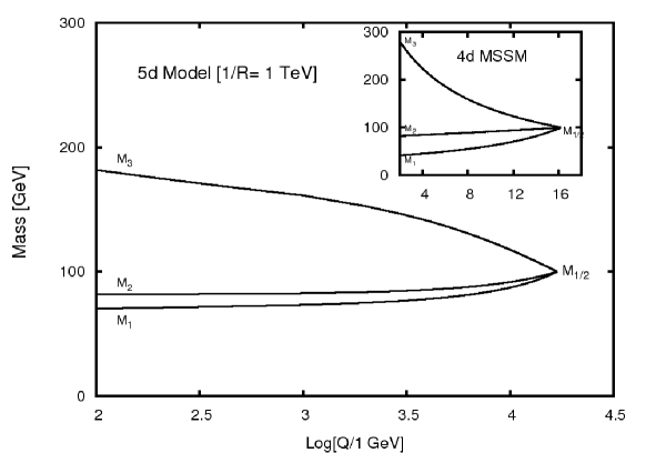
Figure 4.4: RG running of the gaugino masses.

The gaugino mass running is governed by the evolution of gauge couplings. Since gauge couplings nearly meet around 32 TeV, the gaugino masses tend to converge also at that scale. But in the present context, as mentioned before, we forced the gaugino masses to unify at 18 TeV. Recall that in 5d the running is short but fast (power law), but in 4d it is long and slow (logarithmic). This leads to a general expectation that, starting from a given high scale value, the low scale predictions would be similar in 4d and 5d. But since we forcibly unified the gaugino masses in our set-up, earlier than otherwise expected, we obtain a somewhat different set of low scale values. The gaugino mass scaling in 5d is shown in Figure 4.4, while in the inset, the 4d running is displayed. A rough comparison of the weak scale ratios of the three gaugino masses is presented below:

$$M_{1},M_{2},M_{3} \sim (0.4,0.8,3.0)\times M_{1/2}~{}\mbox{(in 4d)}\,,$$

$$M_{1},M_{2},M_{3} \sim (0.7,0.8,2.0)\times M_{1/2}~{}\mbox{(in 5d)}\,.$$ (4.20)

If $R$-parity remains conserved, the lightest neutralino remains the lightest supersymmetric particle (LSP), only that its mass is heavier than what is expected in the standard 4d scenario - see Eq. 4.20.

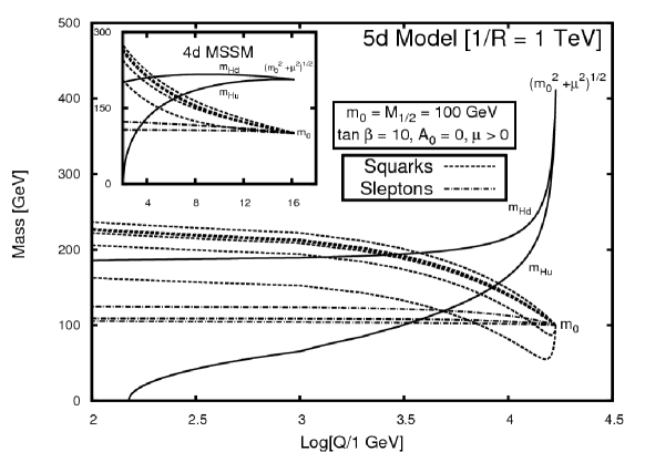
Figure 4.5: RG running of the scalar masses and radiative electroweak symmetry breaking.

Figure 4.5 shows the running of the soft scalar masses. The large top quark Yukawa coupling continues to play a crucial rôle as in 4d. A rough comparison of the weak scale predictions in 4d and 5d is:

$$m_{\tilde{Q}_{3}}^{2} \sim m_{0}^{2}+5.5M_{{1}/{2}}^{2}~{}\mbox{(in 4d)}\,,$$

$$m_{\tilde{Q}_{3}}^{2} \sim m_{0}^{2}+3.5M_{{1}/{2}}^{2}~{}\mbox{(in 5d).}$$ (4.21)

Even for the brane localized scalars, the 5d model predicts slightly higher weak scale masses compared to 4d.

During power law running we ensure that radiative breaking of electroweak symmetry does happen at the desired scale. Just like in 4d, only $m_{H_{u}}^{2}$ turns negative while all other scalars remain positive. Again, the large top quark Yukawa coupling drives this phase transition. A point to note is that unless we keep the third generation matter in the bulk, electroweak symmetry would never break radiatively in our class of models.

4.5 The $m_{0}-M_{1/2}$ parameter space

4.5.1 Numerical procedure

For our numerical estimates we go through the following steps:

1. We scan $m_{0}$ and $M_{1/2}$ over a range $[0.1-1.0]/R$. We choose $\tan\beta=10$ and take both positive and negative values of $\mu$. We use one loop RG equations as displayed in section 4.3.

2. For each input combination, we perform a consistency check to ensure correct electroweak symmetry breaking, and accept only those inputs which admit this phenomenon.

3. We then feed the weak scale spectrum into the code micrOMEGAS [147], and using this software package calculate the dark matter density ($\Omega_{\rm DM}$), ${\rm Br}~{}(b\rightarrow s\gamma)$, $\Delta a_{\mu}=(g-2)_{\mu}/2$, and $\Delta\rho$. Since we consider $1/R=1$ TeV, which is a bit too high compared to the lighter section of the zero mode superparticle spectrum, we neglect the direct loop contributions of the KK particles. In other words, the KK effects feed into the calculation of low energy spectra via power law running, but after that we rely on the standard 4d computations encoded in micrOMEGAS. This approximation is good enough for our purpose.

4. We compare the predictions of the above observables with their experimental values/constraints, and translate the information into the inclusion/exclusion plots, given in Figures 4.6 and 4.7 in the $m_{0}-M_{1/2}$ plane. The 4d plots have been reproduced to serve as a guide to the eyes for capturing the 5d subtleties. We note that our 4d plots are in agreement with the ones in the existing literature, e.g. with [148].

4.5.2 Comparison between 4d and 5d models

We highlight only the major differences between the 4d and 5d models that appear in the $m_{0}$–$M_{1/2}$ plane.

1. We assume that $R$-parity is conserved. In the 4d scenario the lightest neutralino is the most likely candidate for an LSP. In the 5d model the situation is somewhat tricky. Indeed, the 4d LSP is still an LSP here which is the zero mode neutralino. Besides, if the KK parity remains conserved, then the $n=1$ mode of photon tower, namely $\gamma_{1}$, and its supersymmetric partner $\tilde{\gamma}_{1}$ are also stable dark matter candidates. However, the KK parity is unlikely to be respected by the brane-bulk interaction. In our numerical analysis, we have treated the zero mode LSP as the dark matter candidate.

2. We have taken a $3\sigma$ range of the five year average of WMAP dark matter density ($0.087<\Omega_{\rm DM}h^{2}<0.138$) [33]. We raise a caution here that if KK parity remains conserved and we have two more dark matter candidates, as mentioned above, then the edge of the allowed band arising from the lower limit of $\Omega_{\rm DM}$ would be further stretched. Note further that in the 5d case there is a slight broadening of the WMAP allowed strip compared to 4d. This happens because of a combined effect of Eqs. 4.20 and 4.21 leading to a reduced sensitivity to $M_{1/2}$ variation.

3. As a consequence of Eq. 4.20, to arrive at a given value of $M_{1}$, one needs to start from a smaller $M_{1/2}$ in 5d compared to 4d. For this reason, the region where the lightest neutralino satisfies the dark matter constraints extends to a lower value of $M_{1/2}$ in 5d compared to 4d.

4. We have taken $2.65\times 10^{-4}\lesssim{\rm Br}~{}(b\to s\gamma)\lesssim 4.45\times 10^{-4}$ [149], and $10.6\times 10^{-10}\lesssim\Delta a_{\mu}^{\rm new}=(g-2)_{\mu}/2\lesssim 43.6\times 10^{-10}$ [30]. There is nothing much to distinguish between 4d and 5d from these two observables.

5. We have not included the direct loop effects of the virtual KK states for any of the weak scale observables. For $R^{-1}=1$ TeV or more, for processes like muon anomalous magnetic moment or $b\to s\gamma$, such effects are numerically negligible, but only for the Higgs mass it makes a difference. In Figures. 4.6 and 4.7, the entire region to the left of the line marked with $m_{h}=114$ GeV is disfavored from the non-observation of the Higgs boson. However, if we include the KK loop correction to the Higgs mass [112], the entire hitherto disfavored region is resurrected.

6. To ensure correct electroweak symmetry breaking, we had to take a factor 2 to 3 larger (than 4d) value of $\mu$ in 5d at the cutoff scale. Otherwise $m_{H_{u}}^{2}$ would become negative at a scale higher than required, thanks again to the bulk $N=2$ non-renormalization.

4.6 Conclusions and Outlook

We reiterate that the presence of extra dimensions is an essential part of any high scale fundamental theory, and supersymmetry is quite often an integral component of such theories. Furthermore, extra dimension may trigger supersymmetry breaking. Be it a Scherk-Schwarz mechanism, or a breaking triggered by a spurion $F$-term vev, or due to compactification on the orbifold $S^{1}/(\mathbb{Z}_{2}\times\mathbb{Z}_{2}^{\prime})$, or for that matter any top-down scenario that contains supersymmetry, would find a common ground in our phenomenological model where we varied $m_{0}$ and $M_{1/2}$ in a reasonable range $[0.1-1.0]R^{-1}$.

The logarithmic running in 4d from 100 GeV to $10^{16}$ GeV is replaced in 5d by fast power law running on a shorter interval from 100 GeV to about 30 TeV in 5d thanks to the KK states. This has nothing to do with supersymmetry. What is special about 5d supersymmetry is a special $N=2$ non-renormalization that forces us to consider an early cutoff ($\sim$ 18 TeV).

The constraints in the $m_{0}$–$M_{1/2}$ plane have been placed for the first time in this work. The ratio $M_{1}/M_{1/2}$ is higher in 5d compared to 4d. For this reason the allowed region in the 5d plot extends to lower values of $M_{1/2}$ compared to the 4d plot.

Two issues require further studies that is beyond the scope of this thesis: (i) Besides the lightest neutralino (the usual 4d LSP), there are two other candidates of dark matter in this model. One is $\gamma_{1}$, the $n=1$ level photon, and the other is its superpartner $\tilde{\gamma}_{1}$. Both are stable dark matter candidates if KK parity remains conserved. The combined effects of all three candidates need to be investigated. It will also be interesting to revisit the lower limit on $R^{-1}$ in a supersymmetric scenario, which we suspect would be relaxed.

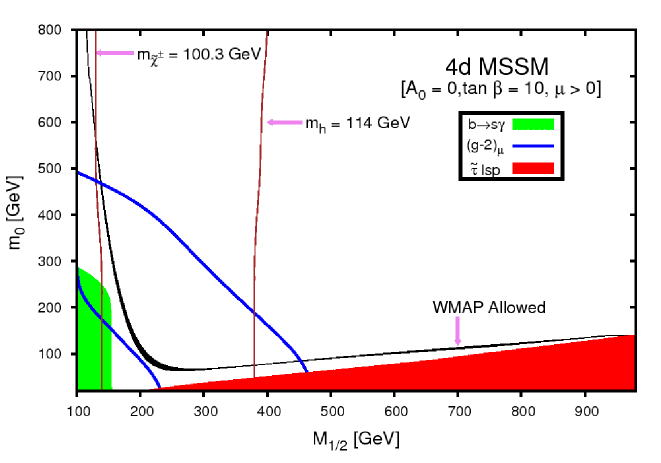
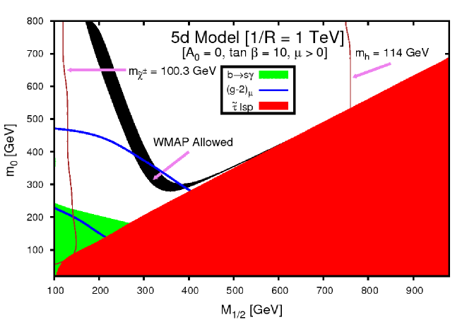
(a)                (b)

Figure 4.6: The $m_{0}-M_{1/2}$ parameter space for $\mu>0$ . We keep $tan\beta=10$ for all the plots. The region ruled out by $B(b\rightarrow s\gamma)$ is shaded in light green (lightest shade) ,the $\tilde{\tau}$ LSP region is shaded in red (darker shade) and the region favored by $(g-2)_{\mu}$ is the region between the two blue (darkest shade) lines. The WMAP allowed region where $.087<\Omega_{DM}h^{2}<.138$ is shaded in black. We also show the contours for $m_{h}=114GeV$ and $m_{\tilde{\chi}^{\pm}}=103.3GeV$, the region to the left of these lines are ruled out by the lep exclusion limits. For the 5d models, the Higgs contour shown does not include the KK contribution.

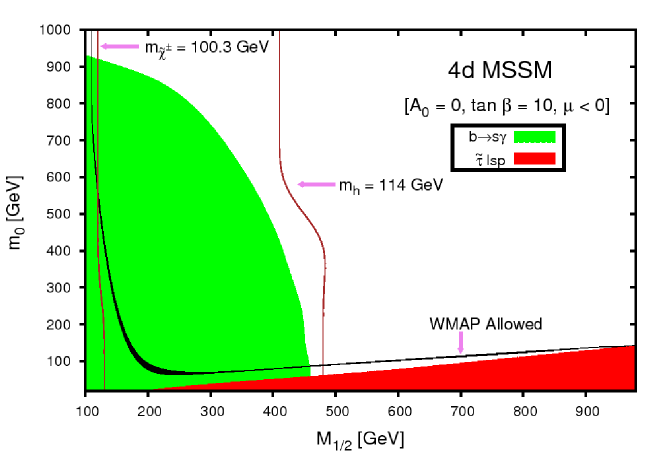
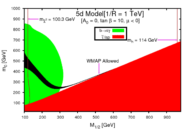
(a)                (b)

Figure 4.7: Same as Figure 4.6 for $\mu<0$. The entire region is now disfavored by the $(g-2)_{\mu}$.

Chapter 5 Summary and Conclusions

We have entered the LHC era with confidence in our belief in the existence of a theory beyond the standard model. We already have experimental evidences in its favour from the electro-weak sector, like the exixtance neutrino mass. Expectations are mounting that the LHC will discover some of these new physics, turning decades of speculation into experimental realities. Certainly it will pave the way for future research in this field.

New physics of different incarnations, especially supersymmetry and/or extra dimensions, are crying out for validation. And the LHC is expected to sit on judgement on them. At this crucial juncture in the development of particle physics, we consider it relevant to study the phenomenology of these scenarios that are testable at the collider experiments already underway (like the LHC) or is at the planning stage (like the ILC). In this thesis we have studied the formal and phenomenological aspects of supersymmetry, extra dimension and their interface.

In the second chapter of this thesis we discuss the impact of warped extra dimension on the processes $gg\to h$ and $h\to\gamma\gamma$, that are of paramount importance in the context of Higgs search at the LHC. These processes are loop driven and hence could be sensitive to the presence of any new colored fermion states having a large coupling with the Higgs. We confine Higgs field to the TeV brane and the hierarchy of fermion masses is addressed by localizing them at different positions in the bulk. We show that the Yukawa coupling of the Higgs with the fermion Kaluza-Klein (KK) states can be order one irrespective of their zero mode masses. We observe that the $gg\to h$ and $h\to\gamma\gamma$ rates are substantially altered if the KK states lie within the reach of LHC. We found that inspite of completely different reasons, the numerical impact of the RS model is comparable to the UED scenario.

In chapter three we compute radiative correction to the lightest neutral Higgs mass ($m_{h}$) induced by the Kaluza-Klein (KK) towers of fermions and sfermions in a minimal supersymmetric scenario embeded in a 5-dimensional warped space. The Higgs is again confined to the TeV brane, providing a handle to address the $\mu$ problem. The KK spectrum of matter supermultiplets is tied to the explanation of the fermion mass hierarchy . We demonstrate that for a reasonable choice of extra-dimensional parameters, the KK-induced radiative correction can enhance the upper limit on $m_{h}$ by as much as 100 GeV beyond the 4d limit of 135 GeV. Here the impact is still significant but more modest as compared to UED scenario, considering the more restrictive constraints on the RS scenario comming from precision electroweak observables.

In the fourth chapter of this thesis we studied the running of the soft parameters and the couplings of the minimal supersymmetric standard model embedded in a flat extra dimension compactified on an $S_{1}/\mathbb{Z}_{2}$ orbifold. In order to keep the theory perturbative at all scales we restricted the first two generations of fermions to the 3-branes, allowing all other fields to access the extra dimension. We computed the contributions of the Kaluza-Klein (KK) towers to the various one-loop $\beta$ functions. We demonstrated that radiative electroweak symmetry breaking can be achieved in this scenario. We also put constraints on the $m_{0}-M_{{1}/{2}}$ plane of the theory from various theoretical considerations and experimental observations. We have incorporated constraints coming from direct LEP search for supersymmetric particles, Higgs mass limit, anomalous magnetic moment of the muon $(g-2)_{\mu}$, the $\rho$ parameter, branching ratio of $b\rightarrow s\gamma$ and WMAP probe for relative dark matter abundance. Our plots are the first 5d versions of the often displayed 4d $m_{0}$–$M_{1/2}$ plots. We also study the reasons behind the differences between the 4d and 5d plots which arises mainly from the effect of the supersymmetric ($N=1$ & $N=2$) non-renormalization theorems.

Bibliography

- [1] Books on quantum field theory: e.g M. Peskin and D. Schroeder, An Introduction to Quantum Field Theory” (Perseus Books, Cambridge, 1995), T-P Cheng and L-F Li,Gauge theory of elementary particle physics” (Clarendon Press, Oxford, 1984)
- [2] S. L. Glashow, Nucl. Phys. 22 (1961) 579; A. Salam and J. C. Ward, Phys. Lett. 13 (1964) 168, A. Salam, Elementary Particle Theory, Proceedings Of The Nobel Symposium Held 1968 At Lerum, Sweden*, ed. N. Svartholm (Almquist and Wiksell, Stockholm, 1968) 367-377; S. Weinberg, Phys. Rev. Lett. 19 (1967) 1264.
- [3] D. J. Gross, Proc. Nat. Acad. Sci. 102 (2005) 9099-9108; S. Bethke, Prog. Part. Nucl. Phys. 58 (2007) 351-386 [hep-ex/0606035]; C. Amsler, A. Masoni, “The (1405), (1475), (1420), and (1510),”
- [4] D. J. Gross, F. Wilczek, Phys. Rev. Lett. 30 (1973) 1343-1346; H. D. Politzer, Phys. Rev. Lett. 30 (1973) 1346-1349.
- [5] H. Fritzsch, M. Gell-Mann, H. Leutwyler, Phys. Lett. B47 (1973) 365-368.
- [6] S. L. Glashow, J. Iliopoulos, L. Maiani, Phys. Rev. D2 (1970) 1285-1292.
- [7] N. Cabibbo, Phys. Rev. Lett. 10 (1963) 531-533.
- [8] M. Kobayashi, T. Maskawa, Prog. Theor. Phys. 49 (1973) 652-657.
- [9] R. Aleksan, B. Kayser, D. London, Phys. Rev. Lett. 73 (1994) 18-20 [hep-ph/9403341]; I. I. Y. Bigi, A. I. Sanda, [hep-ph/9909479].
- [10] C. Jarlskog, Phys. Rev. Lett. 55 (1985) 1039; C. Jarlskog, Z. Phys. C29 (1985) 491; C. Jarlskog and R. Stora, Phys. Lett. B208 (1988) 268.
- [11] C. Bouchiat, J. Iliopoulos, P. Meyer, Phys. Lett. B38 (1972) 519-523.
- [12] F. Englert, R. Brout, Phys. Rev. Lett. 13 (1964) 321-322; P. W. Higgs, Phys. Lett. 12 (1964) 132-133; P. W. Higgs, Phys. Rev. Lett. 13 (1964) 508-509; G. S. Guralnik, C. R. Hagen, T. W. B. Kibble, Phys. Rev. Lett. 13 (1964) 585-587.
- [13] V. L. Ginzburg, L. D. Landau, Zh. Eksp. Teor. Fiz. 20 (1950) 1064-1082.
- [14] T. W. B. Kibble, Phys. Rev. 155 (1967) 1554-1561.
- [15] Y. Nambu, Phys. Rev. Lett. 4 (1960) 380-382; Y. Nambu, G. Jona-Lasinio, Phys. Rev. 122 (1961) 345-358; J. Goldstone, Nuovo Cim. 19 (1961) 154-164; J. Goldstone, A. Salam, S. Weinberg, Phys. Rev. 127 (1962) 965-970.
- [16] G. Arnison et al. [ UA1 Collaboration ], Phys. Lett. B166 (1986) 484-490.
- [17] R. Ansari et al. [ UA2 Collaboration ], Phys. Lett. B186 (1987) 440-451.
- [18] C. Amsler et al., Phys. Lett. B667, p. 1 (2008).
- [19] T. D. Lee, C. S. Wu, Ann. Rev. Nucl. Part. Sci. 15 (1965) 381-476.
- [20] LEP Electroweak Working Group lepewwg.web.cern.ch.
- [21] H. Flacher, M. Goebel, J. Haller, A. Hocker, K. Monig, J. Stelzer, Eur. Phys. J. C60 (2009) 543-583 [arXiv:0811.0009 [hep-ph]].
- [22] C. Amsler et al. [ Particle Data Group Collaboration ], Phys. Lett. B667 (2008) 1-1340.
- [23] A. Cecucci, Z. Ligeti, and Y. Sakai, “The CKM quark-mixing matrix,” in [22].
- [24] J. Charles et al. [ CKMfitter Group Collaboration ], Eur. Phys. J. C41 (2005) 1-131 [hep-ph/0406184].
- [25] G. Bhattacharyya, Rept. Prog. Phys. 74 (2011) 026201 [arXiv:0910.5095 [hep-ph]].
- [26] M. E. Peskin and T. Takeuchi, Phys. Rev. Lett. 65 (1990) 964; W. J. Marciano and J. L. Rosner, Phys. Rev. Lett. 65 (1990) 2963 [Erratum-ibid. 68 (1992) 898]; D. C. Kennedy and P. Langacker, Phys. Rev. Lett. 65 (1990) 2967 [Erratum-ibid. 66 (1991) 395]; G. Altarelli and R. Barbieri, Phys. Lett. B 253 (1991) 161; G. Bhattacharyya, S. Banerjee and P. Roy, Phys. Rev. D 45 (1992) 729 [Erratum-ibid. D 46 (1992) 3215].
- [27] R. Barbieri, A. Pomarol, R. Rattazzi and A. Strumia, Nucl. Phys. B 703 (2004) 127 [arXiv:hep-ph/0405040].
- [28] For a more detailed discussion, see P. Langacker, [arXiv:hep-ph/0304186].
- [29] P. Kielanowski and S. R. Juarez W., Phys. Rev. D 72 (2005) 096003 [arXiv:hep-ph/0310122].
- [30] R. M. Carey et al., “The New (g-2) Experiment: A proposal to measure the muon anomalous magnetic moment to +-0.14 ppm precision,”, FERMILAB-PROPOSAL-0989
- [31] A. J. Buras, [arXiv:0910.1032 [hep-ph]].
- [32] D. Clowe, M. Bradac, A. H. Gonzalez, M. Markevitch, S. W. Randall, C. Jones, D. Zaritsky, Astrophys. J. 648 (2006) L109-L113 [astro-ph/0608407].
- [33] E. Komatsu et al. [WMAP Collaboration], Astrophys. J. Suppl. 180 (2009) 330 [arXiv:0803.0547 [astro-ph]].
- [34] A. D. Sakharov, Pisma Zh. Eksp. Teor. Fiz. 5 (1967) 32-35.
- [35] M. B. Green, J. H. Schwarz, E. Witten, Cambridge, Uk: Univ. Pr. ( 1987) 469 P. ( Cambridge Monographs On Mathematical Physics); M. B. Green, J. H. Schwarz, E. Witten, Cambridge, Uk: Univ. Pr. ( 1987) 596 P. ( Cambridge Monographs On Mathematical Physics).
- [36] J. Polchinski, Cambridge, UK: Univ. Pr. (1998) 402 p; J. Polchinski, Cambridge, UK: Univ. Pr. (1998) 531 p.
- [37] K. Becker, M. Becker, J. H. Schwarz, Cambridge, UK: Cambridge Univ. Pr. (2007) 739 p.
- [38] H. Georgi, S. L. Glashow, Phys. Rev. Lett. 32 (1974) 438-441.
- [39] P. Langacker, Phys. Rept. 72 (1981) 185.
- [40] G. G. Ross, Reading, Usa: Benjamin/cummings ( 1984) 497 P. ( Frontiers In Physics, 60).
- [41] J. L. Hewett, T. G. Rizzo, Phys. Rept. 183 (1989) 193.
- [42] S. Raby, Eur. Phys. J. C59 (2009) 223-247 [arXiv:0807.4921 [hep-ph]].
- [43] J. Preskill, Ann. Rev. Nucl. Part. Sci. 34 (1984) 461-530.
- [44] See, for example, M. R. Douglas, [arXiv:hep-th/0405279];
- [45] L. Susskind, In *Carr, Bernard (ed.): Universe or multiverse?* 247-266 [arXiv:hep-th/0302219].
- [46] For a review, see R. D. Peccei, Adv. Ser. Direct. High Energy Phys. 3 (1989) 503-551.
- [47] G. Bhattacharyya, Pramana 72 (2009) 37-54 [arXiv:0807.3883 [hep-ph]].
- [48] C. T. Hill, E. H. Simmons, Phys. Rept. 381 (2003) 235-402 [arXiv:hep-ph/0203079].
- [49] N. Arkani-Hamed, A. G. Cohen, E. Katz, A. E. Nelson, JHEP 0207 (2002) 034 [arXiv:hep-ph/0206021].
- [50] M. Perelstein, Prog. Part. Nucl. Phys. 58 (2007) 247-291 [arXiv:hep-ph/0512128].
- [51] Z. Chacko, H. -S. Goh, R. Harnik, Phys. Rev. Lett. 96 (2006) 231802 [arXiv:hep-ph/0506256].
- [52] C. Csaki, C. Grojean, L. Pilo, J. Terning, Phys. Rev. Lett. 92 (2004) 101802 [arXiv:hep-ph/0308038].
- [53] For reviews see, G. Bhattacharyya, Nucl. Phys. Proc. Suppl. 52A (1997) 83 [arXiv:hep-ph/9608415]; G. Bhattacharyya, [arXiv:hep-ph/9709395]; H. K. Dreiner, [arXiv:hep-ph/9707435]; M. Chemtob, Prog. Part. Nucl. Phys. 54 (2005) 71 [arXiv:hep-ph/0406029]; R. Barbier et al., Phys. Rept. 420 (2005) 1 [arXiv:hep-ph/0406039].
- [54] S. P. Martin, [arXiv:hep-ph/9709356], I. J. R. Aitchison, [arXiv:hep-ph/0505105].
- [55] N. Arkani-Hamed, S. Dimopoulos and G. R. Dvali, Phys. Lett. B 429 (1998) 263 [arXiv:hep-ph/9803315]; I. Antoniadis, N. Arkani-Hamed, S. Dimopoulos and G. R. Dvali, Phys. Lett. B 436 (1998) 257 [arXiv:hep-ph/9804398]; N. Arkani-Hamed, S. Dimopoulos and G. R. Dvali, Phys. Rev. D 59 (1999) 086004 [arXiv:hep-ph/9807344].
- [56] L. Randall and R. Sundrum, Phys. Rev. Lett. 83 (1999) 3370 [arXiv:hep-ph/9905221].
- [57] See e.g., H. E. Haber and G. L. Kane, Phys. Rept. 117 (1985) 75; H. P. Nilles, Phys. Rept. 110 (1984)1; M. Drees, R. Godbole and P. Roy, “Theory and phenomenology of sparticles: An account of four-dimensional N=1 supersymmetry in high energy physics,” (World Scientific, Singapore, 2004); H. Baer and X. Tata, “Weak scale supersymmetry: From superfields to scattering events,” (UK: Univ. Pr., Cambridge, 2006); A. Djouadi, [arXiv:hep-ph/0503173].
- [58] For a recent reveiw, see, J. Ellis, G. Ridolfi and F. Zwirner, “Higgs boson properties in the standard model and its supersymmetric extensions,” To be published in ”Search of the Higgs Particle”, Comptes Rendus de l’Academie des Sciences, France, [arXiv:hep-ph/0702114].
- [59] J. R. Ellis, S. Kelley, D. V. Nanopoulos, Phys. Lett. B260 (1991) 131-137; U. Amaldi, W. de Boer, H. Furstenau, Phys. Lett. B260 (1991) 447-455.
- [60] S. Coleman and J. Mandula, Phys. Rev. 159 (1967) 1251; R. Haag, J. T. Lopuszanski, M. Sohnius, Nucl. Phys. B88 (1975) 257.
- [61] G. L. Kane, C. F. Kolda, J. D. Wells, Phys. Rev. Lett. 70 (1993) 2686-2689 [arXiv:hep-ph/9210242]; J. R. Espinosa, M. Quiros, Phys. Lett. B302 (1993) 51-58 [arXiv:hep-ph/9212305].
- [62] H. Baer, C. -h. Chen, F. Paige, X. Tata, Phys. Rev. D52 (1995) 2746-2759 [arXiv:hep-ph/9503271]; H. Baer, C. -h. Chen, F. Paige, X. Tata, Phys. Rev. D53 (1996) 6241-6264 [arXiv:hep-ph/9512383]; H. Baer, C. -h. Chen, M. Drees, F. Paige, X. Tata, Phys. Rev. D59 (1999) 055014 [arXiv:hep-ph/9809223].
- [63] F. del Aguila, L. Ametller, Phys. Lett. B261 (1991) 326-333; H. Baer, C. -h. Chen, F. Paige, X. Tata, Phys. Rev. D49 (1994) 3283-3290 [arXiv:hep-ph/9311248].
- [64] P. R. Harrison, C. H. Llewellyn Smith, Nucl. Phys. B213 (1983) 223 [Erratum-ibid. B 223, (1983)542]; G. L. Kane, J. P. Leveille, Phys. Lett. B112 (1982) 227; S. Dawson, E. Eichten, C. Quigg, Phys. Rev. D31 (1985) 1581; H. Baer, X. Tata, Phys. Lett. B160 (1985) 159. Significant next-to-leading order corrections have been computed in W. Beenakker, R. Hopker, M. Spira, P. M. Zerwas, Phys. Rev. Lett. 74 (1995) 2905-2908 [arXiv:hep-ph/9412272]; W. Beenakker, R. Hopker, M. Spira, P. M. Zerwas, Z. Phys. C69 (1995) 163-166 [arXiv:hep-ph/9505416]; W. Beenakker, R. Hopker, M. Spira, P. M. Zerwas, Nucl. Phys. B492 (1997) 51-103 [arXiv:hep-ph/9610490]; W. Beenakker, M. Klasen, M. Kramer, T. Plehn, M. Spira, P. M. Zerwas, Phys. Rev. Lett. 83 (1999) 3780-3783 [arXiv:hep-ph/9906298].
- [65] Theres been a lot of recent work on this subject; see, for example, G. Cacciapaglia, C. Csaki, C. Grojean, J. Terning, Phys. Rev. D71 (2005) 035015 [arXiv:hep-ph/0409126]; G. Cacciapaglia, C. Csaki, C. Grojean, J. Terning, Phys. Rev. D70 (2004) 075014 [arXiv:hep-ph/0401160]; C. Csaki, C. Grojean, J. Hubisz, Y. Shirman, J. Terning, Phys. Rev. D70 (2004) 015012 [arXiv:hep-ph/0310355]; C. Csaki, C. Grojean, L. Pilo, J. Terning, Phys. Rev. Lett. 92 (2004) 101802 [arXiv:hep-ph/0308038]; C. Csaki, C. Grojean, H. Murayama, L. Pilo, J. Terning, Phys. Rev. D69 (2004) 055006 [arXiv:hep-ph/0305237]; Y. Nomura, JHEP 0311 (2003) 050 [arXiv:hep-ph/0309189]; J. L. Hewett, B. Lillie, T. G. Rizzo, JHEP 0410 (2004) 014 [arXiv:hep-ph/0407059]; H. Davoudiasl, J. L. Hewett, B. Lillie, T. G. Rizzo, JHEP 0405 (2004) 015 [arXiv:hep-ph/0403300]; H. Davoudiasl, J. L. Hewett, B. Lillie, T. G. Rizzo, Phys. Rev. D70 (2004) 015006. [arXiv:hep-ph/0312193] and R. Barbieri, A. Pomarol, R. Rattazzi, Phys. Lett. B591 (2004) 141-149 [arXiv:hep-ph/0310285].
- [66] Some sample analyses can be found in N. Arkani-Hamed, S. Dimopoulos, G. R. Dvali, J. March-Russell, Phys. Rev. D65 (2002) 024032 [arXiv:hep-ph/9811448]; N. Arkani-Hamed, Y. Grossman, M. Schmaltz, Phys. Rev. D61 (2000) 115004 [arXiv:hep-ph/9909411]; N. Arkani-Hamed, M. Schmaltz, Phys. Rev. D61 (2000) 033005 [arXiv:hep-ph/9903417]; B. Lillie, JHEP 0312 (2003) 030 [arXiv:hep-ph/0308091]; B. Lillie, J. L. Hewett, Phys. Rev. D68 (2003) 116002 [arXiv:hep-ph/0306193]; K. Agashe, G. Perez, A. Soni, Phys. Rev. D71 (2005) 016002 [arXiv:hep-ph/0408134].
- [67] K. R. Dienes, E. Dudas, T. Gherghetta, Nucl. Phys. B537 (1999) 47-108 [arXiv:hep-ph/9806292]; K. R. Dienes, E. Dudas, T. Gherghetta, Phys. Lett. B436 (1998) 55-65 [arXiv:hep-ph/9803466]; L. Randall, M. D. Schwartz, Phys. Rev. Lett. 88 (2002) 081801 [arXiv:hep-th/0108115]; L. Randall, M. D. Schwartz, JHEP 0111 (2001) 003 [arXiv:hep-th/0108114]; M. S. Carena, A. Delgado, E. Ponton, T. M. P. Tait, C. E. M. Wagner, Phys. Rev. D68 (2003) 035010 [arXiv:hep-ph/0305188].
- [68] T. Appelquist, H. -C. Cheng, B. A. Dobrescu, Phys. Rev. D64 (2001) 035002 [arXiv:hep-ph/0012100]; H. -C. Cheng, K. T. Matchev, M. Schmaltz, Phys. Rev. D66 (2002) 056006 [arXiv:hep-ph/0205314]; H. -C. Cheng, K. T. Matchev, M. Schmaltz, Phys. Rev. D66 (2002) 036005 [arXiv:hep-ph/0204342]; G. Servant, T. M. P. Tait, Nucl. Phys. B650 (2003) 391-419 [arXiv:hep-ph/0206071].
- [69] For an introduction, see P. Binetruy, C. Deffayet, D. Langlois, Nucl. Phys. B565 (2000) 269-287 [arXiv:hep-th/9905012].
- [70] S. Dimopoulos, G. L. Landsberg, Phys. Rev. Lett. 87 (2001) 161602 [arXiv:hep-ph/0106295]; S. B. Giddings, S. D. Thomas, Phys. Rev. D65 (2002) 056010 [arXiv:hep-ph/0106219]; For a recent update, see S. B. Giddings, V. S. Rychkov, Phys. Rev. D70 (2004) 104026 [arXiv:hep-th/0409131].
- [71] E. Recami, Riv. Nuovo Cim. 9N6 (1986) 1-178.
- [72] G. R. Dvali, G. Gabadadze, G. Senjanovic, In *Shifman, M.A. (ed.): The many faces of the superworld* 525-532 [arXiv:hep-ph/9910207].
- [73] G. Bhattacharyya and T. S. Ray, Phys. Lett. B 675 (2009) 222 [arXiv:0902.1893 [hep-ph]].
- [74] V. A. Rubakov, M. E. Shaposhnikov, Phys. Lett. B125 (1983) 139; V. A. Rubakov, M. E. Shaposhnikov, Phys. Lett. B125 (1983) 136-138.
- [75] C. Csaki, [arXiv:hep-ph/0404096].
- [76] N. Arkani-Hamed, S. Dimopoulos, N. Kaloper, R. Sundrum, Phys. Lett. B480 (2000) 193-199 [arXiv:hep-th/0001197]; S. Kachru, M. B. Schulz, E. Silverstein, Phys. Rev. D62 (2000) 045021 [arXiv:hep-th/0001206]; S. Forste, Z. Lalak, S. Lavignac, H. P. Nilles, Phys. Lett. B481 (2000) 360-364 [arXiv:hep-th/0002164]; C. Csaki, J. Erlich, C. Grojean, T. J. Hollowood, Nucl. Phys. B584 (2000) 359-386 [arXiv:hep-th/0004133]; C. Csaki, J. Erlich, C. Grojean, Nucl. Phys. B604 (2001) 312-342 [arXiv:hep-th/0012143].
- [77] T. Gherghetta and A. Pomarol, Nucl. Phys. B 586 (2000) 141 [arXiv:hep-ph/0003129].
- [78] Y. Grossman and M. Neubert, Phys. Lett. B 474 (2000) 361 [arXiv:hep-ph/9912408].
- [79] A. Pomarol, Phys. Lett. B 486 (2000) 153 [arXiv:hep-ph/9911294].
- [80] W. D. Goldberger, M. B. Wise, Phys. Rev. Lett. 83 (1999) 4922-4925 [arXiv:hep-ph/9907447].
- [81] C. Csaki, M. Graesser, L. Randall, J. Terning, Phys. Rev. D62 (2000) 045015 [arXiv:hep-ph/9911406].
- [82] W. D. Goldberger, M. B. Wise, Phys. Lett. B475 (2000) 275-279 [arXiv:hep-ph/9911457].
- [83] C. Charmousis, R. Gregory, V. A. Rubakov, Phys. Rev. D62 (2000) 067505 [arXiv:hep-th/9912160].
- [84] C. Csaki, J. Erlich, T. J. Hollowood, Y. Shirman, Nucl. Phys. B581 (2000) 309-338 [arXiv:hep-th/0001033].
- [85] O. DeWolfe, D. Z. Freedman, S. S. Gubser, A. Karch, Phys. Rev. D62 (2000) 046008 [arXiv:hep-th/9909134].
- [86] C. Csaki, J. Erlich, C. Grojean, T. J. Hollowood, Nucl. Phys. B584 (2000) 359-386 [arXiv:hep-th/0004133].
- [87] C. Csaki, M. L. Graesser, G. D. Kribs, Phys. Rev. D63 (2001) 065002 [arXiv:hep-th/0008151].
- [88] P. Kanti, I. I. Kogan, K. A. Olive, M. Pospelov, Phys. Lett. B468 (1999) 31-39 [arXiv:hep-ph/9909481]; P. Kanti, I. I. Kogan, K. A. Olive, M. Pospelov, Phys. Rev. D61 (2000) 106004 [arXiv:hep-ph/9912266].
- [89] T. Tanaka, X. Montes, Nucl. Phys. B582 (2000) 259-276 [arXiv:hep-th/0001092].
- [90] K. Agashe, A. Falkowski, I. Low and G. Servant, JHEP 0804 (2008) 027
- [91] W. D. Goldberger and M. B. Wise, Phys. Rev. Lett. 83 (1999) 4922 [arXiv:hep-ph/9907447]; W. D. Goldberger and M. B. Wise, Phys. Lett. B 475 (2000) 275 [arXiv:hep-ph/9911457]; H. Davoudiasl, J. L. Hewett and T. G. Rizzo, Phys. Lett. B 473 (2000) 43 [arXiv:hep-ph/9911262]; A. Pomarol, Phys. Lett. B 486 (2000) 153 [arXiv:hep-ph/9911294]; S. Chang, J. Hisano, H. Nakano, N. Okada and M. Yamaguchi, Phys. Rev. D 62 (2000) 084025. [arXiv:hep-ph/9912498]; A. Pomarol, Phys. Lett. B 486 (2000) 153 [arXiv:hep-ph/9911294].
- [92] S. J. Huber and Q. Shafi, Phys. Lett. B 498 (2001) 256 [arXiv:hep-ph/0010195].
- [93] K. Agashe, S. Gopalakrishna, T. Han, G. Y. Huang and A. Soni, [arXiv:0810.1497 [hep-ph]]; K. Agashe et al., Phys. Rev. D 76 (2007) 115015 [arXiv:0709.0007 [hep-ph]]; K. Agashe, A. Belyaev, T. Krupovnickas, G. Perez and J. Virzi, Phys. Rev. D 77 (2008) 015003 [arXiv:hep-ph/0612015]; K. Agashe, G. Perez and A. Soni, Phys. Rev. D 75 (2007) 015002. [arXiv:hep-ph/0606293]; F. Ledroit, G. Moreau and J. Morel, JHEP 0709 (2007) 071 [arXiv:hep-ph/0703262]; A. Djouadi, G. Moreau and R. K. Singh, Nucl. Phys. B 797 (2008) 1 [arXiv:0706.4191 [hep-ph]].
- [94] F. J. Petriello, JHEP 0205 (2002) 003 [arXiv:hep-ph/0204067].
- [95] S. K. Rai, Int. J. Mod. Phys. A 23 (2008) 823 [arXiv:hep-ph/0510339].
- [96] J. L. Hewett, F. J. Petriello and T. G. Rizzo, JHEP 0209 (2002) 030 [arXiv:hep-ph/0203091]; C. Csaki, J. Erlich and J. Terning, Phys. Rev. D 66 (2002) 064021 [arXiv:hep-ph/0203034].
- [97] K. Agashe, A. Delgado, M. J. May and R. Sundrum, JHEP 0308 (2003) 050 [arXiv:hep-ph/0308036].
- [98] C. Bouchart and G. Moreau, Nucl. Phys. B 810 (2009) 66 [arXiv:0807.4461 [hep-ph]].
- [99] M. S. Carena, E. Ponton, J. Santiago and C. E. M. Wagner, Phys. Rev. D 76 (2007) 035006 [arXiv:hep-ph/0701055]; M. S. Carena, E. Ponton, J. Santiago and C. E. M. Wagner, Nucl. Phys. B 759 (2006) 202 [arXiv:hep-ph/0607106].
- [100] A. Djouadi and G. Moreau, Phys. Lett. B 660 (2008) 67 [arXiv:0707.3800 [hep-ph]].
- [101] G. Cacciapaglia, A. Deandrea and J. Llodra-Perez, arXiv:0901.0927 [hep-ph].
- [102] A. Falkowski, Phys. Rev. D 77 (2008) 055018 [arXiv:0711.0828 [hep-ph]]; N. Maru and N. Okada, Phys. Rev. D 77 (2008) 055010 [arXiv:0711.2589 [hep-ph]].
- [103] K. R. Dienes, E. Dudas and T. Gherghetta, Nucl. Phys. B 567 (2000) 111 [arXiv:hep-ph/9908530].
- [104] T. Gherghetta and A. Pomarol, Nucl. Phys. B 602 (2001) 3 [arXiv:hep-ph/0012378].
- [105] M. Drees, Int. J. Mod. Phys. A 4 (1989) 3635; U. Ellwanger and C. Hugonie, Phys. Lett. B 623 (2005) 93.
- [106] Y. Zhang, H. An, X. d. Ji and R. N. Mohapatra, [arXiv:0804.0268 [hep-ph]].
- [107] G. Bhattacharyya, S. K. Majee and T. S. Ray, Phys. Rev. D 78 (2008) 071701 [arXiv:0806.3672 [hep-ph]].
- [108] N. Arkani-Hamed, T. Gregoire and J. G. Wacker, JHEP 0203 (2002) 055 [arXiv:hep-th/0101233].
- [109] A. Pomarol, [hep-ph/9911294].
- [110] J. R. Ellis, G. Ridolfi and F. Zwirner, Phys. Lett. B 257 (1991) 83 and Phys. Lett. B 262 (1991) 477; Y. Okada, M. Yamaguchi and T. Yanagida, Prog. Theor. Phys. 85 (1991) 1; H. E. Haber and R. Hempfling, Phys. Rev. Lett. 66 (1991) 1815; A. Brignole, Phys. Lett. B 281 (1992) 284; M. S. Berger, Phys. Rev. D41 (1990) 225; J. F. Gunion and A. Turski, Phys. Rev. D39 (1989) 2701.
- [111] M. Carena, J. R. Espinosa, M. Quiros and C. E. M. Wagner, Phys. Lett. B 355 (1995) 209 [arXiv:hep-ph/9504316]; M. Carena, M. Quiros and C. E. M. Wagner, Nucl. Phys. B 461 (1996) 407 [arXiv:hep-ph/9508343]; H. E. Haber, R. Hempfling and A. H. Hoang, Z. Phys. C 75 (1997) 539 [arXiv:hep-ph/9609331]; S. Heinemeyer, W. Hollik and G. Weiglein, Eur. Phys. J. C 9 (1999) 343 [arXiv:hep-ph/9812472].
- [112] G. Bhattacharyya, S. K. Majee and A. Raychaudhuri, Nucl. Phys. B 793 (2008) 114 [arXiv:0705.3103 [hep-ph]]. See also, N. Uekusa, [arXiv:0806.3229 [hep-ph]].
- [113] [arXiv:hep-ex/0306033]; [arXiv:hep-ex/0602042]; J. Alcaraz et al. [LEP Collaboration], “A combination of preliminary electroweak measurements and constraints on the standard model,” [arXiv:hep-ex/0612034].
- [114] I. Antoniadis, Phys. Lett. B 246 (1990) 377.
- [115] T. Appelquist, H. C. Cheng and B. A. Dobrescu, Phys. Rev. D 64 (2001) 035002 [arXiv:hep-ph/0012100].
- [116] P. Nath and M. Yamaguchi, Phys. Rev. D 60 (1999) 116006 [arXiv:hep-ph/9903298].
- [117] D. Chakraverty, K. Huitu and A. Kundu, Phys. Lett. B 558 (2003) 173 [arXiv:hep-ph/0212047].
- [118] K. Agashe, N. G. Deshpande and G. H. Wu, Phys. Lett. B 514 (2001) 309 [arXiv:hep-ph/0105084].
- [119] A. J. Buras, M. Spranger and A. Weiler, Nucl. Phys. B 660 (2003) 225 [arXiv:hep-ph/0212143]; A. J. Buras, A. Poschenrieder, M. Spranger and A. Weiler, Nucl. Phys. B 678 (2004) 455 [arXiv:hep-ph/0306158].
- [120] J. F. Oliver, J. Papavassiliou and A. Santamaria, Phys. Rev. D 67 (2003) 056002 [arXiv:hep-ph/0212391].
- [121] T. Appelquist and H. U. Yee, Phys. Rev. D 67 (2003) 055002 [arXiv:hep-ph/0211023].
- [122] I. Antoniadis, K. Benakli and M. Quiros, Phys. Lett. B 331 (1994) 313 [arXiv:hep-ph/9403290]; T. Rizzo, Phys. Rev. D 64 (2001) 095010 [arXiv:hep-ph/0106336]; C. Macesanu, C.D. McMullen and S. Nandi, Phys. Rev. D 66 (2002) 015009 [arXiv:hep-ph/0201300]; Phys. Lett. B 546 (2002) 253 [arXiv:hep-ph/0207269]; H.-C. Cheng, Int. J. Mod. Phys. A 18 (2003) 2779 [arXiv:hep-ph/0206035]; A. Muck, A. Pilaftsis and R. Rückl, Nucl. Phys. B 687 (2004) 55 [arXiv:hep-ph/0312186].
- [123] U. Haisch and A. Weiler, Phys. Rev. D 76 (2007) 034014 [arXiv:hep-ph/0703064].
- [124] G. Bhattacharyya, A. Datta, S. K. Majee and A. Raychaudhuri, Nucl. Phys. B 821 (2009) 48 [arXiv:0904.0937 [hep-ph]]; D. Choudhury, A. Datta and K. Ghosh, arXiv:0911.4064 [hep-ph].
- [125] E. Accomando, I. Antoniadis and K. Benakli, Nucl. Phys. B 579 (2000) 3 [arXiv:hep-ph/9912287].
- [126] P. Nath, Y. Yamada and M. Yamaguchi, Phys. Lett. B 466 (1999) 100 [arXiv:hep-ph/9905415]. M. Masip and A. Pomarol, Phys. Rev. D 60 (1999) 096005 [arXiv:hep-ph/9902467]. T. G. Rizzo and J. D. Wells, Phys. Rev. D 61 (2000) 016007 [arXiv:hep-ph/9906234]; A. Strumia, Phys. Lett. B 466 (1999) 107 [arXiv:hep-ph/9906266]; C. D. Carone, Phys. Rev. D 61 (2000) 015008 [arXiv:hep-ph/9907362].
- [127] G. Servant and T. M. P. Tait, Nucl. Phys. B 650 (2003) 391 [arXiv:hep-ph/0206071].
- [128] N. Arkani-Hamed, H. C. Cheng, B. A. Dobrescu and L. J. Hall, Phys. Rev. D 62 (2000) 096006 [arXiv:hep-ph/0006238].
- [129] N. Arkani-Hamed and M. Schmaltz, Phys. Rev. D 61 (2000) 033005 [arXiv:hep-ph/9903417].
- [130] A. Delgado, A. Pomarol and M. Quiros, JHEP 0001 (2000) 030 [arXiv:hep-ph/9911252].
- [131] K. R. Dienes, E. Dudas and T. Gherghetta, Nucl. Phys. B 537 (1999) 47 [arXiv:hep-ph/9806292].
- [132] K. R. Dienes, E. Dudas and T. Gherghetta, Phys. Lett. B 436 (1998) 55 [arXiv:hep-ph/9803466].
- [133] G. Bhattacharyya, A. Datta, S. K. Majee and A. Raychaudhuri, Nucl. Phys. B 760 (2007) 117 [arXiv:hep-ph/0608208].
- [134] A. Hebecker and A. Westphal, Annals Phys. 305 (2003) 119 [arXiv:hep-ph/0212175].
- [135] G. Bhattacharyya, S. Goswami and A. Raychaudhuri, Phys. Rev. D 66 (2002) 033008 [arXiv:hep-ph/0202147].
- [136] A. Deandrea, J. Welzel, P. Hosteins and M. Oertel, Phys. Rev. D 75 (2007) 113005 [arXiv:hep-ph/0611172].
- [137] B. S. Acharya, K. Bobkov, G. L. Kane, P. Kumar and J. Shao, Phys. Rev. D 76 (2007) 126010 [arXiv:hep-th/0701034]; B. S. Acharya, K. Bobkov, G. Kane, P. Kumar and D. Vaman, Phys. Rev. Lett. 97 (2006) 191601 [arXiv:hep-th/0606262]; J. J. Heckman, C. Vafa, H. Verlinde and M. Wijnholt, JHEP 0806 (2008) 016 [arXiv:0711.0387 [hep-ph]]; I. Antoniadis and S. Dimopoulos, Nucl. Phys. B 715 (2005) 120 [arXiv:hep-th/0411032]; R. Blumenhagen, J. P. Conlon, S. Krippendorf, S. Moster and F. Quevedo, JHEP 0909 (2009) 007 [arXiv:0906.3297 [hep-th]]; T. Banks and M. Dine, Nucl. Phys. B 479 (1996) 173 [arXiv:hep-th/9605136].
- [138] I. Antoniadis, C. Munoz and M. Quiros, Nucl. Phys. B 397 (1993) 515 [arXiv:hep-ph/9211309]; K. Benakli, Phys. Lett. B 386 (1996) 106 [arXiv:hep-th/9509115]; I. Antoniadis, S. Dimopoulos and G. R. Dvali, Nucl. Phys. B 516 (1998) 70 [arXiv:hep-ph/9710204].
- [139] G. Bhattacharyya, T. S. Ray, JHEP 1005 (2010) 040 [arXiv:1003.1276 [hep-ph]].
- [140] R. Barbieri, S. Ferrara, L. Maiani, F. Palumbo and C. A. Savoy, Phys. Lett. B 115 (1982) 212.
- [141] J. Scherk and J. H. Schwarz, Nucl. Phys. B 153 (1979) 61; J. Scherk and J. H. Schwarz, Phys. Lett. B 82 (1979) 60.
- [142] A. Pomarol and M. Quiros, Phys. Lett. B 438 (1998) 255 [arXiv:hep-ph/9806263]; A. Delgado, A. Pomarol and M. Quiros, Phys. Rev. D 60 (1999) 095008 [arXiv:hep-ph/9812489]; I. Antoniadis, S. Dimopoulos, A. Pomarol and M. Quiros, Nucl. Phys. B 544 (1999) 503 [arXiv:hep-ph/9810410]; D. Diego, G. von Gersdorff and M. Quiros, Phys. Rev. D 74 (2006) 055004 [arXiv:hep-ph/0605024]; G. von Gersdorff, Mod. Phys. Lett. A 22 (2007) 385 [arXiv:hep-ph/0701256].
- [143] R. Barbieri, L. J. Hall and Y. Nomura, Phys. Rev. D 63 (2001) 105007 [arXiv:hep-ph/0011311].
- [144] E. A. Mirabelli and M. E. Peskin, Phys. Rev. D 58 (1998) 065002 [arXiv:hep-th/9712214].
- [145] Z. Chacko, M. A. Luty, A. E. Nelson and E. Ponton, JHEP 0001 (2000) 003 [arXiv:hep-ph/9911323].
- [146] N. Arkani-Hamed, L. J. Hall, Y. Nomura, D. Tucker-Smith and N. Weiner, Nucl. Phys. B 605 (2001) 81 [arXiv:hep-ph/0102090].
- [147] G. Belanger, F. Boudjema, A. Pukhov and A. Semenov, Comput. Phys. Commun. 149 (2002) 103 [arXiv:hep-ph/0112278]. G. Belanger, F. Boudjema, A. Pukhov and A. Semenov, Comput. Phys. Commun. 176 (2007) 367 [arXiv:hep-ph/0607059].
- [148] A. Djouadi, M. Drees and J. L. Kneur, JHEP 0603 (2006) 033 [arXiv:hep-ph/0602001].
- [149] E. Barberio et al. [Heavy Flavor Averaging Group], [arXiv:0808.1297 [hep-ex]].
- [150] D. E. Kaplan, G. D. Kribs and M. Schmaltz, Phys. Rev. D 62 (2000) 035010 [arXiv:hep-ph/9911293].