The lowest scattering state of one-dimensional Bose gas with attractive interactions

Abstract

We investigate the lowest scattering state of one-dimensional Bose gas with attractive interactions trapped in a hard wall trap. By solving the Bethe ansatz equation numerically we determine the full energy spectrum and the exact wave function for different attractive interaction parameters. The resultant density distribution, momentum distribution, reduced one body density matrix and two body correlation show that the decreased attractive interaction induces rich density profiles and specific correlation properties in the weakly attractive Bose gas.

I Introduction

With the rapid experimental progress the ultracold atomic gases have offered a popular platform to investigate the strongly correlated one dimensional many-body systems gorlitz ; esslinger ; Paredes ; Toshiya for their high controllability and tunability. One dimensional quantum gases can be realized with strong anisotropic magnetic trap or two dimensional optical lattice Stoeferle ; Paredes ; Toshiya ; HallerPRL and be described theoretically by an effective one dimensional (1D) model Olshanii ; Olshanii2 ; Petrov ; Dunjko . In addition the effective 1D interaction can be tuned from the strongly attractive to the strongly repulsive interacting regime via the magnetic Feshbach resonance or confinement induced resonance. Not only the strongly interacting Tonks-Girardeau (TG) gases TG but also two counter-intuitive examples, i.e., the repulsively bound atom pairs Winkler and the super Tonks-Girardeau (STG) gas-like phase of the attractive atomic gas Haller ; Astrakharchik ; Batchelor , have been realized by a sudden quench of interaction from the strong repulsion to the strong attraction or vice versa, both of which are hard to realize in the traditional condensed matter physics and have no analog in solid state systems. It has been displayed that they are stable excited states and the stability could be understood from the quench dynamics of the 1D integrable quantum gas STGChen . So far, the STG gas has attracted intensive theoretical studies from various aspects Kormos ; STGChen3 ; Muth ; GirardeauSTG ; STGChen2 .

The experimental realization of STG gases and repulsively bound atom pairs open the door to stable highly excited quantum many-body phases. This also offers us a method to search for exotic quantum phases in 1D many-body systems. It has been predicted that such stable excited states can be prepared in optical lattice via sudden quantum quench STGChen3 and the effective super Tonks-Girardeau gases can be realized via strongly attractive one-dimensional Fermi gases STGChen2 . Theoretically the strongly interacting Bose gases cannot be well described in the mean-field theory due to the large quantum fluctuation in 1D system and one has to resort to non-perturbation methods. Many methods such as Bethe ansatz Dunjko ; Fuchs ; Hao ; Guan , Bosonization method Cazalilla , exact diagonalization Deuretzbacher ; HaoEPJD , Bose-Fermi mapping method (BFM) Girardeau07 and multi-configuration Hartree theory Alon were used to investigate the 1D quantum gases. It was shown that with the increase in repulsion strength the ground state density distribution of 1D Bose gases continuously evolves from a Gaussian-like distribution to a multi-peak structure while the momentum distribution remains the single peak structure of bosonic atoms Hao ; HaoEPJD ; Deuretzbacher ; ferminization .

By a sudden quench of interaction from strong repulsion to strong attraction a TG gas shall transfer into a STG gas Haller ; STGChen ; GirardeauSTG . Because the quantum gas is very weakly coupled with the environment its energy dissipation is ignorable and this highly excited state shall be stable. By decreasing the attractive interaction of STG gas we can investigate the properties of the lowest scattering state for the Bose gas with the change of attractive interaction from strongly to weakly interacting regime. In this work, by numerically solving the Bethe ansatz equation we obtain exact wave function of the lowest scattering state of 1D Bose gas trapped in a hard wall potential in the above interacting regime. We will focus on the density distribution, reduced one body density matrix (ROBDM) and two body correlation in the full attractive interaction regime.

The present paper is organized as follows. Section II is devoted to the description of our model and Bethe Ansatz method. Section III will give the density profiles, ROBDM and two body correlation in the full attractive interacting regime. A summary is given in the last section.

II Model and method

We consider $N$ interacting Bose atoms of mass $m$ confined in a hard wall box of length $L$, which is described by the Hamiltonian

$$H=-\sum\limits_{i=1}^{N}\frac{\partial^{2}}{\partial x_{i}^{2}}+2c\sum\limits_{1\leq i\leq j\leq N}^{N}\delta(x_{i}-x_{j}).$$ (1)

Here the natural unit is used $\hbar=2m=1$ and $c=mg_{1D}/\hbar^{2}$ is an interaction constant dependent on the effective 1D interaction strength $g_{1D}$, which can be tuned continuously from the strong attraction to the strong repulsion by Feshbach resonance or confinement induced resonance. This model can be solved exactly by the Bethe ansatz method OPB . The many-particle wave function shall be formulated as the following general form

$$\Psi\left(x_{1},\cdots,x_{N}\right) = \sum_{Q}\theta\left(x_{q_{N}}-x_{q_{N-1}}\right)\cdots\theta\left(x_{q_{2}}-x_{q_{1}}\right)$$ (2)

$$\times\varphi_{Q}\left(x_{q_{1}},x_{q_{2}},\cdots,x_{q_{N}}\right)$$

with

$$\varphi_{Q}\left(x_{q_{1}},x_{q_{2}},\cdots,x_{q_{N}}\right)$$ (3)

$$= \sum_{P,r_{1},\ldots,r_{N}}\left[A\left(Q,rP\right)\exp\left(i\sum_{j}r_{p_{j}}k_{p_{j}}x_{q_{j}}\right)\right],$$

where $Q=(q_{1},q_{2},\cdots,q_{N})$ and $P=(p_{1},p_{2},\cdots,p_{N})$ are one of the permutations of $1,\cdots,N$, respectively, $A\left(Q,rP\right)$ is the abbreviation of the coefficient $A\left(q_{1},q_{2},\cdots,q_{N};r_{p_{1}}p_{1},r_{p_{2}}p_{2},\cdots,r_{p_{N}}p_{N}\right)$ to be determined self-consistently, and the summation $\sum_{P}$ ($\sum_{Q}$) is done for all of them. Here $r_{j}=\pm$ indicate that the particles move toward the right or the left, $\theta(x-y)$ is the step function and the parameters $\left\{k_{j}\right\}$ are known as quasi-momenta. In the following evaluation the length $L$ will be taken to be unity unless otherwise specified. For Bosons the wave function should follow the symmetry of exchange, so the present problem is simplified into the solution of

$$H\varphi_{1,...,N}\left(x_{1},\cdots,x_{N}\right)=E\varphi_{1,...,N}\left(x_{1},\cdots,x_{N}\right)$$ (4)

in the region of $0\leq x_{1}\leq x_{2}\leq\cdots\leq x_{N}\leq L$ with the open boundary condition

$$\varphi_{1,...,N}\left(\cdots,x_{j}=0,\cdots\right)=\varphi_{1,...,N}\left(\cdots,x_{j}=L,\cdots\right)=0.$$

For simplicity we shall ignore the subscript in $\varphi_{1,...,N}\left(x_{1},\cdots,x_{N}\right)$. The wave function in other region $Q$ can be obtained by the exchange symmetry of Bose wave function.

With some algebraic calculation, the wave function has the following explicit form

$$\varphi\left(x_{1},x_{2},\cdots,x_{N}\right)$$

$$= \sum_{P}A_{P}\in_{P}\exp\left[i\left(\sum_{l<j}^{N-1}\omega_{p_{j}p_{l}}\right)\right]\exp\left(ik_{p_{N}}L\right)\sin\left(k_{p_{1}}x_{1}\right)$$

$$\times\prod_{1<j<N}\sin\left(k_{p_{j}}x_{j}-\sum_{l<j}\omega_{p_{l}p_{j}}\right)\sin\left(k_{p_{N}}\left(L-x_{N}\right)\right)$$

with

$$\omega_{ab}=\arctan\frac{c}{k_{b}-k_{a}}+\arctan\frac{c}{k_{b}+k_{a}}$$

and

$$A_{p_{1}p_{2}...p_{N}}=\prod_{j<l}^{N}\left(ik_{p_{l}}-ik_{p_{j}}+c\right)\left(ik_{p_{l}}+ik_{p_{j}}+c\right).$$

Here $\in_{P}=\pm 1$ denote sign factors associated with even(odd) permutations of $P$. The quasi-momenta are determined by numerically solving the Bethe ansatz equations and the total wave function is given by Eq.(2) through $\varphi(x_{1},\cdots,x_{N})$ under the restriction of exchange symmetry.

Under the open boundary condition, we can obtain Bethe-ansatz equations

$$e^{i2k_{j}L}=\prod_{l=1(l\neq j)}^{N}\frac{k_{j}+k_{l}+ic}{k_{j}+k_{l}-ic}\frac{k_{j}-k_{l}+ic}{k_{j}-k_{l}-ic},$$

whose logarithmic forms are formulated as

$$k_{j}L=n_{j}\pi-\sum\limits_{l=1(l\neq j)}^{N}\Big{(}\arctan\frac{k_{j}+k_{l}}{c}+\arctan\frac{k_{j}-k_{l}}{c}\Big{)}.$$ (5)

Here ${n_{j}}$ is a set of integers to determine the eigenstates and for the ground state $n_{j}=j$ $(1\leq j\leq N)$. The energy of the system is $E=\sum_{j=1}^{N}k_{j}^{2}$.

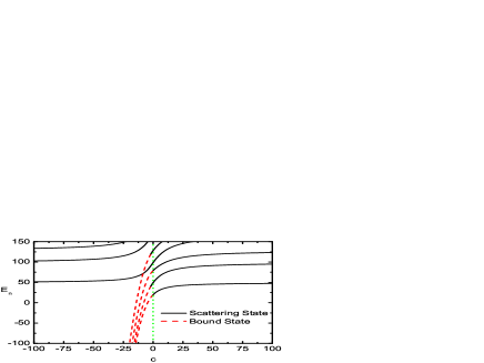
Figure 1: (color online) Energy levels of Bose gas with $N=2$ for different interaction $c$.

For the repulsive interaction ($c>0$) the solutions of Eq. (5) $k_{j}$ are real, while for the attractive interaction ($c<0$) its solutions might be either real or complex. The real solutions correspond to scattering states, which can be obtained by solving Eq. (5). We determine the quantum number $n_{j}$ in the limit of strong interaction ($c\rightarrow\pm\infty$) or the limit of zero interaction ($c\rightarrow 0$). In the former situation the exact wave function can be constructed by means of the Bose-Fermi mapping method from the wave function of $N$ free Fermions GirardeauSTG , i.e., the eigenfunction of single particle in the hard wall trap $sin(j\pi x/L)$ with $j$ being integers. For the ground state $j=1,\cdots,N$ and the excited states are obtained when some $j$ are replaced by the integers greater than $N$. In the ground state of noninteracting limit all Bose atoms shall condense into the ground state of single particle, which gives the exact many body function as $\phi(x_{1},\cdots,x_{N})=\prod_{j}sin(\pi x_{j}/L)$. The wave function of excited states in noninteracting limit, however, takes the form of $\phi(x_{1},\cdots,x_{N})=P\prod_{j}sin(n_{j}\pi x_{j}/L)$, where $P$ is an operator preserving the exchange symmetry of the many body wave function. By comparing these exact wave function with those obtained from Eq. (5), the quantum number $n_{j}$ can be obtained. It is convenient to use the strong interacting limit here. As $c$ approximates to $\pm\infty$ all terms in the summation of Eq. (5) vanish such that the quasimomenta $k_{j}=n_{j}\pi/L$. Comparing the above exact solution we have $n_{j}=j$ ($j=1,\cdots,N$) for the ground state and the excited states correspond to $n_{j}>j$. After deciding the quantum number it is easy to obtain the solution in the limit of $c\rightarrow\pm 0$. As $c$ approximate $0^{+}$ we have $k_{j}=(n_{j}-j+1)\pi/L$ and as $c$ approximate $0^{-}$ we have $k_{j}=(n_{j}+j-1)\pi/L$.

The complex solutions correspond to bound states, which can be obtained by assuming the solutions of complex form $k_{j}=\alpha_{j}+i\Lambda_{j}$ and solving the set of equations of $\alpha_{j}$ and $\Lambda_{j}$. For example, the complex solutions of Bethe ansatz equations for the system of $N=2$ are assumed as $k_{j}=k/2+i\Lambda$ and the Bethe ansatz equations take the formulation of

$$kL = n\pi+2\arctan{\frac{c}{k},}$$

$$\exp\left[2\Lambda L\right] = (-1)^{n}\frac{2\Lambda-c}{2\Lambda+c},$$

where the integer $n\geq 2$ is quantum number and for the ground state $n=2$. As an example, we display the full energy spectrum for $N=2$ in Fig. 1. The scattering states are denoted by solid lines and the bound states are denoted by dashed lines. It is shown that the ground state for repulsive case is scattering state and that for attractive case is bound state. The excited state of attractive Bose gas in the scattering state has been realized experimentally in Ref. Haller . By tuning the 1D interaction constant the Bose atoms evolve from the weakly interacting Thomas-Fermi regime to the strongly repulsive TG regime in which the TG gas was realized, and then by quenching the interaction from the strong repulsion to the strong attraction the scattering states of attractive Bose gas, i.e., the STG gas, was realized. Starting from a stable STG gas, we can further investigate the crossover behavior of the STG gas when one decreases the attractive interaction very slowly to the very weak limit. Through an adiabatically slow change of the attractive interaction, the lowest scattering state of attractive 1D Bose gas in the whole attractive regime could be reached.

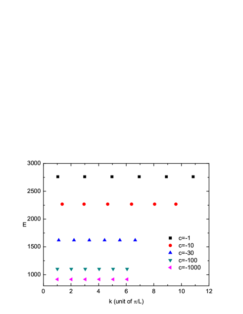
Figure 2: (color online) The quasimomentum distribution and the corresponding energy for the gas with $N=6$ and $c=-1000,-100,-30,-10,0$ (from below to above).

In Fig. 2 we display the quasimomentum distribution and the corresponding energy (longitudinal axis) for the lowest scattering state of the attractive Bose gases with $N=6$ in the full attractive interacting regime. According to Eq. (5) in the limit of STG ($c\rightarrow-\infty$) the solutions of Bethe ansatz equation are equal to those of TG gas ($c\rightarrow+\infty$), i.e., $k_{j}=j\pi/L$ $(j=1,\cdots,N)$. We find that with the decrease of attractive interaction strength, $k_{j}$ tend to distribute with larger and larger space between them although the lowest quasimomentum $k_{1}$ increase first and then decrease. In the limit of noninteracting limit $c\rightarrow 0^{-}$ we have $k_{j}=(2j-1)\pi/L$ $(j=1,\cdots,N)$ and the space between two neighbor $k_{j}$ has evolved from $\pi/L$ ($c=-\infty$) to $2\pi/L$ ($c=0$). The energy of the lowest scattering state increases with the decrease of attractive interaction.

III Properties of the Lowest Scattering States for Attractive Bose Gases

In terms of the lowest scattering state wave function $\Psi\left(x_{1},\cdots,x_{N}\right)$ the important quantity in one dimensional interacting many-body system, the ROBDM, can be formulated as

$$\rho(x,x^{\prime})$$

$$= \frac{N\int_{0}^{L}dx_{2}\cdots dx_{N}\Psi^{\ast}\left(x,x_{2},\cdots,x_{N}\right)\Psi\left(x^{\prime},x_{2},\cdots,x_{N}\right)}{\int_{0}^{L}dx_{1}\cdots dx_{N}\left|\Psi\left(x_{1},x_{2},\cdots,x_{N}\right)\right|^{2}}.$$

The diagonal part of ROBDM gives the expectation values of density distribution $\rho(x)=\rho(x,x^{\prime})|_{x=x^{\prime}}$, and the off-diagonal part gives information of coherent properties of the gas. The Fourier transformation of $\rho(x,x^{\prime})$ gives the momentum distribution

$$n\left(k\right)=\frac{1}{2\pi}\int_{0}^{L}dx\int_{0}^{L}dx^{\prime}\rho(x,x^{\prime})e^{-ik\left(x-x^{\prime}\right)}.$$ (6)

Figure 3: The reduced one body density matrix for the gas with $N=4$ for $c=-1000,-10,-1,0$ (from the left above to the right below).

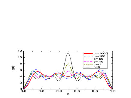
Figure 4: (color online) Density distribution for the gas with $N=4$.

Fig. 3 shows the ROBDM for the lowest scattering state of attractive Bose gas with $N=4$. It deserves to notice that for all attractively interacting strengthes there exists a strong enhancement of the diagonal contribution $\rho(x,x^{\prime})$ along the line $x=x^{\prime}$. In the limit of strong attraction, the system displays the same behavior as TG gases that $\rho(x,x^{\prime})$ reduces rapidly as $|x-x^{\prime}|$ increases. For weaker attraction the off-diagonal part of ROBDM shall increase gradually and we have approximately $\rho(x,L-x)\approx\rho(x,x)$ when the attraction is weak enough. The density distributions of the lowest scattering state for different attractive interacting strength are displayed in Fig. 4. In the strongly attractive limit, it is shown that the density profile of the STG gas of $N$ atoms exhibits the Fermi-like shell structure of $N$-peak similar to the density profile of the TG gas. This is due to the fact that the STG state in the limit of $c\rightarrow-\infty$ and the TG state in the limit of $c\rightarrow\infty$ are actually identical. As the attraction decreases, the density distribution deviates the Fermi-like distribution and the shell structure oscillates more and more dramatically. In the limit of $c$ approaching $0^{-}$ there appear $2N-1$ peaks in the density profile. The atoms tend to populate at the center of the trap with the most probability and the density distribution displays an obvious peak in the center and oscillates in the region away from the center. In the limit of the strong attraction atoms populate in the $N$ lowest eigenstates of single particle so the density profiles show the structure of $N$-peak. As the decrease of attraction atoms populate at higher eigenstates and the peak number shall increase. As $c\rightarrow 0^{-}$, atoms distribute at the $N$ lowest odd states of single particle such that the density profile exhibits $2N-1$ peaks.

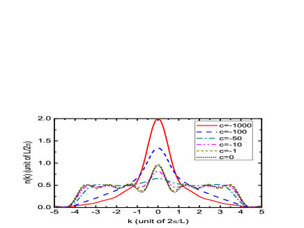
Figure 5: (color online) Momentum distribution for the gas with $N=4$.

The momentum distributions for the lowest scattering state are shown in Fig. 5. For strong attractive interaction, the atoms accumulate in the central regime close to zero momentum and the population distributions decrease rapidly for large momentum, which reflects the statistics of bosonic atoms. With the decrease of attraction the atoms distribute more extensively in higher momentum region and in the strong but finite attractive interaction (e.g. $c=-50$) the atoms distribute widely in the momentum space without an obvious zero-momentum peak. For even weaker attractive interaction, the probability of atoms locating at the zero momentum increases and the momentum distribution develops a prominent peak at zero point $k=0$. Away from the central peak, the momentum distribution starts to display shell structure, which however exhibits distinct feature from the momentum distribution of Fermi gas. It is because the lowest scattering state is an excited state that the Bose atoms populate in higher momentum region.

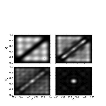
Figure 6: Two-body correlation for $c=-1000,-10,-5,0$ (from the left above to the right below).

It is also interesting to study the two body correlation function defined as

$$g_{2}(x,x^{\prime})$$

$$= \frac{N(N-1)\int_{0}^{L}dx_{3}\cdots dx_{N}\left|\Psi\left(x,x^{\prime},x_{3},\cdots,x_{N}\right)\right|^{2}}{\int_{0}^{L}dx_{1}\cdots dx_{N}\left|\Psi\left(x_{1},x_{2},\cdots,x_{N}\right)\right|^{2}},$$

which denotes the probability that one measurement will find an atom at the point $x$ and the other one at the point $x^{\prime}$. In Fig. 6 we display the two body correlation of lowest scattering state for the Bose gas with $N=4$. It turns out that two atoms with strong attractive interaction would try to avoid each other and try to keep away from each other in certain distance, while as the decrease in attraction the probability of finding two atoms in the adjacent region increase and arrive at the maximum as $c\rightarrow 0$.

IV Summary

In conclusion we have investigated the lowest scattering state of Bose gas in the full attractive interacting regime with Bethe ansatz method. By solving the Bethe ansatz equations numerically the exact wave functions of the lowest scattering state were determined. Based on the wave function we obtain the ROBDM, density profile, momentum distribution and two-body correlation. It is shown that in the STG limit the ROBDM of the lowest scattering state exhibit the same behavior as TG gas. With the decrease of attractive interaction the density distribution evolves from a $N$-peak shell structure to a $(2N-1)$-peak one and Bose atoms are located at the center of the trap with the most probability. The momentum distribution manifests the nature of Bose statistics in the STG limit with an obvious zero-momentum peak. When the attraction keeps on deviating the STG limit the momentum distribution spreads more widely although the most probable position at which the atoms populate is still near the region of zero momentum. The change of the two body correlation function with the decrease in the attractive interaction is also discussed.

- (1) A. Görlitz, J. M. Vogels, A. E. Leanhardt, C. Raman, T. L. Gustavson, J. R. Abo-Shaeer, A. P. Chikkatur, S. Gupta, S. Inouye, T. Rosenband and W. Ketterle, Phys. Rev. Lett. 87, 130402 (2001).
- (2) H. Moritz, T. Stöferle, M. Köhl and T. Esslinger, Phys. Rev. Lett. 91, 250402 (2003).
- (3) B. Paredes, A. Widera, V. Murg, O. Mandel, S. Fölling, I. Cirac, G. V. Shlyapnikov, T. W. Hänsch and I. Bloch, Nature 429, 277 (2004).
- (4) T. Kinoshita, T. Wenger and D. S. Weiss, Science 305, 1125 (2004).
- (5) T. Stöferle, H. Moritz, C. Schori, M. Köhl and T. Esslinger, Phys. Rev. Lett. 92, 130403 (2004).
- (6) E. Haller, M. J. Mark, R. Hart, J. G. Danzl, L. Reichsö llner, V. Melezhik, P. Schmelcher and H. C. Nägerl, Phys. Rev. Lett. 104, 153203 (2010).
- (7) M. Olshanii, Phys. Rev. Lett. 81, 938 (1998).
- (8) T. Bergeman, M. G. Moore and M. Olshanii, Phys. Rev. Lett. 91, 163201 (2003).
- (9) D. S. Petrov, G. V. Shlyapnikov and J. T. M. Walraven, Phys. Rev. Lett. 85, 3745 (2000).
- (10) V. Dunjko, V. Lorent and M. Olshanii, Phys. Rev. Lett. 86, 5413 (2001).
- (11) M. D. Girardeau, J. Math. Phys. (N.Y.) 1, 516 (1960); L. Tonks, Phys. Rev. 50, 955 (1936).
- (12) K. Winkler,G. Thalhammer, F. Lang, R. Grimm, J. Hecker Denschlag, A. J. Daley, A. Kantian, H. P. Büchler and P. Zoller, Nature 441, 853 (2006).
- (13) E. Haller, M. Gustavsson, M. J. Mark, J. G. Danzl, R. Hart, G. Pupillo and H. Näerl, Science 325, 1224 (2009).
- (14) G. E. Astrakharchik, J. Boronat, J. Casulleras and S. Giorgini, Phys. Rev. Lett. 95, 190407 (2005).
- (15) M. T. Batchelor, M. Bortz, X. W. Guan and N. Oelkers, J. Stat. Mech.: Theory Exp. (2005) L10001.
- (16) S. Chen, L. Guan, X. Yin, Y. Hao and X. W. Guan, Phys. Rev. A 81, 031609(R) (2010).
- (17) L. Wang, Y. Hao and S. Chen, Phys. Rev. A 81, 063637 (2010).
- (18) S. Chen, X. W. Guan, X. Yin, L. Guan and M. T. Batchelor, Phys. Rev. A 81, 031608(R) (2010); L. Guan and S. Chen, Phys. Rev. Lett. 105, 175301 (2010); X. Yin, X. W. Guan, M. T. Batchelor, and S. Chen Phys. Rev. A 83, 013602 (2011).
- (19) M. D. Girardeau and G. E. Astrakharchik, Phys. Rev. A 81, 061601(R) (2010); M. D. Girardeau, Phys. Rev. A 82, 011607(R) (2010); M. D. Girardeau, Phys. Rev. A 83, 011601(R) (2011).
- (20) D. Muth and M. Fleischhauer, Phys. Rev. Lett. 105, 150403 (2010).
- (21) M. Kormos, G. Mussardo, and A. Trombettoni Phys. Rev. A 83, 013617 (2011).
- (22) L. Guan, S. Chen, Y. Wang and Z. Q. Ma, Phys. Rev. Lett. 102, 160402 (2009).
- (23) J. N. Fuchs, D. M. Gangardt, T. Keilmann and G.V. Shlyapnikov, Phys. Rev. Lett. 95, 150402 (2005); M. T. Batchelor, M. Bortz, X. W. Guan and N. Oelkers, J. Stat. Mech. P03016 (2006).
- (24) Y. Hao, Y. Zhang, J. Q. Liang and S. Chen, Phys. Rev. A 73, 063617 (2006); Y. Hao, Y. Zhang, X. W. Guan and S. Chen, Phys. Rev. A 79, 033607 (2009).
- (25) M. A. Cazalilla and A. F. Ho, Phys. Rev. Lett. 91, 150403 (2003).
- (26) F. Deuretzbacher, K. Bongs, K. Sengstock and D. Pfannkuche, Phys. Rev. A 75, 013614 (2007); X. Yin, Y. Hao, S. Chen and Y. Zhang,, Phys. Rev. A 78, 013604 (2008).
- (27) Y. Hao and S. Chen, Eur. Phys. J. D 51, 261 (2009).
- (28) M. D. Girardeau and A. Minguzzi, Phys. Rev. Lett. 99, 230402 (2007).
- (29) Alexej I. Streltsov, O. E. Alon and L. S. Cederbaum, Phys. Rev. A 73, 063626 (2006).
- (30) S. Zöllner, H.-D. Meyer, and P. Schmelcher, Phys. Rev. A 74, 063611 (2006); 74, 053612 (2006).
- (31) M. Gaudin, Phys. Rev. A 4, 386 (1971); M. T. Batchelor, X. W. Guan, N. Oelkers and C. Lee, J. Phys. A 38, 7787 (2005).