Distributed NEGF Algorithms for the Simulation of Nanoelectronic Devices with Scattering

Abstract

Through the Non-Equilibrium Green’s Function (NEGF) formalism, quantum-scale device simulation can be performed with the inclusion of electron-phonon scattering. However, the simulation of realistically sized devices under the NEGF formalism typically requires prohibitive amounts of memory and computation time. Two of the most demanding computational problems for NEGF simulation involve mathematical operations with structured matrices called semiseparable matrices. In this work, we present parallel approaches for these computational problems which allow for efficient distribution of both memory and computation based upon the underlying device structure. This is critical when simulating realistically sized devices due to the aforementioned computational burdens. First, we consider determining a distributed compact representation for the retarded Green’s function matrix $G^{R}$. This compact representation is exact and allows for any entry in the matrix to be generated through the inherent semiseparable structure. The second parallel operation allows for the computation of electron density and current characteristics for the device. Specifically, matrix products between the distributed representation for the semiseparable matrix $G^{R}$ and the self-energy scattering terms in $\Sigma^{<}$ produce the less-than Green’s function $G^{<}$. As an illustration of the computational efficiency of our approach, we stably generate the mobility for nanowires with cross-sectional sizes of up to $4.5$nm, assuming an atomistic model with scattering.

1 Introduction

In the absence of electron-phonon scattering, the problem of computing density of states and transmission through the NEGF formalism reduces to a mathematical problem of finding select entries from the inverse of a typically large and sparse block tridiagonal matrix. Although there has been research into numerically stable and computationally efficient serial computing algorithms [1], when analyzing certain device geometries this type of method will result in prohibitive amounts of computation and memory consumption. In [2] a parallel divide-and-conquer algorithm (PDIV) was shown to be effective for NEGF based simulations. Two applications were presented, the atomistic level simulation of silicon nanowires and the two-dimensional simulation of nanotransistors. Alternative, serial computing, NEGF based approaches such as [3] rely on specific problem structure (currently not capable of addressing atomistic models), with computation limitations that again restrict the size of simulation. In addition, the ability to compute information needed to determine current characteristics for devices has not been demonstrated with methods such as [3]. The prohibitive computational properties associated with NEGF based simulation has prompted a transition to wave function based methods, such as those presented in [4]. Given an assumed basis structure the problem translates from calculating select entries from the inverse of a matrix to solving large sparse systems of linear equations. This is an attractive alternative because solving large sparse systems of equations is one of the most well studied problems in applied mathematics and physics. In addition, popular algorithms such as UMFPACK [5] and SuperLU [6] have been constructed to algebraically (based solely on the matrix) exploit problem specific structure in an attempt to minimize the amount of computation. The performance of these algorithms for the wave function based analysis of several silicon nanowires has been examined in [7]. However, for many devices of interest wave function methods are currently unable to address more sophisticated analyses that involve electron-phonon scattering. Thus, there remains a strong need to further develop NEGF based algorithms for the simulation of realistically sized devices considering these general modeling techniques.

When incorporating the effects of scattering into NEGF based simulation, it becomes necessary to determine the entire inverse of the coefficient matrix associated with the device. This substantially increases both the computational and memory requirements. There are a number of theoretical results describing the structure of the inverses of block tridiagonal and block-banded matrices. Representations for the inverses of tridiagonal, banded, and block tridiagonal matrices can be found in [8, 9, 10, 13, 11, 12]. It has been shown that the inverse of a tridiagonal matrix can be compactly represented by two sequences $\{u_{i}\}$ and $\{v_{i}\}$ [14, 15, 16, 17]. This result was extended to the cases of block tridiagonal and banded matrices in [18, 19, 20], where the $\{u_{i}\}$ and $\{v_{i}\}$ sequences generalized to matrices $\{U_{i}\}$ and $\{V_{i}\}$. Matrices that can be represented in this fashion are more generally known as semiseparable matrices [21, 20]. Typically, the computation of parameters $\{u_{i}\}$ and $\{v_{i}\}$ suffers from numerical instability even for modest-sized problems [22]. It is well understood that for matrices arising in many physical applications the $\{u_{i}\}$ and $\{v_{i}\}$ sequences grow exponentially [23, 17] with the index $i$. One approach that has been successful in ameliorating these problems, for the tridiagonal case, is the generator approach shown in [24]. Here, ratios for sequential elements of the $\{u_{i}\}$ and $\{v_{i}\}$ sequences are used as the generators for the inverse of a tridiagonal matrix. Such an approach is numerically stable for matrices of very large sizes. The extension of this generator approach to the general block-tridiagonal matrices was discussed by the same authors in [13]. The authors used the block factorization of the original block-tridiagonal matrix to construct a block Cholesky decomposition of its inverse.

A generator based approach for inversion, typically referred to as the Recursive Green’s Function (RGF) algorithm, was introduced in [1] for NEGF based simulation. It is important to note that the method of [1] requires $3\times$ less memory to compute only the density of states and transmission (in the absence of scattering), when compared to the complete generator representation. In this work, we extend the approach of [2] to consider the computation of a distributed generator representation for the inverse of the block tridiagonal coefficient matrix. We then demonstrate how the distributed generator representation allows for the efficient computation of the electron density and current characteristics of the device. Our parallel algorithms facilitate the simulation of realistically sized devices by utilizing additional computing resources to efficiently divide both the computation time and memory requirements. As an illustration, we stably generate the mobility for $4.5$nm cross-section nanowires assuming an atomistic model with scattering.

2 Inverses of Block Tridiagonal Matrices

A block-symmetric matrix $K$ is block tridiagonal if it has the form

$$K=\begin{pmatrix}A_{1}&-B_{1}\\ -B_{1}^{T}&A_{2}&-B_{2}\\ &\ddots&\ddots&\ddots\\ &&-B_{N_{y}-2}^{T}&A_{N_{y}-1}&-B_{N_{y}-1}\\ &&&-B_{N_{y}-1}^{T}&A_{N_{y}}\\ \end{pmatrix},$$ (1)

where each $A_{i},B_{i}\in\mathbb{R}^{N_{x}\times N_{x}}$. Thus $K\in\mathbb{R}^{N_{y}N_{x}\times N_{y}N_{x}}$, with $N_{y}$ diagonal blocks of size $N_{x}$ each. We will use the notation $K=\mathrm{tri}(A_{1:N_{y}},B_{1:N_{y}-1})$ to represent such a block tridiagonal matrix. The NEGF based simulation of nanowires using the $sp3d5s*$ atomistic tight-binding model with electron-phonon scattering has been demonstrated in [25]. The block tridiagonal coefficient matrix for simulation is constructed in the following way:

$$K=\left(EI-H-\Sigma^{R}_{R}-\Sigma^{R}_{L}-\Sigma^{R}_{S}\right).$$

Here, $E$ is the energy of interest, $H$ is the Hamiltonian containing atomistic interactions, and $\Sigma^{R}_{L}$, $\Sigma^{R}_{R}$, and $\Sigma^{R}_{S}$ are the left and right boundary conditions and self energy scattering terms respectively. In order to calculate the current characteristics for the device we must first form the retarded Greens Function using the fact that $KG^{R}=I$. A standard numerically stable mathematical representation for the inverse of this block tridiagonal matrix is dependent on two sequences of generator matrices $\{g^{\underleftarrow{R}}_{i}\}$,$\{g^{\overrightarrow{R}}_{i}\}$. Here, the terms $\underleftarrow{R}$ and $\overrightarrow{R}$ correspond to the forward and backward propagation through the device. Specifically, we can use the diagonal blocks of the inverse $\{D_{i}\}$ and the generators to describe the inverse a block tridiagonal matrix $K$ in the following manner:

$$G^{R}=\begin{pmatrix}D_{1}&D_{1}g^{\overrightarrow{R}}_{1}&\cdots&D_{1}\prod\limits_{k=1}^{N_{y}-1}g^{\overrightarrow{R}}_{k}\\ g^{\underleftarrow{R}}_{1}D_{1}&D_{2}&\cdots&D_{2}\prod\limits_{k=2}^{N_{y}-1}g^{\overrightarrow{R}}_{k}\\ \vdots&\vdots&\ddots&\vdots\\ (\prod\limits_{k=N_{y}-1}^{1}g^{\underleftarrow{R}}_{k})D_{1}&(\prod\limits_{k=N_{y}-1}^{2}g^{\underleftarrow{R}}_{k})D_{2}&\cdots&D_{N_{y}}\end{pmatrix}.$$ (2)

Where the diagonal blocks of the inverse, $D_{i}$, and the generator sequences satisfy the following relationships:

$$\begin{array}[]{l}g^{\underleftarrow{R}}_{1}=A_{1}^{-1}B_{1},\\ g^{\underleftarrow{R}}_{i}=\left(A_{i}-B_{i-1}^{T}g^{\underleftarrow{R}}_{i-1}\right)^{-1}B_{i},\quad i=2,\ldots,N_{y}-1,\\ \\ g^{\overrightarrow{R}}_{N_{y}-1}=B_{N_{y}-1}A_{N_{y}}^{-1},\\ g^{\overrightarrow{R}}_{i}=B_{i}\left(A_{i+1}-g^{\overrightarrow{R}}_{i+1}B_{i+1}^{T}\right)^{-1},\quad i=N_{y}-2,\ldots,1,\\ \\ D_{1}=\left(A_{1}-g^{\overrightarrow{R}}_{1}B_{1}^{T}\right)^{-1},\\ D_{i+1}=\left(A_{i+1}-g^{\overrightarrow{R}}_{i+1}B_{i+1}^{T}\right)^{-1}\left(I+B_{i}^{T}D_{i}g^{\overrightarrow{R}}_{i}\right),~{}~{}~{}~{}i=1,...,N_{y}-2,\\ D_{N_{y}}=A_{N_{y}}^{-1}\left(I+B_{N_{y}-1}^{T}D_{N_{y}-1}g^{\overrightarrow{R}}_{N_{y}-1}\right).\end{array}$$ (3)

The time complexity associated with determining the parametrization of $G^{R}$ by the above approach is $O(N_{x}^{3}N_{y})$, with a memory requirement of $O(N_{x}^{2}N_{y})$.

2.1 Alternative Approach for Determining the Compact Representation

It is important to note that if the block tridiagonal portion of $G^{R}$ is known, the generator sequences $g^{\overrightarrow{R}}$ and $g^{\underleftarrow{R}}$ can be extracted directly, i.e. without the use of entries from $K$ through the generator expressions (3). Examining closely the block tridiagonal portion of $G^{R}$ we find the following relations:

$$\begin{array}[]{l}D_{i}g^{\overrightarrow{R}}_{i}=P_{i}~{}\implies g^{\overrightarrow{R}}_{i}=D_{i}^{-1}P_{i},\quad i=1,\ldots,N_{y}-1,\\ \\ g^{\underleftarrow{R}}_{i}D_{i}=Q_{i}~{}\implies g^{\underleftarrow{R}}_{i}=Q_{i}D_{i}^{-1},\quad i=1,\ldots,N_{y}-1,\\ \end{array}$$ (4)

where $P_{i}$ denotes the $(i,i+1)$ block entry of $G^{R}$ and $Q_{i}$ denotes the $(i+1,i)$ block entry of $G^{R}$. Therefore, by being able to produce the block tridiagonal portion of $G^{R}$ we have all the information that is necessary to compute the compact representation.

As was alluded to in Section 1, direct techniques for simulation of realistic devices often require prohibitive memory and computational requirements. To address these issues we offer a parallel divide-and-conquer approach in order to construct the compact representation for $G^{R}$, i.e. the framework allows for the parallel inversion of the coefficient matrix. Specifically, we introduce an efficient method for computing the block tridiagonal portion of $G^{R}$ in order to exploit the process demonstrated in (4).

3 Parallel Inversion of Block Tridiagonal Matrices

The compact representation of $G^{R}$ can be computed in a distributed fashion by first creating several smaller sub-matrices $\phi_{i}$. That is, the total number of blocks for the matrix $K$ are divided as evenly as possible amongst the sub-matrices. After each individual sub-matrix inverse has been computed they can be combined in a Radix-2 fashion using the matrix inversion lemma from linear algebra. Figure 1 shows both the decomposition and the two combining levels needed to form the block tridiagonal portion of $G^{R}$, assuming $K$ has been divided into four sub-matrices. In general, if $K$ is separated into $p$ sub-matrices there will be $\log p$ combining levels with a total of $p-1$ combining operations or “steps”. The notation $\phi_{i\sim j}^{-1}$ is introduced to represent the result of any combining step, through the use of the matrix inversion lemma. For example, $\phi_{1\sim 2}^{-1}$ is the inverse of a matrix comprised of the blocks assigned to both $\phi_{1}$ and $\phi_{2}$. It is important to note that using the matrix inversion lemma repeatedly to join sub-matrix inverses will result in a prohibitive amount of memory and computation for large simulation problems. This is due to the fact that at each combining step all entries would be computed and stored. Thus, the question remains on the most efficient way to produce the block tridiagonal portion of $G^{R}$, given this general decomposition scheme for the matrix $K$.

In this work, we introduce a mapping scheme to transform compact representations of smaller matrix inverses into the compact representation of $G^{R}$. The algorithm is organized as follows:

• Decompose the block tridiagonal matrix $K$ into $p$ smaller block tridiagonal matrices.

• Assign each sub-matrix to an individual CPU.

• Independently determine the compact representations associated with each sub-matrix.

• Gather all information that is needed to map the sub-matrix compact representations into the compact representation for $G^{R}$.

• Independently apply the mappings to produce a portion of the compact representation for $G^{R}$ on each CPU.

The procedure described above results in a “distributed compact representation” allowing for reduced memory and computational requirements. Specifically, each CPU will eventually be responsible for the elements from both the generator sequences and diagonal blocks that correspond to the initial decomposition (e.g. if $\phi_{1}$ is responsible for blocks $1,2,~{}\mathrm{and}~{}3$ from the matrix $K$, the mappings will allow for the computation of $g^{\overrightarrow{R}}_{1\ldots 3},~{}g^{\underleftarrow{R}}_{1\ldots 3},~{}\mathrm{and}~{}D_{1\ldots 3}$).

In order to derive the mapping relationships needed to produce a distributed compact representation, it is first necessary to analyze how sub-matrix inverses can be combined to form the complete inverse. Consider the decomposition of the block tridiagonal matrix $K$ into two block tridiagonal sub-matrices and a correction term, demonstrated below:

$$K =\underbrace{\begin{pmatrix}\phi_{1}\\ &\phi_{2}\end{pmatrix}}_{\tilde{K}}~{}~{}+~{}~{}XY,$$

$$\phi_{1} =\mathrm{tri}(A_{1:k},B_{1:k-1}),~{}~{}~{}~{}\phi_{2}=\mathrm{tri}(A_{k+1:N_{y}},B_{k+1:N_{y}-1}),~{}~{}~{}~{}\mathrm{and}$$

$$X =\begin{pmatrix}0&\cdots&-B_{k}^{T}&0&\cdots&0\\ 0&\cdots&0&-B_{k}&\cdots&0\end{pmatrix}^{T},~{}Y=\begin{pmatrix}0&\cdots&0&I&\cdots&0\\ 0&\cdots&I&0&\cdots&0\end{pmatrix}.$$

Figure 1: Decomposition of block tridiagonal matrix $K$ into four sub-matrices, where the shaded blocks correspond to the bridge matrices. The two combining levels follow the individual sub-matrix inversions, where $\phi_{i\sim j}^{-1}$ represents the inverse of divisions $\phi_{i}$ through $\phi_{j}$ from the matrix $K$. Matrix mappings will be used to capture the combining effects and allow for the direct computation of the block tridiagonal portion of $G^{R}$.

Thus, the original block tridiagonal matrix can be decomposed into the sum of a block diagonal matrix (with its two diagonal blocks themselves being block tridiagonal) and a correction term parametrized by the $N_{x}\times N_{x}$ matrix $B_{k}$, which we will refer to as the “bridge matrix”. Using the matrix inversion lemma, we have

$$G^{R}=(\tilde{K}+XY)^{-1}=\tilde{K}^{-1}-(\tilde{K}^{-1}X)\left(I+Y\tilde{K}^{-1}X\right)^{-1}(Y\tilde{K}^{-1}),$$

where

$$\tilde{K}^{-1}X = \begin{pmatrix}-\phi_{1}^{-1}\left(:,k\right)B_{k}&0\\ 0&-\phi_{2}^{-1}\left(:,1\right)B_{k}^{T}\end{pmatrix},$$ (5)

$$\left(I+Y\tilde{K}^{-1}X\right)^{-1} = \begin{pmatrix}I&-\phi_{2}^{-1}\left(1,1\right)B_{k}^{T}\\ -\phi_{1}^{-1}\left(k,k\right)B_{k}&I\end{pmatrix}^{-1},$$

$$Y\tilde{K}^{-1} = \begin{pmatrix}0&\phi_{2}^{-1}\left(:,1\right)^{T}\\ \phi_{1}^{-1}\left(:,k\right)^{T}&0\end{pmatrix},$$

and $\phi_{1}^{-1}\left(:,k\right)$ and $\phi_{2}^{-1}\left(:,1\right)$ denote respectively the last and first block columns of $\phi_{1}^{-1}$ and $\phi_{2}^{-1}$.

This shows that the entries of $\tilde{K}^{-1}$ are modified through the entries from the first rows and last columns of $\phi_{1}^{-1}$ and $\phi_{2}^{-1}$, as well as the bridge matrix $B_{k}$. Specifically, since $\phi_{1}$ is before or “above” the bridge point we only need the last column of its inverse to reconstruct $G^{R}$. Similarly, since $\phi_{2}$ is after or “below” the bridge point we only need the first column of its inverse. These observations were noted in [2], where the authors demonstrated a parallel divide-and-conquer approach to determine the diagonal entries for the inverse of block tridiagonal matrices. We begin by generalizing the method from [2] in order to compute all information necessary to determine the distributed compact representation of $G^{R}$ (3). That is, we would like to create a combining methodology for sub-matrix inverses with two major goals in mind. First, it must allow for the calculation of all information that would be required to repeatedly join sub-matrix inverses, in order to mimic the combining process shown in Figure 1. Second, at the final stage of the combining process it must facilitate the computation of the block tridiagonal portion for the combined inverses. Details pertaining to the parallel computation of $G^{R}$ are provided in Appendix A. The time complexity of the algorithm presented is $O({N_{x}^{3}N_{y}}/{p}+N_{x}^{3}\log p)$, with memory consumption $O\left({N_{x}^{2}N_{y}}/{p}+N_{x}^{2}\right)$. The distribution of the compact representation is at the foundation of an efficient parallel method for calculating the less-than Green’s Function $G^{<}$ and greater-than Green’s Function $G^{>}$.

4 Parallel Computation of the Less-than Green’s Function

The parallel inversion algorithm described in Section 3 not only has advantages in computational and memory efficiency but also facilitates the formulation of a fast, and highly scalable, parallel matrix multiplication algorithm. This plays an important role during the simulation process due to the fact that computation of the less-than Green’s Function requires matrix products with the retarded Green’s Function matrix:

$$G^{<}=G^{R}\Sigma^{<}{G^{R}}^{*}.$$ (6)

$\Sigma^{<}$, which we will refer to as the less-than scattering matrix, is typically assumed to be a block diagonal matrix. We will demonstrate how the distributed compact representation of the semiseparable matrix $G^{R}$ presented in Section 3 can be used to calculate the necessary information from $G^{<}$. Specifically, the electron density for the device will be calculated through the diagonal entries of $G^{<}$ and the current characteristics through the first off-diagonal blocks of $G^{<}$.

4.1 Mathematical Description

Recall that our initial state for this procedure would assume that portions of the block tridiaongal (corresponding to the size and location of the divisions) of $G^{R}$ have been calculated and stored. It is important to note that there are many generator representations for $G^{R}$ and we would like to select a representation that will facilitate efficient calculation of $G^{<}$. For the mathematical operation shown in (6), our starting point will be describing the $k^{\mathrm{th}}$ block row of $G^{R}$ in terms of $D_{i},~{}\left(g^{\overrightarrow{R}}_{i}\right)^{T},~{}\mathrm{and}~{}g^{\underleftarrow{R}}_{i}$, the diagonal blocks and two generator sequences respectively. The following expressions are used to determine the generators from the block tridiagonal of the semiseparable matrix:

$$P_{i} =g^{\underleftarrow{R}}_{i}D_{i+1}\Rightarrow g^{\underleftarrow{R}}_{i}=P_{i}\left(D_{i+1}\right)^{-1},$$

$$Q_{i} =\left(g^{\overrightarrow{R}}_{i}\right)^{T}D_{i}\Rightarrow\left(g^{\overrightarrow{R}}_{i}\right)^{T}=Q_{i}\left(D_{i}\right)^{-1}.$$ (7)

$D_{i},~{}P_{i},~{}\mathrm{and}~{}Q_{i}$, are the diagonal, upper diagonal, and lower diagonal blocks respectively. Thus, the generators $\left(g^{\overrightarrow{R}}_{i}\right)^{T}$ and $g^{\underleftarrow{R}}_{i}$ are used to describe the $k^{\mathrm{th}}$ block row of $G^{R}$ semiseparable matrix in the following way:

$$G^{R}\left(k,:\right)=$$

$$~{}~{}\begin{pmatrix}\prod\limits_{i=k-1}^{1}\left(g^{\overrightarrow{R}}_{i}\right)^{T}D_{1}&\cdots&\left(g^{\overrightarrow{R}}_{k-1}\right)^{T}D_{k-1}&D_{k}&g^{\underleftarrow{R}}_{k}D_{k+1}&\cdots\prod\limits_{i=k}^{N_{y}-1}g^{\underleftarrow{R}}_{i}D_{N_{y}}&\end{pmatrix}$$

This generator representation for $G^{R}$ along with the block diagonal structure of $\Sigma^{<}$ allows for us to express each diagonal block of $G^{<}$ in terms of recursive sequences. Both the forward recursive sequence $g^{\overrightarrow{<}}_{i}$ and backward recursive sequence $g^{\underleftarrow{<}}_{i}$ are dependent on a common sequence of injections terms $J_{i}$ (note: the arrow orientation for $g^{<}$ matches that of $g^{R}$). The relationships between the sequences and the diagonal blocks of $G^{<}$ are shown below:

$$J_{i}=D_{i}\Sigma^{<}_{i}D_{i}^{*},~{}\quad i=1,2,\ldots,N_{y}$$

$$g^{\overrightarrow{<}}_{1}=J_{1}$$

$$g^{\overrightarrow{<}}_{i}=J_{i}+\left(g^{\overrightarrow{R}}_{i-1}\right)^{T}g^{\overrightarrow{<}}_{i-1}\left(g^{\overrightarrow{R}}_{i-1}\right)^{C},~{}\quad i=2,\ldots,N_{y}$$

$$g^{\underleftarrow{<}}_{N_{y}}=J_{N_{y}}$$ (8)

$$g^{\underleftarrow{<}}_{i}=J_{i}+g^{\underleftarrow{R}}_{i}g^{\underleftarrow{<}}_{i+1}\left(g^{\underleftarrow{R}}_{i}\right)^{*},~{}\quad i=N_{y}-1,\ldots,1$$

$$G^{<}(1,1)=g^{\underleftarrow{<}}_{1}$$

$$G^{<}(i,i)=g^{\underleftarrow{<}}_{i}+g^{\overrightarrow{<}}_{i}-J_{i},~{}\quad i=2,\ldots,N_{y}$$

Similar serial recursions have been shown in [1] and [26]. Our strategy in this work is to exploit the distributed compact representation of $G^{R}$ in order to produce these sequences efficiently. That is, we will divide the computation needed to calculate the three sequences $J_{i}$, $g^{\overrightarrow{<}}_{i}$, and $g^{\underleftarrow{<}}_{i}$. into several sub-problems that can be efficiently separated across many processors.

As motivation, if we assume that there are $N_{y}=2N$ blocks, we can define two sub-problems by separating $\Sigma^{<}=\Sigma^{<;1}+\Sigma^{<;2}$, where $\Sigma^{<;1}$ contains blocks $1$ through $N$ and $\Sigma^{<;2}$ contains blocks $N+1$ through $2N$. Then, we can write:

$$G^{<}=G^{r}\Sigma^{<}{G^{r}}^{*}=G^{r}\left(\Sigma^{<;1}+\Sigma^{<;2}\right){G^{r}}^{*}=G^{r}\Sigma^{<;1}{G^{r}}^{*}+G^{r}\Sigma^{<;2}{G^{r}}^{*}=G^{<;1}+G^{<;2}.$$

For this example, we have assumed an equal separation of the diagonal blocks for the scattering matrix $\Sigma^{<}$, i.e. $\Sigma^{<;1}_{i}=0,~{}~{}\forall i>N$. Thus, for the first sub-problem we have:

$$J_{i;1}=D_{i}\Sigma^{<;1}_{i}D_{i}^{*},~{}\quad i=1,2,\ldots,N$$

$$J_{i;1}=0,~{}\quad i=N+1,2,\ldots,2N$$

$$g^{\overrightarrow{<}}_{1;1}=J_{1;1}$$

$$g^{\overrightarrow{<}}_{i;1}=J_{i;1}+\left(g^{\overrightarrow{R}}_{i-1}\right)^{T}g^{\overrightarrow{<}}_{i-1;1}\left(g^{\overrightarrow{R}}_{i-1}\right)^{C},~{}\quad i=2,\ldots,N$$

$$g^{\overrightarrow{<}}_{i;1}=\left(g^{\overrightarrow{R}}_{i-1}\right)^{T}g^{\overrightarrow{<}}_{i-1;1}\left(g^{\overrightarrow{R}}_{i-1}\right)^{C},~{}\quad i=N+1,\ldots,2N$$

$$g^{\underleftarrow{<}}_{i;1}=0,~{}\quad i=2N,\ldots,N+1$$

$$g^{\underleftarrow{<}}_{N;1}=J_{N;1}$$

$$g^{\underleftarrow{<}}_{i;1}=J_{i;1}+g^{\underleftarrow{R}}_{i}g^{\underleftarrow{<}}_{i+1;1}\left(g^{\underleftarrow{R}}_{i}\right)^{*},~{}\quad i=N-2,\ldots,1$$

We then see the following relationships for the second sub-problem:

$$J_{i;2}=0,~{}\quad i=1,2,\ldots,N$$

$$J_{i;2}=D_{i}\Sigma^{<;2}_{i}D_{i}^{*},~{}\quad i=N+1,2,\ldots,2N$$

$$g^{\overrightarrow{<}}_{i;2}=0,~{}\quad i=1,\ldots,N$$

$$g^{\overrightarrow{<}}_{N+1;2}=J_{N+1;2}$$

$$g^{\overrightarrow{<}}_{i;2}=J_{i;2}+\left(g^{\overrightarrow{R}}_{i-1}\right)^{T}g^{\overrightarrow{<}}_{i-1;2}\left(g^{\overrightarrow{R}}_{i-1}\right)^{C},~{}\quad i=N+2,\ldots,2N$$

$$g^{\underleftarrow{<}}_{2N;2}=J_{2N;2}$$

$$g^{\underleftarrow{<}}_{i;2}=J_{i;2}+g^{\underleftarrow{R}}_{i}g^{\underleftarrow{<}}_{i+1;2}\left(g^{\underleftarrow{R}}_{i}\right)^{*},~{}\quad i=2N-1,\ldots,N+1$$

$$g^{\underleftarrow{<}}_{i;2}=g^{\underleftarrow{R}}_{i}g^{\underleftarrow{<}}_{i+1;2}\left(g^{\underleftarrow{R}}_{i}\right)^{*},~{}\quad i=N,\ldots,1$$

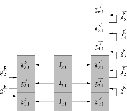
(a) The non-zero matrices that need to be computed for sub-problem 1. The terms that are computed on CPU 1 are shaded.

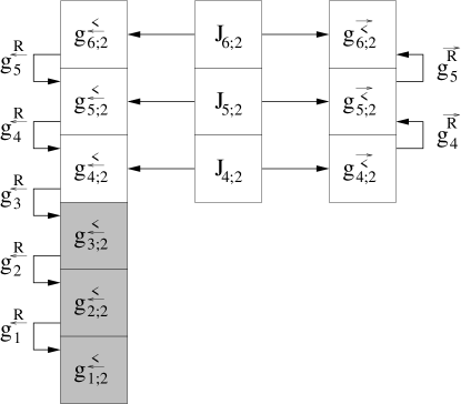
(b) The non-zero matrices that need to be computed for sub-problem 2. The terms that are computed on CPU 2 are shaded.

Figure 2: Distribution of $G^{<}$ computation into two sub-problems across two CPUs.

The recursions for the case of two sub-problems are illustrated in Figure 2 with $N_{y}=2N=6$. Here, the shaded terms in Figure 2(a) and Figure 2(b) represent the terms for each sub-problem that will be computed on CPU 1 and CPU 2 respectively. In summary, the separation of the diagonal blocks, the generator sequences, and the scattering matrix evenly across two computers will result in the following order of operations:

$$\mathrm{CPU~{}1} \mathrm{CPU~{}2}$$

$$\mathrm{Stage~{}I}~{}\quad~{}\quad J_{i;1}=D_{i}\Sigma^{<;1}_{i}D_{i}^{*}, J_{i;2}=D_{i}\Sigma^{<;2}_{i}D_{i}^{*},$$

$$i=1,2,\ldots,N i=N+1,2,\ldots,2N$$

$$\mathrm{Stage~{}II}~{}\quad~{}\quad g^{\overrightarrow{<}}_{1;1}=J_{1;1} g^{\underleftarrow{<}}_{2N;2}=J_{2N;2}$$

$$g^{\overrightarrow{<}}_{i;1}=J_{i;1}+\left(g^{\overrightarrow{R}}_{i-1}\right)^{T}g^{\overrightarrow{<}}_{i-1;1}\left(g^{\overrightarrow{R}}_{i-1}\right)^{C}, g^{\underleftarrow{<}}_{i;2}=J_{i;2}+g^{\underleftarrow{R}}_{i}g^{\underleftarrow{<}}_{i+1;2}\left(g^{\underleftarrow{R}}_{i}\right)^{*},$$

$$i=2,\ldots,N i=2N-1,\ldots,N+1$$

$$\mathrm{Stage~{}III}~{}\quad~{}\quad g^{\underleftarrow{<}}_{i;2}=g^{\underleftarrow{R}}_{i}g^{\underleftarrow{<}}_{i+1;2}\left(g^{\underleftarrow{R}}_{i}\right)^{*}, g^{\overrightarrow{<}}_{i;1}=\left(g^{\overrightarrow{R}}_{i-1}\right)^{T}g^{\overrightarrow{<}}_{i-1;1}\left(g^{\overrightarrow{R}}_{i-1}\right)^{C},$$

$$i=N,\ldots,1 i=N+1,\ldots,2N$$

$$\mathrm{Stage~{}IV}~{}\quad~{}\quad g^{\underleftarrow{<}}_{N;1}=J_{N;1} g^{\overrightarrow{<}}_{N+1;2}=J_{N+1;2}$$

$$g^{\underleftarrow{<}}_{i;1}=J_{i;1}+g^{\underleftarrow{R}}_{i}g^{\underleftarrow{<}}_{i+1;1}\left(g^{\underleftarrow{R}}_{i}\right)^{*}, g^{\overrightarrow{<}}_{i;2}=J_{i;2}+\left(g^{\overrightarrow{R}}_{i-1}\right)^{T}g^{\overrightarrow{<}}_{i-1;2}\left(g^{\overrightarrow{R}}_{i-1}\right)^{C},$$

$$i=N-2,\ldots,1 i=N+2,\ldots,2N$$

If we consider multiplication to be of order $N_{x}^{3}$, then on a single processor the $G^{<}$ calculation would require $3\times(2N_{y})N_{x}^{3}=6N_{y}N_{x}^{3}$ operations. In this case we have four stages, each with $2\times\frac{N_{y}}{2}N_{x}^{3}=N_{y}N_{x}^{3}$ operations. Therefore, using two processors we have reduced the number of multiplications to $4N_{y}N_{x}^{3}$. We now generalize this process and demonstrate further speed-up as both the number of processors and the length of the device increase.

4.2 Parallel Implementation

In order to simplify the presentation of the method, we will assume that the number of sub-problems $p$ evenly divides the total number of blocks $N_{y}=pN$. In general this assumption is not required. We will separate the $G^{<}$ operation evenly into $p$ sub-problems by dividing $\Sigma^{<}=\Sigma^{<;1}+\Sigma^{<;2}+\ldots\Sigma^{<;p}$, where $\Sigma^{<;k}$ contains the $k^{\mathrm{th}}$ portion of the less-than scattering matrix. Given that $\Sigma^{<;k}_{i}=0,~{}~{}\forall i>kN~{}\mathrm{and}~{}i<(k-1)N+1$, the $k^{\mathrm{th}}$ sub-problem will be solved through the following recursions:

$$J_{i;k}=0,~{}\quad i=1,\ldots,(k-1)N$$

$$J_{i;k}=D_{i}\Sigma^{<;k}_{i}D_{i}^{*},~{}\quad i=(k-1)N+1,\ldots,kN$$

$$J_{i;k}=0,~{}\quad i=kN+1,\ldots,pN$$

$$g^{\overrightarrow{<}}_{i;k}=0,~{}\quad i=1,\ldots,(k-1)N$$

$$g^{\overrightarrow{<}}_{i;k}=J_{1;k},~{}\quad i=(k-1)N+1$$

$$g^{\overrightarrow{<}}_{i;k}=J_{i;k}+\left(g^{\overrightarrow{R}}_{i-1}\right)^{T}g^{\overrightarrow{<}}_{i-1;k}\left(g^{\overrightarrow{R}}_{i-1}\right)^{C},~{}\quad i=(k-1)N+2,\ldots,kN$$

$$g^{\overrightarrow{<}}_{i;k}=\left(g^{\overrightarrow{R}}_{i-1}\right)^{T}g^{\overrightarrow{<}}_{i-1;k}\left(g^{\overrightarrow{R}}_{i-1}\right)^{C},~{}\quad i=kN+1,\ldots,pN$$

$$g^{\underleftarrow{<}}_{i;k}=0,~{}\quad i=pN,\ldots,kN+1$$

$$g^{\underleftarrow{<}}_{i;k}=J_{i;k},~{}\quad i=kN$$

$$g^{\underleftarrow{<}}_{i;k}=J_{i;k}+g^{\underleftarrow{R}}_{i}g^{\underleftarrow{<}}_{i+1;k}\left(g^{\underleftarrow{R}}_{i}\right)^{*},~{}\quad i=kN-1,\ldots,(k-1)N+1$$

$$g^{\underleftarrow{<}}_{i;k}=g^{\underleftarrow{R}}_{i}g^{\underleftarrow{<}}_{i+1;k}\left(g^{\underleftarrow{R}}_{i}\right)^{*},~{}\quad i=(k-1)N,\ldots,1$$

So, in a sense by splitting the scattering matrix we have divided the injection sequence $J$ evenly and created two new sub-problem propagating sequences $g^{\overrightarrow{<}}_{i;k}$ and $g^{\underleftarrow{<}}_{i;k}$. However, the sub-problem propagating sequences have the special property that they do not start (are zero) until they reach the indices governed by the sub-problem. This is due to the fact that there are no injection terms for the given sub-problem until these points are reached. In addition, once outside the range of the sub-problem we do not have any additional injection terms in the recursions. Thus, we have a standard two-sided auto-regressive expression where the terms are simply propagated by multiplication with generator matrices.

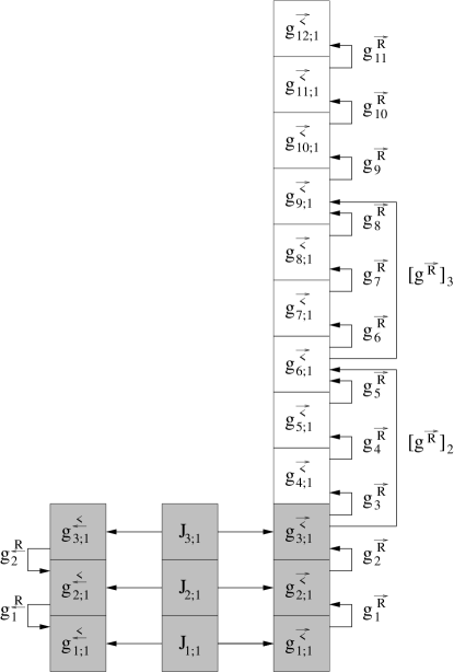
(a) The non-zero matrices that need to be computed for sub-problem 1. The terms that are computed on CPU 1 are shaded.

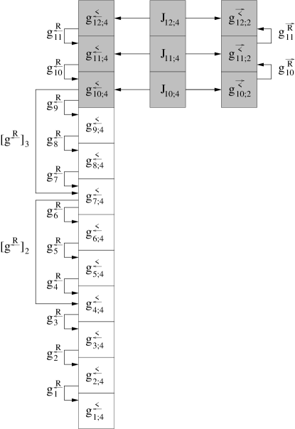
(b) The non-zero matrices that need to be computed for sub-problem 4. The terms that are computed on CPU 4 are shaded.

Figure 3: Distribution of $G^{<}$ computation into four sub-problems across four CPUs.

The recursions for the case of four sub-problems are illustrated in Figure 3 for an example with $N_{y}=4N=12$. Here, the shaded terms in Figure 3(a) and Figure 3(b) represent the terms for each sub-problem that are computed on CPU 1 and CPU 4 respectively. For each sub-problem we introduce two new sequences that will be referred to as ”skip matrices”. Specifically, we define for each processor $k$ two matrices $\left[g^{\underleftarrow{R}}\right]_{k}$ and $\left[g^{\overrightarrow{R}}\right]_{k}^{T}$ that are accumulations of the generator terms stored on the processor. As can be clearly seen from Figure 3 these skip matrices allow for several steps in the recursive process to be preformed through a single operation. Therefore, if the skip matrices are made available to each processor several terms for each sub-problem can be found concurrently. In Figure 3(b), we can see that skip matrices will allow for $g^{\underleftarrow{<}}_{9;4}$, $g^{\underleftarrow{<}}_{6;4}$, and $g^{\underleftarrow{<}}_{3;4}$ to be determined currently by CPUs 3, 2, and 1 respectively.

Given that each sub-problem will produce both a forward and backward propagating sequence it should be clear that CPU $k$ will need to preform computation for $g^{\overrightarrow{<}}$ sequences from sub-problems $\{k+1,k+2,\ldots,p\}$ and $g^{\underleftarrow{<}}$ sequences from sub-problems $\{1,2,\ldots,k-1\}$. However, each $g^{\overrightarrow{<}}$ sequence and $g^{\underleftarrow{<}}$ sequence from other sub-problems may be combined before the generators on that CPU are applied. This is due to the fact that the sequences from each sub-problem will eventually be added together to form $G^{<}=\sum\limits_{k=1}^{p}G^{<;k}$. For the example shown in Figure 3 we see that CPU $1$ will first need to form:

$$g^{\underleftarrow{<}}_{4;4}+g^{\underleftarrow{<}}_{4;3}+g^{\underleftarrow{<}}_{4;2} =\left[g^{\underleftarrow{R}}\right]_{2}\left(\left[g^{\underleftarrow{R}}\right]_{3}g^{\underleftarrow{<}}_{10;4}\left[g^{\underleftarrow{R}}\right]_{3}^{*}+g^{\underleftarrow{<}}_{7;3}\right)\left[g^{\underleftarrow{R}}\right]_{2}^{*}+g^{\underleftarrow{<}}_{4;2},$$

before the required terms for each sub-problem can be calculated. That is, after the lead term for the backward propagating sequence: $\left(g^{\underleftarrow{<}}_{4;4}+g^{\underleftarrow{<}}_{4;3}+g^{\underleftarrow{<}}_{4;2}\right)$ has been computed, the generators governed by CPU 1: $g^{\underleftarrow{R}}_{3}$, $g^{\underleftarrow{R}}_{2}$, and $g^{\underleftarrow{R}}_{1}$, can be applied to fulfill the sub-problem solutions. We now have all the tools necessary to construct a general procedure:

1. Compute the skip products of each generator sequence $g^{\overrightarrow{R}}$ and $g^{\underleftarrow{R}}$, i.e. compute $\left[g^{\underleftarrow{R}}\right]_{k}=\prod\limits_{i=(k-1)N+1}^{kN}{g^{\underleftarrow{R}}_{i}}$ and $\left[g^{\overrightarrow{R}}\right]_{k}^{T}=\prod\limits_{i=kN-1}^{(k-1)N}{\left(g^{\overrightarrow{R}}_{i}\right)^{T}}$, where we will define $\left(g^{\overrightarrow{R}}_{0}\right)^{T}=g^{\underleftarrow{R}}_{N_{y}}=I$.

2. Compute the initial injection and propagation terms for each sub-problem:

   $$J_{i;k}=D_{i}\Sigma^{<;k}_{i}D_{i}^{*},~{}\quad i=(k-1)N+1,\ldots,kN$$

   $$g^{\overrightarrow{<}}_{i;k}=J_{i;k},~{}\quad i=(k-1)N+1$$

   $$g^{\overrightarrow{<}}_{i;k}=J_{i;k}+\left(g^{\overrightarrow{R}}_{i-1}\right)^{T}g^{\overrightarrow{<}}_{i-1;k}\left(g^{\overrightarrow{R}}_{i-1}\right)^{C},~{}\quad i=(k-1)N+2,\ldots,kN$$

   $$g^{\underleftarrow{<}}_{i;k}=J_{i;k},~{}\quad i=kN$$

   $$g^{\underleftarrow{<}}_{i;k}=J_{i;k}+g^{\underleftarrow{R}}_{i}g^{\underleftarrow{<}}_{i+1;k}\left(g^{\underleftarrow{R}}_{i}\right)^{*},~{}\quad i=kN-1,\ldots,(k-1)N+1$$

3. Transfer forward and backward skip products: $\left[g^{\overrightarrow{R}}\right]_{k}^{T}$ and $\left[g^{\underleftarrow{R}}\right]_{k}$, as well as forward and backward lead propagating matrices: $g^{\overrightarrow{<}}_{kN;k}$ and $g^{\underleftarrow{<}}_{(k-1)N+1;k}$, for each sub-problem $k$ to all CPUs. This will be a total of $4pNx^{2}$ entries.

4. CPU $k$ will construct combined lead propagating term for $g^{\underleftarrow{<}}$ sequences from sub-problems $\{k+1,k+2,\ldots,p\}$.

   $$\sum\limits_{j=k+1}^{p}g^{\underleftarrow{<}}_{kN+1;j} =g^{\underleftarrow{<}}_{kN+1;k+1}+\sum\limits_{j=k+2}^{p}\left(\prod\limits_{l=k+1}^{j-1}\left[g^{\underleftarrow{R}}\right]_{l}\right)g^{\underleftarrow{<}}_{(j-1)N+1;j}\left(\prod\limits_{l=j-1}^{k+1}\left[g^{\underleftarrow{R}}\right]_{l}^{*}\right)$$

   CPU $k$ will construct combined lead propagating term for $g^{\overrightarrow{<}}$ sequences from sub-problems $\{1,2,\ldots,k-1\}$.

   $$\sum\limits_{j=1}^{k-1}g^{\overrightarrow{<}}_{(k-1)N;j} =g^{\overrightarrow{<}}_{(k-1)N;k-1}+\sum\limits_{j=1}^{k-2}\left(\prod\limits_{l=k-1}^{j+1}\left[g^{\overrightarrow{R}}\right]_{l}^{T}\right)g^{\overrightarrow{<}}_{jN+1;j}\left(\prod\limits_{l=j+1}^{k-1}\left[g^{\overrightarrow{R}}\right]_{l}^{C}\right)$$

5. Successively multiply by the governed generator terms $g^{\underleftarrow{R}}$ and $g^{\overrightarrow{R}}$ in order fulfill sub-problem solutions.

   $$\sum\limits_{j=k+1}^{p}g^{\underleftarrow{<}}_{i;j} =\left(\prod\limits_{l=i}^{kN}g^{\underleftarrow{R}}_{l}\right)\sum\limits_{j=k+1}^{p}g^{\underleftarrow{<}}_{kN+1;j}\left(\prod\limits_{l=kN}^{i}\left(g^{\underleftarrow{R}}_{l}\right)^{*}\right),$$

   $$i=kN,\ldots,(k-1)N+1.$$

   $$\sum\limits_{j=1}^{k-1}g^{\overrightarrow{<}}_{i;j} =\left(\prod\limits_{l=(i-1)}^{(k-1)N}\left(g^{\overrightarrow{R}}_{l}\right)^{T}\right)\sum\limits_{j=1}^{k-1}g^{\overrightarrow{<}}_{(k-1)N;j}\left(\prod\limits_{l=(k-1)N}^{(i-1)}\left(g^{\overrightarrow{R}}_{l}\right)^{C}\right),$$

   $$i=(k-1)N+1,\ldots,kN.$$

6. Each CPU will combine portions of all sub-problem solutions in order to produce corresponding portion of the diagonal blocks of $G^{<}$ based upon the relationships shown in (4.1).

In order to analyze the computational improvement for the approach we consider the number of multiplications required for each stage. The accumulation of the skip matrices described in Step 1 will result in $2N_{x}^{3}N_{y}/p$ multiplications. The individual sub-problem recursions of Step 2 results in $6N_{x}^{3}N_{y}/p$ multiplications. Step 4 describes how the skip matrices may be applied in order to create the sum for each sub-problem propagating sequence, requiring $2N_{x}^{3}(p-2)$ multiplications. Finally, these two sums must be propagated through each governed generator matrices, requiring $4N_{x}^{3}N_{y}/p$ multiplications. If one is interested in also computing the current characteristics for the device, they may be determined through the off-diagonal blocks of $G^{<}$:

$$G^{<}(i,i+1)=g^{\underleftarrow{<}}_{i+1}\left(g^{\underleftarrow{R}}_{i}\right)^{*}+\left(g^{\overrightarrow{R}}_{i}\right)^{T}g^{\overrightarrow{<}}_{i},~{}\quad i=1,\ldots,N_{y}-1.$$ (9)

As portions of each generator sequence and propagating sequence have been evenly distributed amongst the processors, the resulting computation would be $2N_{x}^{3}N_{y}/p$. Therefore, the total number of multiplications for the approach is $2N_{x}^{3}(p-2)+14N_{x}^{3}N_{y}/p$ compared to $6N_{x}^{3}N_{y}$ for the serial algorithm. Therefore, the speedup of our approach is

$$\frac{p}{2.34+\frac{p(p-2)}{3N_{y}}}$$ (10)

We can clearly see that if $N_{y}>>p$ we will approach a speedup of $p/2.34$.

	$2$nm cross-section				$3$nm cross-section				$4$nm cross-section
$p$	4	8	16	32	4	8	16	32	4	8	16	32
	$35$nm length
$G^{R}$	35.8	21.5	16.2	N/A	411.1	241.4	163.6	N/A	1915.5	1099.7	726.1	N/A
$G^{<}$	22.7	12.7	10.0	N/A	253.7	133.7	81.2	N/A	1159.2	598.5	349.7	N/A
RGF$\times$	1.5	2.7	3.4	N/A	1.4	2.6	4.1	N/A	1.4	2.6	4.2	N/A
	$53$nm length
$G^{R}$	51.4	29.3	19.7	N/A	594.4	331.9	211.4	N/A	2756.1	1523.4	946.4	N/A
$G^{<}$	33.5	18.5	13.8	N/A	380.9	198.5	113.8	N/A	1741.6	887.8	489.1	N/A
RGF$\times$	1.6	2.8	4.0	N/A	1.5	2.7	4.5	N/A	1.4	2.7	4.6	N/A
	$70$nm length
$G^{R}$	67.1	38.8	23.8	17.7	779.0	422.6	255.0	181.3	3601.3	1953.7	1154.5	782.1
$G^{<}$	44.6	24.4	15.8	12.9	507.6	261.5	145.5	103.4	2324.2	1182.2	640.2	408.9
RGF$\times$	1.6	2.8	4.5	5.7	1.5	2.8	4.8	6.8	1.4	2.7	4.9	7.4

Table 1: Runtime comparisons between parallel $G^{R}$ and $G^{<}$ algorithms and serial RGF approach. Silicon nanowires with lengths $35$nm, $53$nm, and $70$nm are examined with cross-sections of $2$nm, $3$nm, and $4$nm. ”RGF$\times$” is the observed speed-up for the combined time. ”N/A” is used for devices that are too short to support the number of CPUs.

5 Results

The parallel $G^{R}$ and $G^{<}$ algorithms have been implemented in C using MPI for inter-processor communication. All computational complexity analyses were performed on a cluster of Intel E5410 processors with $16$GB of shared memory for the $8$ core machines. The OMEN simulator [25] was used to perform simulations for square silicon nanowires employing the $sp3d5s*$ atomistic tight-binding model with electron-phonon scattering. We will begin by demonstrating the computational efficiency of our approach. We will then analyze device characteristics for large cross-section nanowires that have prohibitive memory requirements for the serial RGF approach.

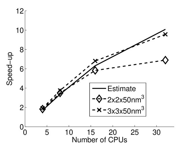
(a) $G^{<}$ speed-up is compared against theoretical estimate from (10) for $50$nm length silicon nanowires.

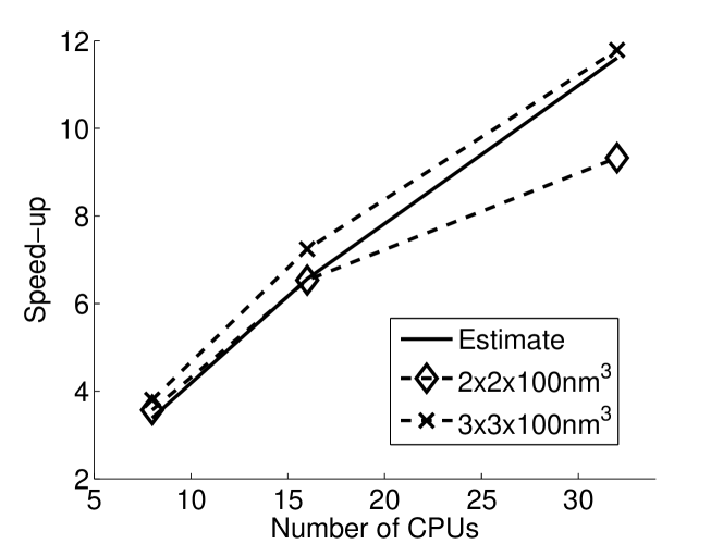
(b) $G^{<}$ speed-up is compared against theoretical estimate from (10) for $100$nm length silicon nanowires.

Figure 4: Verification of theoretical estimate for $G^{<}$ RGF speed-up considering $50$nm and $100$nm length silicon nanowires.

Each NEGF nanowire simulation requires thousands of $G^{R}$, $G^{<}$, and $G^{>}$ computations. For our approach, as well as RGF, the time for each computation will remain constant given that the underlying structure of the Hamiltonian and scattering matrices does not change. In order to analyze the computational benefits of our approach we have examined several different cross-section sizes and lengths of nanowires. Specifically, silicon $\left[100\right]$ nanowires with lengths $35$nm, $53$nm, and $70$nm are examined with cross-sections of $2$nm, $3$nm, and $4$nm. Table 1 shows the runtime for the $G^{R}$ and $G^{<}$ computations (the time needed for $G^{>}$ is identical to that of $G^{<}$). ”RGF$\times$” is the observed speed-up for the combined time of $G^{R}$, $G^{<}$, and $G^{>}$ calculations compared to RGF. ”N/A” is used to for devices that are not long enough to be divided based upon the number of CPUs. We can clearly see that the efficiency of our algorithm improves as both the length and cross-section of the device increase. There are two reasons behind this trend. First, considering a fixed number of processors a longer device will devote less of the total time to sub-problem combining. In addition, as the cross-section size increases the inter-processor communication costs will be a smaller fraction of the total simulation time. We see these effects again when examining Figure 4. Here, we verify the accuracy of the estimated $G^{<}$ scaling trend that was derived in (10). The speed-up over RGF for both $50$nm and $100$nm nanowires are compared against our theoretical estimate. It is important to note that although the speed-up estimate (10) is independent of the cross-section size, effects such as data access time, vector scaling/addition, and inter-processor communication will play a role in determining the efficiency. Thus, in both Figures 4(a) and 4(b) we again see improved efficiency when considering the larger $3$nm cross-section nanowires. In the case of the $3\times 3\times 100$nm³ nanowire we achieve $11.8\times$ speed-up when utilizing $32$ CPUs.

In addition to providing computational improvements, our algorithm facilitates the simulation of larger cross-section devices. If we consider the $4$nm cross-section devices analyzed in Table 1, the RGF method would require between $16$GB and $32$GB of memory for lengths of $35$nm to $70$nm. These devices would not be able to be analyzed without the use of special purpose hardware.

Figure 5: Phonon-limited electron mobility $\mu_{ph}$ as function of the diameter of $\left[100\right]$ oriented circular nanowires at room temperature. The electron density along the channel is homogeneous and set to $n=1e20cm^{-3}$.

As an illustration of the capacity for our algorithm to simulate devices previously viewed to have prohibitive memory requirements, we stably generate the mobility for $4.5$nm cross-section devices with electron-phonon scattering. In order to facilitate complete nanowire simulations we have implemented our algorithm on dual hex-core AMD Opteron 2435 (Istanbul) processors running at 2.6GHz, 16GB of DDR2-800 memory, and a SeaStar 2+ router. As an application, the low-field phonon-limited mobility of electrons $\mu_{ph}$ is calculated in circular nanowires with diameters ranging from $1.5$ to $4.5$nm and transport along the $\left[100\right]$ crystal axis. The ”dR/dL” method [27] and the same procedure as in [28] are used to obtain $\mu_{ph}$. The channel resistance ”R” is computed as function of the nanowire length ”L” and then converted into a mobility. Here, ”L” is set to $35$nm, ”R” is computed in the limit of ballistic transport and in the presence of electron-phonon scattering, and the difference between these two points is considered to evaluate dR/dL. The results are shown in Figure 5. From a numerical perspective, the computation of each Green’s Function, at a given energy, was parallelized on 16 CPUs for all the device structures. As was alluded to above the simulation of these structures would not have been possible (due to memory restrictions) without the decomposition of the device through our parallel methods.

6 Conclusions

In this work we have developed algorithms for parallel NEGF simulation with scattering. The computational benefits of our approach have been demonstrated on large cross-section silicon nanowires. We show improvements of over $11\times$ for the $G^{<}$ and $G^{>}$ computations. In addition, our approach enables simulations without the need for special purpose hardware. This can best be observed through our simulation results for $4.5$nm cross-section silicon nanowires. The algorithms developed in this work are applicable for a wide range of device geometries considering both atomistic and effective-mass models. In addition to offering significant computational improvements over the serial Recursive Green’s Function algorithm, our approach facilitates simulation of realistically sized devices on typical distributed computing hardware.

Appendix A Parallel Computation of the Retarded Green’s Function

In Appendix A we build upon the approach of [2] to consider the computation of a distributed generator representation for $G^{R}$. In Section A.1 we introduce a mapping framework for combining sub-matrices corresponding to subsets of the device structure. This has similarities to the approach presented in [2], where in that case only the diagonal entries of $G^{R}$ were needed to describe the density of states. Section A.2 illustrates how a recursive process can be formulated in order to reconstruct the compact representation of $G^{R}$. This involves several key differences when compared to [2] as significantly more information is required from $G^{R}$. Finally, in Section A.3 the parallel $G^{R}$ algorithm is summarized including an analysis of the computational complexity.

A.1 Matrix Maps

Matrix mappings are constructed in order to eventually produce the block tridiagonal portion of $G^{R}$ while avoiding any unnecessary computation during the combining process. Specifically, we will show that both the boundary block entries (first block row and last block column) and the block tridiagonal entries from any combined inverse $\phi_{i\sim j}^{-1}$ must be attainable (not necessarily computed) for all combining steps. We begin by illustrating the initial stage of the combining process given four divisions, where for simplicity each will be assumed to have $N$ blocks of size $N_{x}$. First, the two sub-matrices $\phi_{1}$ and $\phi_{2}$ are connected through the bridge matrix $B_{N}$ and together they form the larger block tridiagonal matrix $\phi_{1\sim 2}$. By examining Figure 1 it can be seen that eventually $\phi_{1\sim 2}^{-1}$ and $\phi_{3\sim 4}^{-1}$ will be combined and we must therefore produce the boundaries for each combined inverse. From (5) the first block row and last block column of $\phi_{1\sim 2}^{-1}$ can be calculated through the use of an “adjustment” matrix:

$$J =\begin{pmatrix}I&-\phi_{2}^{-1}\left(1,1\right)B_{N}^{T}\\ -\phi_{1}^{-1}\left(N,N\right)B_{N}&I\end{pmatrix}^{-1},$$

as follows:

$$\phi_{1\sim 2}^{-1}(1,:) =\begin{pmatrix}\phi_{1}^{-1}(1,:)&0\end{pmatrix}-\begin{pmatrix}\left[-\phi_{1}^{-1}(1,N)B_{N}J_{12}\phi_{1}^{-1}(:,N)^{T}\right]^{T}\\ \left[-\phi_{1}^{-1}(1,N)B_{N}J_{11}\phi_{2}^{-1}(1,:)\right]^{T}\\ \end{pmatrix}^{T},$$

$$\phi_{1\sim 2}^{-1}(:,2N) =\begin{pmatrix}0&\phi_{2}^{-1}(N,:)\end{pmatrix}^{T}-\begin{pmatrix}\left[-\phi_{2}^{-1}(N,1)B_{N}^{T}J_{22}\phi_{1}^{-1}(:,N)^{T}\right]^{T}\\ \left[-\phi_{2}^{-1}(N,1)B_{N}^{T}J_{21}\phi_{2}^{-1}(1,:)\right]^{T}\\ \end{pmatrix}.$$

In addition, the $r^{\mathrm{th}}$ diagonal block of $\phi_{1\sim 2}^{-1}$ can be calculated using the following relationships for $r\leq N$ :

$$\phi_{1\sim 2}^{-1}(r,r)=\phi_{1}^{-1}(r,r)-\begin{pmatrix}-\phi_{1}^{-1}(r,N)B_{N}J_{12}\phi_{1}^{-1}(r,N)^{T}\end{pmatrix},$$

$$\phi_{1\sim 2}^{-1}(r+N,r+N)=\phi_{2}^{-1}(r,r)-\begin{pmatrix}-\phi_{2}^{-1}(r,1)B_{N}^{T}J_{21}\phi_{2}^{-1}(1,r))\end{pmatrix}^{T},$$

where the $r^{\mathrm{th}}$ off-diagonal block of $\phi_{1\sim 2}^{-1}$ can be calculated using the following relationships:

$$\phi_{1\sim 2}^{-1}(r,r+1)=\phi_{1}^{-1}(r,r+1)-\begin{pmatrix}-\phi_{1}^{-1}(r,N)B_{N}J_{12}\phi_{1}^{-1}(r+1,N)^{T}\end{pmatrix},$$

$$\phi_{1\sim 2}^{-1}(r+N,r+1+N)=\phi_{2}^{-1}(r,r+1)-\begin{pmatrix}-\phi_{2}^{-1}(r+1,1)B_{N}^{T}J_{21}\phi_{2}^{-1}(1,r))\end{pmatrix}^{T},$$

$$r<N,$$

$$\phi_{1\sim 2}^{-1}(r,r+1)=0-\begin{pmatrix}-\phi_{1}^{-1}(r,N)B_{N}J_{11}\phi_{2}^{-1}(1,1)\end{pmatrix},$$

$$r=N.$$

The combination of $\phi_{3}$ and $\phi_{4}$ through the bridge matrix $B_{3N}$ results in similar relationships to those seen above. Thus, in order be able to produce both the boundary and block tridiagonal portions of each combined inverse we assign a total of twelve $N_{x}\times N_{x}$ matrix maps for each sub-matrix $k$. $M_{k;1-4}$ describe effects for the $k^{\mathrm{th}}$ portion of the boundary, $M_{k;5-8}$ describe the effects for a majority of the tridiagonal blocks, while $C_{k;1-4}$, which we will refer to as “cross” maps, can be used to produce the remainder of the tridiagonal blocks.

Initially, for each sub-matrix $i$ the mappings $M_{k;i}=I,~{}~{}k=1,4,$ with all remaining mapping terms set to zero. This ensures that initially the boundary of $\phi_{i\sim i}^{-1}$ matches the actual entries from the sub-matrix inverse, and the modifications to the tridiagonal portion due to combining are all set to zero. By examining the first block row, last block column, and the tridiagonal portion of the combined inverse $\phi_{1\sim 2}^{-1}$ we can see how the maps can be used to explicitly represent all of the needed information. The governing responsibilities of the individual matrix maps are detailed below:

$$\phi_{1\sim 2}^{-1}(1,:)=\begin{pmatrix}\left[M_{1;1}\phi_{1}^{-1}(1,:)+M_{2;1}\phi_{1}^{-1}(:,N)^{T}\right]^{T}\\ \left[M_{1;2}\phi_{2}^{-1}(1,:)+M_{2;2}\phi_{2}^{-1}(:,N)^{T}\right]^{T}\\ \end{pmatrix}^{T},$$

$$\phi_{1\sim 2}^{-1}(:,2N)=\begin{pmatrix}\left[M_{3;1}\phi_{1}^{-1}(1,:)+M_{4;1}\phi_{1}^{-1}(:,N)^{T}\right]^{T}\\ \left[M_{3;2}\phi_{2}^{-1}(1,:)+M_{4;2}\phi_{2}^{-1}(:,N)^{T}\right]^{T}\\ \end{pmatrix},$$

$$\phi_{1\sim 2}^{-1}(r,s)=\phi_{1}^{-1}(r,s)-[\phi_{1}^{-1}(r,1)M_{5;1}\phi_{1}^{-1}(1,s)+\phi_{1}^{-1}(r,1)M_{6;1}\phi_{1}^{-1}(s,N)^{T}+$$

$$\phi_{1}^{-1}(r,N)M_{7;1}\phi_{1}^{-1}(1,s)+\phi_{1}^{-1}(r,N)M_{8;1}\phi_{1}^{-1}(s,N)^{T}],$$ (14)

$$\phi_{1\sim 2}^{-1}(r,s+N)=-[\phi_{1}^{-1}(r,1)C_{1;1}\phi_{2}^{-1}(1,s)+\phi_{1}^{-1}(r,1)C_{2;1}\phi_{2}^{-1}(s,N)^{T}+$$

$$\phi_{1}^{-1}(r,N)C_{3;1}\phi_{2}^{-1}(1,s)+\phi_{1}^{-1}(r,N)C_{4;1}\phi_{2}^{-1}(s,N)^{T}],$$

$$\phi_{1\sim 2}^{-1}(r+N,s+N)=\phi_{2}^{-1}(r,s)-[\phi_{2}^{-1}(r,1)M_{5;2}\phi_{2}^{-1}(1,s)+\phi_{2}^{-1}(r,1)M_{6;2}\phi_{2}^{-1}(s,N)^{T}+$$

$$\phi_{2}^{-1}(r,N)M_{7;2}\phi_{2}^{-1}(1,s)+\phi_{2}^{-1}(r,N)M_{8;2}\phi_{2}^{-1}(s,N)^{T}],$$

$$r,s\leq N,$$

Figure 6: Mapping dependencies when combining $\phi_{1}^{-1}$ and $\phi_{2}^{-1}$ to form $\phi_{1\sim 2}^{-1}$.

It is important to note that all of the expressions (LABEL:eqn:rc_map)-(A.1) can be written into the matrix map framework of (A.1). Figure 6 shows the mapping dependencies for the first block row and last block row (or column since $K$ is symmetric). From (LABEL:eqn:rc_map) we see that both of the block rows are distributed based upon the location of each sub-matrix with respect to the bridge point, i.e. the mapping terms associated with $\phi_{1}^{-1}$ can be used to produce the first portion of the rows while those associated with $\phi_{2}^{-1}$ can be used for the remainder. In fact, this implicit division for the mapping dependencies holds for the block tridiagonal portion of the combined inverses as well, enabling an efficient parallel implementation. Thus, from this point we can deduce that the matrix maps for the first block row (A.1) must be updated in the following manner:

$$M_{1;1}\leftarrow M_{1;1}+(\phi_{1}^{-1}(1,N)B_{N}J_{12})M_{3;1};$$

$$M_{2;1}\leftarrow M_{2;1}+(\phi_{1}^{-1}(1,N)B_{N}J_{12})M_{4;1};$$

$$M_{3;1}\leftarrow(\phi_{1}^{-1}(1,N)B_{N}J_{11})M_{1;2};$$

$$M_{4;1}\leftarrow(\phi_{1}^{-1}(1,N)B_{N}J_{11})M_{2;2};$$

In order to understand these relationships it is important to first recall that the updates to the maps associated with sub-matrix $\phi_{1}$ are dependent on the last block column $\phi_{1}^{-1}(:,N)$. Thus, we see a dependence on the previous state for the last block column $\phi_{1}^{-1}(:,N)$, i.e. the new state of the mapping terms $M_{1;1}$ and $M_{2;1}$ are dependent on the previous state of the mapping terms $M_{3;1}$ and $M_{4;1}$ respectively. Similarly, a dependence on $\phi_{2}^{-1}(1,:)$ results in the new state of the mapping terms $M_{1;2}$ and $M_{2;2}$ being functions of the previous state of the mapping terms $M_{1;2}$ and $M_{1;2}$ respectively. Finally, although some of the mapping terms remain zero after this initial combining step ($M_{2;2}$ for example), the expressions described in (A.1) need to be general enough for the methodology. That is, the mapping expressions must be able to capture combining effects for multiple combing stages, regardless of the position of the sub-matrix with respect to a bridge point. For example, if we consider sub-matrix $\phi_{2}$ for the case seen in Figure 1, during the initial combining step it would be considered a lower problem and for the final combining step it would be considered a upper problem. Alternatively, sub-matrix $\phi_{3}$ would be associated with exactly the opposite modifications. It is important to note that every possible modification process, for the individual mapping terms, is encompassed within this general matrix map framework.

A.2 Recursive Combining Process

In order to formalize the notion of a recursive update scheme we will continue the example from Section A.1. By examining the final combing stage for the case of four divisions, we notice that the approach described in (LABEL:eqn:rc_map)-(A.1) can again be used to combine sub-matrix inverses $\phi_{1\sim 2}^{-1}$ and $\phi_{3\sim 4}^{-1}$, through the bridge matrix $B_{2N}$. The first block row and last block column of $\phi_{1\sim 4}^{-1}$ can be calculated as follows:

$$\phi_{1\sim 4}^{-1}(1,:) =\begin{pmatrix}\phi_{1\sim 2}^{-1}(1,:)&0\end{pmatrix}-\begin{pmatrix}\left[-\phi_{1\sim 2}^{-1}(1,2N)B_{2N}J_{12}\phi_{1\sim 2}^{-1}(:,2N)^{T}\right]^{T}\\ \left[-\phi_{1\sim 2}^{-1}(1,2N)B_{2N}J_{11}\phi_{3\sim 4}^{-1}(1,:)\right]^{T}\\ \end{pmatrix}^{T},$$

$$\phi_{1\sim 4}^{-1}(:,4N) =\begin{pmatrix}0&\phi_{3\sim 4}^{-1}(2N,:)\end{pmatrix}^{T}-\begin{pmatrix}\left[-\phi_{3\sim 4}^{-1}(2N,1)B_{2N}^{T}J_{22}\phi_{1\sim 2}^{-1}(:,2N)^{T}\right]^{T}\\ \left[-\phi_{3\sim 4}^{-1}(2N,1)B_{2N}^{T}J_{21}\phi_{3\sim 4}^{-1}(1,:)\right]^{T}\\ \end{pmatrix},$$

given the adjustment matrix:

$$J =\begin{pmatrix}I&-\phi_{3\sim 4}^{-1}\left(1,1\right)B_{2N}^{T}\\ -\phi_{1\sim 2}^{-1}\left(2N,2N\right)B_{2N}&I\end{pmatrix}^{-1}.$$

In addition, the $r^{\mathrm{th}}$ diagonal block of $\phi_{1\sim 4}^{-1}$ can be calculated using the following relationships:

$$\phi_{1\sim 4}^{-1}(r,r)=\phi_{1\sim 2}^{-1}(r,r)-\begin{pmatrix}-\phi_{1\sim 2}^{-1}(r,2N)B_{2N}J_{12}\phi_{1\sim 2}^{-1}(r,2N)^{T}\end{pmatrix},$$

$$\phi_{1\sim 4}^{-1}(r+2N,r+2N)=\phi_{3\sim 4}^{-1}(r,r)-\begin{pmatrix}-\phi_{3\sim 4}^{-1}(r,1)B_{2N}^{T}J_{21}\phi_{3\sim 4}^{-1}(1,r))\end{pmatrix}^{T},$$

$$r\leq 2N,$$

where the $r^{\mathrm{th}}$ off-diagonal block of $\phi_{1\sim 4}^{-1}$ can be calculated using the following relationships:

$$\phi_{1\sim 4}^{-1}(r,r+1)=\phi_{1\sim 2}^{-1}(r,r+1)-\begin{pmatrix}-\phi_{1\sim 2}^{-1}(r,2N)B_{2N}J_{12}\phi_{1\sim 2}^{-1}(r+1,2N)^{T}\end{pmatrix},$$

$$\phi_{1\sim 4}^{-1}(r+2N,r+1+2N)=\phi_{3\sim 4}^{-1}(r,r+1)-\begin{pmatrix}-\phi_{3\sim 4}^{-1}(r+1,1)B_{2N}^{T}J_{21}\phi_{3\sim 4}^{-1}(1,r))\end{pmatrix}^{T},$$

$$r<2N,$$

$$\phi_{1\sim 4}^{-1}(r,r+1)=0-\begin{pmatrix}-\phi_{1\sim 2}^{-1}(r,2N)B_{2N}J_{11}\phi_{3\sim 4}^{-1}(1,1)\end{pmatrix},$$

$$r=2N.$$

Again, it is important to note that each of the expressions (LABEL:eqn:rc_map_2lvl)-(A.2) are implicitly divided based upon topology. For example, the first $2N$ diagonal blocks of $\phi_{1\sim 4}^{-1}=G^{R}$ can be separated into two groups based upon the size of the sub-matrices $\phi_{1}$ and $\phi_{2}$. That is,

$$\phi_{1\sim 4}^{-1}(r,r)=\phi_{1\sim 2}^{-1}(r,r)-\begin{pmatrix}-\phi_{1\sim 2}^{-1}(r,2N)B_{2N}J_{12}\phi_{1\sim 2}^{-1}(r,2N)^{T}\end{pmatrix},$$

$$r\leq 2N,$$

can be separated for $r\leq N$ as:

$$\phi_{1\sim 4}^{-1}(r,r)=\phi_{1}^{-1}(r,r)-\begin{pmatrix}\left[\phi_{2}^{-1}(N,1)B_{N}^{T}J_{22}\phi_{1}^{-1}(r,N)^{T}\right]^{T}\\ \end{pmatrix}\cdot B_{2N}J_{12}\cdot$$

$$\begin{pmatrix}\left[\phi_{2}^{-1}(N,1)B_{N}^{T}J_{22}\phi_{1}^{-1}(r,N)^{T}\right]\\ \end{pmatrix},$$

$$\phi_{1\sim 4}^{-1}(r+N,r+N)=\phi_{2}^{-1}(r,r)-\begin{pmatrix}\left[\phi_{2}^{-1}(N,r)+\phi_{2}^{-1}(N,1)B_{N}^{T}J_{21}\phi_{2}^{-1}(1,r)\right]^{T}\\ \end{pmatrix}\cdot B_{2N}J_{12}\cdot$$

$$\begin{pmatrix}\left[\phi_{2}^{-1}(N,r)+\phi_{2}^{-1}(N,1)B_{N}^{T}J_{21}\phi_{2}^{-1}(1,r)\right]\\ \end{pmatrix}.$$

Thus, the modifications to the diagonal entries can be written as just a function of the first block row and last block column from the individual sub-matrices, using the matrix map framework introduced in (A.1) for $r\leq N$ :

$$\phi_{1\sim 4}^{-1}(r,r)=\phi_{1}^{-1}(r,r)-\begin{pmatrix}\left[M_{1;1}\phi_{1}^{-1}(1,r)+M_{2;1}\phi_{1}^{-1}(r,N)^{T}\right]^{T}\\ \end{pmatrix}\cdot B_{2N}J_{12}\cdot$$

$$\begin{pmatrix}\left[M_{1;1}\phi_{1}^{-1}(1,r)+M_{2;1}\phi_{1}^{-1}(r,N)^{T}\right]\\ \end{pmatrix},$$

$$\phi_{1\sim 4}^{-1}(r+N,r+N)=\phi_{2}^{-1}(r,r)-\begin{pmatrix}\left[M_{1;2}\phi_{2}^{-1}(1,r)+M_{2;2}\phi_{2}^{-1}(r,N)\right]^{T}\\ \end{pmatrix}\cdot B_{2N}J_{12}\cdot$$

$$\begin{pmatrix}\left[M_{1;2}\phi_{2}^{-1}(1,r)+M_{2;2}\phi_{2}^{-1}(r,N)\right]\\ \end{pmatrix}.$$

Here, the matrix maps are assumed to have been updated based upon the formation of the combined inverses $\phi_{1\sim 2}^{-1}$ and $\phi_{3\sim 4}^{-1}$. Therefore, we can begin to formulate the recursive framework for updating the matrix maps to represent the effect of each combining step.

A.3 Update Scheme for Parallel Inversion and the Distributed Compact Representation

The procedure begins with each division of the problem being assigned to one of $p$ available CPUs. In addition, all of the $p-1$ bridge matrices are made available to each of the CPUs. After the compact representation for each inverse has been found independently, the combining process begins. Three reference positions are defined for the formation of a combined inverse $\phi_{i\sim j}^{-1}$: the “start” position $[\mathtt{st}]=i$, the “stop” position $[\mathtt{sp}]=j$, and the bridge position $[\mathtt{bp}]=\lceil\frac{j-i}{2}\rceil$. Due to the fact that a CPU $t$ will only be involved in the formulation of a combined inverse when $[\mathtt{st}]\leq t\leq[\mathtt{sp}]$ all combining stages on the same level (see Figure 1) can be performed concurrently. When forming a combined inverse $\phi_{i\sim j}^{-1}$, each CPU $[\mathtt{st}]\leq t\leq[\mathtt{sp}]$ will first need to form the adjustment matrix for the combining step. Assuming a bridge matrix $B_{k}$, we begin by constructing four “corner blocks”. If the upper combined inverse is assumed to have $N_{u}$ blocks and the lower to have $N_{l}$, the two matrices need from the upper combined inverse are: $[\mathtt{UR}]=\phi_{[\mathtt{st}]\sim[\mathtt{bp}]}^{-1}(1,N_{u})~{}\mathrm{and}~{}[\mathtt{LR}]=\phi_{[\mathtt{st}]\sim[\mathtt{bp}]}^{-1}(N_{u},N_{u})$, with the two matrices from the lower being: $[\mathtt{UL}]=\phi_{[\mathtt{bp+1}]\sim[\mathtt{sp}]}^{-1}(1,1)~{}\mathrm{and}~{}[\mathtt{LL}]=\phi_{[\mathtt{bp+1}]\sim[\mathtt{sp}]}^{-1}(N_{l},1)$. These matrices can be generated by the appropriate CPU through their respective matrix maps (recall the example shown in Figure 6). Specifically, the CPUs corresponding to the $[\mathtt{st}],~{}[\mathtt{bp}],~{}[\mathtt{bp+1}]~{}\mathrm{and}~{}[\mathtt{sp}]$ divisions govern the required information. The adjustment matrix for the combining step can then be formed:

$$J =\begin{pmatrix}I&-[\mathtt{UL}]B_{k}^{T}\\ -[\mathtt{LR}]B_{k}&I\end{pmatrix}^{-1}.$$

After the adjustment matrix has been calculated the process of updating the matrix maps can begin. For any combining step, the cross maps each CPU $t$ must be updated first:

$$\mathrm{if}~{}~{}(t<[\mathtt{bp}])~{}~{}\mathrm{then}$$

$$~{}~{}C_{1}\leftarrow C_{1}-M_{3;t}^{T}(B_{k}J_{12})M_{3;t+1};$$

$$~{}~{}C_{2}\leftarrow C_{2}-M_{3;t}^{T}(B_{k}J_{12})M_{4;t+1};$$

$$~{}~{}C_{3}\leftarrow C_{3}-M_{4;t}^{T}(B_{k}J_{12})M_{3;t+1};$$

$$~{}~{}C_{4}\leftarrow C_{4}-M_{4;t}^{T}(B_{k}J_{12})M_{4;t+1};$$

$$\mathrm{elseif}~{}~{}(t==[\mathtt{bp}])~{}~{}\mathrm{then}$$ (18)

$$~{}~{}C_{1}\leftarrow C_{1}-M_{3;t}^{T}(B_{k}J_{11})M_{1;t+1};$$

$$~{}~{}C_{2}\leftarrow C_{2}-M_{3;t}^{T}(B_{k}J_{11})M_{2;t+1};$$

$$~{}~{}C_{3}\leftarrow C_{3}-M_{4;t}^{T}(B_{k}J_{11})M_{1;t+1};$$

$$~{}~{}C_{4}\leftarrow C_{4}-M_{4;t}^{T}(B_{k}J_{11})M_{2;t+1};$$

$$\mathrm{elseif}~{}~{}(t<[\mathtt{sp}])~{}~{}\mathrm{then}$$

$$~{}~{}C_{1}\leftarrow C_{1}-M_{1;t}^{T}(B_{k}^{T}J_{21})M_{1;t+1};$$

$$~{}~{}C_{2}\leftarrow C_{2}-M_{1;t}^{T}(B_{k}^{T}J_{21})M_{2;t+1};$$

$$~{}~{}C_{3}\leftarrow C_{3}-M_{2;t}^{T}(B_{k}^{T}J_{21})M_{1;t+1};$$

$$~{}~{}C_{4}\leftarrow C_{4}-M_{2;t}^{T}(B_{k}^{T}J_{21})M_{2;t+1};$$

Notice that the cross maps for CPU $t$ are dependent on information from its neighboring CPU $t+1$. This information must be transmitted and made available before the cross updates can be performed. Next, updates to the remaining eight matrix maps can be separated into two categories. The updates to the matrix maps for the upper sub-matrices $(t\leq[\mathtt{bp}])$, are summarized below:

$$M_{5;t}\leftarrow M_{5;t}-M_{3;t}^{T}(B_{k}J_{12})M_{3;t};$$

$$M_{6;t}\leftarrow M_{6;t}-M_{3;t}^{T}(B_{k}J_{12})M_{4;t};$$

$$M_{7;t}\leftarrow M_{7;t}-M_{4;t}^{T}(B_{k}J_{12})M_{3;t};$$

$$M_{8;t}\leftarrow M_{8;t}-M_{4;t}^{T}(B_{k}J_{12})M_{4;t};$$ (19)

$$M_{1;t}\leftarrow M_{1;t}+([\mathtt{UR}]B_{k}J_{12})M_{3;t};$$

$$M_{2;t}\leftarrow M_{2;t}+([\mathtt{UR}]B_{k}J_{12})M_{4;t};$$

$$M_{3;t}\leftarrow([\mathtt{LL}]^{T}B_{k}^{T}J_{22})M_{3;t};$$

$$M_{4;t}\leftarrow([\mathtt{LL}]^{T}B_{k}^{T}J_{22})M_{4;t};$$

The updates to the matrix maps for the lower sub-matrices $(t>[\mathtt{bp}])$, will be:

$$M_{5;t}\leftarrow M_{5;t}-M_{1;t}^{T}(B_{k}^{T}J_{21})M_{1;t};$$

$$M_{6;t}\leftarrow M_{6;t}-M_{1;t}^{T}(B_{k}^{T}J_{21})M_{2;t};$$

$$M_{7;t}\leftarrow M_{7;t}-M_{2;t}^{T}(B_{k}^{T}J_{21})M_{1;t};$$

$$M_{8;t}\leftarrow M_{8;t}-M_{2;t}^{T}(B_{k}^{T}J_{21})M_{2;t};$$ (20)

$$M_{3;t}\leftarrow M_{3;t}+([\mathtt{LL}]^{T}B_{k}^{T}J_{21})M_{1;t};$$

$$M_{4;t}\leftarrow M_{4;t}+([\mathtt{LL}]^{T}B_{k}^{T}J_{21})M_{2;t};$$

$$M_{1;t}\leftarrow([\mathtt{UR}]B_{k}J_{11})M_{1;t};$$

$$M_{2;t}\leftarrow([\mathtt{UR}]B_{k}J_{11})M_{2;t};$$

The above procedure, shown in (18)-(20), for modifying the matrix maps can be recursively repeated for each of the combining stages beginning with the lowest level of combining the individual sub-matrix inverses.

On completion the maps can then be used to generate the block tridiagonal entries of $G^{R}$. This subsequently allows for the computation of the generator sequences for $G^{R}$, via the relationships shown in (4), in a purely distributed fashion. The time complexity of the algorithm presented is $O({N_{x}^{3}N_{y}}/{p}+N_{x}^{3}\log p)$, with memory consumption $O\left({N_{x}^{2}N_{y}}/{p}+N_{x}^{2}\right)$. The first term $({N_{x}^{3}N_{y}}/{p})$ in the computational complexity arises from the embarrassingly parallel nature of both determining the generator sequences and applying the matrix maps to update the block tridiagonal portion of the inverse. The second term $(N_{x}^{3}\log p)$ is dependent on the number of levels needed to gather combining information for $p$ sub-matrix inverses. Similarly, the first term in the memory complexity is due to the generator sequences and diagonal blocks, and the second represents the memory required for the matrix maps of each sub-problem governed.

References

• [1] A. Svizhenko, M. P. Anantram, T. R. Govindan, B. Biegel, and R. Venugopal. Two-dimensional quantum mechanical modeling of nanotransistors. Journal of Applied Physics, 91(4):2343–2354, 2002.
• [2] S. Cauley, J. Jain, C.-K. Koh, and V. Balakrishnan. A scalable distributed method for quantum-scale device simulation. Journal of Applied Physics, 101(123715), 2007.
• [3] S. Li, S. Ahmed, G. Klimeck, and E. Darve. Computing entries of the inverse of a sparse matrix using the find algorithm. Journal of Computational Physics, 227(22):9408–9427, 2008.
• [4] M. Stadele, R. Tuttle, and K. Hess. Tunneling through ultrathin sio2 gate oxides from microscopic models. Journal of Applied Physics, 89(1):348–363, 2001.
• [5] Timothy A. Davis. Algorithm 832: Umfpack v4.3—an unsymmetric-pattern multifrontal method. ACM Transactions on Mathematical Software, 30(2):196–199, 2004.
• [6] James W. Demmel, Stanley C. Eisenstat, John R. Gilbert, Xiaoye S. Li, and Joseph W. H. Liu. A supernodal approach to sparse partial pivoting. SIAM J. Matrix Analysis and Applications, 20(3):720–755, 1999.
• [7] T.B. Boykin, M. Luisier, and G. Klimeck. Multiband transmission calculations for nanowires using an optimized renormalization method. Phys. Rev, B 77:165318, 2008.
• [8] K. Bowden. A direct solution to the block tridiagonal matrix inversion problem. International Journal of General Systems, 15:185–198, 1989.
• [9] B. Bukhberger and G. A. Emel’yanenko. Methods of inverting tridiagonal matrices. Computational Mathematics and Mathematical Physics, 13:10–20, 1973.
• [10] E. M. Godfrin. A method to compute the inverse of an n-block tridiagonal quasi-hermitian matrix. Journal of Physics:Condensed Matter, 3:7843–7848, 1991.
• [11] T. Oohashi. Some representation for inverses of band matrices. TRU Mathematics, 14:39–47, 1978.
• [12] T. Torii. Inversion of tridiagonal matrices and the stability of tridiagonal systems of linear equations. Technology Reports of the Osaka University, 16:403–414, 1966.
• [13] G. Meurant. A review on the inverse of symmetric block tridiagonal and block tridiagonal matrices. SIAM Journal on Matrix Analysis and Applications, 13(3):707–728, 1992.
• [14] E. Asplund. Inverses of matrices $a_{ij}$ which satisfy $a_{ij}=0$ for $j>i+p$. Mathematica Scandinavica, 7:57–60, 1959.
• [15] S.O. Asplund. Finite boundary value problems solved by green’s matrix. Mathematica Scandinavica, 7:49–56, 1959.
• [16] R. Bevilacqua, B. Codenotti, and F. Romani. Parallel solution of block tridiagonal linear systems. Linear Algebra Appl., 104:39–57, 1988.
• [17] R. Nabben. Decay rates of the inverses of nonsymmetric tridiagonal and band matrices. SIAM Journal on Matrix Analysis and Applications, 20(3):820–837, 1999.
• [18] F. Romani. On the additive structure of inverses of banded matrices. Linear Algebra Appl., 80:131–140, 1986.
• [19] P. Rozsa. On the inverse of band matrices. Integral Equations and Operator Theory, 50:82–95, 1987.
• [20] P. Rozsa, R. Bevilacqua, P. Favati, and F. Romani. On the inverse of block tridiagonal matrices with applications to the inverses of band matrices and block band matrices. Operator Theory: Advances and Applications, 40:447–469, 1989.
• [21] P. Rozsa. Band matrices and semi-separable matrices. Colloquia Mathematica Societatis Janos Bolyai, 50:229–237, 1986.
• [22] P. Concus and Meurant G. On computing INV block preconditionings for the conjugate gradient method. BIT, 26:493–504, 1986.
• [23] S. Demko, W. F. Moss, and Smith P. W. Decay rates for inverses of band matrices. Mathematics of Computation, 43:491–499, 1984.
• [24] P. Concus, G. H. Golub, and Meurant G. Block preconditionings for the conjugate gradient method. SIAM Journal on Scientific Computing, 6:220–252, 1985.
• [25] M. Luisier and G. Klimeck. Atomistic full-band simulations of si nanowire transistors with electron-phonon scattering. Phys. Rev, B 80:155430, 2009.
• [26] J. Jain, S. Cauley, H. Li, C.-K. Koh, and V. Balakrishnan. Numerically stable algorithms for inversion of block tridiagonal and banded matrices, submitted for consideration. Purdue ECE Technical Report (1358), 2007.
• [27] K. Rim, S. Narasimha, M. Longstreet, A. Mocuta, and J. Cai. Low field mobility characteristics of sub-100 nm unstrained and strained Si MOSFETs. IEDM Tech. Dig., 43-46 (2002).
• [28] M. Luisier. Phonon-limited and effective low-field mobility in n- and p-type [100]-, [110]-, and [111]-oriented Si nanowire transistors. Appl. Phys. Lett., 98, 032111 (2011).