A Robust Approach to Constraining Dark Matter Properties with Gamma-Ray Data

Abstract

Photons produced in the annihilations of dark matter particles can be detected by gamma-ray telescopes; this technique of indirect detection serves as a cornerstone of the upcoming assault on the dark matter paradigm. The main obstacle to the extraction of information about dark matter from the annihilation photons is the presence of large and uncertain gamma-ray backgrounds. We present a new technique for using gamma-ray data to constrain the properties of dark matter that makes minimal assumptions about the dark matter and the backgrounds. The technique relies on two properties of the expected signal from annihilations of the smooth dark matter component in our galaxy: 1) it is approximately rotationally symmetric around the axis connecting us to the Galactic Center, and 2) variations from the mean signal are uncorrelated from one pixel to the next. We apply this technique to recent data from the Fermi telescope to generate constraints on the dark matter mass and cross section for a variety of annihilation channels. We quantify the uncertainty introduced into our constraints by uncertainties in the halo profile and by the possibility that the halo is triaxial. The resultant constraint, the flux $F\leq 4.5\times 10^{-6}$ cm^-2 s^-1 sr^-1 for energies between 1 and 100 GeV at an angle $15^{\circ}$ away from the Galactic Center, translates into an upper limit on the velocity weighted annihilation cross section of order $10^{-25}$ cm³ s^-1 depending on the annihilation mode.

I Introduction

Evidence for the existence of non-baryonic dark matter has been accumulating for many decades. Combined constraints from measurements of anisotropies in the cosmic microwave background radiation, the shape of the galaxy power spectrum, and the Hubble constant fix both the total matter and the baryon densities, indicating that non-baryonic dark matter makes up 85% of the matter density of the universe Jarosik et al. (2010). Despite the preponderance of evidence for its existence, however, little is known about the identity of the dark matter. One way to glean information about the properties of this mysterious substance is through indirect detection, the observation of the annihilation products of dark matter particles.

Indirect detection is an attractive prospect for several reasons. Its primary advantage is that, while dark matter itself is very difficult to detect, the annihilation products of dark matter particles may be easily detectable. If photons are produced in dark matter annihilations, for instance, existing telescopes can detect them. Another attractive feature of indirect detection is that the velocity-weighted, thermally averaged annihilation cross section of the dark matter, $\left<\sigma v\right>$, which governs the expected indirect detection signal, is constrained if the dark matter is a thermal relic. Additionally, indirect detection has the potential to reveal information about the distribution of dark matter beyond our local environment. For these and other reasons, indirect detection nicely compliments the other techniques that may be used to identify dark matter: direct detection and collider searches Bergstrom et al. (2010). It is likely that all three techniques will be necessary for a definitive identification of the dark matter.

The present is an exciting time for indirect detection as a number of experiments are currently underway that are capable of detecting a signal from dark matter annihilations. Neutrino detectors such as IceCube and AMANDA Landsman and Icecube Collaboration (2007), air Cherenkov detectors such as H.E.S.S. Horns and H.E.S.S. collaboration (2008) and VERITAS Holder et al. (2006), cosmic ray detectors such as PAMELA Picozza et al. (2007), and space based  $\gamma$-ray telescopes such as the Fermi Gamma-Ray Space Telescope (FGST) Atwood et al. (2009) are all poised to make important contributions to the indirect detection of dark matter.

In this paper, we focus on the possibility of using  $\gamma$-ray data taken by the Large Area Telescope (LAT) on board the FGST to constrain the properties of dark matter. The LAT is a wide field, pair conversion  $\gamma$-ray telescope that covers an energy range from about 20 MeV to 300 GeV Atwood et al. (2009). Gamma-rays are particularly well suited for indirect detection because they are relatively easy to detect, they are produced in many models of dark matter annihilation, and they propagate through the universe with small optical depth (especially at low energies).

Unfortunately, although  $\gamma$-rays may in principle contain significant information about dark matter, the process of extracting this information is severely complicated by the presence of large and uncertain backgrounds to the dark matter signal. The primary challenge of indirect detection using  $\gamma$-rays is therefore to extract a signal which may be hidden in backgrounds that are larger by orders of magnitude. Two primary features of the detected photons are their energy and arrival direction. A number of studies have used these two features to extract the dark matter signal from the background. For example, Ref. Abdo et al. (2010a) used only energy information, while Ref. Zaharijas et al. (2010) and Ref. Hooper and Goodenough (2010) used both the spectral and angular distribution information. Given the photon counts, derived quantities can also be used to distinguish the signal from the backgrounds. The probability distribution function (PDF) has been proposed as a discriminant by a number of groups Lee et al. (2009); Dodelson et al. (2009); Baxter et al. (2010). Anisotropy of the distribution, especially when combined with spectral information, has also been proposed as a powerful way of extracting the signal Siegal-Gaskins and Pavlidou (2009); Hensley et al. (2010).

Here we propose a new and robust approach for constraining dark matter from  $\gamma$-ray data that uses only the angular distribution of the photons. We rely on two important aspects of the dark matter signal to help separate it from backgrounds. First, part of the expected signal from dark matter in our galaxy is smooth (i.e. variations from the mean flux in nearby pixels are uncorrelated). Second, the dark matter signal comes from a nearly spherically symmetric halo, so the signal is azimuthally symmetric about the axis connecting us to the center of our Galaxy. This is in sharp contrast to the backgrounds, which are heavily concentrated near the disk of the Galaxy. More generally, astrophysical backgrounds have different morphologies and may be clumped (i.e. variations from the mean flux may be correlated in nearby pixels). These differences between the signal and the backgrounds allow us to remove some of the contribution from the backgrounds to place an interesting limit on the dark matter. The approach, which we call a Ring Analysis, makes very minimal assumptions about the nature of the signal and no assumptions about the backgrounds. Therefore, this approach is very conservative and will lead to robust limits on the properties of the dark matter.

In §II we describe the way we processed the Fermi LAT data to generate photon count and exposure maps. In §III we present the Ring Analysis technique that we have developed for constraining the presence of an azimuthally symmetric signal on the sky. Consider an annulus centered on the axis connecting us to the Galactic Center, identified by the angle $\psi$ between this axis and the annulus. The Ring Analysis results in an upper limit on any contribution to the flux that is uniform in this annulus. Fig. 4 presents these upper limits on the uniform flux from the Fermi LAT data. Transforming these upper limits into constraints on the properties of dark matter particles requires a number of steps and assumptions. These, and in particular the uncertainties involved, are discussed in §IV. Our conclusions are presented in §V.

II Data

The Fermi LAT is a pair conversion  $\gamma$-ray detector that operates roughly in the energy range from 20 MeV to 300 GeV. A scintillating anti-coincidence detector allows for the rejection of contaminating high energy particle events. The specifications of the detector are described in detail in Ref. Atwood et al. (2009). Our analysis is based on LAT data downloaded in the form of weekly all-sky releases from the Fermi Science Support Center website at http://fermi.gsfc.nasa.gov/ssc/data/.

Even with the on-board anti-coincidence detector there is a residual background of particles that are misclassified as  $\gamma$-rays by the LAT detectors. This poses a challenge for our analysis because these misinterpreted cosmic rays constitute a potentially large and uncertain background. The Fermi collaboration has made public the DataClean event class which implements several data cuts to minimize cosmic ray contamination as well as improved particle background and instrument modeling. Their data selection techniques and event modeling are described in Ref. Abdo et al. (2010b). We restrict our analysis to only the events labeled as DataClean and use the corresponding P6_V3_DATACLEAN instrument response function to calculate exposure maps.

Following Ref. Abdo et al. (2010b), we confine our analysis to those events coming from zenith angles $<100^{\circ}$ in order to reduce contamination by  $\gamma$-rays produced in cosmic ray interactions with the Earth’s atmosphere. The resulting data set amounts to an exposure of roughly $7\times 10^{10}{\,{\rm cm}^{2}}\rm{s}$ across the sky covering a date range from 2008-08-04 to 2010-12-07.

We produce photon count and exposure maps using the GaDGET package, a set of software routines designed for use with the LAT data by the Fermi collaboration Ackermann et al. (2008). In generating the maps, the data were divided into 29 energy bins between 1 GeV and 100 GeV, logarithmically spaced in energy. This restriction in energy was chosen because the LAT performance is well characterized in this energy range. Because the generation of these maps is computationally intensive, the data were processed in parallel on the Fulla computing cluster at Fermilab. The maps generated using the GaDGET software were then converted to the HEALPix isolatitude pixelization scheme with $N_{\rm{side}}=64$, corresponding to a pixel size of roughly $(1^{\circ})^{2}$ (comparable to the width of the point spread function (PSF) of Fermi at the lowest energy we consider). Fig. 1 shows the resulting all-sky  $\gamma$-ray map in the energy range $1\,{\rm GeV}\,<E<100\,{\rm GeV}\,$.

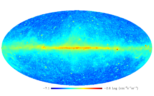
Figure 1: All-sky map of the  $\gamma$-ray flux between 1 GeV and 100 GeV as measured by the FGST with an exposure of roughly $7\times 10^{10}{\,{\rm cm}^{2}}\rm{s}$.

III Ring Analysis

III.1 Overview

The Ring Analysis technique that we develop in this paper is a method for constraining the presence of a signal on the sky that satisfies two requirements: 1) it is azimuthally symmetric, and 2) variations from the mean signal at any zenith angle are uncorrelated from one pixel to the next. As we discuss in §IV, the annihilation signal from smooth dark matter is expected to satisfy these two requirements, and we can quantify the extent to which the signal deviates from these conditions. In this section, however, we make no reference to the nature of the signal itself.

A consequence of these two features is that the signal in each pixel of a ring of constant $\psi$ (where $\psi$ is the zenith angle) can be considered to be drawn independently from some underlying distribution. In the statistical literature, such a signal is referred to as independent and identically distributed, or i.i.d. The constraint will be on the amplitude of any i.i.d. component of the data. In the case of interest, the backgrounds dwarf the signal and the background flux in each pixel may depend on nearby pixels and may vary as a function of the angle transverse to $\psi$, which we label $\phi$.

Consider a ring on the sky of constant $\psi$ defined by $\psi_{i}-\Delta\psi_{i}/2<\psi<\psi_{i}+\Delta\psi_{i}/2$, where $\psi_{i}$ labels the central $\psi$ of the $i$th ring, and $\Delta\psi_{i}$ is its angular width. Since we have divided the sky into pixels, we define $F_{i}(\phi_{j})$ to be the flux in the $j$th pixel (labeled by its azimuth angle $\phi_{j}$) of ring $i$. We assume that the pixels have been sorted in terms of $\phi_{j}$ so that, for example, pixels $j$ and $j+1$ appear adjacent to each other on the sky; such sorting preserves any non-i.i.d. component of the data. The flux $F_{i}(\phi_{j})$ receives contributions from an i.i.d. component due to the signal, $F_{i,S}(\phi_{j})$, and contributions from some possibly non-i.i.d.  components due to the backgrounds, $F_{i,B}(\phi_{j})$ (see upper panel of Fig. 2 for an illustration). Our goal is to obtain an upper limit on the mean contribution from the signal.

Figure 2: An illustration of the terms defined in the text for the case of the data from the Fermi telescope. Top panel: The flux in a ring of constant $\psi_{i}$, $F_{i}(\phi_{j})$, as a function of $\phi$, the angle transverse to $\psi$. For the purposes of illustration, we have chosen a ring centered at $\psi_{i}=15^{\circ}$ of width $6^{\circ}$. The energy of the photons has been restricted to $1\,{\rm GeV}\,<E<100\,{\rm GeV}\,$. The increase in flux at $\phi\approx\pm 90^{\circ}$ is due to the galactic plane. The dashed line illustrates the maximum flux that is consistent with the the data being i.i.d. as determined by the BDS test. Bottom Panel: The function $G_{i}(\phi_{j},F^{T}_{i})$ obtained by dropping all pixels with flux above the threshold $F^{T}_{i}$ in the top panel. This new set of fluxes is inconsistent with an i.i.d. sequence; a slightly lower value of $F^{T}_{i}$ would produce a $G_{i}$ that is consistent with an i.i.d. sequence. Therefore, the chosen value of $F^{T}$ is the strongest constraint on the i.i.d. flux in this ring.

Consider the fluxes in all pixels in the ring shown in Fig. 2. This sequence is clearly not i.i.d. because of the peaks at $\phi\pm 90^{\circ}$. That is, the flux in the pixel at $\phi=90^{\circ}$ is clearly correlated with the flux in nearby pixels. The physical reason for this is clear as well: these values of $\phi$ correspond to the plane of the galaxy where backgrounds are particularly large. The mean flux of any i.i.d. signal in this ring is clearly much smaller than the flux at the peaks. Choosing as a constraint the mean flux in all pixels is also not optimal as the plane of the Galaxy is distorting the mean. Rather, we expect the constraint on the mean i.i.d. flux to be at the level of the flux away from these peaks. One way to arrive at this systematically is to:

• Start with the observed distribution ($F_{i}(\phi_{j})$) and note that it is not an i.i.d. sequence

• Create a flux threshold ($F_{i}^{T}$) and remove all pixels with flux above the threshold

• Test and see if the resulting (truncated) sequence ($G_{i}(\phi_{j},F_{i}^{T})$) is consistent with being i.i.d.

• If the truncated sequence is not consistent with an i.i.d. distribution, lower the threshold and repeat

• Once the truncated distribution is consistent with i.i.d., any i.i.d. component will generally have mean flux that is below the median of the truncated sequence, $F_{i}^{\rm{UL}}=\textrm{median}(G_{i}(\phi_{j},F_{i}^{T}))$, so this median value becomes the upper limit on the i.i.d. flux in the ring (there are exceptions to this statement, an issue which we address below)

To determine whether a given $G_{i}(\phi_{j},F_{i}^{T})$ is i.i.d., we use the Brock, Dechert and Scheinkman (BDS) statistic Brock et al. (1987). The BDS statistic tests the null hypothesis that a sequence is i.i.d. by measuring the degree of spatial correlation in the sequence. In essence, this is accomplished by searching for sub-sequences of length $m$ that are significantly different from other $m$-long sub-sequences in the data; the value of $m$ is referred to as the ‘embedding dimension’. The null hypothesis can be rejected if the BDS statistic falls outside of some desired confidence interval; in our analysis we use a $3\sigma$ confidence limit. See Ref.Cromwell (1994) for an introduction to the BDS statistic. To implement the BDS test we use a code made available in Ref. LeBaron (1997). The test itself depends on two parameters: the maximum embedding dimension, $m_{max}$, and a parameter $\epsilon$ which effects how the discrepancy between different $m$-sequences is measured. Following the recommendations of Ref. Brock and Baek (1991), we use $\epsilon=0.5\sigma$ where $\sigma$ is the standard deviation of $G_{i}(\phi_{j},F_{i}^{T})$ and $m_{max}=5$; we find, however, that our results are not very sensitive to the choices of these parameters. The results of the BDS test can be easily checked by eye; any non-i.i.d. behavior is obvious to the eye as spatial clumping.

Ideally, the limit we derive through this method will be significantly lower than the mean flux in the ring, $\overline{F_{i}(\phi_{j})}$, because we have effectively removed the contributions to the ring that are not i.i.d. The upper panel of Fig. 2 shows the initial $F_{i}(\phi_{j})$ for a particular ring on the sky; the lower panel shows $G_{i}(\phi_{j},F_{i}^{T})$, where $F_{i}^{T}$ has been determined using the BDS test.

III.2 Monte Carlo Testing

There are several important qualifications to the above discussion. First, it is possible to engineer pathological signals and backgrounds such that the limit determined by the Ring Analysis method is actually lower than the mean signal flux. Any realistic astrophysical sources are unlikely to have such pathological distributions, however. Second, the point spread function (PSF) of the Fermi telescope at 1 GeV is comparable to the size of our pixels; one might worry that the non-zero PSF could lead to correlations between pixels that would invalidate the i.i.d. property of the signal. Third, the statistical literature recommends that the BDS test be used only on data sets that are large, preferably with more than 500 elements Brock and Baek (1991). In our analysis, however, we apply the test to data sets with as few as 50 elements, clearly pushing the limits of the BDS test. Finally, if the signal is a smoothly varying function of $\psi$ then it will not have a constant value in any ring of finite angular width since different pixels at fixed $\psi_{i}$ integrate over the flux with different weighting over $\psi$. All of the above issues can be addressed through the application of Monte Carlo tests. By applying the Ring Analysis technique to simulated data sets, we can determine to what extent and under what conditions our constraints are valid.

Since we aim only to place an upper limit on the mean flux of an i.i.d. component in the data, the relevant statistic for evaluating the success of the Ring Analysis technique is the ratio of the calculated upper limit on the i.i.d. flux, $F^{\rm{UL}}$, to the mean i.i.d. flux, $\mu_{\rm{i.i.d.}}$. Ideally, $F^{\rm{UL}}/\mu_{\rm{i.i.d.}}$ will always be greater than one (so that our constraint is valid) but not much greater than one (so that the constraint is as tight as possible). We wish to characterize how this statistic varies as a function of the mean i.i.d. flux.

We generate mock data sets by combining a simulated i.i.d. signal and a simulated background. These mock data sets are then analyzed using the Ring Analysis technique and its performance is evaluated. The mock i.i.d. component is drawn randomly from a Poisson distribution with a desired mean. The random draws ensure that the signal is in fact i.i.d. and the assumption of a Poisson distribution is justified for most astrophysical sources. For the background model, it makes sense to use the observed data itself since the data is likely background dominated. However, since any i.i.d. component to the background will increase $F^{\rm{UL}}/\mu_{\rm{i.i.d.}}$, we subtract the determined i.i.d. flux from the observed background to generate our background model. This is the most conservative test of our analysis: if the true background contains any i.i.d. component then the true $F^{\rm{UL}}/\mu_{\rm{i.i.d.}}$ can only be larger than the $F^{\rm{UL}}/\mu_{\rm{i.i.d.}}$ measured in the Monte Carlo trials.

One might worry that the point spread function (PSF) of the FGST could lead to correlations between pixels that might disturb the i.i.d. nature of the underlying signal. The width of the FGST PSF is a declining function of energy; at the lowest energy that we consider (1 GeV), the 68% containment angle is slightly less than 1 degree (for normal incidence; the PSF broadens slightly when the incidence angle is beyond about $50^{\circ}$). Consequently, the width of the PSF at the lowest energies considered is comparable to the size of our $\sim 1^{\circ}$ pixels. To account for effects of the PSF we applying a Gaussian smoothing kernel to the mock signal with a standard deviation of $0.5$ pixels. Since the PSF actually gets narrower at higher energies, the application of such a smoothing kernel to all of the photon data is conservative; at high energies we are overestimating the size of the PSF.

As mentioned above, we do not expect the signal in an angular ring of finite width to be exactly constant even if the signal is azimuthally symmetric since the signal is a smoothly varying function. To account for this possibility in our Monte Carlo tests we introduce a variation in the mean signal flux that amounts to a $40\%$ decrease across the ring. This value is chosen because it is characteristic of the variation in the smooth dark matter signal in which we are ultimately interested.

Fig. 3 presents the results of our Monte Carlo tests of the Ring Analysis method. The figure shows the quantity $F^{\rm{UL}}/\mu_{\rm{i.i.d.}}$ for the mock data sets as a function of $\mu_{\rm{i.i.d.}}/\mu_{BG}$, where $\mu_{BG}$ is the mean background flux (the signal and background have been simulated as described above with the effects of the PSF and the smoothly varying signal included). For each value of $\mu_{BG}$ we drew 1000 realizations of the i.i.d. signal. The shaded region indicates the 95% confidence interval for these 1000 mock data sets. Fig. 3 reveals that the Ring Analysis technique is performing essentially as hoped: $F^{\rm{UL}}/\mu_{\rm{i.i.d.}}$ is always larger than one and it stays close to one over a fairly large range of $\mu_{\rm{i.i.d.}}$. For very low $\mu_{\rm{i.i.d.}}$ the signal makes essentially no contribution to the data and the flux threshold therefore stays constant; consequently $F^{\rm{UL}}/\mu_{\rm{i.i.d.}}\propto 1/\mu_{\rm{i.i.d.}}$ in this regime.

Figure 3: Results of the Monte Carlo trials for evaluating the performance of the Ring Analysis. The y-axis represents the ratio of the upper limit flux, $F^{\rm{UL}}$, determined using the ring analysis to the mean flux of the mock i.i.d. signal, $\mu_{\rm{i.i.d}}$; the x-axis represents the ratio of the mean flux of the mock i.i.d. signal to the mean flux of the mock background. The shaded band indicates the 95% confidence interval of the Monte Carlo trials; 1000 trials were conducted for each value of $\mu_{\rm{i.i.d.}}$. From the figure it is clear that the Ring Analysis is performing as hoped: $F^{\rm{UL}}/\mu_{\rm{i.i.d.}}$ is always larger than one (so that the constraint is valid) and it stays close to one over a fairly large range of $\mu_{\rm{i.i.d.}}$ (so that the constraint is tight).

III.3 Constraints on the i.i.d. Flux

Fig. 4 shows the upper limits on an i.i.d. component in the Fermi data derived using the Ring Analysis technique as a function of the angle $\psi$ from the galactic center. As one moves away from the Galactic Center (i.e. towards $\psi=90^{\circ}$), the limit becomes tighter simply because the flux is lower; beyond $\psi=90^{\circ}$ the limit becomes weaker again as we look toward the galactic anticenter. In generating Fig. 4 we divided the sky into 45 rings of equal width in $\psi$. The BDS threshold curve is shown only for those rings for which the test could be conducted on more than 50 pixels in accordance with the results of our Monte Carlo simulations. As can be seen from the figure, the BDS threshold is significantly more constraining than the mean flux in the ring.

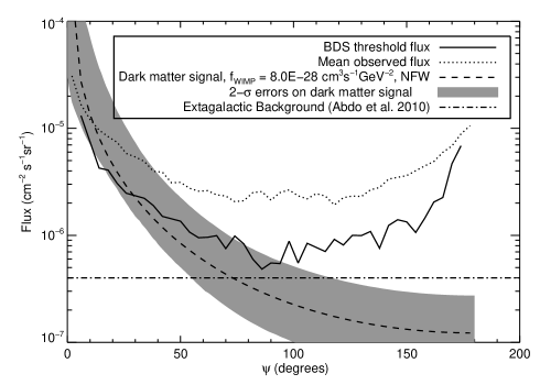
Figure 4: Plot of the upper limit flux, $F^{\rm{UL}}_{i}$, in the $i$th ring (solid line) determined using the BDS test as a function of the angle from the Galactic Center, $\psi$, at which the ring lies. This threshold flux represents the maximum flux possible for any i.i.d. component in that ring. The dotted curve shows the mean flux in the $i$th ring for comparison. The dashed curve represents the expected signal from the smooth dark matter in our galaxy assuming $f_{\mathrm{WIMP}}=8\times 10^{-28}\textrm{cm}^{3}\textrm{s}^{-1}\textrm{GeV}^{-2}$ and a canonical halo model; the shaded region represents the errors on the expected dark matter signal when uncertainties in the halo properties are taken into account. The dash-dotted line corresponds to the value of the extragalactic flux determined by the analysis of Ref. Abdo et al. (2010b). We have restricted the data in the plot to $1\,{\rm GeV}\,<E<100\,{\rm GeV}\,$ and have used 45 rings of equal angular width in $\psi$ across the sky.

As a consistency check on our results, we compare the minimum threshold flux in Fig. 4 (which occurs near $\psi=90^{\circ}$ as expected since this high-latitude region is least contaminated by the Galaxy) to the value of the extragalactic  $\gamma$-ray background determined by the analysis of the Fermi Collaboration in Ref. Abdo et al. (2010b) (see the dash-dotted line in Fig. 4). Since any isotropic, smooth background is necessarily i.i.d. we expect our minimum threshold flux to be at least as large as the measured isotropic background. We do not expect the minimum threshold flux to be much larger than the isotropic background, however, because the isotropic background dominates at $\psi\approx 90^{\circ}$. As expected, our minimum threshold flux of roughly $5\times 10^{-7}\rm{cm}^{-2}\rm{s}^{-1}\rm{sr}^{-1}$ is slightly larger than the value of $\sim 4\times 10^{-7}\rm{cm}^{-2}\rm{s}^{-1}\rm{sr}^{-1}$ obtained by Ref. Abdo et al. (2010b) for the extragalactic  $\gamma$-ray background flux over the same energy range ($1\,{\rm GeV}\,<E<100\,{\rm GeV}\,$).

Also shown in Fig. 4 is the flux predicted from the smooth dark matter component for a particular particle mass and cross section ($f_{\rm{WIMP}}$ is defined in the next section) and a smooth Navarro-Frenk-White (NFW) Navarro et al. (1996) distribution with canonical values for the total halo mass and concentration. The shaded region (described in the next section) reflects the uncertainties in the dark matter distribution. Roughly, then, these values of the mass and cross section are ruled out by the Ring Analysis. In the next section, we will project this constraint on to the mass–cross section plane and propagate the uncertainties in the dark matter distribution to this plane. Here, we note that the most stringent limit comes from the ring with $\psi=15^{\circ}$; this model-independent limit is:

$$F_{\rm{i.i.d.}}(\psi=15^{\circ})\leq 4.5\times 10^{-6}\rm{cm}^{-2}\rm{s}^{-1}\rm{sr}^{-1}.$$ (1)

The fact that this analysis identifies the annulus at $\psi=15^{\circ}$ as the most constraining is consistent with the arguments of Ref. Stoehr et al. (2003).

Fig. 4 also shows the mean flux in each ring. The mean flux is always larger than the i.i.d. upper limit; in the most constraining ring at $\psi=15^{\circ}$, the i.i.d. limit is a factor of 2 below the mean flux. This factor of two illustrates the power of the i.i.d. analysis: the limit obtained from the mean in the ring is contaminated by flux near the Galactic plane, contamination that is removed by the Ring Analysis introduced here.

The main advantage of the Ring Analysis is that it makes no assumptions about the source or properties of the backgrounds to the dark matter signal. This is a significant advantage because uncertainties in backgrounds are the main limitation for constraining dark matter with  $\gamma$-ray observations. We have assumed only that the signal in each pixel is drawn from a distribution that is invariant under rotations around the Galactic Center. Of course, the cost of assuming little is that the limit that can be placed using this technique is comparatively weak. For instance, since any isotropic backgrounds present in the data will also meet these assumptions, their presence will make our determined limit worse. Furthermore, we note that this technique is not well suited for actually detecting dark matter, but rather should be viewed as a way of placing upper limits on the dark matter signal.

IV Constraints on Dark Matter

IV.1 The Dark Matter Signal

The Milky Way is believed to exist within a roughly spherical halo of dark matter Zaritsky (1999). Consequently, the annihilation signal from galactic dark matter is expected to have azimuthal symmetry around the line connecting us to the Galactic Center. The dark matter constituting the halo is in turn thought to exist in two forms: a smooth component and a clumped component termed subhalos Diemand et al. (2007). Almost by definition, a smooth dark matter component will have an annihilation signal for which variations from the mean are uncorrelated. Therefore, the annihilation signal from smooth dark matter is a perfect candidate for the Ring Analysis developed in the previous section. Here we ignore potential signals from annihilations occurring in subhalos, as well as a possible cosmological signal from dark matter annihilations. Therefore, the constraint – on only the smooth Galactic component – is conservative.

In order to turn the flux limit derived by the Ring Analysis into constraints on the dark matter particle properties, we must develop a model for the expected annihilation flux from smooth Galactic dark matter. The observed flux of photons due to such annihilations along a given line of sight is

$$F(\psi)=\frac{f_{\rm{WIMP}}J(\psi)}{4\pi}$$ (2)

where the first factor on the right

$$f_{\rm{WIMP}}\equiv\frac{N_{\gamma}\langle\sigma v\rangle}{M_{\chi}^{2}}$$ (3)

depends on the particle physics properties of the dark matter: mass $M_{\chi}$, velocity-weighted annihilation cross section $\langle\sigma v\rangle$, and photon counts per annihilation

$$N_{\gamma}=\int_{E_{min}}^{E_{max}}\frac{dN}{dE}dE$$ (4)

within some desired band $E_{min}<E<E_{max}$. The second factor in Eq. (2)

$$J(\psi)\equiv\int dld\Omega\rho^{2}(l,\psi)$$ (5)

depends on the distribution of the dark matter halo, with $\rho(l,\psi)$ the smooth dark matter density at line of sight distance $l$ and zenith angle $\psi$. We have assumed that $\rho$ is spherically symmetric about the Galactic Center so that the observed flux can be written as a function of $\psi$ only but will revisit this assumption later. A given profile and therefore a value of $J$ translates the constraints on the i.i.d. flux in the previous section into a constraint on $f_{\rm{WIMP}}$ .

A canonical $J$ emerges from assuming an NFW profile with a scale radius of 20 kpc and local dark matter density of $\rho_{0}=0.43\,{\rm GeV}\,\rm{cm}^{-3}$. This leads to the $J(\psi)$ depicted as the dashed line in Fig. 4 for the given value of $f_{\rm{WIMP}}$ .

IV.2 Uncertainties in the Dark Matter Profile

The dark matter profile is not constrained very tightly by observations, and this uncertainty propagates to the constraints on the particle physics properties. We address this in two ways here, the first applies to all constraints on the smooth halo and the second is specific to our assumption that the dark matter distribution is spherical.

To allow for freedom in the dark matter profile, we piggy-back on the analysis of Ref. Widrow et al. (2008). They used nine sets of observational data to constrain the dark matter profile in our Galaxy. They assumed a density of the form

$$\rho(r)=\frac{2^{2-\gamma}\sigma_{h}^{2}}{4\pi a_{h}^{2}G}\frac{1}{(r/a_{h})(1+r/a_{h})^{3-\gamma}}$$ (6)

where $r$ is the distance from the Galactic Center, $a_{h}$ is the scale radius of the dark matter halo, $\sigma_{h}$ is a scale velocity, and $\gamma$ is a parameter which effects the behavior of the central density cusp, with $\gamma=1$ corresponding to the usual NFW form. A given set of these free parameters translates into a set of values for $J(\psi)$ assuming the distance between the Earth and the Galactic Center to be 8.5 kpc.

Figure 5: Histogram of values of $J(\psi)=\int dl\rho^{2}(\ell,\psi)$ corresponding to models in the MCMC chains provided by Widrow et al. (2008). We show the histograms for $\psi=10^{\circ}$ and $\psi=15^{\circ}$ since these angles provide the strongest constraint on dark matter annihilations. The broad histogram for $\psi=5^{\circ}$ illustrates the well-known statement that the uncertainty in the flux increases towards the Galactic Center.

The allowed values of the three profile parameters (and therefore $J(\psi)$) are contained in Monte Carlo Markov Chains run in Ref. Widrow et al. (2008). They have kindly provided us with those chains, and Fig. 5 projects these on to $J(\psi)$ for three different values of $\psi$. It is clear from this figure that the width of the distributions increases rapidly with decreasing $\psi$.

The widths of the distributions show in Fig. 5 can be propagated directly into error bars on the expected signal for dark matter in Fig. 4. The shaded region in Fig. 4 represents the 95% confidence interval for the allowed dark matter signal for a particular choice of $f_{\rm{WIMP}}$ . The value we have chosen for $f_{\rm{WIMP}}$ is illustrative in the sense that it is roughly the lowest value that is excluded by the Ring Analysis limit.

Our analysis so far has assumed that the signal from the smooth component of the dark matter is spherically distributed around the Galactic Center. In fact, the true shape of the Milky Way’s dark matter halo may be triaxial Law et al. (2009). If this is the case, then the dark matter signal is not uniform in rings of constant $\psi$ on the sky; instead, the signal in such a ring will be an oscillating function of the azimuth angle $\phi$ (the thick curves in Fig. 6). As a result, the total signal in a given ring will no longer be i.i.d. (i.e., it is not identical). However, there will still be some component of the signal that is i.i.d.; the flux of this component is given by the minimum flux of the dark matter signal in the ring (the thin horizontal lines in Fig. 6). Since the triaxiality of the halo effectively decreases the magnitude of the i.i.d. signal, the stated lower bound is too aggressive. It is therefore important to quantify how the triaxiality of the halo effects the level of the i.i.d. signal.

In order to estimate the magnitude of this effect, we calculate

$$J(\psi,\phi)\equiv\int dld\Omega\rho^{2}(l,\psi,\phi)$$ (7)

along different lines of sight in model triaxial galaxies. $J(\psi,\phi)$ is the analogue of $J(\psi)$ for a dark matter halo that is not assumed to be spherically symmetric. Observations in the Milky Way by Ref. Law et al. (2009) and simulations of disk galaxies by Ref. Bailin et al. (2005) suggest that one of the axes of the inner halo (which is also the region that dominates our exclusion limit) is aligned with the rotation axis of the galactic disk. Following the results of Ref. Law et al. (2009), we assume that the minor and major axes of the halo lie in the galactic plane; we find, however, that this choice of alignment does not have a significant impact on our results. We assume a density profile of the form Eq. 6 with the replacement

$$r^{2}=(x/c)^{2}+(y/a)^{2}+(z/b)^{2}$$ (8)

where the $x$, $y$ and $z$ axis are aligned with the minor, major and intermediate axes of the halo respectively. Strictly speaking, Refs. Jing and Suto (2002); Allgood et al. (2006) have found that the axis ratios $a/b$ and $b/c$ do not remain constant throughout the halo; rather, they decrease slightly (i.e. the ellipsoid becomes more elongated) towards the center of the halo. However, since our exclusion limit is dominated by a small range of distances from the Galactic Center we feel justified in approximating the halo by ellipsoids with constant axis ratios and alignments throughout the galaxy as per Eq. 8.

Fig. 6 shows $J(\psi=10^{\circ},\phi)$ along different lines of sight in model galaxies with several values of the axis ratios (thick lines). In generating this plot we have used $\sigma_{h}=270\textrm{km/s}$, $a_{h}=5.9\textrm{ kpc}$ and $\gamma=0.028$; in a spherical halo these values yield a J($\psi=10^{\circ}$) which is at the fifth percentile of all those calculated from the Markov chains of Ref. Widrow et al. (2008). Since the uncertainty in our exclusion limit is dominated by uncertainty in the halo model, this parameter choice is therefore appropriate for our $95\%$ exclusion limit on the dark matter properties. We plot only those lines of sight with $\psi=10^{\circ}$ because this is the angular range relevant to our exclusion limit. All of the curves have been normalized so that they have the same mean as the corresponding curve for a spherical halo; since the total amount of dark matter in the inner halo is strongly constrained (by measurements of galactic rotation curves, for instance), we expect this choice of normalization to be reasonably accurate.

To proceed further, we need to know the axis ratios of the isodensity surfaces throughout the Milky Way halo. Ref. Law et al. (2009) determined values for the axis ratios of some of the isovelocity surfaces in the Milky Way. While these values could in principle be converted to axis ratios for the isodensity surfaces given a density model, the large uncertainties associated with these measurements lead us to take a hopefully more robust approach. Using numerical simulations, Refs. Jing and Suto (2002); Allgood et al. (2006) have determined probability distributions for the axis ratios of dark matter halos. We run Monte Carlo simulations based on these results in order to quantify the extent of the variation in the dark matter signal due to triaxiality.

We calculate $J(\psi,\phi)$ for halos with axis ratios drawn from the probability distributions of Eqs. 17 and 18 in Ref. Jing and Suto (2002). We adjust these distributions slightly to account for the fact that they are calculated at a distance from the Galactic Center, $r_{2500}$, given by $\rho(r_{2500})/\rho_{\mathrm{crit}}=2500$ (note that $r_{2500}$ is defined in terms of the local halo density and not the mean interior density) while we are interested in the distributions much closer to the Galactic Center. Using Eqs. 6 and 7 of Ref. Jing and Suto (2002) we scale the axis ratios so that they correspond to a distance of $\sim 1.5\textrm{ kpc}$ from the Galactic Center, roughly the innermost distance that effects our constraint. This corresponds to decreasing $a/c$ and $b/c$ by roughly 30% and 10% respectively. The resultant distributions are roughly consistent with the results of Ref. Allgood et al. (2006). Finally, we assume that the line connecting the sun to the Galactic Center lies in the plane of the minor and major axes of the halo but with a random orientation in that plane.

Figure 6: The value of $J(\psi=10^{\circ},\phi)$ along different lines of sight for three model triaxial galaxies (thick lines). The minor, intermediate and major axes are labelled by $a$, $b$ and $c$ respectively. Also plotted are the corresponding levels of the i.i.d. component of the signal (thin lines). Following the results of Ref. Law et al. (2009) we have assumed that the minor and major axes of the halo lie in the galactic plane and that the line connecting the sun to the Galactic Center is offset from the minor axis of the halo by $15^{\circ}$.

Fig. 6 shows the flux as a function of azimuthal angle $\phi$ in a given ring for three different sets of $(a,b,c)$. The key take-away from these plots is the difference between the mean flux (i.e. the mean value of $J(\psi=10^{\circ},\phi)$ for the thick curves in Fig. 6) and the minimum flux (i.e. the thin curves in Fig. 6) in the ring. This difference is the amount by which we have been implicitly overestimating the i.i.d. signal. Dividing the difference by the mean flux then provides an estimate of the relative over-estimation, the amount by which we should loosen the i.i.d. constraint. Fig. 7 shows the distribution of this fractional difference (also at $\psi=10^{\circ}$) for 10000 Monte Carlo realizations of the halo axis ratios drawn from the probability distributions of Ref. Jing and Suto (2002). It is clear from this figure that error introduced by assuming a spherical halo is typically no more than $25\%$. Since the uncertainty introduced into our exclusion limit by the uncertainties in $\sigma_{h}$, $a_{h}$ and $\gamma$ is much greater than this, and since the degree of triaxiality in our own halo is not very well constrained, we choose to ignore this source of uncertainty in our exclusion plots.

Figure 7: Distribution of the percentage variation (mean to minimum) of the signal from smooth dark matter at $\psi=10^{\circ}$ in 10000 realizations of our Monte Carlo modeling of triaxial halos. Axis ratios have been drawn from the probability distributions of Ref. Jing and Suto (2002) (scaled according to the prescription described in the text). The line connecting the sun to the Galactic Center is assumed to lie in the plane of the minor and major axes of the halo, but with a random orientation in that plane.

We conclude this section by mentioning that the presence of baryons may have a non-negligible impact on the shape of the dark matter halo, particularly in the innermost region Springel et al. (2004). The effects of baryons have not been included in the simulations of Ref. Jing and Suto (2002) nor Ref. Allgood et al. (2006). While there may be a disturbance due to baryons near disk, the effect of such a disturbance on our exclusion limit is likely negligible since the limit is dominated by the region away from the disk where the backgrounds are lowest.

IV.3 Constraints on Dark Matter

The previous discussion has constrained $f_{\rm{WIMP}}$ over the energy range 1 GeV to 100 GeV . We find that our final constraint over this energy range is

$$f_{\rm{WIMP}}\leq 5.8\times 10^{-28}{\rm cm}^{3}\,{\rm s}^{-1}\,{\rm GeV}^{-2}$$ (9)

In order to turn the limits on $f_{\rm{WIMP}}$ into constraints on the dark matter particle properties we must assume an annihilation channel for the dark matter so that $N_{\gamma}$ (Eq. 4) can be calculated. The constraint on $f_{\rm{WIMP}}$ and the value of $N_{\gamma}$ can then be transformed into a constraint in the $M_{\chi}$-$\langle\sigma v\rangle$ parameter space using Eq. 3.

The choice of the energy range that we impose on our analysis can have a significant impact on the constraints that we place in the $M_{\chi}$-$\langle\sigma v\rangle$ plane. For $E\ll M_{\chi}$ the annihilation photon spectrum is relatively flat compared to that of the backgrounds, so increasing $E_{\mathrm{min}}$ in this regime effectively increases the size of the signal relative to the total flux, thereby improving the constraint on the dark matter properties. As $E$ approaches $M_{\chi}$, the spectrum of annihilation photons falls off very quickly so increasing $E_{\mathrm{min}}$ in this regime causes the constraint to become very weak. We expect, then, that the optimal constraint on the dark matter comes from choosing $E_{\mathrm{min}}$ to be some fixed fraction of $M_{\chi}$. Rather than enforcing the optimal $E_{\mathrm{min}}$ for each $M_{\chi}$ exactly (which would require dividing the data into many more energy bins than the 29 that we employ), we allow $E_{\mathrm{min}}$ to vary freely for each $M_{\chi}$ that we consider. We then choose the value of $E_{\mathrm{min}}$ that maximizes our constraint on the dark matter. Random fluctuations in the strength of the constraint induced by varying $E_{\mathrm{min}}$ are small, so choosing $E_{\mathrm{min}}$ to maximize the constraint does not decrease the statistical significance of our result. Varying $E_{\mathrm{min}}$ is our one minimal use of the energy information for the photons; by making our analysis essentially independent of detailed spectral information we make our constraints more robust.

Fig. 8 shows how the constraints that we place on $f_{\rm{WIMP}}$ in different energy bins with the Ring Analysis are translated into constraints in the $M_{\chi}$-$\langle\sigma v\rangle$ plane for different assumed annihilation channels (each of which correspond to a different $N_{\gamma}$). We consider two possible annihilation channels: $\chi\chi\rightarrow b\bar{b}$ and $\chi\chi\rightarrow\tau\bar{\tau}$, where $\chi$ is a neutralino. $N_{\gamma}$ is calculated for these different channels over a mass range of 10 GeV to 10 TeV using the DarkSUSY package Gondolo et al. (2004). Since our technique places a limit on $f_{\rm{WIMP}}=N_{\gamma}\langle\sigma v\rangle/M_{\chi}^{2}$ we expect the limit on $\langle\sigma v\rangle$ to go roughly as $M_{\chi}^{2}$. The flattening of the limit at low mass is due to a decrease in $N_{\gamma}$ as more and more annihilation photons fall outside of the energy limits of our analysis.

The dashed curves in Fig. 8 show what the limit would be if the dark matter profile, as quantified by $J(\psi)$, produced the mean annihilation signal, and there was no uncertainty in the profile. The uncertainty in dark matter profile then loosens the constraint on the annihilation cross section by more than a factor of 2.

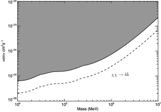
Figure 8: Exclusion plots in the $\langle\sigma v\rangle$-$M_{\chi}$ plane generated by the Ring Analysis for different annihilation channels of the dark matter. The solid region represent the 95% exclusion range with respect to the uncertainties in the properties of the smooth halo. The dashed line represents the boundary of the excluded region when the mean value of $J(\psi)$ from the Monte Carlo chains of Ref. Widrow et al. (2008) is used to calculate the expected dark matter signal. The left panel shows the exclusion limit for neutralinos, $\chi$, that annihilated to $b\bar{b}$; the right panel corresponds to neutralinos annihilating to $\tau\bar{\tau}$.

The limits presented in Fig. 8 are comparable to the corresponding plots from Ref. Zaharijas et al. (2010), which also considers the annihilation signal from the smooth galactic dark matter component, but which makes a stronger set of assumptions about the signal and backgrounds. Our limits are complementary in the sense that they are almost entirely independent of any assumptions about the diffuse  $\gamma$-ray background. We also find that our constraints are comparable to those obtained from an analysis of extragalactic dark matter annihilations by Ref. Abdo et al. (2010a). As evidenced in Fig. 5 of that work, the constraints derived from extragalactic annihilations are subject to very large uncertainties in the magnitude of the dark matter signal. While uncertainties in the signal from smooth galactic dark matter are also important, they are not nearly as large. Finally, our limits are also comparable to (and competitive with) those derived from an analysis of the annihilation signal from dwarf spheroidal galaxies by Ref. Abdo et al. (2010c).

V Summary

We have developed a technique for constraining the presence of a smooth, azimuthally symmetric signal on the sky. We showed with Monte Carlo simulations that the technique is robust (i.e. the limits derived from the technique are never below the mean signal flux). By applying the technique to data from the Fermi Gamma-Ray Space Telescope we derived a constraint (Eq. (1)) on the presence of any smooth  $\gamma$-ray signal that is symmetric with respect to rotations about the axis connecting us to the Galactic Center. When combined with a model for the signal due to annihilations of the smooth dark matter component in our galaxy, these limits allow us to place constraints on the dark matter particle mass and cross section. While our limits are slightly weaker than other recent results, they have the advantage of making essentially no assumptions about the backgrounds to the dark matter signal. This is a significant advantage because the uncertainties in models of  $\gamma$-ray backgrounds are large and often unknown.

There are several ways these limits can be improved. Tighter constraints on the dark matter profile would reduce the uncertainty in $J(\psi)$, which currently degrades the ultimate limit by more than a factor of 2. Including other sources of signal, in particular the contribution from extra-galactic halos, would improve the signal, but in most models, this contribution is smaller than that from the Galactic halo. A deeper understanding of the backgrounds could also be used in conjunction with this method to push the limits down further.

Acknowledgments We are very grateful to Larry Widrow for providing us with the chains from Ref. Widrow et al. (2008) and to Andrey Kravtsov for his guidance on the properties of the Galactic halo. This work has been supported by the US Department of Energy, including grant DE-FG02-95ER40896, and by National Science Foundation Grant AST-0908072.

References

- Jarosik et al. (2010) N. Jarosik, C. L. Bennett, J. Dunkley, B. Gold, M. R. Greason, M. Halpern, R. S. Hill, G. Hinshaw, A. Kogut, E. Komatsu, et al., ArXiv e-prints (2010), eprint 1001.4744.
- Bergstrom et al. (2010) L. Bergstrom, T. Bringmann, and J. Edsjo, ArXiv e-prints (2010), eprint 1011.4514.
- Landsman and Icecube Collaboration (2007) H. Landsman and Icecube Collaboration, in The Identification of Dark Matter, edited by M. Axenides, G. Fanourakis, & J. Vergados (2007), pp. 450–+, eprint arXiv:astro-ph/0612239.
- Horns and H.E.S.S. collaboration (2008) D. Horns and H.E.S.S. collaboration, Advances in Space Research 41, 2024 (2008), eprint arXiv:astro-ph/0702373.
- Holder et al. (2006) J. Holder, R. W. Atkins, H. M. Badran, G. Blaylock, S. M. Bradbury, J. H. Buckley, K. L. Byrum, D. A. Carter-Lewis, O. Celik, Y. C. K. Chow, et al., Astroparticle Physics 25, 391 (2006), eprint arXiv:astro-ph/0604119.
- Picozza et al. (2007) P. Picozza, A. M. Galper, G. Castellini, O. Adriani, F. Altamura, M. Ambriola, G. C. Barbarino, A. Basili, G. A. Bazilevskaja, R. Bencardino, et al., Astroparticle Physics 27, 296 (2007), eprint arXiv:astro-ph/0608697.
- Atwood et al. (2009) W. B. Atwood, A. A. Abdo, M. Ackermann, W. Althouse, B. Anderson, M. Axelsson, L. Baldini, J. Ballet, D. L. Band, G. Barbiellini, et al., Astrophys. J. 697, 1071 (2009), eprint 0902.1089.
- Abdo et al. (2010a) A. A. Abdo, M. Ackermann, M. Ajello, L. Baldini, J. Ballet, G. Barbiellini, D. Bastieri, K. Bechtol, R. Bellazzini, B. Berenji, et al., JCAP 4, 14 (2010a).
- Zaharijas et al. (2010) G. Zaharijas, A. Cuoco, Z. Yang, and J. Conrad, ArXiv e-prints (2010), eprint 1012.0588.
- Hooper and Goodenough (2010) D. Hooper and L. Goodenough, arXiv, 1010.2752 (2010).
- Lee et al. (2009) S. K. Lee, S. Ando, and M. Kamionkowski, ”JCAP” 7, 7 (2009), eprint 0810.1284.
- Dodelson et al. (2009) S. Dodelson, A. V. Belikov, D. Hooper, and P. Serpico, Phys. Rev. D80, 083504 (2009), eprint 0903.2829.
- Baxter et al. (2010) E. J. Baxter, S. Dodelson, S. M. Koushiappas, and L. E. Strigari, Phys. Rev. D82, 123511 (2010), eprint 1006.2399.
- Siegal-Gaskins and Pavlidou (2009) J. M. Siegal-Gaskins and V. Pavlidou, Phys. Rev. Lett. 102, 241301 (2009), eprint 0901.3776.
- Hensley et al. (2010) B. S. Hensley, J. M. Siegal-Gaskins, and V. Pavlidou, Astrophys. J. 723, 277 (2010), eprint 0912.1854.
- Abdo et al. (2010b) A. A. Abdo, M. Ackermann, M. Ajello, W. B. Atwood, L. Baldini, J. Ballet, G. Barbiellini, D. Bastieri, B. M. Baughman, K. Bechtol, et al., Physical Review Letters 104, 101101 (2010b), eprint 1002.3603.
- Ackermann et al. (2008) M. Ackermann, G. Jóhannesson, S. Digel, I. V. Moskalenko, T. Porter, O. Reimer, and A. Strong, in American Institute of Physics Conference Series, edited by F. A. Aharonian, W. Hofmann, & F. Rieger (2008), vol. 1085 of American Institute of Physics Conference Series, pp. 763–766.
- Brock et al. (1987) W. Brock, W. Dechert, and J. Scheinkman, SSRI Working Paper No. 8702. (1987).
- Cromwell (1994) J. Cromwell, Univariate tests for time series models (Sage Publications, Thousand Oaks, Calif, 1994), ISBN 080394991X.
- LeBaron (1997) B. LeBaron, Studies in Nonlinear Dynamics & Econometrics 2 (1997).
- Brock and Baek (1991) W. A. Brock and E. Baek, Review of Economic Studies 58, 697 (1991).
- Navarro et al. (1996) J. F. Navarro, C. S. Frenk, and S. D. M. White, Astrophys. J. 462, 563 (1996), eprint arXiv:astro-ph/9508025.
- Stoehr et al. (2003) F. Stoehr, S. D. M. White, V. Springel, G. Tormen, and N. Yoshida, Mon. Not. Roy. Astron. Soc. 345, 1313 (2003), eprint astro-ph/0307026.
- Zaritsky (1999) D. Zaritsky, in The Third Stromlo Symposium: The Galactic Halo, edited by B. K. Gibson, R. S. Axelrod, & M. E. Putman (1999), vol. 165 of Astronomical Society of the Pacific Conference Series, pp. 34–+, eprint arXiv:astro-ph/9810069.
- Diemand et al. (2007) J. Diemand, M. Kuhlen, and P. Madau, Astrophys. J. 657, 262 (2007), eprint arXiv:astro-ph/0611370.
- Widrow et al. (2008) L. M. Widrow, B. Pym, and J. Dubinski, Astrophys. J. 679, 1239 (2008), eprint 0801.3414.
- Law et al. (2009) D. R. Law, S. R. Majewski, and K. V. Johnston, Astrophys. J. Lett. 703, L67 (2009), eprint 0908.3187.
- Bailin et al. (2005) J. Bailin, D. Kawata, B. K. Gibson, M. Steinmetz, J. F. Navarro, C. B. Brook, S. P. D. Gill, R. A. Ibata, A. Knebe, G. F. Lewis, et al., ApJL 627, L17 (2005), eprint arXiv:astro-ph/0505523.
- Jing and Suto (2002) Y. P. Jing and Y. Suto, Astrophys. J. 574, 538 (2002), eprint arXiv:astro-ph/0202064.
- Allgood et al. (2006) B. Allgood, R. A. Flores, J. R. Primack, A. V. Kravtsov, R. H. Wechsler, A. Faltenbacher, and J. S. Bullock, MNRAS 367, 1781 (2006), eprint arXiv:astro-ph/0508497.
- Springel et al. (2004) V. Springel, S. D. M. White, and L. Hernquist, in Dark Matter in Galaxies, edited by S. Ryder, D. Pisano, M. Walker, & K. Freeman (2004), vol. 220 of IAU Symposium, pp. 421–+.
- Gondolo et al. (2004) P. Gondolo, J. Edsjö, P. Ullio, L. Bergström, M. Schelke, and E. A. Baltz, JCAP 7, 8 (2004), eprint arXiv:astro-ph/0406204.
- Abdo et al. (2010c) A. A. Abdo, M. Ackermann, M. Ajello, W. B. Atwood, L. Baldini, J. Ballet, G. Barbiellini, D. Bastieri, K. Bechtol, R. Bellazzini, et al., Astrophys. J. 712, 147 (2010c), eprint 1001.4531.