Stability of Matter-Antimatter Molecules

Abstract

We examine the stability of matter-antimatter molecules by reducing the four-body problem into a simpler two-body problem with residual interactions. We find that matter-antimatter molecules with constituents $(m_{1}^{+},m_{2}^{-},{\bar{m}}_{2}^{+},{\bar{m}_{1}}^{-})$ possess bound states if their constituent mass ratio $m_{1}/m_{2}$ is greater than about 4. This stability condition suggests that the binding of matter-antimatter molecules is a rather common phenomenon. We evaluate the binding energies and eigenstates of matter-antimatter molecules $(\mu^{+}e^{-})$-$(e^{+}\mu^{-})$, $(\pi^{+}e^{-})$-$(e^{+}\pi^{-})$, $(K^{+}e^{-})$-$(e^{+}K^{-})$, $(pe^{-})$-$(e^{+}\bar{p})$, $(p\mu^{-})$-$(\mu^{+}{\bar{p}})$, and $(K^{+}\mu^{-})$-$(\mu^{+}K^{-})$, which satisfy the stability condition. We estimate the molecular annihilation lifetimes in their $s$ states.

I Introduction

The study of the stability and the properties of matter-antimatter molecules has a long history, starting with the pioneering work of Wheeler who suggested in 1946 that $(e^{+}e^{-})$ might be bound with its antimatter partner to form a matter-antimatter molecule Whe46 . Since then, the problem has been examined theoretically by many workers Hyl47 ; Mor73 ; Ho83 ; Gri89 ; Nus93 ; Koz93 ; Zyg04 ; Kolos ; Armour ; Froelich ; Jon01 ; Strasburger ; Labzowsky ; Sharipov (for a review and other references see Cha01 ). Wheeler went on to explore the properties of an assembly of $(e^{+}e^{-})^{n}$ atoms and molecules if they were made, and he outlined the phase boundaries in temperature and pressure separating various phases of $(e^{+}e^{-})$ atoms and $(e^{+}e^{-})$-$(e^{-}e^{+})$ molecules in their gaseous, liquid, super-fluid, crystal, and metallic states Whe88 . However, the experimental detection of matter-antimatter molecules is difficult, and the $(e^{+}e^{-})$-$(e^{-}e^{+})$ molecule was successfully detected only recently, as late as 2007 Cas07 .

In spite of extensive past investigations, our knowledge of matter-antimatter molecules remains rather incomplete, being limited to $(e^{+})^{m}(e^{-})^{n}$ and some aspects of $(pe^{-})$-$(e^{+}{\bar{p}})$. There are however stable and meta-stable charged particles and antiparticles, such as $e^{\pm}$, $p\bar{p}$, $\mu^{\pm}$, $\pi^{\pm}$, $K^{\pm}$, $\tau^{\pm}$, etc. The conditions for the molecular binding of four-body particle-antiparticle complexes containing these charged constituents are not known, nor are their annihilation lifetimes, if these matter-antimatter molecules turn out to be bound.

With the advent of the Relativistic Heavy-Ion Collider at Brookhaven and the Large hadron Collider at CERN, a large number of charged particles and antiparticles are produced in high-energy $pp$ and heavy-ion collisions. The production of matter and antimatter particles in close space-time proximity raises the interesting question whether chance encounters of some of the produced charged particles and antiparticles may lead to the formation of matter-antimatter molecules as debris of the collision. The detection of matter-antimatter molecules in high-energy nuclear collisions will need to overcome the difficulty of large combinatorial background noises that may be present. In another related area, recent production and trapping of cold antihydrogen Amoretti ; Gabrielse ; And10 provide the possibility of bringing matter and antimatter atoms close together. Furthermore, electron-positron colliders with fine energy resolutions may be used to produce stable matter-antimatter molecules as resonances with finite widths, when the colliding $e^{+}$ and $e^{-}$ combination has the same quantum number as the matter-antimatter molecules.

The detection of new matter-antimatter molecules is however a difficult task, as evidenced by the long span of time between the proposal and the observation of the $(e^{+}e^{-})$-$(e^{-}e^{+})$ molecule. Additional instrumentation and experimental apparatus may be needed. It is nonetheless an interesting theoretical question to investigate systematically the general factors affecting the stability of matter-antimatter molecules, whether any of these matter-antimatter molecules may be bound, and if they are bound, what are their binding energies, annihilation lifetimes, and other characteristics. Answers to these questions will help us assess whether it may ever be feasible to detect them experimentally in the future.

Following Wheeler Whe46 , we shall use the term “atom” to represent a two-body bound state of a positive and a negative charged pair that can form a building block, out of which more complex “molecules” can be constructed. In the present work, we shall limit our attention to molecules in which the four constituents $\{m_{1}$, $m_{2}$, $m_{3}$, $m_{4}\}$ consist of two charge conjugate pairs, with $m_{3}$ the charge conjugate of $m_{2}$, and $m_{4}$ the charge conjugate of $m_{1}$. We shall arrange and order the constituents according to their masses such that $m_{1}$$>$$m_{2}$, and the charges of $m_{1}$ and $m_{2}$ be $+e$ and $-e$ respectively. To make the problem simple, we shall consider molecules containing non-identical constituents $m_{1}$ and $m_{2}$ and their antiparticle counterparts, such that there are no identical particles among the constituents. Molecules with identical constituents require additional considerations on the symmetries of the wave function with respect to the exchange of the pair of identical particles, which are beyond the scope of the present investigation.

To study the structure of the molecules, we shall consider only Coulomb interactions between particles and neglect strong interactions, as the range of strong interactions is considerably smaller than the Bohr radius of the relevant particle-antiparticle system.

Previously, based on the method proposed for the study of molecular states in heavy quark mesons Won04 , we obtained the interatomic potential for the $H\bar{H}$ system Lee08 . We shall generalize our consideration to cases of constituent particles of various masses and types and shall quantize the four-body Hamiltonian to obtain molecular eigenstates of the four-body system. If molecular states are found, we shall determine their annihilation lifetimes and their spin dependencies, if any.

It is worth pointing out that the subject matter of molecular states appears not only in atomic and molecular physics, but also in nuclear physics and hadron spectroscopy. Wheeler’s 1937 article entitled “Molecular Viewpoints in Nuclear Structure” introduced molecular physics concepts such as resonating groups and alpha particle groups to nuclear physics Whe37 . Indeed, nucleus-nucleus molecular states have been observed previously in the collision of light nuclei near the Coulomb barrier Alm60 . Molecular states of heavy-quark mesons have been proposed in high-energy hadron spectroscopy Won04 ; Tor03 ; Clo04 ; Bra04 ; Swa04 to explain the narrow 3872 MeV state discovered by the Belle Collaboration Cho03 and other Collaborations Aco04 . The general stability condition established here for the Coulomb four-body problem for matter-antimatter molecules may have interesting implications or generalizations in other branches of physics.

This paper is organized as follows. In Section II, we review the families of states of the four-body matter-antimatter system so as to introduce the method of our investigation. In Section III, the mathematical details of our formulation are presented and the four-body problem is reduced to a simple two-body problem in terms of the interaction of two atoms with residual interactions. The interaction potential is found to consist of the sum of the direct potential $V_{\rm dir}$ and the polarization potential $V_{\rm pol}$. In Section IV, we show how to evaluate the interaction matrix elements. In Section V, we show the analytical result for the direct potential $V_{\rm dir}$. In Section VI, the polarization potential is evaluated for the virtual excitation to the complete set of bound and continuum atomic states. The results of the interaction potential for $(pe^{+})$-$(e^{+}{\bar{p}})$ are discussed in Section VII. The interaction potentials for other molecular systems are examined in Section VIII. In Section IX, we solve the Schrödinger equation for molecular motion and obtain the molecular eigenstates for different systems. We discuss the annihilation rates and lifetimes of the molecular states in Section X. Finally, Section XI gives some discussions and conclusions of the present work. Some of the details of the analytical results are presented in the Appendix.

II Families of four-particle states

The four constituent particles can be arranged in different ways leading to different types of states. There is the $A{\bar{A}}$ family of states of the type $A(m_{1}^{+}m_{2}^{-})$-${\bar{A}}({\bar{m}}_{2}^{+}{\bar{m}_{1}}^{-})$, in which $m_{1}^{+}$ and $m_{2}^{-}$ orbit around each other to form the $A_{\nu}(m_{1}^{+}m_{2}^{-})$ atom in the $\nu$ state, while ${\bar{m}}_{2}^{+}$ and ${\bar{m}}_{1}^{-}$ orbit around each other to form the ${\bar{A}}_{\nu^{\prime}}({\bar{m}}_{2}^{+}{\bar{m}}_{1}^{-})$ atom in the ${\nu^{\prime}}$ state. When $A_{\nu}$ and ${\bar{A}}_{\nu^{\prime}}$ are separated at large distances, their asymptotic state energy is

$$E_{A\bar{A}}(n_{\nu},n_{\nu^{\prime}})=-\alpha^{2}\frac{m_{1}m_{2}}{m_{1}+m_{2}}\left(\frac{1}{n_{\nu}^{2}}+\frac{1}{n_{\nu^{\prime}}^{2}}\right).$$ (1)

There is another $M\bar{M}$ family of states of the type $M(m_{1}^{+}{\bar{m}_{1}}^{-})$-${\bar{M}}({\bar{m}_{2}}^{+}m_{2}^{-})$, in which $m_{1}^{+}$ and ${\bar{m}}_{1}^{-}$ orbit around each other to form the $M_{\nu}(m_{1}^{+}{\bar{m}}_{1}^{-})$ atom in the $\nu$ state, while ${\bar{m}}_{2}^{+}$ and $m_{2}^{-}$ orbit around each other to form the ${\bar{M}}_{\nu^{\prime}}({\bar{m}}_{2}^{+}m_{2}^{-})$ atom in the $\nu^{\prime}$ state. Their asymptotic state energy is

$$E_{M{\bar{M}}}(n_{\nu},n_{\nu^{\prime}})=-\frac{1}{4}\alpha^{2}\left(\frac{m_{1}}{n_{\nu}^{2}}+\frac{m_{2}}{n_{\nu^{\prime}}^{2}}\right).$$ (2)

For the same values of $n_{\nu}=n_{\nu^{\prime}}$, the asymptotic state of the $M{\bar{M}}$ family lies lower in energy than the asymptotic state of the $A\bar{A}$ family, except when $m_{1}=m_{2}$ for which they are at the same level,

$$E_{M{\bar{M}}}(n_{\nu},n_{\nu})<E_{A\bar{A}}(n_{\nu},n_{\nu}) {\rm~{}~{}if~{}~{}} m_{1}\neq m_{2}$$

$${\rm and~{}~{}~{}}E_{M{\bar{M}}}(n_{\nu},n_{\nu})=E_{A\bar{A}}(n_{\nu},n_{\nu}) {\rm~{}~{}if~{}~{}} m_{1}=m_{2}.$$ (3)

On the other hand, by varying the principal quantum numbers, many of the asymptotic states of one family can lie close to the energy levels of the asymptotic states of the other family. Level crossing between states and the mixing of states of different families can occur when the atoms are brought in close proximity to each other.

There are two different methods to study molecular states. In the first method, one reduces the four-body problem into a simpler two-body problem. One breaks up the four-body Hamiltonian into the unperturbed Hamiltonians of two atoms, plus residual interactions and the kinetic energies of the atoms. The unperturbed Hamiltonians of the two atoms can be solved exactly. Using the atomic states as separable two-body basis, one constructs molecular states with the atoms as simple building blocks and quantize the four-particle Hamiltonian Won04 . The quantized eigenstate obtained in such a method may not necessarily contain all the correlations. They may also not necessarily be the lowest states of the four-body system. They however have the advantage that the center-of-mass motion of the composite atoms are properly treated and the formulation can be applied to systems with vastly different mass ratios $m_{1}/m_{2}$. They provide a clear and simple picture of the molecular structure. They also provide vital information on the condition of molecular stability and the values of molecular eigenenergies. The knowledge of the molecular eigenfunctions provides information on other properties of the molecular states and their annihilation lifetimes. Furthermore, these molecular states can form doorways for states of greater complexity with additional correlations. For example, one can multiply the four-body wave functions of a molecular state obtained in such a method (see Eq. (10) below) by a complete set of correlated wave functions for a particular pair of constituents, and diagonalize the four-body Hamiltonian with such a basis. The eigenstates obtained after such a diagonalization represent the splitting of the doorway state into finer molecular states containing additional correlations. As the method exhibits a clear molecular structure in terms of composite two-body objects, its asymptotic states illustrate how the molecule may be formed by the collision of the composite atoms. Finally, if one depicts the orbiting of one particle relative to another particle as a “dance pattern” with the topology of a ring, then the dance patterns of the different constituents and atoms in different families have distinctly different connectivities and topological structures. The transition of a state from one family to another family will involve the breaking of one type of dance pattern and re-establishing another type of dance pattern. It is reasonable to conjecture that their distinct topological structures may suppress the transition amplitude between families and may allow the atoms to retain some of their characteristics and stability in their dynamical motion and transitions.

There is an alternative second method to study the molecular states by taking the interaction potential to be the adiabatic potential obtained in a variational calculation for the lowest-energy state of the four particle complex in the Born-Oppenheimer potential, in which the positions of two heavy constituents are held fixed Zyg04 ; Kolos ; Armour ; Froelich ; Jon01 ; Strasburger ; Labzowsky ; Sharipov . It should be realized that such variational calculations have not yet been fully variational. By fixing the positions of the heavy constituents (the proton and antiproton in the case of the $(pe^{-}e^{+}{\bar{p}})$ complex), the trial wave functions of the heavy constituents have been constrained to be delta functions without variations. If the motion of the heavy constituents were allowed to vary in a fully variational calculation, the lowest energy state would be the one in which the heavy constituents would orbit around each other in their atomic orbitals, with binding energies proportional to their heavy masses. The variational calculations of the higher molecular states will need to insure the orthogonality of the state relative to lower lying ones. Furthermore, as the variational calculation searches for the state with the lowest energy, motion in the relative coordinates between the heavier masses corresponds to constraining a trajectory along a path with adiabatic transitions whenever a level crossing occurs. In a collective molecular motion, these level crossing may not necessarily be adiabatic Hil53 because the speed of the collective motion becomes large at small interatomic separations, and the transition matrix element between different families may be suppressed due to the difference in their topological structures. It is reasonable to suggest that while variational calculations may provide useful information on the four-particle complex, they should not be the only method to examine the molecular structure of the four-body system.

We shall use the first method to study the eigenstates of the four-body system and construct states built on the $A\bar{A}$ family. Accordingly, we break the four-body Hamiltonian into a part containing the unperturbed Hamiltonians of the $A$ and ${\bar{A}}$ atoms and another part containing the residual interactions and the kinetic energies of $A$ and $\bar{A}$. The quantization of the four-body Hamiltonian then gives the molecular states of interest, as in a previous study of molecular states in heavy mesons in hadron physics Won04 . Such a separation of the four-body Hamiltonian is justified because the composite $A$ and $\bar{A}$ atoms are neutral objects, and their residual interaction $V_{I}$ between the constituents of $A$ and $\bar{A}$ involve many cancellations. As a consequence, the non-diagonal matrix element for excitation arising from the residual interaction is relatively small in comparison with the difference between unperturbed state energies, and the perturbation expansion is expected to converge.

Molecular states can be constructed using composite objects of $A_{\nu}$ and ${\bar{A}}_{\nu^{\prime}}$ in various asymptotic $\nu$ and $\nu^{\prime}$ states. We shall be interested in molecular states in which the building block atoms $A_{0}$ and ${\bar{A}}_{0}$ are in their ground states at asymptotic separations. As the two ground state atoms approach each other, they will be excited and polarized and their virtual excitation will lead to an interaction potential between the atoms, from which the eigenstates of the molecule will be determined.

Molecular states constructed with excited $A_{\nu}$ and ${\bar{A}}_{\nu^{\prime}}$ atoms can be similarly considered in a simple generalization in the future. Such a possibility brings into focus the richness of states in the four-body system, as the molecular states will have different interatomic interactions, obey different stability conditions, and have different properties with regard to annihilation and production.

III The Four-body Problem in a Separable Two-Body Basis

In order to introduce relevant concepts and notations, we shall review the formulation of the four-body problem in terms of a simpler two-body problem Won04 . We choose the four-body coordinate system as shown in Fig. 1 and label constituents $m_{1}^{+}$, $m_{2}^{-}$, $m_{3}^{+}$, and $m_{4}^{-}$ as particles 1, 2, 3, and 4, respectively with $m_{1}$$>$$m_{2}$. The Hamiltonian for the four-particle system is

$$H=\sum_{j=1}^{4}\frac{\hbox{\boldmath${p}$}_{j}^{2}}{2m_{j}}+\sum_{j=1}^{4}\sum_{k>j}^{4}v_{jk}+\sum_{j=1}^{4}m_{j},$$ (4)

in which particle $j$ has a momentum $\hbox{\boldmath${p}$}_{j}$ and a rest mass $m_{j}$. The pairwise interaction $v_{jk}(\hbox{\boldmath${r}$}_{jk})$ between particle $j$ and particle $k$ depends on the relative coordinate between them, $\hbox{\boldmath${r}$}_{jk}=\hbox{\boldmath${r}$}_{j}-\hbox{\boldmath${r}$}_{k}.$

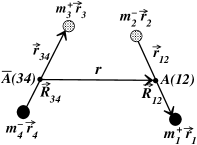
Figure 1: The coordinates of the $\{m_{1}^{+},m_{2}^{-},m_{3}^{+},m_{4}^{-}\}$ system.

We introduce the two-body total momentum ${\hbox{\boldmath${P}$}}_{jk}=\hbox{\boldmath${p}$}_{j}+\hbox{\boldmath${p}$}_{k},$ and the two-body relative momentum $\hbox{\boldmath${p}$}_{jk}=f_{k}\hbox{\boldmath${p}$}_{j}-f_{j}\hbox{\boldmath${p}$}_{k},$ where

$$f_{k} = \frac{m_{k}}{m_{jk}},$$

$$m_{jk} = m_{j}+m_{k}.$$ (5)

We choose to partition the four-body Hamiltonian in Eq. (4) into an unperturbed $h_{12}+h_{34}$ for atoms $A(12)$ and ${\bar{A}}(34)$, a residual interaction $V_{I}$, and the kinetic energies of $A$ and $\bar{A}$,

$$H=h_{12}+h_{34}+V_{I}+\frac{\hbox{\boldmath${P}$}_{12}^{2}}{2m_{12}}+\frac{\hbox{\boldmath${P}$}_{34}^{2}}{2m_{34}},$$ (6)

where

$$h_{jk}=\frac{\hbox{\boldmath${p}$}_{jk}^{2}}{2\mu_{jk}}+v_{jk}(\hbox{\boldmath${r}$}_{j}-\hbox{\boldmath${r}$}_{k})+m_{jk}{\rm~{}~{}~{}~{}for~{}~{}}\{jk\}=\{12\}{\rm~{}and~{}}\{34\},$$ (7)

and

$$V_{I}=v_{14}(\hbox{\boldmath${r}$}_{14})+v_{13}(\hbox{\boldmath${r}$}_{13})+v_{23}(\hbox{\boldmath${r}$}_{23})+v_{24}(\hbox{\boldmath${r}$}_{24}).$$ (8)

The eigenvalues of the unperturbed two-body Hamiltonians $h_{12}$ and $h_{34}$ can be solved separately to obtain the bound state wave functions and masses $M_{jk}(\nu)$ of atoms $A$ and ${\bar{A}}$,

$$h_{jk}|(jk)_{\nu}\rangle=[\epsilon_{jk}(\nu)+m_{jk}]|(jk)_{\nu}\rangle=M_{jk}(\nu)|(jk)_{\nu}\rangle.$$ (9)

When we include $V_{I}$ as a perturbation, the eigenfunction of ${H}$ becomes Lan58

$$\Psi (\hbox{\boldmath${r}$},\hbox{\boldmath${r}$}_{12},\hbox{\boldmath${r}$}_{34})=\psi(\hbox{\boldmath${r}$})\Biggl{\{}|A_{0}{\bar{A}}_{0}\rangle-{\sum_{\lambda,\lambda^{\prime}}}^{\prime}\frac{|A_{\lambda}{\bar{A}}_{\lambda^{\prime}}\rangle\langle A_{\lambda}{\bar{A}}_{\lambda^{\prime}}|V_{I}|A_{0}{\bar{A}}_{0}\rangle}{\epsilon_{A}({\lambda})+\epsilon_{\bar{A}}({\lambda^{\prime}})-\epsilon_{A}(0)-\epsilon_{\bar{A}}(0)}\Biggr{\}},~{}~{}~{}~{}~{}$$ (10)

where $\hbox{\boldmath${r}$}=\hbox{\boldmath${R}$}_{12}-\hbox{\boldmath${R}$}_{34}$ is the interatomic separation (see Fig. 1), $\hbox{\boldmath${R}$}_{jk}=f_{j}~{}\hbox{\boldmath${r}$}_{j}+f_{k}~{}\hbox{\boldmath${r}$}_{k}$ is the center-of-mass coordinate of $m_{j}$ and $m_{k}$, and $\sum_{\lambda\lambda^{\prime}}^{\prime}$ indicates that the sum is over a complete set of atomic states $|A_{\lambda}{\bar{A}}_{\lambda^{\prime}}\rangle$, including both bound and continuum states, except $|A_{0}{\bar{A}}_{0}\rangle$. The eigenvalue equation for the four-body system with eigenenergy $\epsilon$ is

$$H\Psi(\hbox{\boldmath${r}$},\hbox{\boldmath${r}$}_{12},\hbox{\boldmath${r}$}_{34})=[M_{12}(0)+M_{34}(0)+\epsilon]\Psi(\hbox{\boldmath${r}$},\hbox{\boldmath${r}$}_{12},\hbox{\boldmath${r}$}_{34}).$$ (11)

Working in the center-of-mass frame and taking the scalar product of the above equation with $|A_{0}{\bar{A}}_{0}\rangle$, the eigenvalue equation for the four-body system becomes the Schrödinger equation for the motion of $A_{0}(12)$ relative to ${\bar{A}}_{0}(34)$,

$$\left\{\frac{\hbox{\boldmath${p}$}^{2}}{2\mu}_{A{\bar{A}}}+V(\hbox{\boldmath${r}$})\right\}\psi(\hbox{\boldmath${r}$})=\epsilon\psi(\hbox{\boldmath${r}$}),$$ (12)

where ${p}$ is the relative momentum of the composite particles (atoms)

$$\hbox{\boldmath${p}$}=\frac{M_{34}(0)\hbox{\boldmath${P}$}_{12}-M_{12}(0)\hbox{\boldmath${P}$}_{34}}{M_{12}(0)+M_{34}(0)},$$ (13)

$\mu_{A\bar{A}}$ is the reduced mass of the two atoms

$$\mu_{A{\bar{A}}}=\frac{M_{12}(0)M_{34}(0)}{M_{12}(0)+M_{34}(0)},$$ (14)

and the interaction potential $V(\hbox{\boldmath${r}$})$ in Eq. (12) is given by

$$V(\hbox{\boldmath${r}$}) = \langle A_{0}{\bar{A}}_{0}|V_{I}|A_{0}{\bar{A}}_{0}\rangle-{\sum}_{\lambda,\lambda^{\prime}}^{\prime}\frac{|\langle A_{\lambda}{\bar{A}}_{\lambda^{\prime}}|V_{I}|A_{0}{\bar{A}}_{0}\rangle|^{2}}{\epsilon_{A}({\lambda})+\epsilon_{\bar{A}}({\lambda^{\prime}})-\epsilon_{A}({0})-\epsilon_{\bar{A}}({0})}.$$ (15)

We call the first leading-order term on the right hand side of the above equation the direct potential, $V_{\rm dir}(\hbox{\boldmath${r}$})$,

$$V_{\rm dir}(\hbox{\boldmath${r}$})=\langle A_{0}{\bar{A}}_{0}|V_{I}|A_{0}{\bar{A}}_{0}\rangle,$$ (16)

which represents the Coulomb interaction between the constituents of one atom and constituents of the other atom. We call the second next-to-leading order term in Eq. (15) the polarization potential, $V_{\rm pol}(\hbox{\boldmath${r}$})$,

$$V_{\rm pol}(\hbox{\boldmath${r}$})=-{\sum}_{\lambda,\lambda^{\prime}}^{\prime}\frac{|\langle A_{\lambda}{\bar{A}}_{\lambda^{\prime}}|V_{I}|A_{0}{\bar{A}}_{0}\rangle|^{2}}{\epsilon_{A}({\lambda})+\epsilon_{\bar{A}}({\lambda^{\prime}})-\epsilon_{A}({0})-\epsilon_{\bar{A}}({0})},$$ (17)

which is always negative. It represents the effective interatomic interaction arising from the virtual Coulomb excitation of the atoms as they approach each other.

To study molecular states based on $A$ and $\bar{A}$ atoms as building blocks, we quantize the Hamiltonian for the four-body system by solving the Schrödinger equation (12). For such a purpose, our first task is to evaluate the interaction potential $V(r)$ in (15) by calculating the direct and polarization potentials in (16) and (17).

Table 1: The atomic length unit, Bohr radius, $a=\hbar/\alpha\mu$, and the atomic energy unit, $\alpha^{2}\mu$, for different combinations of atomic constituents.

		$\mu^{+}$	$\pi^{+}$	K+	p	$\tau^{+}$
$e^{-}$	$a$ (fm)	53174	53111	52972	52946	52932
	$\alpha^{2}\mu$ (eV)	27.08	27.11	27.18	27.20	27.20
$\mu^{-}$	$a$ (fm)		449.7	310.7	284.7	271.1
	$\alpha^{2}\mu$ (keV)		3.202	4.635	5.057	5.311
$\pi^{-}$	$a$ (fm)			248.5	222.6	209.0
	$\alpha^{2}\mu$ (keV)			5.794	6.47	6.891
$K^{-}$	$a$ (fm)				83.59	69.99
	$\alpha^{2}\mu$ (keV)				17.22	20.57
$\bar{p}^{-}$	$a$ (fm)					44.04
	$\alpha^{2}\mu$ (keV)					32.69

For molecular states in the $A\bar{A}$ family, the atomic units of $A$ and $\bar{A}$ are the same. To exhibit our results, it is convenient to use the atomic unit of the $A(m_{1}^{+}m_{2}^{-})$ (or ${\bar{A}}$) atom as our units of measurement:

1. All lengths are measured in units of the Bohr radius of the $A(m_{1}^{+}m_{2}^{-})$ system, $a_{12}={\hbar}{\alpha\mu_{12}}$, where $\mu_{12}=m_{1}m_{2}/(m_{1}+m_{2})$.

2. All energy are measured in units of $\alpha^{2}\mu_{12}$ for the $A(m_{1}^{+}m_{2}^{-})$ system, which is two times the Rydberg energy, $2\epsilon_{{\rm Ryd}\{12\}}$.

3. As a consequence, the reduced mass $\mu_{A\bar{A}}$ in the Schrödinger equation (12) for molecular motion in coordinate ${r}$ needs to be measured in units of $\mu_{12}$,

   $$(\mu_{A{\bar{A}}}{\rm~{}in~{}atomic~{}units})=\frac{\mu_{A{\bar{A}}}}{\mu_{12}}=\frac{M_{12}(0)M_{34}(0)}{\mu_{12}[M_{12}(0)+M_{34}(0)]}\sim\frac{(m_{1}+m_{2})^{2}}{2m_{1}m_{2}}.$$ (18)

For brevity of notation, we shall omit the subscript $\{12\}$ in $a_{12}$ and $\alpha^{2}\mu_{12}$ except when it may be needed to resolve ambiguities. In Table I, we show the physical values of the Bohr radius $a$ and the energy unit $\alpha^{2}\mu$. They are different for different $A$(and ${\bar{A}}$) atoms that build up the $A\bar{A}$ molecule. These quantities will be needed in Section X to convert atomic units to physical units.

IV Method to Evaluate $\langle A_{\lambda}{\bar{A}}_{\lambda^{\prime}}|v_{jk}(r_{jk})|A_{0}{\bar{A}}_{0}\rangle$

To obtain the direct and polarization potentials, we need to evaluate the matrix element $\langle A_{\lambda}{\bar{A}}_{\lambda^{\prime}}|V_{jk}(r_{jk})|A_{0}{\bar{A}}_{0}\rangle$. We shall examine first the case when both $A_{\lambda}$ and ${\bar{A}}_{\lambda^{\prime}}$ are bound states. The case when one or both of $A_{\lambda}$ or ${\bar{A}}_{\lambda^{\prime}}$ lies in the continuum necessitates a different method and will be discussed in Section VI.B.

When both $A_{\lambda}$ and ${\bar{A}}_{\lambda^{\prime}}$ are bound, we can use the Fourier transform method to evaluate the matrix elements Sat83 ; Won04 . Here, $A_{\lambda}(12)$ and ${\bar{A}}_{\lambda^{\prime}}(34)$ can be represented by normalized hydrogen wave functions $\phi_{\lambda}^{A}(\hbox{\boldmath${r}$}_{12})$ and $\phi_{\lambda^{\prime}}^{{\bar{A}}}(\hbox{\boldmath${r}$}_{34})$, respectively. The residual interaction $v_{jk}({\hbox{\boldmath${r}$}}_{jk})$ is a function of ${\hbox{\boldmath${r}$}}_{jk}$. We need to express ${\hbox{\boldmath${r}$}}_{jk}$ in terms of ${r}$, ${\hbox{\boldmath${r}$}}_{12}$, and ${\hbox{\boldmath${r}$}}_{34}$,

$${\hbox{\boldmath${r}$}}_{jk}={\hbox{\boldmath${r}$}}_{j}-{\hbox{\boldmath${r}$}}_{k}={\hbox{\boldmath${r}$}}+F_{A}(jk)~{}{\hbox{\boldmath${r}$}}_{12}+F_{\bar{A}}(jk)~{}{\hbox{\boldmath${r}$}}_{34},$$ (19)

where the coefficients $F_{\{A,{\bar{A}}\}}(jk)$ have been given, with a slight change of notations, in Ref. Won04 ,

$$F_{A}(14)=~{}~{}f_{2}, ~{}~{}F_{\bar{A}}(14)=~{}~{}f_{3},$$

$$F_{A}(13)=~{}~{}f_{2}, ~{}~{}F_{\bar{A}}(13)=-f_{4},$$

$$F_{A}(23)=-f_{1}, ~{}~{}F_{\bar{A}}(23)=-f_{4},$$

$$F_{A}(24)=-f_{1}, ~{}~{}F_{\bar{A}}(24)=~{}~{}f_{3}.$$

The matrix element $\langle A_{\lambda}{\bar{A}}_{\lambda^{\prime}}|v(\hbox{\boldmath${r}$}_{jk})|A_{0}{\bar{A}}_{0}\rangle$ can be written as

$$\langle A_{\lambda}{\bar{A}}_{\lambda^{\prime}}|v_{jk}(\hbox{\boldmath${r}$}_{jk})|A_{0}{\bar{A}}_{0}\rangle=\int d\hbox{\boldmath${r}$}_{12}d\hbox{\boldmath${r}$}_{34}\rho_{\lambda 0}^{A}(\hbox{\boldmath${r}$}_{12})\rho_{\lambda^{\prime}0}^{\bar{A}}(\hbox{\boldmath${r}$}_{34})v_{jk}(\hbox{\boldmath${r}$}+F_{A}(jk)\hbox{\boldmath${r}$}_{12}+F_{\bar{A}}(jk)\hbox{\boldmath${r}$}_{34}),$$ (20)

where $\rho_{\lambda 0}^{A}(\hbox{\boldmath${r}$}_{12})$=$\phi_{\lambda}^{*}(\hbox{\boldmath${r}$}_{12})\phi_{0}(\hbox{\boldmath${r}$}_{12})$ and $\rho_{\lambda^{\prime}0}^{\bar{A}}(\hbox{\boldmath${r}$}_{34})$=$\phi_{\lambda^{\prime}}^{*}(\hbox{\boldmath${r}$}_{34})\phi_{0}(\hbox{\boldmath${r}$}_{34})$. Introducing the Fourier transform

$${\tilde{\rho}}_{\lambda 0}^{A,{\bar{A}}}(\hbox{\boldmath${p}$})=\int{d\hbox{\boldmath${y}$}}e^{i\hbox{\boldmath${p}$}\cdot\hbox{\boldmath${y}$}}\rho_{\lambda 0}^{A,{\bar{A}}}(\hbox{\boldmath${y}$}),$$ (21)

and

$${\tilde{v}}_{jk}(\hbox{\boldmath${p}$})=\int{d\hbox{\boldmath${r}$}_{jk}}e^{-i\hbox{\boldmath${p}$}\cdot\hbox{\boldmath${r}$}_{jk}}v_{jk}(\hbox{\boldmath${r}$}_{jk}),$$ (22)

we obtain

$$\langle A_{\lambda}{\bar{A}}_{\lambda^{\prime}}|v_{jk}(\hbox{\boldmath${r}$}_{jk})|A_{0}{\bar{A}}_{0}\rangle=\int\frac{d\hbox{\boldmath${p}$}}{(2\pi)^{3}}e^{i\hbox{\boldmath${p}$}\cdot\hbox{\boldmath${r}$}}{\tilde{\rho}}_{\lambda 0}^{A}(F_{A}(jk)\hbox{\boldmath${p}$}){\tilde{\rho}}_{\lambda^{\prime}0}^{\bar{A}}(F_{\bar{A}}(jk)\hbox{\boldmath${p}$}){\tilde{v}}_{jk}(\hbox{\boldmath${p}$}).$$ (23)

For our Coulomb potential

$${v}_{jk}({\hbox{\boldmath${r}$}}_{jk})=\frac{\alpha_{jk}}{|{\hbox{\boldmath${r}$}}_{jk}|},$$ (24)

$$\alpha_{jk}=\frac{e_{j}e_{k}}{\hbar c},$$ (25)

where $e_{j}$ is the charge of $m_{j}$, the Fourier transform of the Coulomb potential is

$${\tilde{v}}_{jk}(\hbox{\boldmath${p}$})=\frac{4\pi\alpha_{jk}}{{\hbox{\boldmath${p}$}}^{2}}.$$ (26)

The Fourier transform ${\tilde{\rho}}_{\lambda 0}^{A}(F_{A}(jk)\hbox{\boldmath${p}$})$ depends on the sign of $F_{A}(jk)$ and the $l$ quantum number of $|A_{\lambda}\rangle=|nlm\rangle$. It is easy to show that

$${\tilde{\rho}}_{\lambda 0}^{A}(F_{A}(jk)\hbox{\boldmath${p}$})=[{\rm sign}(F_{A}(jk))]^{l}~{}{\tilde{\rho}}_{\lambda 0}^{A}(f_{A}(jk)\hbox{\boldmath${p}$}),$$ (27)

where ${\rm sign}(F_{A}(jk))$ is the sign of $F_{A}(jk)$, and $f_{A}(jk)$ is the magnitude of $F_{A}(jk)$,

$$f_{A}(jk)=|F_{A}(jk)|.$$ (28)

Substituting Eq. (27) in Eq. (23), we obtain

$$\langle A_{\lambda}{\bar{A}}_{\lambda^{\prime}}|v_{jk}(\hbox{\boldmath${r}$}_{jk})|A_{0}{\bar{A}}_{0}\rangle=s\int\frac{d\hbox{\boldmath${p}$}}{(2\pi)^{3}}e^{i\hbox{\boldmath${p}$}\cdot\hbox{\boldmath${r}$}}{\tilde{\rho}}_{\lambda 0}^{A}(f_{A}(jk)\hbox{\boldmath${p}$}){\tilde{\rho}}_{\lambda^{\prime}0}^{\bar{A}}(f_{\bar{A}}(jk)\hbox{\boldmath${p}$}){\tilde{v}}_{jk}(\hbox{\boldmath${p}$}),$$ (29)

where $s$ is the sign factor

$$s=[{\rm sign}F_{A}(jk)]^{l}~{}[{\rm sign}F_{\bar{A}}(jk)]^{l}.$$ (30)

V The Direct Potential $V_{\rm dir}({\hbox{\boldmath${r}$}})$

Figure 2: The direct potential $V_{\rm dir}(r)$ in atomic units, for different systems with different $m_{1}/m_{2}$.

The direct potential is equal to the matrix element $\langle A_{0}{\bar{A}}_{0}|V_{I}|A_{0}{\bar{A}}_{0}\rangle$ . We can apply the results of Eq. (29) to evaluate this matrix element. We note that

$${\tilde{\rho}}_{00}^{A}({\bf p})=\frac{16}{((pa)^{2}+4)^{2}}.$$ (31)

Substituting this into Eq. (29), we have

$$\langle A_{0}{\bar{A}}_{0}|v_{jk}(\hbox{\boldmath${r}$}_{jk})|A_{0}{\bar{A}}_{0}\rangle=\int\frac{d\hbox{\boldmath${p}$}}{(2\pi)^{3}}e^{i\hbox{\boldmath${p}$}\cdot\hbox{\boldmath${r}$}}\frac{16}{((pf_{A}a)^{2}+4)^{2}}\frac{16}{((pf_{\bar{A}}a_{34})^{2}+4)^{2}}\frac{4\pi\alpha_{jk}}{p^{2}},~{}~{}~{}~{}~{}~{}$$ (32)

which leads to the direct potential

$$V_{\rm dir}(r)= \frac{\alpha e^{-2r/f_{1}a}}{r}\biggl{\{}\left(-\frac{2f_{1}^{4}(f_{1}^{2}-3f_{2}^{2})}{(f_{1}^{2}-f_{2}^{2})^{3}}+1\right)+\left(-\frac{2f_{1}^{4}}{(f_{1}^{2}-f_{2}^{2})^{2}}+1\right)\left(\frac{r}{f_{1}a}\right)$$ (33)

$$+\frac{1}{4}\frac{r}{f_{1}a}\left(1+2\frac{r}{f_{1}a}\right)+\frac{1}{24}\frac{r}{f_{1}a}\left[4\left(\frac{r}{f_{1}a}\right)^{2}+6\frac{r}{f_{1}a}+3\right]\biggr{\}}$$

$$+\frac{\alpha e^{-2r/f_{2}a}}{r}\biggl{\{}\left(-\frac{2f_{2}^{4}(f_{2}^{2}-3f_{1}^{2})}{(f_{2}^{2}-f_{1}^{2})^{3}}+1\right)+\left(-\frac{2f_{2}^{4}}{(f_{2}^{2}-f_{1}^{2})^{2}}+1\right)\left(\frac{r}{f_{2}a}\right)$$

$$+\frac{1}{4}\frac{r}{f_{2}a}\left(1+2\frac{r}{f_{2}a}\right)+\frac{1}{24}\frac{r}{f_{2}a}\left[4\left(\frac{r}{f_{2}a}\right)^{2}+6\frac{r}{f_{2}a}+3\right]\biggr{\}}.~{}~{}~{}~{}~{}~{}~{}~{}$$

This direct potential is a sum of two Yukawa potentials of screening lengths $f_{1}a/2$ and $f_{2}a/2$, multiplied by third-order polynomials in $r$. It can be shown numerically or analytically that for $m_{1}=m_{2}$, the direct potential $V_{\rm dir}$ is zero.

In the region close to $r\to 0$, the direct potential becomes

$$\lim_{r\to 0}V_{\rm dir}(r)= \frac{\alpha e^{-2r/f_{1}a}}{r}\left(-\frac{2f_{1}^{4}(f_{1}^{2}-3f_{2}^{2})}{(f_{1}^{2}-f_{2}^{2})^{3}}+1\right)+\frac{\alpha e^{-2r/f_{1}a}}{f_{1}a}\left(-\frac{2f_{1}^{4}}{(f_{1}^{2}-f_{2}^{2})^{2}}+\frac{5}{4}\right)$$

$$+ \frac{\alpha e^{-2r/f_{2}a}}{r}\left(-\frac{2f_{2}^{4}(f_{2}^{2}-3f_{1}^{2})}{(f_{2}^{2}-f_{1}^{2})^{3}}+1\right)+\frac{\alpha e^{-2r/f_{2}a}}{f_{2}a}\left(-\frac{2f_{2}^{4}}{(f_{2}^{2}-f_{1}^{2})^{2}}+\frac{5}{4}\right).~{}~{}~{}~{}~{}~{}~{}$$ (34)

If $m_{1}\gg m_{2}$ in this region close to $r\to 0$, then the direct potential becomes

$$\lim_{r\to 0,~{}m_{1}\gg m_{2}}V_{\rm dir}(r)\sim-\frac{\alpha e^{-2r/f_{1}a}}{r}+\frac{\alpha e^{-2r/f_{2}a}}{r}-\frac{3\alpha}{4f_{1}a}+\frac{5\alpha}{4f_{2}a}.$$ (35)

For this case of $m_{1}\gg m_{2}$, we have $f_{1}a/2$$\sim$$a_{m_{1}m_{2}}/2$ and $f_{2}a/2$$\sim$$a_{m_{1}{\bar{m}}_{1}}/4$, where $a_{m_{i}m_{j}}$=$(m_{i}$+$m_{j})/\alpha$$m_{i}m_{j}$ is the Bohr radius of the $(m_{i}m_{j})$ system. The first term is a screened Coulomb interaction with the range of $a_{m_{1}m_{2}}/2$ and the second term is a repulsive screened Coulomb potential with a range of $a_{m_{1}{\bar{m}}_{1}}/4$. The last three terms reduce the binding energies of molecular bound states in the case of $m_{1}\gg m_{2}$.

Equation (33) is a general result applicable to any mass ratio of $m_{1}/m_{2}$, and is a generalization of the results of Mor73 that represents only an approximation for $m_{1}/m_{2}\gg 1$.

We show in Fig. 2 the direct potential in atomic energy units, $\alpha^{2}\mu$, for $(pe^{-})$-$(e^{+}{\bar{p}})$, $(p\mu^{-})$-$(\mu^{+}{\bar{p}})$, and $(\tau^{+}{\bar{p}})$-$(p\tau^{-})$, as a function of the interatomic separation $r$ in atomic units, $a$. For systems with a large ratio of $m_{1}/m_{2}$, the interaction is slightly repulsive at large separations, owing to the repulsion of like charges. The repulsive interaction of like charges is strongest when the atoms are nearly “touching” each other at $r\sim 2a$, leading to development of a barrier there. At $r<a$, the interaction between the heavy unlike charges dominates, and the direct potential changes to become strongly attractive. We observe in Fig. 2 that as the mass ratio $m_{1}/m_{2}$ approaches unity, there is a cancellation of both the attractive and repulsive components of the direct potential. The repulsive barrier is lowered and the direct potential becomes less attractive at short distances. In fact, as we noted earlier, $V_{\rm dir}$ vanishes if $m_{1}=m_{2}$.

VI The Polarization Potential $V_{\rm pol}({\hbox{\boldmath${r}$}})$

The polarization potential $V_{\rm pol}(r)$ is the effective interaction between $A$ and $\bar{A}$ arising from virtual atomic excitations. It can be obtained as a double summation over $A_{\lambda}$ and ${\bar{A}}_{\lambda^{\prime}}$ involving the excitation matrix element $\langle A_{\lambda}{\bar{A}}_{\lambda^{\prime}}|V_{jk}(\hbox{\boldmath${r}$}_{jk})|A_{0}{\bar{A}}_{0}\rangle$. The summation over $A_{\lambda}$ and ${\bar{A}}_{\lambda^{\prime}}$ states includes the complete set of bound and continuum states, but excludes the ground states. We shall make the assumption that the virtual excitation is predominantly electric dipole in nature and shall truncate the set of excited $A_{\lambda}$ and $A_{\lambda^{\prime}}$ states to include only $l=1$ states. Because the ground states $A_{0}$ and ${\bar{A}}_{0}$ have no orbital angular momentum, the azimuthal quantum numbers $m$ of $A_{\lambda}$ and ${\bar{A}}_{\lambda^{\prime}}$ must be equal and opposite. The polarization excitation therefore contains contributions where $\lambda$-$\lambda^{\prime}$ are bound-bound (bb), bound-continuum (bc), and continuum-continuum (cc), with $l$=$1$. We shall discuss separately how these excitation matrix elements can be evaluated.

VI.1 Bound-bound excitation matrix elements

When both $A_{\lambda}$ and ${\bar{A}}_{\lambda^{\prime}}$ are bound states, the “bound-bound” excitation matrix element $\langle A_{\lambda}{\bar{A}}_{\lambda^{\prime}}|V_{I}|A_{0}B_{0}\rangle$ can be evaluated using the method of Fourier transform. The results were presented previously in Lee08 . We shall rewrite the same result in a slightly simplified form. As shown in Appendix A, the relevant matrix element for $|A_{\lambda}\rangle=|nlm\rangle$ and $|{\bar{A}}_{\lambda^{\prime}}\rangle=|n^{\prime}l~{}(-m)\rangle$ with $l=1$ is given by

$$\langle A_{\lambda}B_{\lambda^{\prime}}|v_{jk}({\hbox{\boldmath${r}$}}_{jk})|A_{0}B_{0}\rangle=s\int\frac{p^{2}dp}{(2\pi)^{3}} {\tilde{R}}_{n1m,100}^{A}[f_{A}(jk)p]~{}{\tilde{R}}_{n^{\prime}1\,(-m),100}^{\bar{A}}[f_{\bar{A}}(jk)p]$$ (36)

$$\times{\tilde{v}}_{jk}(p)J(p,r),$$

where $s$ is the sign factor as given by (30), $J(p,r)$ is given in terms of the spherical Bessel functions,

$$J(p,r)=\begin{cases}j_{0}(pr)-2j_{2}(pr)&~{}~{}~{}{\rm for~{}}m=0,\cr-[j_{0}(pr)+j_{2}(pr)]&~{}~{}~{}{\rm for~{}}m=1,\cr\end{cases}$$ (37)

${\tilde{R}}_{n1m,100}(p)$ is given in terms of the Genegbauer polynomial $C_{\mu}^{\nu}$,

$${\tilde{R}}_{n1m,100}(p)=\frac{\sqrt{4\pi}N_{10}N_{n1}}{n+1}\left(\frac{na}{2}\right)^{3}\sum_{\kappa=0}^{n-2}\left(\begin{matrix}n-2+3\cr\kappa\end{matrix}\right)\beta^{n-2-\kappa}(1-\beta)^{\kappa}$$

$$\times\frac{{npa(n+1)^{2}~{}2^{6}(n-\kappa)}}{((npa)^{2}+(n+1)^{2})^{3}}C_{n-2-\kappa}^{2}\left(\frac{(npa)^{2}-(n+1)^{2}}{(npa)^{2}+(n+1)^{2}}\right),$$ (38)

the variable $\beta$ is

$$\beta=\frac{1}{n+1},$$ (39)

• and the normalization constant $N_{nl}$ is

$$N_{nl}=\sqrt{\frac{4(n-l-1)!}{a^{3}n^{4}[(n+l)!]}}.$$ (40)

Thus, the six dimensional integral over ${\hbox{\boldmath${r}$}}_{12}$ and ${\hbox{\boldmath${r}$}}_{34}$ in the matrix element is reduced into a one-dimensional integral that can be readily carried out numerically.

VI.2 Bound-continuum and continuum-continuum excitation matrix elements

For a given interatomic separation $r$, the excitation matrix element $\langle A_{\lambda}{\bar{A}}_{\lambda^{\prime}}|V_{I}|A_{0}B_{0}\rangle$ involving one or two continuum states can be evaluated by direct numerical integration in the six-dimensional space of ${\hbox{\boldmath${r}$}}_{12}$ and ${\hbox{\boldmath${r}$}}_{34}$. As constrained by the ground state wave functions of $A_{0}$ and ${\bar{A}}_{0}$, the integrand in such an integration has weights concentrated around the region of ${\hbox{\boldmath${r}$}}_{12}\sim 0$ and ${\hbox{\boldmath${r}$}}_{34}\sim 0$, and the continuum wave function does not need to extend to very large distances.

Following Bethe and Salpeter Bet57 , we use the radial wave function for a continuum state of $A$ (or ${\bar{A}}$) with momentum $|{\hbox{\boldmath${k}$}}|=k$ as given by

$$R_{kl}(r)=\frac{1}{kr}\sqrt{\frac{2}{\pi}}F_{l}(\eta,kr),$$ (41)

where $F_{l}(\eta,kr)$ is the regular Coulomb wave function Abr70 ; Bar81 . The coefficient of the wave function has been chosen according to the normalization

$$\sum_{lm}\int k^{2}dk\left|\frac{1}{kr}\sqrt{\frac{2}{\pi}}F_{l}(\eta,kr)Y_{lm}(\theta,\phi)\right\rangle\left\langle\frac{1}{kr}\sqrt{\frac{2}{\pi}}F_{l}(\eta,kr)Y_{lm}(\theta,\phi)\right|=1.$$ (42)

For the excitation to a continuum state in ${A}$ and a bound state in $\bar{A}$ this closure relation allows us to write the bound-continuum contribution to the polarization potential to be

$$V_{\rm pol}^{bc}(\hbox{\boldmath${r}$})=-\sum_{lm}\int k^{2}dk{\sum}_{\lambda^{\prime}}^{\prime}\frac{|\langle R_{kl}^{A}({r}_{12})Y_{lm}(\theta_{12}\phi_{12}){\bar{A}}_{\lambda^{\prime}}|V_{I}|A_{0}{\bar{A}}_{0}\rangle|^{2}}{\epsilon_{A}({k})+\epsilon_{\bar{A}}(\lambda^{\prime})-\epsilon_{A}({0})-\epsilon_{\bar{A}}({0})}.$$ (43)

There is a similar contribution for the excitation into a bound state in $A$ and a continuum state in ${\bar{A}}$.

The continuum-continuum contribution to the polarization $V_{\rm pol}^{cc}({\hbox{\boldmath${r}$}})$ is given similarly by

$$V_{\rm pol}^{cc}(\hbox{\boldmath${r}$})=-\sum_{lm}\int k^{2}dk\sum_{l^{\prime}}\int k^{\prime 2}dk^{\prime}$$

$$\times\frac{|\langle R_{kl}^{A}({r}_{12})Y_{lm}(\theta_{12}\phi_{12})R_{k^{\prime}l^{\prime}}^{\bar{A}}({r}_{34})Y_{l^{\prime}-m}(\theta_{34}\phi_{34})|V_{I}|A_{0}{\bar{A}}_{0}\rangle|^{2}}{\epsilon_{A}({k})+\epsilon_{\bar{A}}(k^{\prime})-\epsilon_{A}({0})-\epsilon_{\bar{A}}({0})}.$$ (44)

To evaluate the excitation matrix element of $V_{I}$ in Eqs. (43) and (44), we discretized the continuum momentum $k$ (and $k^{\prime}$) into momentum bins. For each of the bins, the wave functions in terms of the the spatial coordinates ${\hbox{\boldmath${r}$}}_{12}$ and ${\hbox{\boldmath${r}$}}_{34}$ are all known. We shall again limit our consideration to dipole excitations with $l=l^{\prime}=1$ only. In the numerical calculations, the residual interaction $V_{I}$ is a sum of four Coulomb interactions which depend on the magnitude of the radius vector ${\hbox{\boldmath${r}$}}_{jk}$ where $\{jk\}=\{14\}$, $\{13\}$, $\{23\}$, and $\{24\}$. The square of the magnitude $|{\hbox{\boldmath${r}$}}_{jk}|^{2}$ can be evaluated as

$$|{\hbox{\boldmath${r}$}}_{jk}|^{2} =r^{2}+r_{12}^{2}+r_{34}^{2}+2F_{A}(jk)rr_{12}\cos\Omega({\hbox{\boldmath${r}$}},{\hbox{\boldmath${r}$}}_{12})$$ (45)

$$+2F_{B}(jk)rr_{34}\cos\Omega({\hbox{\boldmath${r}$}},{\hbox{\boldmath${r}$}}_{34})+2F_{A}(jk)F_{B}(jk)r_{12}r_{34}\cos\Omega({\hbox{\boldmath${r}$}}_{12},{\hbox{\boldmath${r}$}}_{34}).~{}~{}~{}~{}~{}~{}$$

It is convenient to choose the coordinate systems of ${r}$, ${\hbox{\boldmath${r}$}}_{12}$, and ${\hbox{\boldmath${r}$}}_{34}$ such that their $z$-axes lie in the same direction, and their corresponding $x$- and $y$-axes are parallel to each other. With this choice of the axes, we have

$$\cos\Omega({\hbox{\boldmath${r}$}},{\hbox{\boldmath${r}$}}_{12}) = \cos\theta_{12},$$ (46)

$$\cos\Omega({\hbox{\boldmath${r}$}},{\hbox{\boldmath${r}$}}_{34}) = \cos\theta_{34},$$ (47)

$$\cos\Omega({\hbox{\boldmath${r}$}}_{12},{\hbox{\boldmath${r}$}}_{34}) = \cos\theta_{12}\cos\theta_{34}+\sin\theta_{12}\sin\theta_{34}\cos(\phi_{12}-\phi_{34}).$$ (48)

These relations allow us to determine the integrand and carry out the 6-dimensional integration in ${\hbox{\boldmath${r}$}}_{12}$ and ${\hbox{\boldmath${r}$}}_{34}$, for the evaluation of the excitation matrix element and the polarization potential.

VII The interaction potential in $(pe^{-})$-$(e^{+}{\bar{p}})$

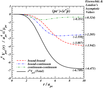
Figure 3: The quantity $r^{6}V_{\rm pol}(r)$ for different polarization potential components plotted as a function of $r$ in atomic units, for the $(pe^{-})$-$(e^{+}{\bar{p}})$ system. The numbers on the right are the $C_{6}$ coefficients from Eisenshitz and London for H₂ Eis28 .

Using the methods discussed in the last section, excitation matrix elements can be evaluated and the polarization potential $V_{\rm pol}$ from different contributions can be obtained. We show in Fig. 3 the quantity $r^{6}V_{\rm pol}(r)$ for the $(pe^{-})$-$(e^{+}{\bar{p}})$ system as a function of $r$, where $r^{6}V_{\rm pol}(r)$ from the bound-bound, bound-continuum, and continuum-continuum contributions are shown as the dashed, dash-dot and dash-dot-dot curves respectively. In these calculations, we include bound states up to $n=20$ in bound-bound calculations and $n=12$ in bound-continuum calculations. For calculations with continuum states, we include states up to $k=6$ atomic units.

We note in Fig. 3 that the curves of $r^{6}V_{\rm pol}$ flatten out at large values of $r$. This indicates that the attractive polarization potentials behave asymptotically as $-C_{6}/r^{6}$, the well-known van der Waals interaction at large distances between atoms. The asymptotic values of the $C_{6}$ from different contributions have been given along with the theoretical curves. They have also been obtained previously by Eisenschitz and London for H₂ Eis28 as listed on the right side of the figure. There is reasonable agreement between the $C_{6}$ values obtained in the present calculation and those of Eis28 . There is a small difference between the $C_{6}$ numbers involving continuum states with those of Eis28 . These small differences may arise from the fact that the curves involving continuum states have not yet become completely flattened and thus they may have not yet reached their asymptotic values.

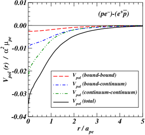
Figure 4: Components of the polarization potential and their total sum for the $(pe^{-})$-$(e^{+}{\bar{p}})$ system.

From these results, we note that at large separations, the bound-continuum contribution is much larger than the continuum-continuum contribution and is slightly smaller than the bound-bound contribution.

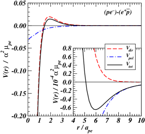
Figure 5: The direct, polarization and total interaction potentials for the $(pe^{-})$-$(e^{+}{\bar{p}})$ system.

The situation is different at small separations. We plot $V_{\rm pol}({r})$ as a function of $r$ in Fig. 4 for $(pe^{-})$-$(e^{+}\bar{p})$ and $r<5a_{pe}$. We find that the bound-bound contributions are smaller than the bound-continuum contributions, which in turn are smaller than the continuum-continuum contributions. The total polarization potential remains well-behaved at small $r$. Its magnitude is much smaller than the magnitude of the direct potential dominated by the attractive screened potential between $p$ and $\bar{p}$.

Having obtained both the direct and the total polarization potential, we can add them together to obtain the interaction potential $V(r)=V_{\rm dir}(r)+V_{\rm pol}(r)$. We show in Fig. 5 the interaction potential $V(r)$ and its components $V_{\rm dir}(r)$ and $V_{\rm pol}(r)$ for the $(pe^{-})$-$(e^{+}\bar{p})$ system. We note that for this case of large ratio of constituent masses $m_{1}/m_{2}$, the polarization potential is small compared to the direct potential at short distances and the total interaction is attractive at $r<a$. The repulsive barrier at $r\sim 2a$ that comes from the direct potential remains. The repulsive interaction decreases at larger separations. There is a pocket structure at $r\sim 6a_{pe}$ that is very shallow and arises from the interplay between the repulsion of like charges at intermediate distances and the attractive polarization potential Lee08 .

VIII The interaction potential in different systems

It is of interest to see how the interaction potential and its various components vary as a function of the constituent masses. The various potential components and the total polarization potential for $(\mu^{+}e^{-})$-$(e^{+}\mu^{-})$ in atomic units are very similar to those of $(pe^{-})$-$(e^{+}\bar{p})$ and will not be presented. The situation changes slightly for $(p\mu^{-})$-$(\mu^{+}\bar{p})$. We show the polarization potential components in Fig. 6 and the total interaction potential in Fig. 7 for $(p\mu^{-})$-$(\mu^{+}\bar{p})$. One notes from Fig.  6 that for this case with $m_{p}/m_{\mu}=8.88$, the bound-bound contributions to the polarization potential dominate over the bound-continuum or the continuum-continuum contributions. The results in Fig. 7 indicate that the total polarization potential is however small compared to the direct potential at $r<a$. The other features of the interaction potential is similar to those of the $(pe^{-})$-$(e^{+}{\bar{p}})$ system.

Figure 6: Components of the polarization potential and their total sum for the $(p\mu^{-})$-$(\mu^{+}{\bar{p}})$ system.

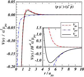
Figure 7: The direct potential, polarization potential, and the total interaction potential for the $(p\mu^{-})$-$(\mu^{+}{\bar{p}})$ system.

When the ratio of constituent masses $m_{1}/m_{2}$ approaches unity, the qualitative features of the different components change significantly. In Fig. 8, we show various components of the interaction potential for the $(\tau^{+}{\bar{p}})$-$(p\tau^{-})$ system, for which $m_{\tau}/m_{p}=1.89$. As one observes, the polarization potential is dominated by the bound-bound component while the bound-continuum and continuum-continuum contributions are small. The direct potential is much reduced compared to the case with large constituent mass ratios $m_{1}/m_{2}$ and is now of the same order of magnitude as the polarization potential.

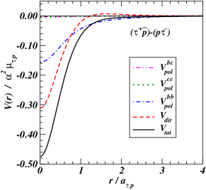
Figure 8: The direct potential, polarization potential, and the total potential for the $(\tau^{+}{\bar{p}})$-$(p\tau^{-})$ system.

IX Quantization of the four-body system

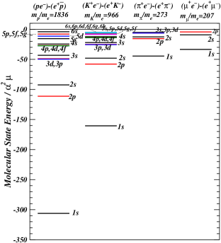
Figure 9: The eigenenergies of the molecular states states in $(pe^{-})$-$(e^{+}{\bar{p}})$, $(K^{+}e^{-})$-$(e^{+}K^{-})$, $(\pi^{+}e^{-})$-$(e^{+}\pi^{-})$, and $(\mu^{+}e^{-})$-$(e^{+}\mu^{-})$, in atomic units.

To study molecular states based on $A$ and $\bar{A}$ atoms as building blocks, we quantize the Hamiltonian for the four-body system by solving the Schrödinger equation (12). The states of the system depend not only on the interaction potential $V(r)$ but also on the reduced mass.

Because we use the atomic units of the $A(m_{1}m_{2})$ atom to measure our quantities, it is necessary to measure the reduced mass $\mu_{A{\bar{A}}}$ for molecular motion in units of $\mu_{12}$, as given by Eq. (18),

$$(\mu_{A{\bar{A}}}{\rm~{}in~{}atomic~{}units})=\frac{(m_{1}+m_{2})^{2}}{2m_{1}m_{2}}=\frac{(1+m_{1}/m_{2})^{2}}{2m_{1}/m_{2}}.$$ (49)

To provide a definite description of the constituents, we order the masses of the constituents such that $m_{1}$$>$$m_{2}$ and characterize the system by the ratio $m_{1}/m_{2}$.

In our problem, the use of the atomic units of $A$ and $\bar{A}$ as described in Section III brings us significant simplicity. We have just seen that the reduced mass in atomic units is a simple function of the constituent mass ratio $m_{1}/m_{2}$. It should also be realized that the interaction potential and its different components in atomic units depend only on the various coefficients $F_{A\bar{A}}$ or $f_{1,2,3,4}$, which are themselves ratios and are uniquely characterized by $m_{1}/m_{2}$. Therefore, the Coulomb four-body system in atomic units is completely characterized by $m_{1}/m_{2}$. Consequently, two different four-body systems with the same $m_{1}/m_{2}$ will have the same molecular state eigenenergies and eigenfunctions in atomic units. We can infer the stability of a molecule by studying the change of the molecular eigenenergies as a function of $m_{1}/m_{2}$.

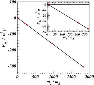
Figure 10: The eigenenergy of the $1s$ molecular state as a function of $m_{1}/m_{2}$.

We give in Table II the values of $m_{1}/m_{2}$, the reduced mass in atomic units of the $A$ atom, and the molecular state binding property, for many four-particle systems. The reduced mass decreases as $m_{1}/m_{2}$ decreases.

Table 2: Relationship between $m_{1}/m_{2}$, reduced mass, and the presence of bound molecular states in many four-body systems.

System		Reduced mass	Eigenenergy of
$A(m_{1}^{+}m_{2}^{-})$-${\bar{A}}({\bar{m}}_{2}^{+}{\bar{m}}_{1}^{-})$	$m_{1}/m_{2}$	in atomic units	1s molecular state
$(m_{1}>m_{2})$
$(pe^{-})$-$(e^{+}{\bar{p}})$	1836.2	919.1	-306.2
$(K^{+}e^{-})$-$(e^{+}K^{-})$	966.1	484.1	-160.6
$(\pi^{+}e^{-})$-$(e^{+}\pi^{-})$	273.1	137.6	-44.63
$(\mu^{+}e^{-})$-$(e^{+}\mu^{-})$	206.8	104.4	-33.52
$(p\mu^{-})$-$(\mu^{+}{\bar{p}})$	8.88	5.50	-0.540
$(K^{+}\mu^{-})$-$(\mu^{+}K^{-})$	4.67	3.44	-0.0239
$(\tau^{+}{\bar{p}})$-$(p\tau^{-})$	1.89	2.21	None

How does the interaction potential varies as $m_{1}/m_{2}$ decreases? For the case of $m_{1}/m_{2}\gg 1$, the interaction potential at small $r$ is dominated by the direct potential over the polarization potential. The total interaction potential is strongly attractive at small $r$. As $m_{1}/m_{2}$ decreases and approaches $1$, the direct potential is significantly reduced, and the interaction potential becomes dominated by the polarization potential. The net result is a decrease in the strength of the attractive interaction.

We solve the Schrödinger equation (12) to obtain the eigenstate energies $\epsilon$ for different molecular systems using the corresponding reduced masses and interaction potentials. The fourth column in Table II indicates whether bound states are present in various systems. There are bound states in $(pe^{-})$-$(e^{+}{\bar{p}})$, $(K^{+}e^{-})$-$(e^{+}K^{-})$, $(\pi^{+}e^{-})$-$(e^{+}\pi^{-})$, $(\mu^{+}e^{-})$-$(e^{+}\mu^{-})$, $(p\mu^{-})$-$(\mu^{+}{\bar{p}})$, and $(K^{+}\mu^{-})$-$(\mu^{+}K^{-})$. The results in Table II indicate that bound molecular states exist for four-particle systems if $m_{1}/m_{2}$ is greater than about 4 (or if the reduced mass is greater than or about 3 atomic units). The eigenenergies for many four-particle systems are shown in Fig. 9. We label eigenstates by the angular momentum and the principal quantum number, which is equal to the number of nodes plus $l+1$. The eigenenergies (measured in their corresponding atomic unit $\alpha^{2}\mu_{12}$) move up into the continuum as $m_{1}/m_{2}$ approaches unity and the reduced mass decreases.

We can examine the molecular state energies of $(pe^{-})$-$(e^{+}{\bar{p}})$ and compare them with those of a $p\bar{p}$ atom. For the $(pe^{-})$-$(e^{+}{\bar{p}})$ molecule, the molecular 1$s$ state energy is located at -306.2$\alpha^{2}\mu_{pe}$ and the $ns$ state is higher than the $np$ state, whereas the atomic $1s$ state energy for a $p\bar{p}$ atom is -459.5$\alpha^{2}\mu_{pe}$ and the $ns$ state has the same eigenenergy as the $np$ state. The differences in state energies and ordering arise because in the $(pe^{-})$-$(e^{+}{\bar{p}})$ system, the interaction potential at small $r$ is given by Eq. (33) (or Eq. (35)) that contains the first term of an attractive screened potential with a screening length $f_{1}a/2\sim a/2$. This screening length is so large compared to the $p\bar{p}$ Bohr radius that the attractive screened potential is nearly $-\alpha/r$ in character, as in a $p\bar{p}$ atom. However, there is an additional repulsive screened Coulomb interaction in Eq. (33) with a screening length $f_{2}a/2$ that is comparable to the $p\bar{p}$ Bohr radius. This repulsive screened Coulomb interaction arises because in the $(pe^{-})$-$(e^{+}{\bar{p}})$ molecule, the orbiting of the leptons with respect to the baryons leads to the motion of the baryons. As a consequence, the proton and the antiproton have a spatial distribution and the interaction between the charge distributions of the proton and the antiproton is reduced from their point-charged values. This additional repulsive screened Coulomb interaction in Eq. (33) raises the eigenenergy of $(pe^{-})$-$(e^{+}{\bar{p}})$ in the 1$s$ state molecular state relative to the eigenenergy of the $p\bar{p}$ atom in the $1s$ state, and the $ns$ state to lie higher than the $np$ state.

For $(p\mu^{-})$-$(\mu^{+}{\bar{p}})$ for which $m_{1}/m_{2}=8.88$, $1s$ state energy is at -0.5425 atomic units. The molecular state is weakly bound. For $(K^{+}\mu^{-})$-$(\mu^{+}K^{-})$ for which $m_{1}/m_{2}=4.67$, the $1s$ state energy lies at -0.0239 atomic units , which is just barely bound, indicating that $m_{1}/m_{2}\sim 4$ is the boundary between the region of bound and unbound molecular states. For $(\tau^{+}\bar{p})$-$(p\tau^{-})$ for which $m_{1}/m_{2}=1.89$, there is no bound molecular state.

We plot in Fig. 10 the eigenenergy of the molecular $1s$ state as a function of $m_{1}/m_{2}$. As one observes in Fig. 10 and Table II, the engenenergy varies approximately linearly as a function of $m_{1}/m_{2}$, with an intercept of $E=0$ at $m_{1}/m_{2}\sim 4$, indicating that bound molecular states are present for $m_{1}/m_{2}$ greater than about 4.

X Annihilation Lifetimes of Molecular States

Having located the energies of matter-antimatter molecules in various systems, we would like to calculate their annihilation lifetimes. The annihilation probability depends on many factors: the spatial factor of contact probability that is determined by the particle wave functions, the type of annihilating particles whether they are leptons or hadrons, and the spins of the annihilating pair if they are leptons. We shall discuss these different factors in turn.

X.1 Spatial Factor in Particle-Antiparticle Annihilation

In our matter-antimatter molecules, $m_{1}$-$m_{4}$ and $m_{2}$-$m_{3}$ are charge conjugate pairs which can annihilate. The total annihilation probability naturally comprises of $P_{14}$ for the annihilation of $m_{1}$ and $m_{4}$, and $P_{23}$ for the annihilation of $m_{2}$ and $m_{3}$. These spatial factors $P_{jk}$ can be obtained by approximating the constituent wave function to contain only the first term of the perturbative expansion in Eq. (10), as amplitudes of the excited states relative to the unperturbed states are small and the excited states have greater spatial extensions that suppress the annihilation probabilities.

We shall limit our attention to the annihilation of $s$-wave molecular states, which dominates the annihilation process. By the term “annihilation” in the present work, we shall refer to the annihilation in the $s$-wave molecular states only. The probabilities for the annihilation in higher angular momentum states are higher order in $\alpha$ Cra06 and involve not only derivatives of the molecular wave function at the origin but also complicated angular momentum couplings. They will need to be postponed to a later date.

We shall calculate the spatial factor $P_{jk}$ for the molecular ($s$-wave) state $\psi({\hbox{\boldmath${r}$}})$ built on $A_{\nu}(m_{1}m_{2})$ and ${\bar{A}}_{\nu^{\prime}}(m_{3}m_{4})$ atoms. It is quantitatively defined as the probability per unit volume for finding the conjugate $m_{j}$-$m_{k}$ pair to be at the same spatial location, in the molecular ($s$-wave) state $\psi({\hbox{\boldmath${r}$}})$ with $A_{\nu}(m_{1}m_{2})$ and ${\bar{A}}_{\nu^{\prime}}(m_{3}m_{4})$ atoms. It is the expectation value of $\delta({\hbox{\boldmath${r}$}}_{jk})$,

$$P_{jk} = \int d{\hbox{\boldmath${r}$}}d{\hbox{\boldmath${r}$}}_{12}d{\hbox{\boldmath${r}$}}_{34}A_{\nu}^{*}({\hbox{\boldmath${r}$}}_{12}){\bar{A}}_{\nu^{\prime}}^{*}({\hbox{\boldmath${r}$}}_{34})\psi^{*}({\hbox{\boldmath${r}$}})\delta({\hbox{\boldmath${r}$}}_{jk})\psi({\hbox{\boldmath${r}$}})A_{\nu}({\hbox{\boldmath${r}$}}_{12}){\bar{A}}_{\nu^{\prime}}({\hbox{\boldmath${r}$}}_{34}).~{}~{}~{}~{}~{}$$ (50)

We shall consider molecular states built on $\nu=\nu^{\prime}=0$, then

$$P_{jk} = \int d{\hbox{\boldmath${r}$}}|\psi({\hbox{\boldmath${r}$}})|^{2}\langle A_{0}{\bar{A}}_{0}|\delta({\hbox{\boldmath${r}$}}_{jk})|A_{0}{\bar{A}}_{0}\rangle$$ (51)

$$= \int d{\hbox{\boldmath${r}$}}|\psi({\hbox{\boldmath${r}$}})|^{2}\langle A_{0}{\bar{A}}_{0}|\delta({\hbox{\boldmath${r}$}}+F_{A}(jk){\hbox{\boldmath${r}$}}_{12}+F_{B}(jk){\hbox{\boldmath${r}$}}_{34})|A_{0}{\bar{A}}_{0}\rangle,~{}~{}~{}$$

in which $\langle A_{0}{\bar{A}}_{0}|\delta({\hbox{\boldmath${r}$}}_{jk})|A_{0}{\bar{A}}_{0}\rangle$ has the same structure as $V_{\rm dir}$ except that $v_{jk}({\hbox{\boldmath${r}$}}_{jk})$ is replaced by a delta function. For this case with $\nu=\nu^{\prime}=0$, the sign of $F_{A,{\bar{A}}}$ does not matter, and we can just use $f_{A,{\bar{A}}}$ for $F_{A,\bar{A}}$. Similar to Eq. (32), we have

$$\langle A_{0}{\bar{A}}_{0}|\delta(\hbox{\boldmath${r}$}_{jk})|A_{0}{\bar{A}}_{0}\rangle=\int\frac{d\hbox{\boldmath${p}$}}{(2\pi)^{3}}e^{i\hbox{\boldmath${p}$}\cdot\hbox{\boldmath${r}$}}\frac{16}{((pf_{A}a_{0})^{2}+4)^{2}}\frac{16}{((pf_{\bar{A}}a_{0})^{2}+4)^{2}}.~{}~{}~{}~{}~{}$$ (52)

For both $\{jk\}=\{14\}$ and $\{23\}$, $f_{\bar{A}}(jk)=f_{A}(jk)$, and we get

$$D_{jk}({\hbox{\boldmath${r}$}}) \equiv \langle A_{0}{\bar{A}}_{0}|\delta_{jk}(\hbox{\boldmath${r}$}_{jk})|A_{0}{\bar{A}}_{0}\rangle$$ (53)

$$= \frac{e^{-\lambda_{A}(jk)r}}{4\pi}\frac{[\lambda_{A}(jk)]^{3}}{48}\left\{[\lambda_{A}(jk)r]^{2}+3\lambda_{A}(jk)r+3\right\},$$

where

$$\lambda_{A}(jk) = \frac{2}{f_{A}(jk)a},$$

$$f_{A}(14) = \frac{m_{2}}{m_{1}+m_{2}},~{}~{}~{}~{}~{}~{}f_{A}(23)=\frac{m_{1}}{m_{1}+m_{2}}.$$

Eq. (51) becomes

$$P_{jk}=\int d{\hbox{\boldmath${r}$}}|\psi({\hbox{\boldmath${r}$}})|^{2}D_{jk}({\hbox{\boldmath${r}$}}).$$ (54)

As the wave function $\psi({\hbox{\boldmath${r}$}})$ has been obtained from our solution of the Schrödinger equation, the spatial factors can be calculated numerically.

Following Wheeler Whe46 , we can consider an antiparticle $\bar{m}$ to be at rest while its conjugate particle $m$ sweeps by with a annihilation cross section $\sigma_{\rm ann}^{m\bar{m}}$ at a velocity $v$, clearing a volume $\sigma_{\rm ann}^{m\bar{m}}v$ per unit time. The probability of finding the pair of particles $j$ and $k$ to be in contact, per unit spatial volume, is $P_{jk}$. As a consequence, the number of particle-antiparticle contacts per unit time, which is equal to the rate of annihilation $w_{jk}^{m\bar{m}}$, is given by

$$w_{jk}^{m\bar{m}} = \sigma_{\rm ann}^{m\bar{m}}v\times P_{jk}.$$ (55)

X.2 Annihilation of Lepton Constituents

The matter-antimatter molecules we have been considering consist of both leptons and hadrons. The annihilation cross section $\sigma_{\rm ann}^{m\bar{m}}$ depends on the particle type and the total spin of the annihilating pair. We shall discuss the annihilation of lepton pairs in this subsection. The annihilation of hadron pairs will be discussed in the next subsection.

The mechanism for the annihilation of a lepton pair is well known Whe46 ; Ber82 . It proceeds through the electromagnetic interaction with the fine-structure coupling constant $\alpha$ and the emission of two or three photons. A lepton pair with spin $S$=$0$ can annihilate only into two photons, and a lepton pair with spin $S$=$1$ can annihilate only into three photons Whe46 . The lepton pair annihilation cross section multiplied by velocity $v$ is given by Whe46 ; Ber82

$$\sigma_{S_{jk}=0}^{l\bar{l}}v~{}~{}({\rm for~{}annihilation~{}into~{}2~{}photons})=\pi\left(\frac{\alpha}{\mu c^{2}}\right)^{2}$$ (56)

$$\sigma_{S_{jk}=1}^{l\bar{l}}v~{}~{}({\rm for~{}annihilation~{}into~{}3~{}photons})=\frac{4(\pi^{2}-9)}{9}\alpha\left(\frac{\alpha}{\mu c^{2}}\right)^{2}$$ (57)

As a consequence, the rates of annihilation of a lepton pair in the singlet and triplet states are Whe46 ; Ber82

$$w_{S_{jk}=0}^{l\bar{l}}({\rm annihilation~{}into~{}2~{}photons}) = \pi\left(\frac{\alpha}{\mu c^{2}}\right)^{2}P_{jk}$$ (58)

$$w_{S_{jk}=1}^{l\bar{l}}({\rm annihilation~{}into~{}3~{}photons}) = \frac{4(\pi^{2}-9)}{9}\alpha\left(\frac{\alpha}{\mu c^{2}}\right)^{2}P_{jk}~{}~{}~{}~{}~{}~{}~{}~{}~{}~{}$$ (59)

Thus, to obtain the rate of annihilation of a lepton-antilepton pair $\{jk\}$ in a molecular state, it is necessary to find out the probabilities for the pair to be in different $S_{jk}$ pair spin states in the molecule.

Our molecular states have been constructed by building them with $A(12)$ and ${\bar{A}}(34)$ atoms in their ground states. As we restrict our considerations to only $s$-wave molecular states, there is no orbital angular momentum between the $A$ and $\bar{A}$ atoms. In picking the lepton $l$ from atom $A$ and the antilepton $\bar{l}$ from the other atom $\bar{A}$, the probabilities for different lepton-antilepton pair spin states depend on the angular momentum coupling of the lepton-antilepton pair with the remaining constituents.

We consider first the case when the remaining constituents are also fermions. The four constituents can be labeled as $\{m_{1}$=$f,m_{2}$=$l,m_{3}$=${\bar{l}},m_{4}$=${\bar{f}}\}$. Each of the $A(12)$ and ${\bar{A}}(34)$ atoms has an atomic spin $S_{12}^{A},S_{34}^{\bar{A}}=0$ or 1. As a consequence, the $s$-wave molecular state has a total molecular spin $S_{\rm tot}^{A\bar{A}}=0,1,$ or 2. By the definition of the 9-$j$ symbols Des63 , the probability amplitude for the occurrence of fermion-antifermion spin states of $S_{14}^{f\bar{f}}$ and $S_{32}^{l\bar{l}}$ in a state with atom spins $S_{12}^{A}$ and $S_{34}^{\bar{A}}$ and molecular spin $S_{\rm tot}^{A\bar{A}}$ is

$$\langle S_{14}^{f\bar{f}}S_{23}^{l\bar{l}};S_{\rm tot}^{A\bar{A}}|S_{12}^{A}S_{43}^{\bar{A}};S_{\rm tot}^{A\bar{A}}\rangle$$

$$=\sqrt{(2S_{14}^{f\bar{f}}+1)(2S_{23}^{l\bar{l}}+1)(2S_{12}^{A}+1)(2S_{43}^{\bar{A}}+1)}\left\{\begin{matrix}s_{1}&s_{2}&S_{12}^{A}\cr s_{4}&s_{3}&S_{43}^{\bar{A}}\cr S_{14}^{f\bar{f}}&S_{23}^{l\bar{l}}&S_{\rm tot}^{A\bar{A}}\end{matrix}\right\},~{}~{}~{}~{}$$ (60)

where $s_{1}$=$s_{2}$=$s_{3}$=$s_{4}$=1/2. The probability $|\langle S_{14}^{f\bar{f}}S_{23}^{l\bar{l}};S_{\rm tot}^{A\bar{A}}|S_{12}^{A}S_{43}^{\bar{A}};S_{\rm tot}^{A\bar{A}}\rangle|^{2}$ for different atomic spins of $S_{12}^{A}$ and $S_{43}^{\bar{A}}$ combining into different $S_{14}^{f\bar{f}}$ and $S_{23}^{l\bar{l}}$, for a fixed total molecular spin $S_{\rm tot}$, are given in Table III.

Table 3: Probabilities for different atomic spins of $S_{12}^{A}$ and $S_{34}^{\bar{A}}$, combining into $S_{14}^{f\bar{f}}$ and $S_{23}^{l\bar{l}}$, for a fixed total molecular spin $S_{\rm tot}^{A\bar{A}}$.

	$S_{12}^{A}$	$S_{34}^{\bar{A}}$	$S_{14}^{f\bar{f}}$	$S_{23}^{l\bar{l}}$	probability
$S_{\rm tot}^{{}_{A\bar{A}}}=2$	1	1	1	1	1
$S_{\rm tot}^{{}_{A\bar{A}}}=1$	1	1	1	0	1/2
	1	1	0	1	1/2
$S_{\rm tot}^{{}_{A\bar{A}}}=1$	1	0	1	1	1/2
	1	0	1	0	1/4
	1	0	0	1	1/4
$S_{\rm tot}^{{}_{A\bar{A}}}=1$	0	1	1	1	1/2
	0	1	1	0	1/4
	0	1	0	1	1/4
$S_{\rm tot}^{{}_{A\bar{A}}}=0$	1	1	1	1	1/4
	1	1	0	0	3/4
$S_{\rm tot}^{{}_{A\bar{A}}}=0$	0	0	1	1	3/4
	0	0	0	0	1/4

Table 4: The $s$-wave $(\mu^{+}e^{-})$-$(e^{+}\mu^{-})$ molecular state energies and annihilation lifetimes in different $S_{\rm tot}^{A\bar{A}}$, $S_{12}^{A}$, and $S_{34}^{\bar{A}}$ spin configurations.

$(\mu^{+}e^{-})$-$(e^{+}\mu^{-})$	Energy($\alpha^{2}\mu$)				Annihilation
Molecular state		$S_{\rm tot}^{{}_{{}_{A\bar{A}}}}$	$S_{12}^{A}$	$S_{34}^{{}_{\bar{A}}}$	Lifetime $\tau_{\rm ann}$(sec)
1$s$	-33.5	2	1	1	0.861$\times 10^{-8}$
		1	1	1	0.154$\times 10^{-10}$
		1	1	0	0.308$\times 10^{-10}$
		1	0	1	0.308$\times 10^{-10}$
		0	1	1	0.103$\times 10^{-10}$
		0	0	0	0.308$\times 10^{-10}$
2$s$	-9.30	2	1	1	0.405$\times 10^{-7}$
		1	1	1	0.726$\times 10^{-10}$
		1	1	0	0.145$\times 10^{-9}$
		1	0	1	0.145$\times 10^{-9}$
		0	1	1	0.484$\times 10^{-10}$
		0	0	0	0.145$\times 10^{-9}$

By taking into account spin probabilities, the total rate of annihilation for matter-antimatter molecules consisting of 4 fermions with total molecular spin $S_{\rm tot}^{A\bar{A}}$, initial atomic spins $S_{12}^{A}$ and $S_{34}^{\bar{A}}$ is

$$w_{\rm ann}(S_{12}^{A}S_{34}^{\bar{A}}S_{\rm tot}^{A\bar{A}})=\sum_{S_{14}S_{23}}|\langle S_{14}S_{23};S_{\rm tot}^{A\bar{A}})|S_{12}^{A}S_{43}^{\bar{A}};S_{\rm tot}^{A\bar{A}}\rangle|^{2}[w_{{}_{S_{14}}}^{f\bar{f}}+w_{{}_{S_{23}}}^{l\bar{l}}],$$ (61)

where for lepton annihilations $w_{{}_{S_{23}}}^{l\bar{l}}$ is given by Eqs. (58) and (59). The annihilation lifetime is then given by

$$\tau_{\rm ann}(S_{12}^{A}S_{34}^{\bar{A}}S_{\rm tot}^{A\bar{A}})=\frac{1}{w_{\rm ann}(S_{12}^{A}S_{34}^{\bar{A}}S_{\rm tot}^{A\bar{A}})}$$ (62)

The rate of annihilation of the $(\mu^{+}e^{-})$-$(\mu^{+}e^{+})$ molecule in its $ns$ states can be calculated from Eq. (61) by identifying $f$=$\mu$ and $l$=$e$. The results for the annihilation lifetimes are shown in Table IV where we list the $(\mu^{+}e^{-})$-$(e^{+}\mu^{-})$ molecular state energies, the molecular spins $S_{\rm tot}^{A\bar{A}}$, the atomic spins $S_{12}^{A}$, $S_{34}^{\bar{A}}$ and the annihilation lifetimes $\tau_{\rm ann}$. In calculating the annihilation lifetimes in their physical units, we have used Table I to convert atomic units to physical units.

The $(\mu^{+}e^{-})$-$(e^{+}\mu^{-})$ molecular states with spin $S_{\rm tot}^{A\bar{A}}$=2 have the longest annihilation lifetimes, corresponding to lepton-antilepton pairs in their spin triplet states. The molecular 1$s$ and $2s$ $S_{\rm tot}^{A\bar{A}}=2$ states have annihilation lifetimes of $0.861\times 10^{-8}$ and $0.405\times 10^{-7}$ sec, respectively. Their relatively long annihilation lifetimes may make them accessible for experimental observations.

X.3 Annihilation of Hadron Constituents

Hadrons are composite particles consisting of quarks and/or antiquarks whose quantized masses are governed by non-perturbative quantum chromodynamics. As a consequence, there are no simple selection rules for hadron annihilation similar to those for the annihilation of leptons.

The lightest quantized hadrons are pions. Because of the difference in their masses, the annihilation of heavier hadron pairs such as $p\bar{p}$ and $K^{+}K^{-}$ differ from the annihilation of $\pi^{+}\pi^{-}$. The annihilations of $p\bar{p}$ and $K^{+}K^{-}$ pairs proceed through strong interactions as many pairs of pions and other hadrons can be produced. In contrast, a $\pi^{+}\pi^{-}$ pair can annihilate through strong interactions only when its center-of-mass energy $\sqrt{s}$ exceeds the threshold of $4m_{\pi}$, with the production of an additional pion pair. For pions in a matter-antimatter molecule, the momentum of the pion is of order $\alpha m_{\pi}$ and it has energy much below the strong-interaction annihilation threshold. We can infer that pions in a matter-antimatter molecule annihilate predominantly through the electromagnetic interaction with the emission of photons or dileptons.

Figure 11: $p\bar{p}$ total cross section in mb as a function of $p_{\rm lab}$

We shall first discuss the annihilation of heavy hadrons such as $p\bar{p}$ and $K^{+}K^{-}$. We envisage that these hadrons annihilate essentially through a geometrical consideration depicting the occurrence of annihilations within a geometrical area $\sigma_{0}$, with important initial state interactions that lead to a Gamow-factor $1/v$ type enhancement at low energies Cha95 ; Won97 . We can therefore parametrized the annihilation cross section as

$$\sigma_{\rm ann}=\frac{\sigma_{0}}{v},$$ (63)

where $v$ is the relative velocity between the colliding hadrons. From the PDG data PDG10 , the total and elastic $p\bar{p}$ cross sections in Fig. 11 obey the following relationship:

$$\sigma_{\rm total}^{p\bar{p}}=\sigma_{\rm elast}^{p\bar{p}}+\frac{50{\rm mb}}{v},$$ (64)

where

$$v=\frac{p_{\rm lab}}{\sqrt{p_{\rm lab}^{2}+m_{p}^{2}}}.$$ (65)

• As $p\bar{p}$ inelastic cross section is the same as the $p\bar{p}$ annihilation cross section, the experimental data gives $\sigma_{0}=50$ mb, and

$$\sigma_{\rm ann}^{p\bar{p}}v=\sigma_{0}=50{\rm~{}mb}.$$ (66)

For other systems, we can use the additive quark model Won94 ; Won94a to infer that

$$\sigma_{\rm ann}^{h\bar{h}}\propto n_{q}^{h}\times n_{q}^{\bar{h}},$$ (67)

where $n_{q}^{h}$ and $n_{q}^{\bar{h}}$ are the number of quarks in $h$ and $\bar{h}$. We get

$$\sigma_{\rm ann}^{h\bar{h}}v\sim\frac{n_{q}^{h}n_{q}^{\bar{h}}}{9}{50{\rm mb}}.$$ (68)

Consequently, the rate of annihilation of constituents 1 and 4 through strong interactions per unit time is

$$w_{14}^{h\bar{h}} = \frac{n_{q}^{h}n_{q}^{\bar{h}}}{9}50{\rm mb}\times P_{14},~{}~{}~{}\{h\bar{h}\}=\{p\bar{p}\}{\rm~{}or~{}}\{K^{+}K^{-}\}.$$ (69)

• In the $(pe^{-})$-$(e^{+}{\bar{p}})$ molecule, there are two leptons and two baryons. The spins of the four fermions are coupled together and we have

$$w_{\rm ann}(S_{12}^{A}S_{34}^{\bar{A}}S_{\rm tot}^{A\bar{A}})=w_{14}^{p\bar{p}}+\sum_{S_{14}^{p\bar{p}}S_{23}^{e^{+}e^{-}}}|\langle S_{14}^{p\bar{p}}S_{23}^{e^{+}e^{-}};S_{\rm tot}^{A\bar{A}}|S_{12}^{A}S_{43}^{\bar{A}};S_{\rm tot}^{A\bar{A}}\rangle|^{2}w_{{}_{S_{23}}}^{e^{-}e^{+}}.$$ (70)

In the $(K^{+}e^{-})$-$(e^{+}K^{-})$ molecule, there is a lepton pair and a $K$-$\bar{K}$ pair. As the kaons have spin zero, the molecular spin $S_{\rm tot}$ comes only from the leptons and we have

$$w_{\rm ann}(S_{\rm tot})=w_{14}^{K^{+}K^{-}}+w_{S_{\rm tot}}^{e^{+}e^{-}}.$$ (71)

In practice, for the molecular $ns$ states we have considered, the rate of hadron annihilation is much greater than the rate of lepton annihilation, if the hadrons can annihilate through strong interactions. In this case, because of the dominance of the hadron annihilation through strong interactions, the total annihilation rate is essentially independent of the spin of the molecule $S_{\rm tot}$.

For the case involving $\pi^{+}$ and $\pi^{-}$ constituents, annihilation cannot proceed through strong interactions as the pion energies are below the inelastic threshold. The pion pair can annihilate into photons and dileptons. Because the $\pi^{+}$-$\pi^{-}$ system has the same total angular momentum and parity quantum numbers as the spin singlet state of a lepton pair, and the Feynman diagrams for the emission of two photons in QED for $l+\bar{l}\to 2\gamma$ and $\pi^{+}+\pi^{-}\to 2\gamma$ have the same structure, we can approximate the $\pi^{+}$+$\pi^{-}$$\to 2\gamma$ cross section to be the same form as the spin-singlet $l+{\bar{l}}\to 2\gamma$ cross section in Eq. (56),

$$\sigma_{\rm ann}^{\pi^{+}\pi^{-}}v_{\pi^{+}\pi^{-}}\sim\pi\left(\frac{\alpha}{\mu_{\pi\pi}c^{2}}\right)^{2}.$$ (72)

The cross section for pion annihilation into dileptons [as given by Eq. (14.33) of Ref. Won94 ] is of order $\alpha^{3}$ for pions with momentum $p\sim\alpha m_{\pi}$. We can neglect the dilepton contribution from $\pi^{+}$+$\pi^{-}$$\to l$+$\bar{l}$ in the present estimate. Consequently, the rate of annihilating pion constituents 1 and 4 by electromagnetic interactions per unit time is

$$w_{14}^{\pi^{+}\pi^{-}} = \pi\left(\frac{\alpha}{\mu_{\pi\pi}c^{2}}\right)^{2}\times P_{14}.$$ (73)

• In the $(\pi^{+}e^{-})$-$(e^{+}\pi^{-})$ molecule, there is a lepton pair and a $\pi^{+}$-$\pi^{-}$ pair. As the pions have spin zero, the molecular spin comes only from the leptons. For the $(\pi^{+}e^{-})$-$(e^{+}\pi^{-})$ molecule, we have

$$w_{\rm ann}(S_{\rm tot})=w_{14}^{\pi^{+}\pi^{-}}+w_{S_{\rm tot}}^{e^{+}e^{-}}.$$ (74)

Because the annihilation of both the lepton pair and the pion pairs are electromagnetic in origin, they are comparable in magnitude. The annihilation rate depends on the spin of the molecule $S_{\rm tot}$.

Table 5: Molecular $1s$ state energies and annihilation lifetimes for $(pe^{-})$-$(e^{+}\bar{p})$, $(p\mu^{-})$-$(\mu^{+}\bar{p})$, $(K^{+}e^{-})$-$(e^{+}K^{-})$, $(K^{+}\mu^{-})$-$(\mu^{+}K^{-})$ and $(\pi^{+}e^{-})$-$(e^{+}\pi^{-})$.

System	State	Energy($\alpha^{2}\mu$)	Annihilation
			Lifetime(sec)
$(pe^{-})$-$(e^{+}\bar{p})$	1$s$	-306.208	0.549$\times 10^{-17}$
	2$s$	-92.565	0.347 $\times 10^{-17}$
	3$s$	-43.255	0.107$\times 10^{-15}$
	4$s$	-24.595	0.244$\times 10^{-15}$
	5$s$	-15.595	0.464$\times 10^{-15}$
	6$s$	-4.094	0.259$\times 10^{-14}$
$(p\mu^{-})$-$(\mu^{+}{\bar{p}})$	1$s$	-0.540	0.532$\times 10^{-17}$
$(K^{+}e^{-})$-$(e^{+}K^{-})$	1s	-160.601	0.853$\times 10^{-16}$
	2$s$	-48.108	0.526$\times 10^{-15}$
	3$s$	-22.141	0.166$\times 10^{-14}$
	4$s$	-12.316	0.372$\times 10^{-14}$
	5$s$	-7.581	0.715$\times 10^{-14}$
	6$s$	-4.947	0.122$\times 10^{-13}$
$(K^{+}\mu^{-})$-$(\mu^{+}K^{-})$	1$s$	-0.0239	0.154$\times 10^{-15}$
$(\pi^{+}e^{-})$-$(e^{+}\pi^{-})$	1$s$	-44.625	($S_{\rm tot}$=0) 0.592$\times 10^{-11}$
			($S_{\rm tot}$=1) 0.622$\times 10^{-11}$
	2$s$	-12.698	($S_{\rm tot}$=0) 0.298$\times 10^{-10}$
			($S_{\rm tot}$=1) 0.392$\times 10^{-10}$
	3$s$	-5.341	($S_{\rm tot}$=0) 0.616$\times 10^{-10}$
			($S_{\rm tot}$=1) 0.121$\times 10^{-9}~{}$

In Table V, we list the $l$=$0$ molecular states, their energies, and their lifetime for $(pe^{-})$-$(e^{+}\bar{p})$, $(p\mu^{-})$-$(\mu^{+}\bar{p})$, $(K^{+}e^{-})$-$(e^{+}K^{-})$, $(K^{+}\mu^{-})$-$(\mu^{+}K^{-})$, and $(\pi^{+}e^{-})$-$(e^{+}\pi^{-})$. We observe that the annihilation lifetimes are short for the $(pe^{+})$-$(e^{+}\bar{p})$ states, of the order of $10^{-15}$-$10^{-18}$ sec, increasing to order $10^{-10}$-$10^{-11}$ sec for $(\pi^{+}e^{-})$-$(e^{+}\pi^{-})$ states.

XI Summary and Discussions

To examine the stability of matter-antimatter molecules with constituents $(m_{1}^{+}m_{2}^{-}{\bar{m}}_{2}^{+}{\bar{m}}_{1}^{-})$ and $m_{1}$$>$$m_{2}$, we reduce the four-body problem into a simpler two-body problem. This is achieved by breaking up the four-body Hamiltonian into the unperturbed Hamiltonians of two atoms $A(m_{1}^{+}m_{2}^{-})$ and ${\bar{A}}({\bar{m}}_{2}^{+}{\bar{m}}_{1}^{-})$, plus residual interactions and the kinetic energies of the atoms. The unperturbed Hamiltonians of the two atoms can be solved exactly. Molecular states can be constructed by using the atoms $A$ and $\bar{A}$ as simple building blocks. The interaction potential $V({\hbox{\boldmath${r}$}})$ between the atoms is then the sum of the direct potential $V_{\rm dir}({\hbox{\boldmath${r}$}})$ arising from the interaction between the constituents and the polarization potential $V_{\rm pol}({\hbox{\boldmath${r}$}})$ arising from the virtual excitation of the atomic states in the presence of the other atom. The eigenenergies of the molecular states can be obtained by quantizing the four-particle Hamiltonian Won04 .

The Coulomb four-body system in atomic units of $A$ and $\bar{A}$ atoms is completely characterized by $m_{1}/m_{2}$. Consequently, two different four-body systems with the same $m_{1}/m_{2}$ will have the same molecular state eigenenergies and eigenfunctions in atomic units. We can infer the stability of a molecule by studying the change of the molecular eigenenergies as a function of $m_{1}/m_{2}$.

The effective reduced mass of $A(m_{1}^{+}m_{2}^{-})$-${\bar{A}}({\bar{m}}_{2}^{+}{\bar{m}}_{1})$ for molecular motion is large when $m_{1}/m_{2}\gg 1$ and decreases as $m_{1}/m_{2}$ approaches unity. The relative importance of the direct and polarization potential also changes with $m_{1}/m_{2}$. For a matter-antimatter molecule with $m_{1}/m_{2}\gg 1$, we find that the direct potential dominates in regions of $r<a$ and gives rise to deeply bound molecular states. As $m_{1}/m_{2}$ approaches unity, the magnitude of $V_{\rm dir}$ decreases and the polarization potential by itself is too weak to hold a bound state. As a consequence, the state energies (in atomic units) rises and comes up to the continuum as $m_{1}/m_{2}$ approaches the unity limit.

We find that matter-antimatter molecules possess bound states if $m_{1}/m_{2}$ is greater than about 4. This stability condition suggests that the binding of matter-antimatter molecules is a rather common phenomenon. This molecular stability condition is satisfied, and many bound molecular states of different quantum numbers are found, in many four-body systems: $(\mu^{+}e^{-})$-$(e^{+}\mu^{-})$, $(\pi^{+}e^{-})$-$(e^{+}\pi^{-})$, $(K^{+}e^{-})$-$(e^{+}K^{-})$, $(pe^{-})$-$(e^{+}\bar{p})$, $(p\mu^{-})$-$(\mu^{+}{\bar{p}})$, and $(K^{+}\mu^{-})$-$(\mu^{+}K^{-})$. Bound molecular states are not found in $(\tau^{+}{\bar{p}})$-$(p\tau^{-})$ which has $m_{1}/m_{2}=1.89$.

When one applies the stability condition to the $(e^{+}e^{-})$-$(e^{-}e^{+})$ system, one may naively infer at first that the $(e^{+}e^{-})$-$(e^{-}e^{+})$ system will not hold a bound state. On the other hand, bound $(e^{+}e^{-})^{2}$ molecular state has been experimentally observed Cas07 , and the binding energy has been calculated theoretically to be 0.016 a.u. relative to two $(e^{+}e^{-})$ atoms Koz93 . It should however be realized that the stability condition we have obtained applies to four-body systems with distinguishable constituents without identical particles. For systems with identical particles such as the $(e^{+}e^{-})^{2}$ system, it is necessary to take into account the antisymmetry of the many body wave function with respect to the exchange of the pair of identical particles. Depending on the spin symmetry of the identical particle pair in question, the symmetry or antisymmetry with respect to the spatial exchange of the pair will lead to a lowering or raising of the energy of the state. The identical particles in the bound $(e^{+}e^{-})^{2}$ system leading to the bound state have been selected to be spatially symmetric states Whe46 ; Koz93 , which corresponds to spin-antisymmetric with respect to the exchange of the pair of identical particles Koz93 . As a consequence, their spatial symmetry lowers the state energy relative to the state energy when there is no such a symmetry. The small value of the theoretical binding energy (0.016 a.u. Koz93 ) suggests the occurrence of such a lowering of the energy from the unbound to the bound energy region. In order to confirm this suggestion, it will be of interest in future work to extend the present formulation to include the case with identical particles and their exchange symmetries. How the additional symmetry considerations may modify the stability of those molecules with identical particles is worthy of future investigations. The states we have obtained may not contain all the correlations. Additional correlations may be included by adding correlation factors and using the solution of the present investigation as doorway states. Future addition of correlations superimposing on the states we have obtained will be of interest.

We can divide the annihilation lifetimes of matter-antimatter molecules into different groups that correlate with the types of constituents. Those molecules constructed from different leptons have the longest annihilation lifetimes, of the order of $10^{-8}$-$10^{-11}$ sec, depending on the spins of the molecular state. The second group involves leptons and pions in which the pions cannot annihilate through strong interactions and can annihilate only through the electromagnetic interactions. The annihilation lifetimes are of order $10^{-10}$-$10^{-11}$ sec. Molecular states containing kaons have annihilation lifetimes of order $10^{-14}$-$10^{-16}$ sec while those containing proton and antiproton $10^{-15}$-$10^{-18}$ sec. The relatively long annihilation lifetimes for leptonic $(\mu^{+}e^{-})$-$(e^{+}\mu^{-})$ molecules may make them accessible for experimental detection.

We have examined only molecular states constructed from the $A\bar{A}$ family in which the building-block atoms $A_{0}$ and ${\bar{A}}_{0}$ are in their ground states. We can likewise construct in future work states in the $A\bar{A}$ family in which $A$ and $\bar{A}$ are in their excited states. These states will have different interatomic interactions, obey different stability conditions, and have different properties with regard to annihilation and production. In another future direction of extension, we can also construct molecular states based on the $M\bar{M}$ family, using states of $M(m_{1}^{+}\bar{m}_{1}^{-})$ and ${\bar{M}}({\bar{m}}_{2}^{+}m_{2}^{-})$ as building blocks. The $A\bar{A}$ molecular states and the $M\bar{M}$ molecular states have different topological structures and properties. Molecular states built on different branches of the family tree will likely retain some of their family characteristics. These possibilities bring into focus the rich degrees of freedom and the vast varieties of states that need to be sorted out in the Coulomb four-body problem associated with matter-antimatter molecules.

In addition to the problem of molecular states as a structure problem investigated here, future theoretical and experimental studies should also be directed to the question of production and detection methods from reaction points of view. While the observation of new matter-antimatter molecules may be a difficult task, the prospect of classifying the $(m_{1}^{+}m_{2}^{-}{\bar{m}_{2}}^{-}{\bar{m}}_{2}^{+})$ system into the genealogy of families and basic building blocks, if it is at all possible, will bring us to a better understanding of the complexity of the spectrum that is associated with the complicated four-body problem opened up by the pioneering work of Wheeler Whe46 .

Appendix A Evaluation of the Matrix Element
$\langle A_{\lambda}{\bar{A}}_{\lambda^{\prime}}|v(\hbox{\boldmath${r}$}_{jk})|A_{0}{\bar{A}}_{0}\rangle$

The evaluation of the excitation transition matrix element requires first the Fourier transform of the transition density. The transition density for the excitation from the ground $|100\rangle$ state to the excited $|n1m\rangle$ state is

$$\rho_{n1m,100}({\bf r}) = \psi_{n1m}^{*}({\hbox{\boldmath${r}$}})\psi_{100}({\hbox{\boldmath${r}$}})$$ (75)

$$= \frac{N_{10}N_{n1}}{\sqrt{4\pi}}\exp\left\{-\frac{2r(n+1)}{2na_{0}}\right\}\left(\frac{2r}{na_{0}}\right)L_{n-2}^{3}(\frac{2r}{na_{0}})Y_{1m}^{*}(\theta,\phi).~{}~{}~{}~{}~{}~{}$$

Making the scale transformation $r=r^{\prime}/(n+1)=r^{\prime}\beta$, we have

$$\rho_{n1m,100}({\bf r})=\frac{N_{10}N_{n1}}{\sqrt{4\pi}}\exp\left\{-\frac{2r^{\prime}}{2na_{0}}\right\}\left(\frac{2r^{\prime}}{na_{0}}\right)\beta L_{n-2}^{3}\left(\frac{2r^{\prime}}{na_{0}}\beta\right)Y_{1m}^{*}(\theta,\phi).$$ (76)

We can expand $L_{j}^{\alpha}(\beta x)$ as a sum over Laguerre polynomials $L_{j-\kappa}^{\alpha}(x)$ as given in Eq. (22.12.6), page 785 in Abr70 ,

$$L_{j}^{\alpha}(\beta x)=\sum_{\kappa=0}^{j}\left(\begin{matrix}j+\alpha\cr\kappa\end{matrix}\right)\beta^{j-\kappa}(1-\beta)^{\kappa}L_{j-\kappa}^{\alpha}(x).$$ (77)

The transition density becomes

$$\rho_{n1m,100}({\bf r})=\frac{N_{10}N_{n1}\beta}{\sqrt{4\pi}}\sum_{\kappa=0}^{n-2}\left(\begin{matrix}n-2+3\cr\kappa\end{matrix}\right)\beta^{n-2-\kappa}(1-\beta)^{\kappa}A_{n1m,100}^{\kappa}({\bf r}),$$ (78)

where

$$A_{n1m,100}^{\kappa}({\bf r})=\left[\exp\left\{-\frac{2r^{\prime}}{2na_{0}}\right\}\left(\frac{2r^{\prime}}{na_{0}}\right)L_{n-2-\kappa}^{3}\left(\frac{2r^{\prime}}{na_{0}}\right)Y_{1m}^{*}(\theta,\phi)\right].$$

Equation (78) is a sum of many terms, each of which is a hydrogen wave function. The Fourier transform of $A_{n1m,100}^{\kappa}({\bf r})$ is given by

$${\tilde{A}}_{n1m,100}^{\kappa}({\bf p}) = \int d{\bf r}~{}~{}e^{-i{\bf p}\cdot{\bf r}}A_{n1m,100}^{\kappa}({\hbox{\boldmath${r}$}})$$ (79)

$$= 4\pi\beta^{3}[Y_{1}^{m}({\hat{\bf p}})]^{*}\left(\frac{na_{0}}{2}\right)^{3}\int x^{2}dxj_{l}\left(\frac{pnax}{2(n+1)}\right)e^{-{x}/{2}}xL_{n-2-\kappa}^{3}\left(x\right).~{}~{}~{}~{}~{}$$

Using the generating function of the Laguerre and Genegnbauer polynomials, the Fourier transform can be carried out Pod29 , and we obtain

$${\tilde{A}}_{n1m,100}^{\kappa}({\bf p}) = 4\pi[Y_{l}^{m}({\hat{\bf p}})]^{*}\left(\frac{na_{0}}{2}\right)^{3}\frac{{npa_{0}(n+1)^{2}~{}2^{6}(n-\kappa)}}{((npa_{0})^{2}+(n+1)^{2})^{3}}$$ (80)

$$\times C_{n-2-\kappa}^{2}\left(\frac{(npa_{0})^{2}-(n+1)^{2}}{(npa_{0})^{2}+(n+1)^{2}}\right).$$

Utilizing this result, we can write down the Fourier transform of the transition density in the form

$${\tilde{\rho}}_{n1m,100}({\bf p})={\tilde{R}}_{n1m,100}(p)[Y_{l}^{m}({\hat{\bf p}})]^{*},$$ (81)

where ${\tilde{R}}_{n1m,100}(p)$ is given by Eq. (38). The transition matrix element becomes,

$$\langle A_{\lambda}B_{\lambda}|V_{jk}|00\rangle({\bf r}) = s\int\frac{d\hbox{\boldmath${p}$}}{(2\pi)^{3}}e^{i\hbox{\boldmath${p}$}\cdot\hbox{\boldmath${r}$}}{\tilde{R}}_{n1m,100}^{A}(f_{A}(jk)p)Y_{1m}^{*}(\hat{\bf p})$$ (82)

$$\times~{}~{}{\tilde{R}}_{n^{\prime}1-m,100}^{B}(f_{B}(jk)p)Y_{1-m}^{*}(\hat{\bf p}){\tilde{v}}_{jk}(p),$$

$$= s\int\frac{p^{2}dp}{(2\pi)^{3}}{\tilde{R}}_{n1m,100}^{A}(f_{A}(jk)p){\tilde{R}}_{n^{\prime}1-m,100}^{B}(f_{B}(jk)p){\tilde{v}}_{jk}(p)$$

$$\times\int\limits_{0}^{2\pi}d\phi\int\limits_{-1}^{1}d\mu~{}e^{i\hbox{\boldmath${p}$}\cdot\hbox{\boldmath${r}$}}Y_{1m}^{*}(\hat{\bf p})Y_{1-m}^{*}(\hat{\bf p}).$$

The angular integral can be carried out and we obtain

$$A(p,r)\equiv\int\limits_{0}^{2\pi}d\phi\int\limits_{-1}^{1}d\eta~{}e^{i\hbox{\boldmath${p}$}\cdot\hbox{\boldmath${r}$}}~{}Y_{1m}(\theta_{p})~{}Y_{1m}^{*}(\theta_{p})=\begin{cases}j_{0}(pr)-2j_{2}(pr)&~{}~{}~{}({\rm for~{}}m=0),\cr-[j_{0}(pr)+j_{2}(pr)]&~{}~{}~{}({\rm for~{}}m=1),\cr\end{cases}$$ (83)

where $j_{l}(x)$ are spherical Bessel function. This gives Eq. (36) in Section VI.A.

Acknowledgment

One of the authors (CYW) acknowledges the benefits of tutorials at Princeton University from the late Professor J. A. Wheeler whose “polyelectrons” and “nanosecond matter” had either consciously or unconsciously stimulated the present investigation. For this reason the present article was written to commemorate the Centennial Birthday of Professor J. A. Wheeler (1911-2008). The research was sponsored by the Office of Nuclear Physics, U.S. Department of Energy.

References

• (1) J. A. Wheeler, “Polyelectrons”, Ann. New York Acad Sciences, 48, 219 (1946).
• (2) E. A. Hylleraas, Phys. Rev. 71, 491 (1947); A. Ore, Phys. Rev. 71, 913 (1947);
• (3) D. L. Morgan and V. W. Hughes, Phys. Rev. A7, 1811 (1973).
• (4) Y. K. Ho, J. Phys. B 16, 1503 (1983).
• (5) J. J. Griffin, J. Phys. Soc. Jpn. 58, S427(1989); J. J. Griffin, Phys. Rev. C47, 351 (1993); J. J. Griffin, Acta Phys. Polon. B27 2087 (1996).
• (6) S. Nussinov, Phys. Lett. B314, 397 (1993).
• (7) P. M. Kozlowski and L. Adamowicz, Phys. Rev. A 48, 1903 (1993).
• (8) B. Zygelman, A. Saenz, P. Froelich, and S. Jonsell, Phys. Rev. A 69, 042715 (2004).
• (9) W. Kolos et al., Phys. Rev. A 11, 1792 (1975).
• (10) E. A. G. Armour, J. M. Carr, and V. Zeman, J. Phys. B 31 L679 (1998); E. A. G. Armour, and V. Zeman, Int. J. Quantum Chem. 74 645 (1999).
• (11) P. Froelich, S. Jonsell, A. Saenz, B. Zylgelman, and A. Dalgarno, Phys. Rev. Lett. 84, 4577 (2000).
• (12) S. Jonsell, A. Saenz, P. Froelich, B. Zylgelman, and A. Dalgarno, Phys. Rev. A 64, 052712 (2001).
• (13) K. Strasburger, J. Phys. B 35, L435 (2002).
• (14) L. Labzowsky, V. Sharipov, A. Prozorov, G. Plunien, and G. Soff, Phys. Rev. A 72, 022513, (2005).
• (15) V. Sharipov et al., Phys. Rev. A 73, 052503 (2006); Phys. Rev. Lett 97, 103005 (2006).
• (16) M. Charlton and J. W. Humberston, Positron Physics, Cambridge University Press, Cambridge, (2001).
• (17) J. A. Wheeler, “Nanosecond Matter” in Energy in Physics, War, and Peace, Kluwer Academic Publishers, 1988, page 101.
• (18) D. B. Cassidy and A. P. Mills, Nature 449, 195 (2007).
• (19) M. Amoretti et al., Nature, 419, 456 (2002); Phys. Lett. B, 578, 23 (2004).
• (20) G. Gabrielse et al., Phys. Rev. Lett., 89, 213401, 222401 (2002); Adv. Atom Mol. Opt. Phys., 50, 155 (2005).
• (21) G. B. Andresen $et~{}al.$, Nature 468, 673 (2010).
• (22) C. Y. Wong, Phys. Rev. C 69, 055202 (2004).
• (23) T. G. Lee, C. Y. Wong, and L.S. Wang, Chinese Physics 17, 2897 (2008).
• (24) J. A. Wheeler, Phys. Rev. 52, 1083 (1937).
• (25) E. Almqvist, D. A. Bromley, and J. A. Kuehner, Phys. Rev. Lett. 4, 515 (1960); Y. Kondo, Y. Abe, and T. Matsuse, Phys. Rev. C19, 1356 (1979); G. R. Satchler, Direct Nuclear Reactions, (Oxford University Press, Oxford, 1983); G. R. Satchler and W. G. Love, Phys. Rep. 55, 183 (1979).
• (26) N. A. Törnqvist, Phys. Rev. Lett. 67, 556 (1992); N. A. Törnqvist, Z. Phys. C61, 525 (1994); N. A. Törnqvist, Phys. Rev. Lett. 67, 556 (1991); N. A. Törnqvist, Phys. Lett. B 590, 209 (2004).
• (27) E. Braaten and M. Kusunoki, Phys. Rev. D 69, 074005 (2004); E. Braaten and H.-W. Hammer, Phys. Rep. 428, 259 (2006); E. Braaten and M. Lu, Phys. Rev. D 76, 094028 (2007); E. Braaten and J. Stapleton, Phys. Rev. D 81, 014019 (2010).
• (28) F. E. Close and P. R. Page, Phys. Lett. B 578, 119 (2004).
• (29) E. S. Swanson, Phys. Lett. B 588, 189 (2004).
• (30) S. K. Choi et al. (Belle Collaboration), Phys. Rev. Lett. 91, 262001 (2003).
• (31) D. Acosta et al. (CDF II Collaboration), Phys. Rev. Lett. 93, 072001 (2004); V. M. Abazov et al. (D0 Collaboration), Phys. Rev. Lett. 93, 162002 (2004); B. Aubert et al. (BABAR Collaboration), Phys. Rev. D 71, 071103 (2005); B. Aubert et al. (BABAR Collaboration), Phys. Rev. D 77, 111101 (2008).
• (32) D. L. Hill and J. A. Wheeler, Phys. Rev. 89, 1102 (1953).
• (33) L. D. Landau and E. M. Lifshitz, Quantum Mechanics, Pergamon Press, 1958, Eq. (38.7).
• (34) G. R. Satchler and W. G. Love, Phys. Rep. 55, 183 (1979).; F. Petrovich, Nucl. Phys. A251, 143 (1975).
• (35) H. A. Bethe and E. Salpeter, Quantum Mechanics of one- and two-electron atoms, Springer Verlag, Berlin, 1957.
• (36) M. Abramowitz and I. A. Stegun, Handbook of Mathematical Functions (Dover Publications, Inc, New York) p785, eq. (22.12.7).
• (37) A. R. Barnett, Comp. Phys. Comm. 27, 147 (1982).
• (38) R. Eisenschitz and F. London, Zeitschrift für Physik. 50, 24 (1928); F. London, Nature, 17, 516 (1929).
• (39) H. W. Crater, C.Y. Wong, and P. Van Alstine, Phys. Rev. D74, 054028 (2006).
• (40) V. B. Berestetskii, E. M. Lifshitz, and L. P. Pitaevskii, Quantum Electrodynamics, Pergamon Press, 1982.
• (41) A. de-Shalit and I. Talmi, Nuclear Shell Theory, Academic Press, N.Y. 1963.
• (42) L. Chatterjee and C. Y. Wong, Phys. Rev. C51, 2125 (1995).
• (43) C. Y. Wong and L. Chatterjee, Z. Phys. C 75, 523 (1997).
• (44) K. Nakamura $et~{}al.$, Jour. Phys. G 37 1 (2010).
• (45) C. Y. Wong, Introduction to High-Energy Heavy-Ion Collisions, World Scientific Publisher, 1994.
• (46) See for example, Eq. (12.27) of Ref. Won94 for the inelastic cross section in the collision of two composite objects with constituents.
• (47) B. Podolsky and L. Pauling, Phys. Rev. 34, 109 (1929).