SDSS J162520.29+120308.7 - a new SU UMa star in the period gap

We report results of an extensive world-wide observing campaign devoted to the recently discovered dwarf nova SDSS J162520.29+120308.7 (SDSS J1625). The data were obtained during the July 2010 eruption of the star and in August and September 2010 when the object was in quiescence. During the July 2010 superoutburst SDSS J1625 clearly displayed superhumps with a mean period of $P_{\rm sh}=0.095942(17)$ days ($138.16\pm 0.02$ min) and a maximum amplitude reaching almost 0.4 mag. The superhump period was not stable, decreasing very rapidly at a rate of $\dot{P}=-1.63(14)\cdot 10^{-3}$ at the beginning of the superoutburst and increasing at a rate of $\dot{P}=2.81(20)\cdot 10^{-4}$ in the middle phase. At the end of the superoutburst it stabilized around the value of $P_{\rm sh}=0.09531(5)$ day.

During the first twelve hours of the superoutburst a low-amplitude double wave modulation was observed whose properties are almost identical to early superhumps observed in WZ Sge stars. The period of early superhumps, the period of modulations observed temporarily in quiescence and the period derived from radial velocity variations are the same within measurement errors, allowing us to estimate the most probable orbital period of the binary to be $P_{\rm orb}=0.09111(15)$ days ($131.20\pm 0.22$ min). This value clearly indicates that SDSS J1625 is another dwarf nova in the period gap. Knowledge of the orbital and superhump periods allows us to estimate the mass ratio of the system to be $q\approx 0.25$. This high value poses serious problems both for the thermal and tidal instability (TTI) model describing the behaviour of dwarf novae and for some models explaining the origin of early superhumps.

1 Introduction

Dwarf novae are cataclysmic variables (CVs), close binary systems containing a white dwarf primary and secondary star which fills its Roche lobe. The secondary is typically a low mass main sequence star, which loses its material through the inner Lagrangian point. In the presence of a weakly-magnetic white dwarf, this material forms an accretion disc around the white dwarf (Warner 1995, Hellier 2001).

One of the most intriguing classes of dwarf nova is the SU UMa type; its members have short orbital periods (less than 2.5 hours) and show two types of outbursts: normal outbursts and superoutbursts. Superoutbursts are typically about one magnitude brighter than normal outbursts, occur about ten times less frequently and display superhumps - characteristic tooth-shaped light modulations with a period a few percent longer than the orbital period of the binary.

The behaviour of SU UMa stars is not fully understood. Their peculiar properties could be interpreted within the frame of the thermal and tidal instability (TTI) model (see Osaki 1996, 2005 for a review). According to this model superhumps are caused by prograde rotation of the line of apsides of a disc elongated by tidal perturbation by the secondary (very often and in fact incorrectly called “precession”). The perturbation is most effective when disc particles moving in eccentric orbits enter the 3:1 resonance with the binary orbit. Then the superhump period is simply the beat period between the orbital and apparent disk precession periods (Whitehurst 1988, Hirose and Osaki 1990, Lubow 1991). However, this mechanism is effective in producing superhumps only in the case of systems where the mass ratio $q$ is smaller than 0.25 (Whitehurst 1988, Osaki 1989).

In recent years, several facts have appeared to argue against the TTI model. A new and precise distance determination of SS Cyg shows that both the accretion rate during outburst and the mean mass transfer rate contradict the disc instability model (Schreiber and Lasota 2007). Superoutbursts and superhumps are observed in systems with $q$ significantly larger than 0.25-0.3 (for example TU Men and U Gem - Smak 2006, Smak and Waagen 2004). There is clear evidence for the presence of the hot spot during a superoutburst (Smak 2007, 2008) and indications that the mass transfer rate during the eruption phase is 30-40 times higher than in quiescence (Smak 2005). The amplitudes of bolometric light curves produced by 2D and 3D smoothed-particle hydrodynamics (SPH) simulations are about 10 times lower than real amplitudes of superhumps observed in SU UMa systems (Smak 2009). Finally, the multi-wavelength predictions of enhanced mass transfer (EMT) model seem to fit observations slightly better that predictions of TTI (Schreiber et al. 2004).

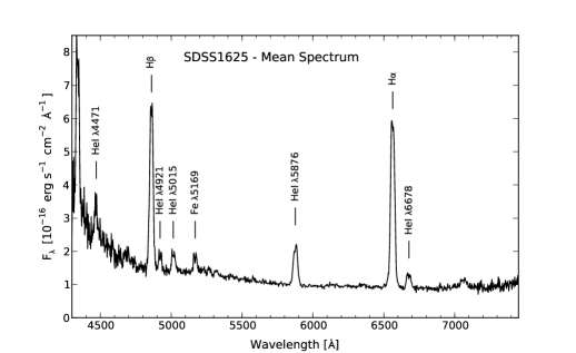
Figure 1: The mean spectrum of SDSS J162520.29+120308.7 obtained in May 2010.

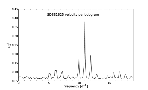
Figure 2: The periodogram for the H$\alpha$ radial velocity data of SDSS J162520.29+120308.7.

There are also several unsolved problems in our knowledge of the evolution of cataclysmic variable stars. A typical dwarf nova starts its evolution as a binary system containing a $\sim 0.6{\cal M}_{\odot}$ white dwarf and $0.2-0.5{\cal M}_{\odot}$ main sequence secondary. Initially, the orbital period is $\sim 10$ hours and this decreases due to angular momentum loss ($\dot{J}$) through magnetic braking via a magnetically constrained stellar wind from the donor star (Hameury et al. 1988, Howell et al. 1997, Kolb and Baraffe 1999, Barker and Kolb 2003). At this stage the mass-transfer rates are typically $10^{-10}-10^{-8}\leavevmode\nobreak\ \cal{M}_{\odot}\leavevmode\nobreak\ {\rm yr}$^-1. The CV evolves towards shorter periods until the secondary becomes completely convective, at which point magnetic braking greatly decreases. This happens for an orbital period of around 3 hours. Mass transfer significantly diminishes and the secondary shrinks towards its equilibrium radius, well within the Roche lobe. Abrupt termination of magnetic braking at $P_{\rm orb}\sim 3$ h produces a sharp gap, between 2 and 3 hours, in the distribution of periods of dwarf novae. The binary reawakens as a CV at $P_{\rm orb}\sim 2$ h when mass transfer recommences. It is then driven mainly by angular momentum loss due to gravitational radiation ($\dot{J}_{\rm GR}$). The orbital period continues to decrease while mass transfer stays at an almost constant level.

It is clear that observations of systems located in the period gap are very important. These systems challenge our understanding of the evolution of dwarf novae. In particular, their $q$ values are around 0.3-0.4, posing some problems for the classical TTI model (see for example the latest determination of $q$ for TU Men in Smak 2006).

In this paper we present the results of a world-wide observational campaign devoted to SDSS J162520.29+120308.7 - a newly discovered SU UMa star with an orbital period within the period gap.

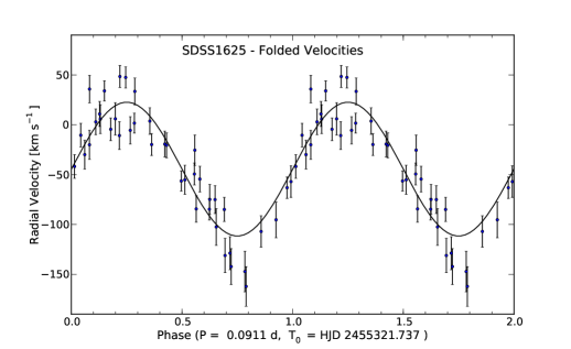
Figure 3: The H$\alpha$ radial velocities of SDSS J162520.29+120308.7 obtained in May 2010 folded on the best-fit period, with the sinusoidal fit superposed.

2 SDSS J162520.29+120308.7

SDSS J162520.29+120308.7 (hereafter SDSS J1625) was identified as a cataclysmic variable candidate by Wils et al. (2010). They pointed out that the spectrum of the star is similar to that of RZ Leo and is dominated by emission from the white dwarf and the M-dwarf companion star, with broad emission lines superimposed.

Table 1: The details of the observations collected during 2010 superoutburst of SDSS J162520.29+120308.7

Observer	Telescope	Country	No. of nights	Total time [h]	No. of frames
E. de Miguel	25 cm	Spain	16	52.395	3522
M. Otulakowska	60 cm	Poland	13	44.845	1940
A. Rutkowski	100 cm	Turkey	10	25.802	1426
R. Novak	40 cm	Czech Rep.	7	29.670	2882
G. Masi	36 cm	Italy	6	22.768	1247
M. Richmond	35 cm	USA	5	19.914	1994
B. Staels	25 cm	Belgium	4	14.187	1737
S. Lowther	25 cm	New Zealand	3	11.422	530
W. Stein	35 cm	USA	2	8.914	886
T. Ak	40 cm	Turkey	2	8.070	317
D. Boyd	35 cm	United Kingdom	2	6.266	363
R. Koff	25 cm	USA	1	5.106	545

Inspection of the Catalina Real-time Transient Survey (CRTS; Drake et al. 2009) light curve led to the discovery of modulation of the quiescent magnitude of the star with an amplitude of about 1 mag and time-scale of around 500 days.

Recent photometric data for SDSS J1625 collected by CRTS show that the star was at around 19.5 mag in 2007 and during the first half of 2008. In the second part of 2008 and the whole year 2009 it was about 1 mag brighter. In 2010 it brightened to around 18 mag.

SDSS J1625 was caught at the beginning of the outburst by CRTS in four frames taken in the interval of 5:58 - 6:35 UT on 5 July 2010. The star reached a $V$ magnitude of 13.10. About twelve hours later the first regular runs of our photometric campaign started.

Figure 4: Global light curve of the 2010 superoutburst of SDSS J162520.29+120308.7. The solid line corresponds to the parabola fit to the ’plateau’ phase.

3 Spectroscopy and Radial Velocities

We obtained pre-outburst time-series spectra in 2010 May, using the 2.4-m Hiltner telescope at MDM Observatory on Kitt Peak, Arizona, USA. The instrumentation, observing protocols, data reduction, and analysis were as described by Thorstensen et al. (2010).

The mean spectrum (Fig. 1) appears similar to the SDSS spectrum shown by Wils et al. (2010). The emission lines are all typical of dwarf novae at minimum light. H$\alpha$ has an emission equivalent width of $\sim 180$ Å, and a FWHM of nearly 1400 km s^-1. The weaker HeI lines are notably double-peaked, with the peaks separated by $\sim 1000$ km s^-1. At wavelengths $\lambda>7000$ Å, one starts to see a hint of the contribution from the M dwarf; this is much more convincingly detected in the SDSS spectrum. The sharp upturn we see at $\lambda<4700$ Åis almost certainly not as large as it appears; this is near the end of our spectral range and flux calibration is uncertain in this region. The continuum flux suggests that the $V$ magnitude averaged 18.7 for our observations; experience suggests that this should be good to $\pm 0.2$ mag or so.

The convolution function used to measure radial velocities of H$\alpha$ (see Schneider and Young, 1980 and Thorstensen et al. 2010 for details) consisted of positive and negative Gaussian functions, each with a FWHM of 275 km s^-1, separated by 1830 km s^-1. This weighted the steep sides of the line profile, outside the line core.

Fig. 2 shows the results of a period search of the resulting time series, computed using the ‘residual-gram’ method described by Thorstensen et al. (1996). Because our velocities span a range of nearly 7 h of hour angle, the daily cycle count is unambiguously determined, and a frequency near 11 cycle d^-1 is selected. The best-fit sinusoid of the form $v(t)=\gamma+K\sin[(2\pi(t-T_{0})/P]$ has $T_{0}=\hbox{HJD}\leavevmode\nobreak\ 2455321.7371(17),P_{\rm spec}=0.09111(15)\hbox{ day},\leavevmode\nobreak\ K=67(8)\hbox{ km s}^{-1}\hbox{, and }\gamma=-44(5)\hbox{ km s}^{-1}$. Fig. 3 shows the velocities folded on this best-fit period, with the sinusoidal fit superposed.

Figure 5: Superhumps observed in 2010 superoutburst of SDSS J162520.29+120308.7

4 Photometric Observations

Our observing campaign started on 5 July 2010 and ended on 11 September 2010. In total, SDSS J1625 was observed in 71 runs by 12 observers using 12 telescopes with main mirror diameters ranging from 0.25 to 1.0 meter, located in Europe, USA and New Zealand, operated mostly by members of the Center for Backyards Astrophysics (Patterson et al. 2003, 2005) and the CURVE team (Olech et al 2008, 2009). The details are given in Table 1.

The star was observed for almost 250 hours and 17389 frames were collected. ”White light” or clear filters were used. The raw images were flat-fielded and dark-subtracted by the observers. For smaller telescopes the photometry was done using commercially available software. For bigger telescopes IRAF routines were used and profile-fitting photometry was derived using the DaoPHOT/Allstar packages (Stetson 1987).

5 Global light curve

Fig. 4 shows the global light curve of SDSS J1625 in July 2010, and the beginning of August 2010. The open circle corresponds to the averaged observations of CRTS and shows that the star erupted with an amplitude of $\sim 5$ mag. After reaching a brightness of 13.1 mag at (truncated) HJD 382.76, the star started to fade with a linear trend of around 0.25 mag/day, clearly indicating that we had observed an ordinary outburst (a so-called precursor outburst), which then triggered the superoutburst. A minimum at 13.4 mag was observed near HJD 384.0, after which SDSS J1625 began to increase its brightness going into superoutburst.

A typical SU UMa star, after a rapid initial increase in brightness, enters the so-called ’plateau’ phase in which its brightness shows a roughly linear decreasing trend with a rate of $\sim 0.1-0.15$ mag per day. This phase usually lasts around 10-15 days. Some systems additionally show a small rebrightening towards the end of the plateau (see the comprehensive discussion in Kato et al. 2003 and nice example of rebrightening observed in TT Boo - Olech et al. 2004). SDSS J1625 showed a slightly different behaviour, as can be seen in Fig. 4. The plateau phase was relatively short, lasting slightly less than 8 days, and can be described by a parabola (shown as a solid line) rather than by a linear decreasing trend. It is interesting that similar behaviour was recently observed in another SU UMa star in the period gap - SDSS J162718.39+120435.0 (Shears et al. 2009).

Around HJD 392 the star entered the final decline stage and within two days it dimmed to around 17 mag. It stayed at this level for another two days, then went into a so-called echo outburst in which it reached 14.8 mag. The echo outburst finished around HJD 398 and for the following four days the star stayed at a brightness of around 17.5 mag. Further observations performed in August and September 2010 found SDSS J1625 at a brightness below 18 mag.

6 Superhumps

Fig. 5 shows the evolution of the superhumps observed during the 2010 superoutburst of SDSS J1625. At the very beginning a low-amplitude ($\sim 0.02$ mag) modulation with a period of around 0.045 days was seen. A few hours later we see the birth of ordinary superhumps. Around HJD 383.7 the first hump with a period of approximately 0.1 day and amplitude of 0.035 mag is observed. During the next two days the peak-to-peak superhump amplitude increases to almost 0.4 mag and the light modulations gain their characteristic shark-tooth shape.

Around HJD 387, the superhump amplitude starts to decrease slowly but shape remains constant for the next two days. Close to HJD 389, the superhumps start to modify their shape, showing a weak secondary hump near minimum light. These secondary humps never become strong, which is typical of systems with longer orbital periods (see Rutkowski et al 2007). Near HJD 391, the amplitude of the light variations reaches a minimum level of around 0.15 mag.

The evolution of the amplitude of superhumps is compared with that of the global light curve of the 2010 superoutburst in the two upper panels of Fig. 6.

6.1 O-C analysis

To check the value and stability of the superhump period, we performed an $O-C$ analysis for the maxima of the superhumps detected in the superoutburst light curve. In total, we determined 46 times of maxima, which are listed in Table 2 together with their cycle numbers, $E$, and $O-C$ values.

Table 2: Cycle numbers, times of maxima and $O-C$ values for superhumps observed in the 2010 superoutburst of SDSS J162520.29+120308.7. The $E=0$ epoch corresponds to the moment of highest amplitude of superhumps.

$E$	${\rm HJD_{\rm max}}$	$O-C$	$E$	${\rm HJD_{\rm max}}$	$O-C$
	$-2455000$	[day]		$-2455000$	[day]
$-$36	83.3428	$-$0.893	17	88.5329	0.064
$-$35	83.4344	$-$0.941	18	88.6283	0.056
$-$32	83.7475	$-$0.686	19	88.7210	0.019
$-$25	84.4450	$-$0.435	25	89.2995	0.034
$-$24	84.5420	$-$0.426	26	89.3915	$-$0.010
$-$23	84.6535	$-$0.267	27	89.4883	$-$0.004
$-$22	84.7530	$-$0.233	28	89.5840	$-$0.009
$-$21	84.8470	$-$0.255	29	89.6790	$-$0.021
$-$15	85.4457	$-$0.031	31	89.8673	$-$0.064
$-$14	85.5418	$-$0.032	37	90.4465	$-$0.042
$-$13	85.6420	0.010	38	90.5403	$-$0.067
$-$11	85.8380	0.047	46	91.3119	$-$0.045
$-$10	85.9380	0.087	47	91.4086	$-$0.040
$-$9	86.0350	0.095	48	91.5042	$-$0.046
$-$5	86.4238	0.137	57	92.3739	$-$0.005
$-$4	86.5185	0.122	58	92.4711	0.006
5	87.3860	0.140	59	92.5670	0.003
6	87.4798	0.116	60	92.6625	$-$0.004
7	87.5755	0.111	67	93.3413	0.052
9	87.7682	0.114	68	93.4365	0.042
10	87.8621	0.090	78	94.3870	$-$0.076
15	88.3400	0.058	100	96.4900	$-$0.213
16	88.4340	0.036	110	97.4390	$-$0.347

Figure 6: Global light curve of the 2010 superoutburst of SDSS J162520.29+120308.7 (upper panel), evolution of the amplitude of superhumps (middle panel) and $O-C$ diagram (lower panel).

The cycle numbers $E$ and times of maxima were fitted with the linear ephemeris:

$${\rm HJD}_{\rm max}=2455386.8915(3)+0.096189(10)\times E$$ (1)

indicating that the mean value of the superhump period was $P_{\rm sh}=0.096189$ day.

However, the $O-C$ diagram constructed using the above ephemeris (1) and shown in the lower panel of Fig. 6 clearly indicates the complex pattern of superhump period changes. Considered globally, it is consistent with the $ABC$ scenario recently suggested by Kato et al. (2009). In phase $A$ (negative $E$ numbers), the period is significantly longer than shown in (1); in phase $B$ ($0<E<70$), it is close to the mean value but shows a clear increasing trend; and in phase $C$ ($E>70$), the period seems to be constant and has a value shorter than the mean value.

Figure 7: $O-C$ diagram of phase A of the 2010 superoutburst of SDSS J162520.29+120308.7. The solid line corresponds to the ephemeris given by (3).

We decided to check the evolution of the superhump period by looking more closely at its behaviour in each phase. First, we fitted the following linear ephemeris to the negative $E$ numbers:

$${\rm HJD}_{\rm max}=2455386.9264(10)+0.099102(67)\times E$$ (2)

It is clear that the superhump period in this interval is longer than the mean value shown in (1). To check its stability in phase $A$, we plotted the $O-C$ diagram computed using (2). The result is shown in Fig. 7 and indicates that the superhump period was decreasing quickly at the beginning of the superoutburst. To obtain the $\dot{P}$ value, we constructed a quadratic ephemeris in the following form:

$${\rm HJD}_{\rm max}=2455386.9076(20)+0.09630(26)\times E-\\ 8.1(0.7)\cdot 10^{-5}\times E^{2}$$ (3)

The resulting value of $\dot{P}$ equals to $-1.63(14)\cdot 10^{-3}$, which is very large - one of the highest ever observed in a SU UMa system.

It is worth noting that the maxima at $E=-36$ and $E=-35$ are very uncertain due to the small amplitude of the modulation observed at that time. It is also possible that variations observed at the very beginning of the superoutburst are not connected with ordinary superhumps (this will be discussed in section 7). Omitting the first two points in the $O-C$ diagram shown in Fig. 7 does not change our conclusion concerning the very fast decrease of the superhump period during the early stage of the superoutburst.

Let’s move to phase $B$ of the superoutburst, i.e. the time interval limited by the cycle values $E$ from 0 to 70. A linear fit to the times of maxima determined in this interval is shown below:

$${\rm HJD}_{\rm max}=2455386.9006(6)+0.095942(17)\times E$$ (4)

There is a clear difference between the mean periods observed in phases $A$ and $B$ amounting to 0.003 day, i.e. about 3%.

From Fig. 7, we already know that in phase $B$ the superhump period was increasing. The second order polynomial fit to the maxima occurring during this stage is show in the following equation:

$${\rm HJD}_{\rm max}=2455386.9102(9)+0.095067(66)\times E+\\ 1.35(10)\cdot 10^{-5}\times E^{2}$$ (5)

where the quadratic term corresponds to a $\dot{P}$ value of $2.81(20)\cdot 10^{-4}$.

Fig. 8 shows the $O-C$ diagram for phase $B$ of the superoutburst constructed using (4).

Figure 8: $O-C$ diagram of phase B of the 2010 superoutburst of SDSS J162520.29+120308.7. The solid line corresponds to the ephemeris given by (5).

The amount of data collected at the end of the superoutburst (phase $C$) does not allow us to draw any conclusions about the period derivative in this interval, but the $O-C$ diagram in Fig. 6 suggests that the superhump period in phase $C$ was constant. A linear fit to the times of maxima with cycle numbers $E$ from 67 to 110 is shown below:

$${\rm HJD}_{\rm max}=2455386.9546(57)+0.09531(5)\times E$$ (6)

This indicates that, at the end of the superoutburst, the superhump period was shorter than its mean value in phase $B$. This is consistent with the scenario described recently by Kato et al. (2009).

6.2 Power spectrum analysis

The light curve from each individual run was fitted with a straight line or parabola and this fit was then subtracted from the data. This was done to remove the overall decreasing trend of the superoutburst and to bring the mean value of all runs to zero. Next, the ANOVA power spectrum was computed for the whole data set (Schwarzenberg-Czerny 1996). The resulting spectrum is shown in the upper panel of Fig. 9. It shows a clear peak at a frequency of $f=10.405(15)$ c/d with weak 1-day aliases. This frequency corresponds to a period of 0.09611(14) day which is in excellent agreement with the mean superhump period obtained in (1).

Figure 9: ANOVA statistics for the whole data set and for 1-2 day blocks.

Knowing that the superhump period was changing during the superoutburst, we decided to divide our data set into 1-2 day blocks and compute the ANOVA power spectra for each of them separately. The large amount of data collected in our campaign ensured that, even in the shortest block, the number of data points amounted to 1281. The resulting power spectra are shown in the corresponding panels of Fig. 9.

The power spectrum for HJD 383 is peculiar for two reasons. First, the main peak is located far away from the strongest frequency obtained for the whole data set. The most probable value of the frequency observed at this very early stage of the superoutburst is $f=11.13(23)$ c/d, corresponding to a period of 0.0898(18) day, which is significantly shorter that the mean period of ordinary superhumps and within the error close to the orbital period detected in spectroscopic data. The second interesting point is that a strong peak is also observed at a frequency of $2f$. This indicates that the modulation has a double wave structure which is consistent with visual inspection of the light curve for this interval.

Only one day later, at HJD 384, the situation changes completely. The main peak is located at frequency $f=9.89(15)$ c/d and there is almost no signal at $2f$. The corresponding superhump period is 0.1011(15) day i.e. much longer than its mean value obtained for the whole data set.

As we already know from the $O-C$ data analysis, during phase $A$ the superhump period was decreasing rapidly. This is fully confirmed by analysis of the next data block. For HJD 385 the ANOVA spectrum shows a very strong peak at frequency $f=10.133(130)$ c/d, again with only a very weak signal at $2f$. This frequency corresponds to a period of 0.0987(13) day. This means that during one day the period shortened by 0.0024 day (3.5 minutes) from 0.1011 to 0.0987 day.

The ANOVA spectrum for the next block (HJD 386) suggests further period decrease. The main peak is located at $f=10.42(27)$ c/d, which corresponds to a period of 0.0960(25) day.

According to the $O-C$ analysis, between HJD 386 and 387 the transition from phase $A$ to $B$ was observed, at which point the superhump amplitude reached a maximum of almost 0.4 mag.

For HJD 387 the ANOVA spectrum again shows a high peak, this time at a frequency of $f=10.441(130)$ c/d corresponding to a period of 0.0958(12) day. Within the uncertainties it is the same value as one day earlier. The $O-C$ analysis performed for the superhump maxima observed in phase $B$ showed a clear increase of the superhump period. However, the rate of this change was an order of magnitude lower than in phase $A$. Thus, it is expected that an increase in the period will not be visible in one- day block periodograms. The frequency determination in such a short interval suffers from an uncertainty of 0.1 c/d, corresponding to an uncertainty in the period determination of $\sim 0.001$ day. Taking into account the value of $\dot{P}$ determined for phase $B$, we can easily calculate that during its six days the period increased by only 0.0017 day, a value comparable with the uncertainty in the period determination for each one day interval. For this reason we abandon a detailed description of the 1-2 day block periodograms and show only a short summary of the period and power spectrum properties in Table 3.

Table 3: Values of frequencies and periods determined for the different stages of the superoutburst.

Block	$f$ [c/d]	$P$ [days]	$2f$ signal
All data	10.405(15)	0.09611(14)	medium
HJD 383	11.13(23)	0.0898(18)	very strong
HJD 384	9.89(15)	0.1011(15)	very weak
HJD 385	10.133(130)	0.0987(13)	very weak
HJD 386	10.42(27)	0.0960(25)	weak
HJD 387	10.441(130)	0.0958(12)	weak
HJD 388	10.475(150)	0.0955(14)	weak
HJD 389	10.482(150)	0.0954(14)	weak
HJD 390-391	10.397(90)	0.0962(8)	medium
HJD 329-393	10.430(96)	0.0959(8)	medium/weak

Finally, each data block was fitted with a Fourier sine series containing from 6 to 10 harmonics and this fit was used for prewhitening the original data. The ANOVA spectrum of the resulting prewhitened light curve shows no significant peaks. Thus, we conclude that the superhump signal was the one and only significant signal present during the superoutburst.

7 Quiescence

The July 2010 superoutburst of SDSS J1625 ended around HJD 394 (July 16). Following this, the star went into a so-called echo eruption which finished around HJD 398 (July 20). During the last 10 days of July, the star remained close to its quiescent magnitude.

In August and September 2010, when SDSS J1625 was at $\sim 18.5$ mag, we decided to perform two short campaigns whose main goal was to search for orbital waves. On the nights of August 1/2, 2/3, 8/9, 11/12 and 12/13 we observed the star using the 60-cm Cassegrain telescope in Ostrowik Observatory, Poland. By this time the star was poorly placed and could only be observed in the evening for 2.5 hours when it was low over the western horizon (unfortunately polluted by the lights of the neighbouring city). The resulting light curves are of poor quality (the median value of the measurement error is 0.15 mag) and visual inspection shows no clear modulation.

Figure 10: ANOVA statistics for the data collected in the period of August 1/2 - 12/13 (HJD 410 - 421).

In spite of the poor quality of the observations, we decided to compute the ANOVA statistics for this data set. The resulting periodogram is shown in Fig. 10. There are two distinct features in this plot: one group of signals centered at frequency $f_{1}=7.096(23)$ c/d and another group with the strongest signal at $f_{2}=21.196(23)$ c/d. This latter signal is interesting. It suggests that the light curve consists of a weak double humped wave with a period corresponding to $f_{2}/2$ i.e $P=0.09436(20)$ days. As the observing runs were short, the ANOVA spectrum suffers significantly from aliases. Thus we cannot exclude the possibility that the real period corresponds to one of the several aliases located at frequencies between 20 and 23 c/d.

To find the correct value of the higher frequency, we prewhitened the data with a signal characterized by the frequency of $f_{1}=7.096$ c/d. After doing this, the ANOVA power spectrum still shows the highest peak at low frequencies - this time at 8.25 c/d. This second prewhitening results in a power spectrum showing a series of peaks in a range between 22 and 27 c/d - all of them still above 3-sigma level. Due to the aliasing problem, it is difficult to determine the correct value of the frequency. It is interesting, however, that one peak is detected at frequency of $f=22.11(3)$ c/d, suggesting the possibility of the presence of double wave modulation with period of 0.0905(3) days. This value is within 2-sigma consistent both with $P_{\rm spec}=0.09111(15)$ days discussed in Sect. 3 and the period observed at very beginning of the 2010 superoutburst.

We are aware that the above analysis is speculative and based on the poor quality data. However, there are two important things. First, the power spectrum shown in Fig. 10 does not allow us to precisely determine the appropriate frequencies but indicates that there are two signals in the light curve: low frequency around 6-7 c/d and high frequency at around 21 c/d. Second, the high frequency signal might be related to double humped orbital wave.

The second campaign was performed between August 23/24 and September 11/12 when we observed SDSS J1625 on 8 nights using the 1.0-m R-C telescope at TUBITAK National Observatory, Turkey. Example light curves from four selected nights are shown in Fig. 11.

Figure 11: Quiescent light curves of SDSS J1625 obtained in August and September 2010 using a 1.0-m telescope.

Figure 12: ANOVA statistics for the data collected in the period August 23/24 - September 11/12 (HJD 432 - 451).

As TUBITAK is a mountain observatory located 2.5 km above sea level, the quality of the data was much better than for the Ostrowik runs. However, the majority of the data was collected around Full Moon which occurred on August 23.

Again we detrended the data and computed the ANOVA statistics which are shown in Fig. 12. The spectrum is quite complicated but two distinct signals (one real and one being its 1-day alias) with comparable power are observed at frequencies of $f_{1}=5.112(15)$ and $f_{2}=6.115(15)$ c/d. This low frequency modulation, corresponding to periods of 0.20 and 0.16 day respectively, is apparently visible in the light curves. It is most distinct for the night of August 26/27, when its amplitude reaches over 0.3 mag. It is interesting SDSS J1625 is not the only object showing such kind of variations (Rutkowski et al. 2010). The physical interpretation of such a modulation is still lacking.

There is no evident signal which may be interpreted as the orbital period of the binary. Prewhitening the original light curve with frequencies $f_{1}$ or $f_{2}$ produces a light curve whose power spectrum again shows some signal at frequencies around 5-6 c/d but no trace of an orbital signal.

8 Discussion

In July 2010, SDSS J1625 experienced a $\sim 5$ mag eruption lasting about 10 days. Detailed analysis of the light curve has enabled us to detect clear short-period tooth-shaped modulations whose maximum peak-to-peak amplitude reached almost 0.4 mag. These properties are characteristic of SU UMa-type dwarf novae, indicating that SDSS J1625 is a new member of this group.

The superhump period changed during the superoutburst, but as a representative value we use the mean period for phase $B$ of the superoutburst. Thus the mean superhump period of SDSS J1625 is $P_{\rm sh}=0.095942(17)$ day ($138.16\pm 0.02$ min). The orbital period of a SU UMa star is typically a few percent shorter than the superhump period, so we may expect that the orbital period of SDSS J1625 is around 130 minutes, i.e. inside the period gap.

Does our analysis reveal a candidate for the orbital period of the binary? We believe so. First of all, we refer here to the phenomenon called ”early superhumps” observed in the early stages of superoutbursts of WZ Sge type stars and first observed in the 1978 outburst of WZ Sge itself by Patterson et al. (1981). The main properties of “early superhumps” are:

• they are observed in the early stages of a superoutburst before ordinary superhumps develop. In WZ Sge stars, this early stage may last several days,

• their period is very close to the orbital period of the binary. Ishioka et al. (2002) showed that the exact period of “early superhumps” is only 0.05% shorter that the orbital period of the binary,

• they are double-wave modulations producing a power spectrum with the strongest peak at the second harmonic.

There have been several attempts at a physical interpretation of “early superhumps.” Patterson et al. (1981) suggested a “super-hot spot” model in which early humps are due to a brightened hot spot, which in turn is due to enhanced mass transfer from the secondary star during the outburst. Kato et al. (1996) favor an “early superhump” interpretation in which early humps are a premature form of true superhumps. Osaki and Meyer (2002) introduce a model where “early superhumps” are the manifestation of a tidal 2:1 resonance in the accretion disks of binary systems with extremely low mass ratios. A similar model based mainly on tidal distortion of a steady flow was suggested by Kato (2002).

There is an obvious candidate for “early superhumps” in the light curve of SDSS J1625. It is the double-wave modulation observed in the very early stage of the superoutburst (HJD 383), with a period determined to be 0.0898(18) day. The only significant difference between these humps and the “early superhumps” observed in WZ Sge systems is their duration - hours in SDSS J1625 versus days in WZ Sge stars. This property might be the reason why “early superhumps” were overlooked in ordinary SU UMa stars and observed only in low $q$ systems where they persist for much longer.

Could the period of 0.0898(18) day be associated with the orbital period of the system? It is interesting that it is consistent within the measurement errors with the modulation of 0.0904(3) day detected in the quiescent light curve of the star collected in Ostrowik and the period of 0.09111(15) day determined from spectroscopy.

There is one more test which can be done to check this hypothesis. Cataclysmic variable stars showing superhumps are known to follow the Stolz-Schoembs relation between the period excess $\epsilon$, defined as $P_{\rm sh}/P_{\rm orb}-1$, and the orbital period of the binary (Stoltz and Schoembs 1984). Fig. 13 shows this relation for over 100 dwarf novae of different types (see the figure caption for a detailed description).

Assuming that the orbital and superhump periods of SDSS J1625 are $P_{\rm orb}=0.09111(15)$ and $P_{\rm sh}=0.095942(17)$ day respectively, we calculate the period excess as $\epsilon=0.053\pm 0.002$. In Fig. 13, SDSS J1625 is plotted with a solid triangle. It is located slightly above the mean linear fit but still within the global trend, thus supporting our identification of the orbital period of the binary. Recently, an even higher value of the period excess was noted in V344 Lyr, which was observed by the Kepler mission (Still et al. 2010).

Figure 13: Dependence between period excess and orbital period of the binary for different types of cataclysmic variable. Ordinary SU UMa stars are shown with dots. Open circles represent nova-like variables and classical novae. The candidate period bouncers are plotted as open squares. The position of SDSS J1625 corresponding to the adopted orbital period of 0.09111 days is marked with the solid triangle.

Knowing the period excess and using the empirical formula given by Patterson (1998):

$$\epsilon\approx\frac{0.23q}{1+0.27q}$$ (7)

we can estimate the mass ratio $q$. In the case of SDSS J1625 it is $q\approx 0.25$. Such a high mass ratio poses a problem not only for the TTI model itself but for the explanation of “early superhumps” proposed by Osaki and Meyer (2002). Their model assumes a very low $q$ value which is needed to have sufficient matter in the disc to reach the 2:1 resonance radius. This condition is fulfilled only for $q<0.09$. For systems with $q\approx 0.25$, the outer edge of the disc not only does not reach the 2:1 resonance region but also has problems with accumulating the amount of matter at the 3:1 resonance region which, in the TTI model, is needed to produce superhumps.

Moreover, up to now the highest $q$ system which showed “early superhumps” was RZ Leo (Ishioka et al. 2001), a WZ Sge type star for which $q$ is around 0.14.

Taking into account all the above facts, maybe we should not abandon the original “super hot-spot” model proposed by Patterson et al. (1981), in which early humps are due to a brightened hot spot which in turn is due to enhanced mass transfer from the secondary. This is fully justified by the recent work of Smak (2007, 2008), which shows clear evidence for the presence of the hot spot during a superoutburst and indicates an enhanced mass transfer rate during the eruption phase (Smak 2005).

One more exceptional phenomenon observed in SDSS J1625 is the very rapid decrease of the superhump period during the early stage of the superoutburst. Looking at the model light curves of superourbursts with precursor computed both for TTI and EMT models by Schreiber et al. (2004), one can see that this early phase of superoutburst is connected with a decrease in the disc radius. In the TTI model, the disc radius decreases abruptly at the beginning and much slower during the rest of “plateau” phase. This abrupt decrease in the disc radius might be the explanation of the very high $\dot{P}$ value observed during phase $A$. In the EMT model, the decrease in disc radius at the beginning of the superoutburst is slower than in the TTI model, but still faster than in the rest of the “plateau” phase. The problem is that in both models, during phase $B$, the radius of the disc still decreases but the period of the superhumps increases.

9 Summary

1. Spectroscopic observations of SDSS J1625 performed in quiescence showed radial velocity modulations with a period of $P_{\rm spec}=0.09111(15)$ day.

2. In July 2010, SDSS J1625 experienced a superoutburst lasting for about 10 days and having an amplitude of around 5 mag. After the end of the eruption, one echo outburst was observed and the star then returned to its quiescent magnitude.

3. Superhumps were observed during almost the entire duration of the superoutburst. Their mean period in the middle phase of the superoutburst was $P_{\rm sh}=0.095942(17)$ day ($138.16\pm 0.02$ min) and their amplitude reached almost 0.4 mag.

4. The superhump period was not stable, decreasing very rapidly at a rate of $\dot{P}=-1.63(14)\cdot 10^{-3}$ at the beginning of the superoutburst and increasing at a rate of $\dot{P}=2.81(20)\cdot 10^{-4}$ in the middle phase. At the end of the superoutburst it stabilized around the value of $P_{\rm sh}=0.09531(5)$ day.

5. During the first twelve hours of the superoutburst a low-amplitude, double-wave modulation was observed whose properties are almost identical to the “early superhumps” observed in WZ Sge stars.

6. The period of the “early superhumps,” the period determined from spectroscopy, and the period of modulations observed temporarily in quiescence are the same within measurement errors, allowing us to estimate the most probable orbital period of the binary to be $P_{\rm orb}=0.09111(15)$ day ($131.20\pm 0.22$ min). This value indicates that SDSS J1625 is another dwarf nova in the period gap. Except of SDSS J1625, there are only eleven known SU UMa stars with precisely determined orbital periods with values between 2 and 3 hours.

7. From the orbital and superhump periods, we find a period excess $\epsilon=0.053\pm 0.002$, which in turn provides a mass ratio estimate of $q\approx 0.25$.

8. Such a high value of mass ratio may pose problem for some models (eg. Osaki and Meyer 2002) which explain early superhumps, and may support the idea of enhanced mass transfer and increased brightness of the hot spot during the early phase of the superoutburst.

9. Quiescent light curves of SDSS J1625 seem to consist of a lower frequency signal with strongest peaks in the range of 5-8 c/d. There is still no explanation for this kind of modulation.

- (1) Barker J., Kolb U., 2003, MNRAS, 340, 623
- (2) Drake, A.J., Djorgovski, S.G., Mahabal, A. et al, 2009, ApJ, 696, 870
- (3) Hameury J.M., King A.R., Lasota J.P., Ritter H., 1988, MNRAS, 231, 535
- (4) Hellier, C., 2001, Cataclysmic Variable Stars - How and Why they Vary, Springer Berlin
- (5) Hirose, M., Osaki, Y., 1990, PASJ, 42, 135
- (6) Howell S.B., Rappaport S., Politano M., 1997, MNRAS, 287, 929
- (7) Ishioka, R., Kato, T., Uemura, M. et al., 2001, PASJ, 53. 905
- (8) Ishioka, R., Uemura, M., Matsumoto, K. et al., 2002, A&A, 381, L41
- (9) Kato, T., Nogami, D. Baba, H., Matsumoto, K., Arimoto, J., Tanabe, K., Ishikawa, K., 1996, PASJ, 48, 21
- (10) Kato, T., 2002, PASJ, 54, L11
- (11) Kato, T., Nogami, D., Moilanen, M., Yamaoka, H., 2003, PASJ, 55, 989
- (12) Kato, T., Imada, A., Uemura, M., et al. 2009, PASJ 61, S395
- (13) Kolb U., Baraffe I., 1999, MNRAS, 309, 1034
- (14) Lubow, S.H., 1991, ApJ, 381, 259
- (15) Olech, A., Cook, L.M., Zloczewski, K., Mularczyk, K., Kedzierski, P., Udalski, A., Wisniewski, M., 2004, Acta Astron., 54, 233
- (16) Olech, A., Wisniewski, M., Zloczewski, K., Cook, L. M., Mularczyk, K., Kedzierski, P., 2008, Acta Astron., 58, 131
- (17) Olech, A., Rutkowski, A., Schwarzenberg-Czerny, A., 2009, MNRAS, 399, 465
- (18) Osaki, Y., 1989, PASJ, 41, 1005
- (19) Osaki, Y., 1996, PASP, 108, 39
- (20) Osaki, Y., 2005, Proceedings of the Japan Academy, Ser. B: Physical and Biological Sciences, Vol. 81, p. 291
- (21) Osaki, Y., Meyer, F., 2002, A&A, 383, 574
- (22) Patterson, J., McGraw, J.T., Coleman, L., Africano, J.L., 1981, ApJ, 248, 1067
- (23) Patterson, J., 1998, PASP, 110, 1132
- (24) Patterson, J., Thorstensen, J.R., Kemp, J. et al, 2003, 115, 1308
- (25) Patterson, J., Kemp, J., Harvey, D.A. et al., 2005, 117, 1204
- (26) Rutkowski, A., Olech, A., Mularczyk, K., Boyd, D., Koff, R., Wisniewski, M., 2007, Acta Astron., 57, 267
- (27) Rutkowski, A., Olech, A., Poleski, R., Sobolewska, M., Kankiewicz, P., Ak, T., Boyd, D., 2010, Acta Astron, 60, 337
- (28) Schneider, D.P., Young, P., ApJ, 238, 946
- (29) Schreiber, M.R., Hameury, J.-M., Lasota, J.-P., 2004, A&A, 427, 621
- (30) Schreiber, M.R., Lasota, J.-P., 2007, A&A, 473, 897
- (31) Schwarzenberg-Czerny A., 1996, ApJ Letters, 460, L107
- (32) Shears, J., Brady, S., Gansicke, B., Krajci, T., Miller, I., Ogmen, Y., Pietz, J., Staels, B., 2009, JBAA, 119, 144
- (33) Smak, J., Waagen, E., 2004, Acta Astron., 54, 433
- (34) Smak, J., 2005, Acta Astron., 55, 315
- (35) Smak, J., 2006, Acta Astron., 56, 277
- (36) Smak, J., 2007, Acta Astron., 57, 87
- (37) Smak, J., 2008, Acta Astron., 58, 65
- (38) Smak, J., 2009, Acta Astron., 59, 103
- (39) Stetson P.B., 1987, PASP, 99, 191
- (40) Still, M., Howell, S.B., Wood, M.A., Cannizzo, J.K., Smale, A.P., 2010, ApJ Letters, 717, L113
- (41) Stolz B., Schoembs R., 1984, A&A, 132, 187
- (42) Thorstensen, J. R., Patterson, J. O., Shambrook, A., & Thomas, G. 1996, PASP, 108, 73
- (43) Thorstensen, J. R., Peters, C. S., & Skinner, J. N. 2010, PASP, 122, 1285
- (44) Warner, B., 1995, Cataclysmic Variable Stars
- (45) Whitehurst, R., 1988, MNRAS, 232, 35
- (46) Wils, P., Gansicke, B.T., Drake, A.J., Southworth, J., 2010, MNRAS, 402, 436