$SL(2,\mathbb{R})$ Chern-Simons, Liouville,
and Gauge Theory on Duality Walls

Abstract

We propose an equivalence of the partition functions of two different 3d gauge theories. On one side of the correspondence we consider the partition function of 3d $SL(2,\mathbb{R})$ Chern-Simons theory on a 3-manifold, obtained as a punctured Riemann surface times an interval. On the other side we have a partition function of a 3d $\mathcal{N}=2$ superconformal field theory on $S^{3}$, which is realized as a duality domain wall in a 4d gauge theory on $S^{4}$. We sketch the proof of this conjecture using connections with quantum Liouville theory and quantum Teichmüller theory, and study in detail the example of the once-punctured torus. Motivated by these results we advocate a direct Chern-Simons interpretation of the ingredients of (a generalization of) the Alday-Gaiotto-Tachikawa relation. We also comment on M5-brane realizations as well as on possible generalizations of our proposals.

1 Introduction

Over the past decades the notion of duality has played a key role in the study of gauge theories and string theories. The word duality traditionally refers to an equivalence of two different physical theories, but there are important examples of “duality” which do not fall into this category: a pair of two theories, although different as physical theories, share certain common quantities, which have different physical meanings and can be computed by completely different methods in the two theories. In other words, this is a duality as an equivalence of two quantities (e.g. the partition functions) or subsectors (e.g. ground state Hilbert spaces) of the two theories, as opposed to an equivalence of the full theories themselves. This extended notion of duality, although limited in its power and scope, is much more general, and provides a useful bridge between theories which are unrelated otherwise. A good example for this is the recently discovered Alday-Gaiotto-Tachikawa (AGT) relation, which claims an equivalence of the instanton partition functions of 4d $\mathcal{N}=2$ $SU(2)$ superconformal field theories on $S^{4}$ and conformal blocks of 2d Liouville theory on Riemann surfaces [1].

In this paper, we initiate a program to connect two different 3d gauge theories — one is a (bosonic) 3d $SL(2,\mathbb{R})$ Chern-Simons theory and another is a 3d $\mathcal{N}=2$ superconformal field theory. This provides yet another example of the generalized duality in the sense mentioned above. In particular, we propose an equivalence of the partition function of the two theories. This is schematically written as

$$Z_{\textrm{3d $SL(2,\mathbb{R})$ CS}}=Z_{\textrm{3d $\mathcal{N}=2$ theory}}.$$ (1.1)

More precise formulation of this statement, as well as explicit examples, will be given below.

We will arrive at the relation (1.1) by a chain of connections with quantum Teichmüller theory and quantum Liouville theory, each step interesting in its own right. For example, in one step we will encounter a new state sum model for $SL(2,\mathbb{R})$ Chern-Simons theory defined from quantum Teichmüller theory. Assuming several conjectures in the literature, this almost gives a proof of the relation (1.1). This will also clarify the connection between our proposal and the AGT conjecture and its generalization [2]. From this viewpoint the relation (1.1) should be thought of as a (3+3) version of AGT relation, which divides 6 into (4+2) (see the cautionary remarks in section 3, however). In fact, this understanding leads to an interesting question of reformulating everything we know about the AGT correspondence (and its generalization) in the language of $SL(2,\mathbb{R})$ Chern-Simons theory. We will provide partial answer to this problem in this paper. In particular, the underlying reason for our correspondence is that there is a natural identification of the Hilbert spaces of all the four theories, which identification one might be tempted to call “Gauge/Liouville/Teichmüller/Chern-Simons correspondence”

$$\mathcal{H}_{\textrm{4d gauge}}(S^{3})=\mathcal{H}_{\textrm{Teichm\"{u}ller}}(\Sigma)=\mathcal{H}_{\rm Liouville}(\Sigma)=\mathcal{H}_{\textrm{Chern-Simons}}(\Sigma).$$ (1.2)

The rest of this paper is organized as follows. In section 2 we give more precise formulation of our conjectures. In section 3 we outline the logic used in deriving the conjecture. Section 4 discuss the example of once-punctured torus in detail. In section 5 we briefly comment on generalizations to higher rank gauge groups. In section 6 we discuss several open problems which we hope will be answered in the future. In appendices we collect results useful for the understanding of this paper. In particular, readers are encouraged to consult appendix A for the construction of the Hilbert space in quantum Teichmüller theory.

2 Summary of Our Proposal

In order to give a more precise formulation of (1.1), let us explain the necessary ingredients in detail. On the left hand side of the correspondence we consider a Chern-Simons theory with a non-compact gauge group $SL(2,\mathbb{R})$ . This theory has a Lagrangian

$$S=\int_{M}\frac{k}{4\pi}\textrm{Tr}\left(\mathcal{A}\wedge d\mathcal{A}+\frac{2}{3}\mathcal{A}\wedge\mathcal{A}\wedge\mathcal{A}\right),$$ (2.1)

where $\mathcal{A}$ is a $SL(2,\mathbb{R})$-valued connection, $M$ is a 3-manifold, and $k$ is the level of the Chern-Simons theory. The partition function is defined by

$$Z(M)=\int\!\mathcal{D}\!\mathcal{A}\,\,e^{iS}.$$ (2.2)

When the 3-manifold $M$ has boundaries, we need to supplement this definition with the choice of boundary conditions.

For the purpose of this paper our 3-manifold $M$ will be defined from the following three ingredients. First, we choose a Riemann surface $\Sigma_{g,h}$, where $g$ ($h$) denotes the genus (the number of holes). $\Sigma_{g,h}$ is hereafter often going to be written $\Sigma$ for notational simplicity. We assume that $\Sigma$ is hyperbolic, i.e., satisfies

$$2g-2+h>0.$$ (2.3)

Another technical subtlety here is that the holes in general are assumed to be of finite size, i.e. each puncture $p_{i}$ is associated with a number $m_{i}$, representing the size of the puncture.

Second, we choose two boundary conditions on the Riemann surface $\Sigma$. As we will see later, for boundary conditions we first need to choose a pants decomposition of $\Sigma$ and then a set of $3g-3+h$ integers, which we collectively write $l$ (and $l^{\prime}$ for another). We choose the same pants decomposition for the two boundary conditions $l$ and $l^{\prime}$. $l$ and $l^{\prime}$ will be the length coordinates, half of the length-twist coordinates of the Teichmüller space of $\Sigma$ (see appendix A.2). Recall that the Teichmüller space $\mathcal{T}_{g,h}$ of a Riemann surface $\Sigma_{g,h}$ is the space of complex structure deformations of $\Sigma_{g,h}$, divided by the identity component of the diffeomorphisms of $\Sigma_{g,h}$:

$$\mathcal{T}_{g,h}=\frac{\{\textrm{complex structure on }\Sigma_{g,h}\}}{\mathrm{Diff}_{0}(\Sigma_{g,h})}.$$ (2.4)

This is a Kähler manifold of complex dimension

$$\mathrm{dim}_{\mathbb{C}}\,\mathcal{T}_{g,h}=3g-3+h.$$ (2.5)

Third, we fix an element $\varphi$ of the mapping class group $\Gamma_{g,h}$ of $\Sigma$, which is defined by

$$\Gamma_{g,h}=\frac{\mathrm{Diff}(\Sigma_{g,h})}{\mathrm{Diff_{0}}(\Sigma_{g,h})}.$$ (2.6)

This acts on $\mathcal{T}_{g,h}$, and the quotient $\mathcal{M}_{g,h}=\mathcal{T}_{g,h}/\Gamma_{g,h}$ is the moduli space of the Riemann surface.

Our 3-manifold $M_{\Sigma,(l,l^{\prime}),\varphi}$ is then defined to be $\Sigma\times I$, where $I=[0,1]$ is an interval and the boundary conditions at $\partial M=\Sigma\times\{0\}\cup\Sigma\times\{1\}$ are determined by $l$ and $\varphi(l^{\prime})$ . The Chern-Simons partition function we have in (1.1) is defined on this manifold. When we make the dependence explicit, we have

$$Z_{CS}\left[M_{\Sigma,(l,l^{\prime}),\varphi}\right](m,k),$$ (2.7)

where $m$ collectively refers to a set of parameters $\{m_{i}\}$.

Let us next describe the other side of the correspondence. On this side we regard the Riemann surface $\Sigma$ as the so-called Gaiotto curve [3]. In other words we consider 4d $\mathcal{N}=2$ generalized quiver superconformal field theories obtained by compactifying 6d $(2,0)$ theory (theories on multiple M5-branes) on $\Sigma$. For the most of this paper we consider the case of two M5-branes, i.e. the gauge group of the 4d theory is $SU(2)$. We will briefly comment on the higher rank generalization in section 5.

In Gaiotto’s construction, the moduli space of the Riemann surface $\Sigma$ is interpreted as the space of marginal deformations of 4d superconformal field theory, and the mapping class group of the Riemann surface is identified with the S-duality group of the 4d $\mathcal{N}=2$ theory. This in particular means that we can regard $\varphi$ as a symmetry of the 4d $\mathcal{N}=2$ theory, and the physics at value of complexified gauge coupling $\tau$ is equivalent to the physics at $\varphi(\tau)$. Here $\tau$ is defined from the gauge coupling constant $g$ and the theta-angle $\theta$ by

$$\tau=\frac{4\pi i}{g^{2}}+\frac{\theta}{2\pi}.$$ (2.8)

The 4d theory is in general strongly coupled – only at the boundary of the moduli space where the Riemann surface degenerates (this is specified by a choice of pants decomposition) do we have a Lagrangian description of the 4d theory. Finally, the hole parameters $m_{i}$ in 2d are interpreted as the mass parameters of the 4d theory,

The 3d $\mathcal{N}=2$ theory we are interested in is realized as a theory on the 1/2 BPS duality domain wall inside this 4d $\mathcal{N}=2$ theory. To define this, let us consider $\mathbb{R}^{3,1}$, and divide one of the spatial directions (say, $x^{3}$) into two parts, $x^{3}>0$ and $x^{3}<0$. On one side $x^{3}>0$ we consider 4d theory with complexified gauge coupling $\tau$, and on the other ($x^{3}<0$) we consider the same theory with different values of the complexified gauge coupling: we take the value to be $\varphi(\tau)$, where as above $\varphi$ is an element of the duality group. The complexified gauge coupling $\tau$ then has a non-trivial profile near $x^{3}=0$ (Janus solution), and we in particular consider a profile preserving half of the supersymmetries. We can make the value of $\tau$ constant in the whole $\mathbb{R}^{3,1}$ by taking an S-duality in $x^{3}<0$, and all the effect of $\varphi$ is localized around $x^{3}=0$ . Since our 4d theory is conformal we can squeeze everything into $x^{3}=0$ and we have a 3d domain wall at $x^{3}=0$. This domain wall is often called a “duality wall” since it is specified by an element $\varphi$ of the 4d duality group. It is the 3d $\mathcal{N}=2$ theory (1/2 BPS in 4d $\mathcal{N}=2$ theory) on this duality domain wall that we study in this paper. We are going to call the 4d theory the mother theory, and the 3d theory the daughter theory. In the following we will denote the daughter theory by $T[SU(2);\varphi;m]$ .

In the above description of the 3d theory, 3d theory on the wall couples to the bulk 4d theory. However, as we will see later in examples, 3d theories themselves can be defined purely in 3d; the bulk gauge fields couple with the 3d theory by gauging the global symmetries in 3d. The 3d theory has global symmetry $SU(2)\times SU(2)$ , and correspondingly the theory has two parameters $a$ and $a^{\prime}$, each representing either the mass parameter or the Fayet-Iliopoulos (FI) parameter. These parameters are defined by coupling 3d theory to a background gauge fields.

It should be emphasized that our daughter theories can be defined purely in 3d, without the coupling to the bulk 4d theory. The reason we refer to 4d gauge theories is twofold: first, very little is known about these 3d theories themselves (except for the case of $\Sigma_{1,1}$ which will be discussed later). Second, our definition of 3d theory as a theory of domain walls in 4d will be crucial when we discuss the connection with the AGT relation.

Let us make one cautionary remark here. This 3d theory we just described often (but not always) contains gauge fields with Chern-Simons terms with compact gauge group $SU(2)$. This Chern-Simons term should not be confused with the pure bosonic $SL(2,\mathbb{R})$ Chern-Simons theory in the other 3d. For the most of the following discussion the word Chern-Simons often refers to the latter theory.

Finally, the right hand side of (1.1) is defined as a partition function of the 3d theory on a $S^{3}$, whose metric is deformed from the standard metric by a single parameter $b$. In this paper we call this 3-sphere a deformed 3-sphere, and denote it by $S^{3}_{b}$ . The deformed 3-sphere $S^{3}_{b}$ preserves $U(1)\times U(1)$ isometry of the $SO(4)=SU(2)\times SU(2)$ isometry of the standard $S^{3}$, and can be defined by an equation

$$b^{2}(dx_{1}^{2}+dx_{2}^{2})+b^{-2}(dx_{3}^{2}+dx_{4}^{2})=1.$$ (2.9)

When set to $b=1$, this reduces to the $S^{3}$ with the standard metric.

Now we can define the partition function of our theory on $S^{3}_{b}$

$$Z_{\left[T[SU(2);\varphi;m]\right]}\left[S^{3}_{b}\right]\left(a,a^{\prime}\right).$$ (2.10)

The (1.1) is an equivalence of two expressions given so far, i.e.,

$$Z_{\left[T[SU(2);\varphi;m]\right]}\left[S^{3}_{b}\right]\left(a,a^{\prime}\right)=Z_{CS}\left[M_{\Sigma,(l,l^{\prime}),\varphi}\right](m,k),$$ (2.11)

under the parameter identification

$$a=l,\quad a^{\prime}=l^{\prime},$$ (2.12)

and

$$\hbar:=\frac{4\pi}{k+2}=2\pi b^{2}.$$ (2.13)

In the discussion above we have chosen a 3-manifold $M_{\Sigma,l,\varphi}$ with two boundaries. Instead, we can choose to close up the boundaries by identifying the two boundary Riemann surfaces. We then have the mapping torus $M_{\Sigma,\varphi}$, which is defined to be a $\Sigma$-bundle over $S^{1}$, with an action of $\varphi$ when we go around $S^{1}$:

$$M_{\Sigma,\varphi}=(\Sigma\times\left[0,1\right])/\{(x,0)\sim(\varphi(x),1)\}.$$ (2.14)

There is a corresponding operation on the gauge theory side. Our gauge theory, $T[SU(2);\varphi;m]$, is defined by a linear quiver with two ends, and we can identify the two ends of the quiver to make it into a circular quiver (see Figure 5 (b) and (c)). The dependence of the partition function on $a$ and $a^{\prime}$ are drop out (these parameters are going to be integrated out), and (2.11) becomes a statement

$$Z_{CS}\left[M_{\Sigma,\varphi}\right](m,k)=Z_{T[SU(2);\varphi;m]}\left[S^{3}_{b}\right].$$ (2.15)

The parameter identification (2.13) is highly non-trivial. First, the value of $k$ is quantized while $b$ is a continuous parameter. This suggests that on the Chern-Simons side it is natural to perform an analytic continue the gauge group into the complexified gauge group $SL(2,\mathbb{C})$, whose action reads

$$\!\!S=\frac{t}{8\pi}\!\int\!\textrm{Tr}\left(\mathcal{A}\wedge d\mathcal{A}+\frac{2}{3}\mathcal{A}\wedge\mathcal{A}\wedge\mathcal{A}\right)+\frac{\bar{t}}{8\pi}\!\int\!\textrm{Tr}\left(\bar{\mathcal{A}}\wedge d\bar{\mathcal{A}}+\frac{2}{3}\bar{\mathcal{A}}\wedge\bar{\mathcal{A}}\wedge\bar{\mathcal{A}}\right)\!,\,$$ (2.16)

where $\mathcal{A}$ ($\bar{\mathcal{A}}$) are holomorphic (antiholomorphic) connection and we write $t=k+s,\bar{t}=k-s$. Consistency requires that $k$ is an integer as usual, but $s$ is not, and can either be real or pure imaginary [5]. Such an analytic continuation is natural also from the viewpoint of 6d (2,0) theory, since a triplet of Higgs scalars coming from the dimensional reduction of a 6d vector multiplet complexifies the gauge field (cf. [6]).

Second, there is a symmetry

$$b\leftrightarrow b^{-1}.$$ (2.17)

In 3d gauge theory, this is a geometrically corresponds to an exchange of the 2 $U(1)$ isometries (exchanging $(x_{1},x_{2})$ with $(x_{3},x_{4})$ in (2.9)). This will appear as the modular duality of Liouville theory [7], or more mathematically as an identity (B.6) of quantum dilogarithm [8], or as a modular double of a quantum group [9]. This should be interpreted as an S-duality of the $SL(2,\mathbb{R})$ Chern-Simons theory. We will make further comments on this in the last section.

3 Basic Idea

In this subsection we give an evidence for the proposal above. In short, we use quantum Liouville theory and quantum Teichmüller theory as a bridge between the two 3d theories (see Figure 1). This is by no means a complete proof of our proposal, since we need to invoke several conjectures existing in the literature, including the AGT relation, which are assumed in this paper. Nevertheless the following argument is a good starting point for the complete proof of our proposal, and moreover provides a coherent perspective unifying all the theories discussed in this paper. Of course, the physical reason for such a unification should be explained from the existence of the mysterious 6d $(2,0)$ theory.

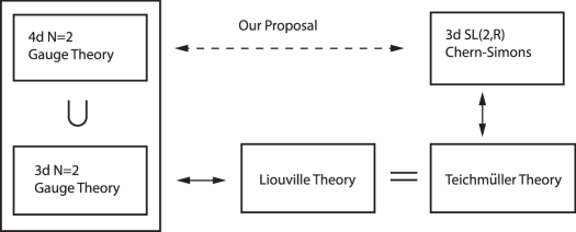
Figure 1: The flow of logic of this section (and the paper).

In the following we explain each of the steps in Figure 1 in some more detail.

3.1 Step 1: Gauge to Liouville

Let us begin with the right hand side of (2.11), (2.15). As we explained, the daughter 3d $\mathcal{N}=2$ is defined as a theory on the duality domain wall inside the mother 4d $\mathcal{N}=2$ superconformal field theory, so let us begin with this mother theory. When this theory is placed on a compact manifold $S^{4}$, its partition function can be computed by localization [10], and is given by

$$Z_{\rm 4d}[S^{4}](q;m;\epsilon_{1},\epsilon_{2})=\int\!da\,\,\nu(a)\,\overline{Z_{\rm Nek}(q;a,m;\epsilon_{1},\epsilon_{2})}Z_{\rm Nek}(q;a,m;\epsilon_{1},\epsilon_{2}),$$ (3.1)

where $a$ is the Coulomb branch parameter, $m$ mass parameters, $q:=e^{2\pi i\tau}$ and $Z_{\rm Nek}$ is the instanton partition function studied by Nekrasov [11], with $\epsilon_{1},\epsilon_{2}$ being the parameters of $\Omega$-deformation. These two parameters can be traded for the two parameters $b$ and $\hbar$, defined by

$$\epsilon_{1}=\hbar b,\quad\epsilon_{2}=\hbar/b.$$ (3.2)

The overall parameter $\hbar$ is identified with the inverse radius of $S^{4}$, and in the following we are going to set $\hbar=1$. Also, in Pestun’s computation we actually have $b=1$, although it is natural to conjecture and existence of a 1-parameter family of manifold $S^{4}_{b}$ which reproduce (3.1) with $b\neq 1$. In the following we are going to deal with the right hand side of (3.1) with $b\neq 1$. In the computation of localization, the two factors $Z_{\rm Nek}$ and $\overline{Z}_{\rm Nek}$ are the contributions from the fixed points at the north and the south pole, respectively, and the measure $\nu(a)$ contains classical as well as one-loop contributions.

AGT relation [1] states the equivalence of this partition function with a correlator of the Liouville theory on $\Sigma$. To fix notations, let us remind ourselves that Liouville theory is defined by an action

$$S=\int d^{2}z\left(\partial\phi\bar{\partial}\phi+\pi\mu e^{2b\phi}\right).$$ (3.3)

This theory has central charge $c=1+6Q^{2}$, where we defined $Q=b+b^{-1}$. The primary operators are given by $V_{\alpha}=e^{\alpha\phi}$, which has conformal dimension

$$\Delta(\alpha)=\alpha(Q-\alpha).$$ (3.4)

Let us consider a correlator of these vertex operators. When we specify the pants decomposition $\sigma$ of the Riemann surface, the correlator factorizes into the product of holomorphic and anti-holomorphic conformal blocks $\mathcal{F}^{\sigma}_{\alpha,E}$

$$\Big{\langle}\prod_{i}V_{m_{i}}\Big{\rangle}_{\Sigma}=\int d\alpha\,\nu(\alpha)\,\overline{\mathcal{F}_{\alpha,E}({q})}\mathcal{F}_{\alpha,E}(q),$$ (3.5)

where $\alpha$ and $E$ denotes (the set of) internal and external momenta, respectively, and $q$ ($\bar{q}$) denotes the complex structure (and its conjugate) of $\Sigma$. We include the DOZZ 3-point function [12, 13] in the measure $\nu(\alpha)$, which takes the form

$$\nu(\alpha)=\prod_{i}\sin(\pi\alpha_{i}b)\sin(\pi\alpha_{i}/b).$$ (3.6)

Now the first claim of AGT is that Nekrasov partition function of the 4d $\mathcal{N}=2$ theory coincides with the conformal block of Liouville theory, under the parameter identification

$$\alpha=\frac{Q}{2}+a,\quad E=m.$$ (3.7)

The second claim is that the measure $\nu(a)$ from the classical and 1-loop partition function coincides with the product of DOZZ 3-point functions. These yield the celebrated AGT relation, which claims the equivalence of a correlator with the 4d partition function

$$Z_{\rm 4d}[S^{4}]=\Big{\langle}\prod_{i}V_{m_{i}}\Big{\rangle}_{\Sigma}.$$ (3.8)

4d gauge theories contain a rich class of BPS defect operators. For example, Pestun’s localization applies to the case with a Wilson line operator. In general, we can consider the VEV of a 1/2 BPS loop operator $L$ in 4d $\mathcal{N}=2$ theory. The counterpart of this in Liouville theory is the Verlinde loop operator $\mathcal{L}$ [14]. There is a one-to-one correspondence between a classification of charges of loop operators and the Dehn-Thurston data of the non-self-intersecting curves on the Riemann surface [15]. Moreover, as shown in [16, 17], the VEV of the line operator in spin $j$ representation is equal to the Liouville correlator with a Liouville loop operator $\mathcal{H}$ corresponding to a degenerate field $\Phi_{1,2j+1}$ inserted:

$$\Big{\langle}L\Big{\rangle}_{S^{4}}=\Bigg{\langle}\left(\prod_{i}V_{m_{i}}\right)\mathcal{L}\Bigg{\rangle}_{\Sigma}.$$ (3.9)

In this paper we consider yet another type of operators in 4d gauge theories: the domain wall operators. As already discussed in the previous subsection, we are going to consider a 1/2 BPS domain wall. We introduced this as a domain wall $\mathbb{R}^{3}$ in $\mathbb{R}^{4}$, but in order to make contact with the story in this subsection we here consider a 1/2 BPS duality domain wall placed on equator $S^{3}$ of $S^{4}$. Summarizing, we have 4d theory on $S^{4}$, together with a duality wall on the equator, and our 3d $\mathcal{N}=2$ theory lives on this equator $S^{3}$ (Figure 2).

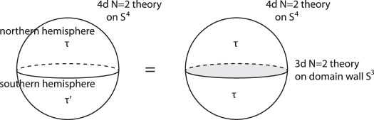
Figure 2: Our 3d $\mathcal{N}=2$ theory is realized as a duality domain wall $S^{3}$ inside $S^{4}$, where the mother 4d $\mathcal{N}=2$ theory lives. On the left figure, the complexified gauge coupling of the mother 4d theory in the northern (southern) hemisphere is given by $\tau$ ($\tau^{\prime}$), where $\tau^{\prime}$ is related to $\tau$ by an action of the S-duality group element $\varphi$: $\tau^{\prime}=\varphi(\tau)$. Instead, we can take S-duality in the southern hemisphere to make the complexified gauge coupling $\tau$ in the whole $S^{4}$, but then we have a non-trivial 3d theory on the equator $S^{3}$.

The domain wall preservers the symmetry used for localization, and hence the partition function of the 4d theory is again computed by localization. Precise computation of the 1-loop determinant can be subtle, but [2] proposed the following expression

$$Z_{\rm 4d+3d}(S^{4})=\int dada^{\prime}\,\nu(a)\nu(a^{\prime})\,\overline{Z_{\rm Nek}(a,m)}Z_{\rm 3d}(a,a^{\prime},m)Z_{\rm Nek}(a^{\prime},m),$$ (3.10)

where the measure $\nu(a)$ is the same expression as before. $Z_{\rm 3d}(a,a^{\prime},m)$ is the partition function of 3d theory $T[SU(2);\varphi;m]$ on $S^{3}$, with $a$ and $a^{\prime}$ being either the mass parameter or the FI parameter of the 3d theory. The 3d theory couples to the bulk by gauging the global symmetry. $Z_{\rm Nek}$ and $\overline{Z_{\rm Nek}}$ are contributions from the fixed points at the north pole and the south pole, respectively, and $Z_{\rm 3d}[a,a^{\prime}]$ is the contribution from the domain wall.

Now the natural question is whether there is a counterpart of this story in the Liouville side. This has been analyzed in [2], and the answer is that it corresponds to an insertion of a non-degenerate field, which changes (3.5) into

$$\int d\alpha\,\nu(\alpha)\,\overline{\mathcal{F}_{\alpha,E}(q)}\mathcal{F}_{\alpha,E}(q^{\prime}),$$ (3.11)

where $q^{\prime}=e^{2\pi i\tau^{\prime}}$ with $\tau^{\prime}=\varphi(\tau)$. Now the action of an element $\varphi$ of the mapping class on the conformal block can be represented by an integral kernel

$$\mathcal{F}_{\alpha,E}(q^{\prime})=\int d\alpha^{\prime}\nu(\alpha^{\prime})\,(\mathsf{\varphi})_{\alpha,\alpha^{\prime}}\,\mathcal{F}_{\alpha^{\prime},E}(q).$$ (3.12)

This is an analog of the modular transformation of characters in rational conformal field theory (CFT) — here we have an integral instead of a sum since our CFT, Liouville, is irrational. For torus without punctures the kernel $\mathsf{\varphi}$ is indeed determined from the modular transformation of characters.

Substituting (3.12) into (3.11), we have

$$\int d\alpha d\alpha^{\prime}\,\nu(\alpha)\nu(\alpha^{\prime})\,\mathcal{F}_{\alpha,E}(q)\varphi_{\alpha,\alpha^{\prime}}\mathcal{F}_{\alpha,E}(q).$$ (3.13)

Comparing (3.10) and (3.13), we conclude that the two expressions are the same if we identify the partition function of the 3d domain wall theory with an integral kernel representing $\varphi$ [2, 18]:

$$Z_{3d}[a,a^{\prime}]=\varphi_{\alpha,\alpha^{\prime}}.$$ (3.14)

where the parameter identifications are given by

$$a=\alpha,\quad a^{\prime}=\alpha^{\prime}.$$ (3.15)

In section 4, we review existing checks and provide further evidence for this conjecture (3.14). The relation (3.14) will be assumed for the discussion of the rest of this paper. and we call the equivalence of (3.10) and (3.13) the “generalized AGT relation”.

3.2 Step 2: Liouville to Teichmüller

Now that we obtained the expression in Liouville theory, the next step is to rewrite everything in Teichmüller theory.

To explain why this is possible, let us begin with the classical theory. The uniformization theorem states that for each element of the Teichmüller space there exists a unique constant negative curvature metric of the form

$$ds^{2}=e^{2b\phi}dzd\bar{z}.$$ (3.16)

This metric has a constant negative curvature iff $\phi$ satisfies the Liouville equation

$$\partial\bar{\partial}\phi=2\pi\mu be^{2b\phi},$$ (3.17)

which coincides with the equation of motion for the Liouville action (3.3). This is the classical equivalence between Liouville and Teichmüller theory.

There is a quantum counterpart of this equivalence. When we write the two Hilbert spaces for the two theories on a Riemann surface $\Sigma$ by $\mathcal{H}_{L}(\Sigma),\mathcal{H}_{T}(\Sigma)$, we have

$$\mathcal{H}_{L}(\Sigma)=\mathcal{H}_{T}(\Sigma),$$ (3.18)

where the equality is meant to include the equality of the mapping class group action as well. This was originally conjectured by a seminal paper by H. Verlinde [19] in the 80’s. The explicit construction of quantum Teichmüller theory was given in the mid 90’s [20, 21], and more recently there are important contributions [22, 23] which almost proves the equivalence of the two theories. See also [24], which established a direct correspondence between quantum discrete Liouville theory and quantum Teichmüller theory.

Quantum Teichmüller theory is a framework to construct the Hilbert space $\mathcal{H}_{T}(\Sigma)$. The precise definition of the Hilbert space of quantum Teichmüller space will be given in appendix A, and we will give concrete discussion in section 4. Here we summarize the minimal ingredients needed for the purpose of this section.

It is important for our purposes that there are several natural different bases in $\mathcal{H}_{T}(\Sigma)$. One basis is the holomorphic basis $|\tau\rangle$, where $\tau$ is a holomorphic coordinate parametrizing the complex structure of $\Sigma$. This arises from the Kähler quantization of the Teichmüller space.

Another is the length basis $|l\rangle$. This is obtained when we specify a pants decomposition $\sigma$, and where $l=\{l_{i}\}$ are eigenvalues of the geodesic length operators and takes values in $\mathbb{R}_{>0}$. In the language of Liouville theory, these length operators are precisely the Verlinde loop operators [17] ($\mathcal{L}$ in (3.9)), and the basis $|l\rangle$ is the eigenspace of maximally commuting set of Verlinde loop operators determined by the pants decomposition. The important property of the basis is that they span a complete basis in $\mathcal{H}_{\Sigma}$ [25]

$$\langle l|l^{\prime}\rangle=\nu(l)^{-1}\delta(l-l^{\prime}),\quad\int dl\,\nu(l)\,|l\rangle\langle l|=1,$$ (3.19)

where $\nu(l)$ is the same function as defined in (3.6).

What we would like to do from now on is to rewrite the expressions (3.5), (3.13) in the language of quantum Teichmüller theory. The crucial observation for this is that the conformal block of the Liouville theory can be identified with the overlap of holomorphic basis and length basis in quantum Teichmüller theory [22]:

$$\mathcal{F}_{\alpha,E}(q)=\langle l|q\rangle,$$ (3.20)

where the length parameters $l$ are identified with the Liouville momentum $\alpha$

$$\alpha=l,$$ (3.21)

and the puncture parameters $m$, corresponding to external momenta $E$, are suppressed in the notation of the right hand side. For consistency of this equation, note that both sides depend on the choice of the pants decomposition (which is suppressed in the notation above), as well as on mass parameters. As explained in [26], this follows since both sides (1) transform the same way under the action of the mapping class group and (2) has the same asymptotic behavior. See [27, 28] for computations on the Liouville side.

The parameter identification (3.21) means that conformal blocks are labeled by length $l$. This has been anticipated long ago, see [19, 29]. We also review one supporting argument for this in appendix A.2. The parameter $l$ is an analogue of discrete labels of the conformal blocks in rational CFT. It is not surprising that the label $l$ now becomes a continuous parameter, specifying a continuous representation of $SL(2,\mathbb{R})$. What is surprising here is that $l$ is at the same time the label for the complex structure moduli; in rational CFT’s, the discrete labels of the conformal blocks and the complex structure moduli (continuous parameter) are different variables, whereas here the two are unified into a single continuous parameter $l$.

The parameter identification (3.21) immediately means that we should have

$$Z_{3d}(a,a^{\prime})=\varphi_{l,l^{\prime}}=\langle l|\mathcal{\varphi}|l^{\prime}\rangle,$$ (3.22)

where we used the same symbol $\varphi$ for the operator in the Hilbert space of quantum Teichmüller theory. In other words, the modular kernel is simply the matrix representation of $\varphi$ in the basis $|l\rangle$. This is the quantum Teichmüller version of the 3d partition function in (2.11). This again depends on the choice of the pants decomposition, which on the gauge theory side determine the Lagrangian description of the mother 4d theory.

To see the consistency of this relation, let us start with

$$\varphi|q\rangle=|q^{\prime}\rangle,\quad$$ (3.23)

where $q^{\prime}=e^{2\pi i\varphi(\tau)}$. These equations will follow from the definition of the state $|q\rangle$ but its meaning is intuitively obvious. We therefore have

$$\begin{split}\mathcal{F}_{l}(q^{\prime})&=\langle l|q^{\prime}\rangle=\langle l|\varphi|q\rangle\\ &=\int\!dl^{\prime}\,\nu(l^{\prime})\,\langle l|\varphi|l^{\prime}\rangle\langle l^{\prime}|q\rangle=\int\!dl^{\prime}\,\nu(l^{\prime})\,\varphi_{l,l^{\prime}}\mathcal{F}_{l^{\prime}}(q).\end{split}$$ (3.24)

This reproduces the transformation property (3.12) of the conformal block.

For the convenience of the reader in Table 1 we have summarized the correspondence between gauge/Liouville/Teichmüller theories discussed so far.

Table 1: Dictionary relating gauge theory, Liouville and Teichmüller theory.

4d/3d gauge theory	Liouville	Teichmüller
S-duality	mapping class group	mapping class group
mass/FI parameter $a,a^{\prime}$	internal momenta $\alpha,\alpha^{\prime}$	length parameters $l,l^{\prime}$
mass parameter $m$	external momentum $E$	puncture parameter $m$
line operator $L$	Verlinde loop operator $\mathcal{L}$	geodesic length operator $\mathcal{L}$
3d partition function	integral kernel for $\varphi$	VEV of operator $\varphi$
$Z_{\rm 3d}(a,a^{\prime})$	$\varphi_{\alpha,\alpha^{\prime}}$	$\langle l|\varphi|l^{\prime}\rangle$
Nekrasov partition function	conformal block	pairing
$Z_{\rm Nek}(a,m)$	$\mathcal{F}_{\alpha,E}$	$\langle q|l\rangle$

3.3 Step 3: Teichmüller to Chern-Simons

So far everything is defined in two dimensions, but we would like to lift this story to three dimensions: we will find a $SL(2,\mathbb{R})$ Chern-Simons theory.

Let us again start with the classical theory. We write the 2d metric on $\Sigma$ by zweibeins $e^{+},e^{-}$

$$ds^{2}=e^{+}\otimes e^{-},$$ (3.25)

and by the $SO(2)$ spin connection $\omega$. When we regard $\omega$ as an independent degrees of freedom, we have

$$\mathcal{T}_{g,h}=\frac{\{(e^{+},e^{-},\omega;\,\mathcal{G}_{a}=0)\}}{\mathrm{Diff}_{0}\times\mathrm{LL}},$$ (3.26)

where LL denotes local Lorentz transformations. The constraints are given by

$$\begin{split}\mathcal{G}^{+}&=de^{+}-\omega\wedge e^{+},\\ \mathcal{G}^{-}&=de^{-}+\omega\wedge e^{-},\\ \mathcal{G}^{0}&=d\omega-e^{+}\wedge e^{-}.\end{split}$$ (3.27)

The first two equations are the definitions of the spin connection, whereas the third condition is the condition of constant negative curvature.

Let us define

$$\mathcal{A}=e^{+}T^{-}+e^{-}T^{+}+\omega T^{3},$$ (3.28)

where $T^{+},T^{-},T^{3}$ are generators of $SL(2,\mathbb{R})$, satisfying commutation relations

$$[T^{3},T^{+}]=T^{+},\quad[T^{3},T^{-}]=-T^{-},\quad[T^{+},T^{-}]=T^{3}.$$ (3.29)

Then the constraints (3.27) are translated into the condition that $\mathcal{A}$ is a $SL(2,\mathbb{R})$ flat connection:

$$\mathcal{F}=d\mathcal{A}+\mathcal{A}\wedge\mathcal{A}=0.$$ (3.30)

We recognize this as the equation of motion of the $SL(2,\mathbb{R})$ Chern-Simons theory. At the level of the Lagrangian we see that the action of the $SL(2,\mathbb{R})$ Chern-Simons theory, when written in terms of the zweibein and the spin connection, takes the form

$$\begin{split}S[e^{+},e^{-},\omega]&=\frac{k}{4\pi}\int_{\mathbb{R}\times\Sigma}\left(\frac{1}{2}\omega\wedge d\omega+e^{+}\wedge de^{-}+\omega\wedge e^{+}\wedge e^{-}\right)\\ &=\frac{k}{4\pi}\int_{\Sigma}\left(\frac{1}{2}\omega\wedge\partial_{t}\omega+e^{+}\wedge\partial_{t}e^{-}+\omega_{t}\wedge\mathcal{G}^{0}+e^{-}_{t}\wedge\mathcal{G}^{+}+e^{+}_{t}\wedge\mathcal{G}^{-}\right),\end{split}$$ (3.31)

In the last expression we integrated over the time variable $t$, and we recover the constraints (3.27). It is remarkable that we have a manifest (2+1)-dimensional invariance, and it is one of the important purposes of this paper to recover this (2+1)-dimensional invariance for our partition functions.

There are some caveats in the classical 2d metrics and the $SL(2,\mathbb{R})$ Chern-Simons theory mentioned above, and it is important to keep this subtlety in mind. Not all classical solutions of $SL(2,\mathbb{R})$ Chern-Simons have their counterparts in Teichmüller theory. For example, $\mathcal{A}=0$, i.e. $e^{+}=e^{-}=\omega=0$ is a classical solution of (3.30), but the corresponding metric is trivial and is not non-degenerate. Such a singular metric is not allowed in gravity, or at least in classical gravity. In general, flat connections are classified by Wilson loops, i.e.

$${\rm Hom}\left(\pi_{1}(\Sigma),SL(2,\mathbb{R})\right)/SL(2,\mathbb{R}),$$ (3.32)

where the gauge symmetry $SL(2,\mathbb{R})$ on the right acts by conjugation. It is known that this space has several connected components. Each gauge field (a connection) specifies a vector bundle, and its Euler number labels the connected components. For a flat bundle, the absolute value of this number is bounded by $2g-2$ ([30, 31], see also [32]), and the Teichmüller space is the identified with the component with the maximal value $2g-2$ . This is an important difference between Chern-Simons theory and Teichmüller theory. In the following we restrict ourselves to discussion involving only the local structure of the moduli space of $SL(2,\mathbb{R})$ flat connections in the Teichmüller component, and will neglect more global structures of the moduli space.

We now want to consider 3d $SL(2,\mathbb{R})$ Chern-Simons theory with boundary. The key result crucial for the discussion here is the following: when we have a $SL(2,\mathbb{R})$ Chern-Simons theory on a 3-manifold with boundary, on the boundary we have a Liouville theory [19, 33, 34].

This should be considered as an analogue of the classic correspondence between $SU(2)$ Chern-Simons theory and Wess-Zumino-Novikov-Witten (WZNW) model [35, 36]. Some readers, however, might be puzzled by this statement, since it is also stated in the literature that $SL(2,\mathbb{R})$ Chern-Simons theory on a 3-manifold with a boundary has $SL(2,\mathbb{R})$ WZNW model on the boundary. In fact, the difference between these two statements arise from the choice of the boundary conditions. This is explained clearly in [19], so let us briefly summarize the results there.

Consider $SL(2,\mathbb{R})$ Chern-Simons theory on a manifold with boundary. The action (2.1) is then not invariant under the infinitesimal change of $\mathcal{A}$, and we need to supplement the action with a boundary condition to make the action invariant. One way to specify a boundary condition is to set the values of the fields to be constant at the boundary. For this purpose we need to choose a polarization — we divide the phase space degrees of freedom into coordinates and their conjugates, the momenta. In $SL(2,\mathbb{R})$ Chern-Simons theory a natural choice is a holomorphic polarization, where we take $A_{z}^{a}$ ($a=1,2,3$) as coordinates. Here $z$ and $\bar{z}$ represents the coordinates on the 2d surface on which we do canonical quantization. The conjugate variable $A_{\bar{z}}^{a}$ then becomes

$$A^{a}_{\bar{z}}=i\frac{4\pi}{k}\frac{\partial}{\partial A_{z}^{a}}\,\,.$$ (3.33)

The well-known results in Chern-Simons theory says that after solving the Gauss law constraints (quantum version of (3.30) imposed on the wavefunction), we have a wave function

$$\Psi[A^{0}_{z},A^{+}_{z},A^{-}_{z}]=\exp\left(\frac{ik}{4\pi}S_{\rm WZNW}\right),$$ (3.34)

where $\Gamma$ is the $SL(2,\mathbb{R})$ WZNW action

$$S_{\rm WZNW}=\int_{\Sigma}\textrm{Tr}\left(g^{-1}\partial g\right)(g^{-1}\bar{\partial}g)+\int_{M}\textrm{Tr}(g^{-1}dg)^{3},\quad A_{z}^{0,\pm}=(g^{-1}\partial g)^{0,\pm},$$ (3.35)

where $\Sigma$ is the boundary of $M$. This is the correspondence between WZNW model and the Chern-Simons theory well-known in the literature.

We can also choose a different polarization. As discussed in subsection 3.3, we can trade $\mathcal{A}$ for the zweibein $e^{+},e^{-}$ and the spin connection $\omega$. We choose $\{\omega_{z},e^{+}_{z},e^{+}_{\bar{z}}\}$ as independent degrees of freedom. The conjugate variables become (see (3.31))

$$\omega_{\bar{z}}=i\frac{4\pi}{k}\frac{\partial}{\partial\omega_{z}},\quad e_{z}^{-}=i\frac{4\pi}{k}\frac{\partial}{\partial e^{+}_{\bar{z}}},\quad e_{\bar{z}}^{-}=-i\frac{4\pi}{k}\frac{\partial}{\partial e^{+}_{z}}\,\,.$$ (3.36)

The constraint equations (3.27), imposed on the wavefunction $\tilde{\Psi}[\omega_{z},e^{+}_{z},e^{+}_{\bar{z}}]$, are now non-linear, but fortunately we can solve them. When we write

$$e^{+}=e^{\phi}(dz+\mu d\bar{z}),\quad e^{-}=e^{\bar{\phi}}(d\bar{z}+\bar{\mu}dz),$$ (3.37)

we have a wavefunction $\tilde{\Psi}[\omega_{z},\phi,\mu]$. This wavefunction itself is a coordinate dependent quantity since $\omega_{z}$ manifestly depends on the choice of the coordinate $z$. However, this dependence drop out when we form an inner product of wavefunctions and carry out a Gaussian integral with respect to $\omega_{z}$; we are then left with integrals over $\phi$ and $\mu$. The $\phi$ dependence of the wavefunction is a chiral half of the Liouville action, and when we fix a gauge by choosing a conformal gauge, we have an inner product of the Liouville theory, integrated over the Teichmuller space. This is the derivation of the statement that in $SL(2,\mathbb{R})$ Chern-Simons theory there is a boundary condition labeled by the complex structure moduli such that the boundary theory is a Liouville theory.

Of course, the two polarizations are not unrelated, and one can recover one from the other; the wavefunction in the two polarizations are related by a Legendre transformation, and we are able to obtain Liouville theory from WZNW model by a procedure known as Hamiltonian reduction or Drinfeld-Sokolov reduction [37, 38, 39]. The existence of this hidden $SL(2,\mathbb{R})$ symmetry in Liouville theory was discovered by the work of Polyakov [40]. See also [41] for the discussion in terms of asymptotic boundary conditions of 3d gravity.

In general, a useful framework for studying the connection between a topological 3d theory on a 3-manifold and another theory on its 2d boundary is the axiomatic formulation of topological quantum field theory (TQFT) [42]. Suppose that we have a 3d topological quantum field theory. When we have a 3d manifold $M$ without boundary, we have a number, the partition function on $M$. When we have a 2d surface $\Sigma$, we have a Hilbert space $\mathcal{H}(\Sigma)$ on it, since we can canonically quantize the theory on $\Sigma\times\mathbb{R}$, where $\mathbb{R}$ direction is regarded as time. When we have a 3-manifold $M$ with boundary $\Sigma$, we can do a path integral over $M$, and we have an element $|M\rangle$ of $\mathcal{H}(\Sigma)$. When $M$ has two boundaries ($\partial M=(-\Sigma)\cup\Sigma^{\prime}$, minus sign representing the orientation reversal), path integral over $M$ gives a map from $\mathcal{H}(\Sigma)$ to $\mathcal{H}(\Sigma^{\prime})$.

Let us apply this general framework to the Hilbert space of the quantum Teichmüller theory. We are then lead to the identification of the Hilbert space of the Chern-Simons theory with that of the quantum Teichmüller theory:

$$\mathcal{H}_{T}(\Sigma)=\mathcal{H}_{\rm CS}(\Sigma),$$ (3.38)

where we emphasize again that on the right hand side we have specified the boundary condition on $\Sigma$ by an element of the Teichmüller space. In particular, this includes the statement that the action of the mapping class group commutes with the isomorphism between the Hilbert spaces. This means that the partition function of the 3d domain wall theory, which we now know is equivalent to $\langle l|\varphi|l^{\prime}\rangle$ (3.22), can be understood as a transition amplitude in Chern-Simons theory: the partition function on a 3-manifold $M=\Sigma\times I$, where the boundary conditions on $\Sigma\times\{0\}$ and $\Sigma\times\{1\}$ are determined by $l$ and $\varphi(l^{\prime})$ (see Figure 3). This gives the right hand of the relation (2.11):

$$Z_{\rm CS}[\Sigma\times I]=\langle l|\varphi|l^{\prime}\rangle.$$ (3.39)

We can also take a sum over $l$, which geometrically corresponds to replacing $\Sigma\times I$ by $\Sigma\times S^{1}$:

$$Z_{\rm CS}[\Sigma\times S^{1}]=\textrm{Tr}(\varphi)=\int\!dl\,\langle l|\varphi|l^{\prime}\rangle.$$ (3.40)

This is the right hand side of (2.15).

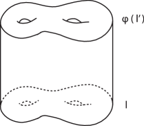
Figure 3: We consider Chern-Simon theory on $\Sigma\times I$, where the complex structure of the two Riemann surfaces on the boundary are specified by $l$ and $\varphi(l^{\prime})$.

3.4 $SL(2,\mathbb{R})$ Chern-Simons Reformulation of the Generalized AGT relation

In the discussion so far our aim has been to provide evidence for (2.11) and (2.15). However, we have already obtained more than we originally aimed for; all the ingredients of the generalized AGT relation (3.10) can now be expressed in the language of the Teichmüller theory, and consequently the $SL(2,\mathbb{R})$ Chern-Simons theory. This give a natural question: is there a natural interpretation of the whole expression (3.10), not just the 3d domain wall partition function?

Using the expression (3.20) for the conformal block in quantum Teichmüller theory, (3.13) becomes

$$\int dldl^{\prime}\,\nu(l)\nu(l^{\prime})\,\langle\bar{q}|l\rangle\langle l|\varphi|l^{\prime}\rangle\langle l^{\prime}|q\rangle.$$ (3.41)

Using the completeness relation of basis $|l\rangle$ (3.19), this reduces to a rather simple expression

$$\langle\bar{q}|\varphi|q\rangle=\langle\bar{q}|q^{\prime}\rangle.$$ (3.42)

Again, we have an expectation value of the operator $\varphi$, but now in the holomorphic basis. This is to be expected since conformal block represent the change of basis in quantum Teichmüller theory. (3.42) represents the two figures in Figure 2; for example, the right hand side simply says that we have a Janus solution with $\tau$ in the northern hemisphere and $\tau^{\prime}$ in the souther hemisphere, which is represented by a pairing between the states $|q\rangle$ and $|q^{\prime}\rangle$ in the Hilbert space $\mathcal{H}_{\rm CS}(\Sigma)$ (recall $q:=e^{2\pi i\tau}$).

The discussion so far raises the following question: is there a counterpart of the state $|q\rangle$ in 3d domain wall theory, not just its pairing? Is there a Hilbert space in 4d theory? Since the 4d theory near the domain wall is defined on $S^{3}\times I$, by regarding $I$ direction as time and canonically quantizing the theory we have a natural candidate, the Hilbert space of quantum ground states of the 4d theory on $S^{3}$. We are going to denote this by $\mathcal{H}_{\rm 4d}(S^{3})$. From this viewpoint the chiral half of the AGT relation can be formulated as an equivalence of two Hilbert spaces, $\mathcal{H}_{\rm 4d}(S^{3})$ and $\mathcal{H}_{L}(\Sigma)$, where as we have seen the latter coincides with $\mathcal{H}_{\rm CS}(\Sigma)$. Moreover, the Nekrasov partition function and the conformal block are represented by the same element in the Hilbert space in this identification:

$$\begin{split}\mathcal{H}_{\rm 4d}(S^{3})&=\mathcal{H}_{\rm L}(\Sigma),\\ \rotatebox{90.0}{$\in$}\hskip 14.22636pt&\hskip 14.22636pt\rotatebox{90.0}{$\in$}\\ |Z_{\rm Nek}\rangle&=|\mathcal{F}\rangle,\end{split}$$ (3.43)

and the equivalence of the 4d partition function (3.10) and (3.13) becomes a simple statement that an action of the matrix element of $\varphi$ commutes with the isomorphism between the Hilbert spaces of the two theories:

$$\langle\overline{Z_{\rm Nek}}|\varphi|Z_{\rm Nek}\rangle=\langle\overline{\mathcal{F}}|\varphi|\mathcal{F}\rangle.$$ (3.44)

The interpretation of the AGT correspondence as an identification of $\mathcal{H}_{\rm 4d}(S^{3})$ and $\mathcal{H}_{L}(\Sigma)$ is not new, see for example [17, 43]. The novelty of the present discussion is that we consider an action of the mapping class group and gave a Chern-Simons interpretation of the results.

There is actually one more Hilbert space in the literature. In [43], Nekrasov and Witten considered a 4d topologically twisted theory on $\Omega$-deformed 3-sphere, $S^{3}_{\epsilon_{1},\epsilon_{2}}$, where $\epsilon_{1},\epsilon_{2}$ are parameters of $\Omega$-deformation (3.2). Pestun’s result then means that quantum ground state of the physical string theory on $S^{3}\times\mathbb{R}$ coincides with the Hilbert space of the topological twisted theory on $\Omega$-deformed $S^{3}_{\epsilon_{1},\epsilon_{2}}$, with $\epsilon_{1}=\epsilon_{2}$. It is natural to extend this result to $b\neq 1$; quantum ground state of the physical string theory on $S^{3}_{b}$ should coincide with the Hilbert space of the topological twisted theory on $\Omega$-deformed $S^{3}_{\epsilon_{1},\epsilon_{2}}$:

$$\mathcal{H}_{\textrm{topological 4d}}(S^{3}_{\epsilon_{1},\epsilon_{2}})=\mathcal{H}_{\textrm{physical 4d}}(S^{3}_{b}).$$ (3.45)

It is an interesting problem to find out if this is correct. Note that both $S^{3}_{b}$ and $S^{3}_{\epsilon_{1},\epsilon_{2}}$ preserve the same symmetry $U(1)\times U(1)$. If (3.45) is correct, then by taking the limit $\epsilon\to 0$, our story should be directly related with the work of Nekrasov and Shatashvili [44]. Works are currently in progress in this direction.

As already explained, the simple structure of the left hand side in (3.44) has a geometric meaning: $\langle\bar{Z}|$ corresponds to a contribution from a northern hemisphere, $\varphi$ to a domain wall on $S^{3}$, and $|Z\rangle$ to a southern hemisphere. In other words, we have a decomposition of the 4-sphere

$$S^{4}=D^{4}\cup_{S^{3}}D^{4},$$ (3.46)

where $D^{4}$ is a disc (hemisphere) which has the equator $S^{3}$ as a boundary.

The counterpart of this decomposition in the $SL(2,\mathbb{R})$ Chern-Simons theory will be as follows. Choose a 3-manifold $M_{\tau}$ with boundary $\Sigma$ with complex structure $\tau$, such that the path integral of the Chern-Simons theory gives an element $|q\rangle\in\mathcal{H}(\Sigma)$. We then have a 3-manifold

$$M=M_{\tau}\cup_{\varphi}M^{\prime}_{\tau^{\prime}},$$ (3.47)

and

$$Z_{\rm 4d}(S^{4})=Z_{\rm CS}(M).$$ (3.48)

It is notable that the relation (3.48) claims an equivalence of the partition function of 4d $\mathcal{N}=2$ theory (with 3d 1/2 BPS defect) and 3d Chern-Simons theory!

Unfortunately, we have not been able to explicitly identify the manifold $M_{\tau}$ which gives rise to a state $|q\rangle$ in $\mathcal{H}(\Sigma)$. However, there is an interesting observation: the decomposition (3.47) is reminiscent of the Heegaard decomposition of 3-manifolds.

To describe this, let us define a genus $g$ handlebody $H_{g}$ as a 3-disc $D^{3}$ with $g$ handles attached to it (see Figure 4). The boundary of this 3-manifold is a genus $g$ Riemann surface without punctures, $\Sigma_{g}$. This means that when we have two handlebodies of the same genus $g$ and an element $\varphi$ of the mapping class group of $\Sigma_{g}$, we can glue two handlebodies to construct a closed 3-manifold.

$$M=H\cup_{\varphi}H^{\prime},$$ (3.49)

where $\varphi$ maps $\partial H$ to $\partial H^{\prime}$. This decomposition is called a Heegaard decomposition of $M$, $\Sigma$ is called a Heegaard surface, and $g$ the Heegaard genus. There is a theorem saying that every closed 3-manifold admits a Heegaard decomposition.

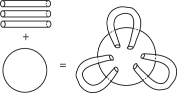
Figure 4: A genus $g$ handlebody is a 3-manifold obtained by attaching attaching $g$ handles to a 3-ball. Its boundary is a genus $g$ Riemann surface.

Comparing the two expressions (3.47) and (3.49), it is tempting to identify $M_{\tau}$ and $H$, when our Riemann surface $\Sigma=\Sigma_{g,h}$ does not have a puncture, $h=0$. This is a conjecture we make in this paper. If this turns out to be the case, $SL(2,\mathbb{R})$ partition function of an arbitrary 3-manifold, not just that on $\Sigma\times I$, has a direct interpretation in 4d $\mathcal{N}=2$ gauge theory. In fact, in the case of $SU(2)$ Chern-Simons theory, the same strategy was taken to define an invariant of the 3-manifold [45]. The method of the paper [45] applies directly to any rational conformal field theories, but not to irrational theories as discussed in this paper. It would be interesting to investigate this point in more detail.

Our proposed correspondence is summarized in Table 2.

Table 2: Summary of the proposed correspondence between 4d/3d gauge theory and $SL(2,\mathbb{R})$ Chern-Simons theory.

4d/3d gauge theory	3d $SL(2,\mathbb{R})$ Chern-Simons
$S^{4}$ with duality wall on $S^{3}$	3-manifold $M$
decomposition of $S^{4}$	Heegaard decomposition
$S^{4}$=$D^{4}\cup_{S^{3}}D^{4}$	$M=H_{1}\cup_{\Sigma}H_{2}$
disc $D^{4}$ with boundary $S^{3}$	handlebody $H$ with boundary $\Sigma$
duality wall $S^{3}$	mapping class group of $\Sigma$
quantum ground space of gauge theory	Hilbert space on the boundary
$\mathcal{H}_{\rm 4d}(S^{3}_{b})$	$\mathcal{H}_{\rm CS}(\Sigma)$
Nekrasov partition function $Z_{\rm Nek}\in\mathcal{H}_{\rm 4d}(S^{3}_{b})$	conformal block $\mathcal{F}\in\mathcal{H}_{\rm CS}(\Sigma)$
partition function on $S^{4}$	partition function on $M$

Comments on the M5-brane Interpretation

As already mentioned in introduction, the relation (2.11) can be considered as a 3+3 analog of the AGT relation, and has an M5-brane interpretation. Recall that AGT correspondence arises from M5-branes on $(S^{3}\times I)\times\Sigma$, where 4d $\mathcal{N}=2$ theory lives on $S^{3}\times I$ and 2d Liouville theory on $\Sigma$. In this language, our correspondence can be thought of as a M5-brane theory on $S^{3}\times(I\times\Sigma)$. In this sense our story can be considered as a (3+3) analog of AGT relation, where one theory (3d $\mathcal{N}=2$ domain wall theory) lives on $S^{3}$ and another ($SL(2,\mathbb{R})$ Chern-Simons theory) on $I\times\Sigma$. However, we should keep in mind the differences — our story includes extra domain walls, which breaks the supersymmetry to half ($\mathcal{N}=2$ in 3d), as opposed to 4d $\mathcal{N}=2$. In M-theory this will be represented by the existence of another M5-branes. The intersection of two M5-branes will be codimension 2 defects in the original M5-brane (cf. [2]). Brane configurations reminiscent of ours appears in the recent work of [46], which includes (as a particular case of more general brane setups) D3-branes wrapping $S^{4}$ and an NS5-brane on the equator $S^{3}$ inside $S^{4}$.

Before closing this section, let us comment on (possibly) related proposals in the literature. For example, [47, 48] conjectures a Chern-Simons description of 4d $\mathcal{N}=4$ theory on $S^{1}$ with twists by R-symmetry and S-duality. [6] proposes a correspondence between 3d $SL(2,\mathbb{C})$ Chern-Simons theory and 2d $\mathcal{N}=(2,2)$ theory, which could presumably be understood as a dimensional reduction of our story here. [50] discuss the Chern-Simons reformulation of AGT relation, and in particular makes contact with the results of [16, 17]. [51] also discusses the 3d hyperbolic geometry in the context of AGT relation and the work of [44], while the 2d Teichmüller/3d Chern-Simons connection as in section 4.4 has already appeared in [52]. The novelty of the present paper is that we have provided coherent presentation of all the topics from a unified perspective, starting from 4d/3d supersymmetric gauge theories to 3d $SL(2,\mathbb{R})$ Chern-Simons theory. We also have clarified the meaning of the AGT relation, and have provided exact quantitative statements (2.11), (2.15), which can be checked by explicit computations. It would be interesting to clarify the precise relation of our proposals and those in the literature. Some works in this direction is currently in progress [53].

4 Example: Once-Punctured Torus

In this section we work out the example of $\Sigma_{1,1}$ in detail. Many of the our results below can straightforwardly be adopted for more general examples (although computationally more complicated), and we have included several arguments which are independent of the example we discuss here.

4.1 Theories on Duality Walls

Let us begin with the description of the mother 4d $\mathcal{N}=2$ theory and its daughter, the 3d $\mathcal{N}=2$ domain wall theory. For once-punctured torus, the mother 4d theory is the 4d $\mathcal{N}=2^{*}$ theory, where the parameter associated with the puncture of $\Sigma_{1,1}$ plays the role of an adjoint mass parameter deforming $\mathcal{N}=4$ to $\mathcal{N}=2^{*}$. The mapping class group of $\Sigma_{1,1}$ is given by $SL(2,\mathbb{Z})$, which is identified with the S-duality group of the mother 4d theory.

What we would like to do is to identify the action of this group on the 3d $\mathcal{N}=4$ theory. This $SL(2,\mathbb{Z})$ action is not a symmetry of the 3d theory itself; rather it maps one 3d theory to a different 3d theory. This $SL(2,\mathbb{Z})$ action was studied by [55] for an Abelian gauge group, and by [4] for non-Abelian gauge groups.

Let us choose generators $S,T$ of $SL(2,\mathbb{Z})$:

$$S=\left(\begin{array}[]{cc}0&1\\ -1&0\end{array}\right),\quad T=\left(\begin{array}[]{cc}1&1\\ 0&1\end{array}\right).$$ (4.5)

An arbitrary element $\varphi$ of $SL(2,\mathbb{Z})$ can then be written as

$$\varphi=T^{n_{1}}ST^{n_{2}}ST^{n_{3}}\ldots ST^{n_{k}}.$$ (4.6)

It is therefore sufficient to identify the action of $T$ and $S$.

It is not difficult to describe the effect of $T$ transformations. $T^{k}$ maps $\tau$ to $\tau+k$, which means the shift of the $\theta$-angle by $2\pi k$. When we have a Janus configuration with $\theta$-angle profile given by

$$\theta(x_{3})=\begin{cases}2\pi k&(x_{3}>0),\\ 0&(x_{3}<0),\end{cases}$$ (4.7)

this induces a level $k$ Chern-Simons term on the 3d domain wall at $x_{3}=0$:

$$\frac{1}{8\pi^{2}}\int_{\mathbb{R}^{3}\times\mathbb{R}}\!\theta(x_{3})\,\textrm{Tr}\,F\wedge F=\frac{k}{4\pi}\int_{\mathbb{R}^{3}}\textrm{Tr}\,A\wedge\left(dA+\frac{2}{3}A^{3}\right),$$ (4.8)

Hence $T^{k}$ corresponds to adding a level $k$ Chern-Simons term for the background gauge field.

The effect of $S$-operation is more subtle. For the moment let us set the parameter $m$ to be zero, i.e., the 4d theory is the $\mathcal{N}=4$ theory, and discuss the mass deformation later.

To describe S-operation, let us introduce a 3d theory $T[SU(2)]$. This is a theory on the duality domain wall for $\varphi=S$. This is a 3d $\mathcal{N}=4$ SQED with two electron hypermultiplets. This theory has been extensively studied in the context of 3d mirror symmetry [56], and is self-mirror.

In $\mathcal{N}=2$ language, we have a vector multiplet $A$, an adjoint (i.e. neutral) hypermultiplet $\Phi$, and a set of hypermultiplets $\phi_{1},\phi_{2},\tilde{\phi}_{1},\tilde{\phi}_{2}$ of charge $+1,+1,-1,-1$. The theory has R-symmetry $\textrm{Spin}(4)=SU(2)_{N}\times SU(2)_{R}$, and a pair of hypermultiplets $(\phi_{i},\tilde{\phi_{i}})$ is a doublet of $SU(2)_{N}$. The theory has a Lagrangian

$$\begin{split}\mathcal{L}=\int\!d^{4}\theta\left[\frac{1}{g^{2}}\left(-\frac{1}{4}\Sigma^{2}+\Phi^{\dagger}\Phi\right)+\left(\phi_{i}{}^{\dagger}e^{-2V}\phi_{i}+\tilde{\phi}_{i}{}^{\dagger}e^{2V}\tilde{\phi}_{i}\right)\right]+\int\!d^{2}\theta\left[\sqrt{2}\tilde{\phi_{i}}\Phi\phi_{i}+\textrm{c.c.}\right],\end{split}$$ (4.9)

where $\Sigma$ is a linear multiplet containing the field strength of the vector multiplet. This theory has global symmetry $SU(2)\times SU(2)^{\vee}$, where $SU(2)^{\vee}=SO(3)$ is the Langlands dual of $SU(2)$. The $SU(2)$ symmetry manifest in the action, and $\phi_{i}$ ($\tilde{\phi_{i}}$) transform as a fundamental (antifundamental) of that $SU(2)$. The $SU(2)^{\vee}$ symmetry is not present in the classical action, and arises as a quantum symmetry of the theory (the Abelian part of $SU(2)^{\vee}$ is simply a shift of the dual photon, but we need to use monopole operators to see other symmetries).

We can introduce a real mass parameter $\mu$ and a FI parameter $\zeta$. The former is introduced by gauging the $U(1)$ part of the flavor symmetry $SU(2)$ and introducing a background gauge field $V_{\mu}=-i\theta\bar{\theta}\mu$. Since the four hypermultiplets $\phi_{1},\phi_{2},\tilde{\phi}_{1},\tilde{\phi}_{2}$ have charges $+1,-1,-1,+1$, this adds a term

$$\mathcal{L}_{\mu}=\int\!d^{4}\theta\left[\phi_{1}^{\dagger}e^{-2V_{\mu}}\phi_{1}+\phi_{2}^{\dagger}e^{2V_{\mu}}\phi_{2}+\tilde{\phi}_{1}^{\dagger}e^{2V_{\mu}}\tilde{\phi}_{1}+\tilde{\phi}_{2}^{\dagger}e^{-2V_{\mu}}\tilde{\phi}_{2}\right].$$ (4.10)

to the Lagrangian. The FI parameter is similarly introduced by coupling a background vector multiplet

$$\mathcal{L}_{\zeta}=-\frac{4}{\pi}\int\!d^{4}\theta\,V_{\zeta}\Sigma,$$ (4.11)

where $V_{\zeta}=i\theta\bar{\theta}\zeta$ and the numerical factor in front of the integral is chosen for later convenience.

Now let us go back to the action of $S$ on 3d $\mathcal{N}=4$ gauge theories. Let us begin with a 3d superconformal theory with a $SU(2)$ global symmetry. Since $T[SU(2)]$ has global symmetry $SU(2)\times SU(2)^{\vee}$, we can gauge the diagonal part of the two $SU(2)$ global symmetries of the two theories. The resulting theory has a global symmetry $SU(2)^{\vee}$, which is a remnant of the global symmetry of $T[SU(2)]$. Similarly, when we have a theory with global symmetry $SU(2)^{\vee}$, we can couple it to $T[SU(2)^{\vee}]$ (which is $T[SU(2)]$ due to mirror symmetry) and the resulting theory has a global symmetry $SU(2)$. This is the action of $S$ on 3d theories.

$S$ and $T$ defined above satisfy [55, 4]

$$S^{2}=1,\quad(ST)^{3}=1,$$ (4.12)

and hence generate the full $SL(2,\mathbb{Z})$.

It is useful to graphically represent $S$ and $T$ as in Figure 5. In this figure, gauging the diagonal $G$ symmetry ($G=SU(2)$ or $SU(2)^{\vee}$) of two theories with $G$ global symmetry is represented by concatenating two edges. Our 3d theory corresponding to an element of the mapping class groups is described by a linear quiver, while the 3d theory in (2.15) is described by a circular quiver.

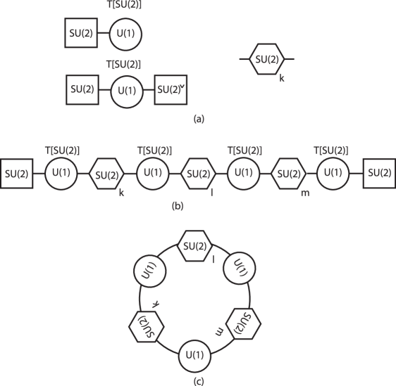
Figure 5: Graphical representation of $S$ and $T$ operations on 3d $\mathcal{N}=4$ theory. In these figures a square represents a global symmetry, a circle gauge symmetry, and a hexagon a Chern-Simons term, with level specified by an integer written nearby. In (a) we listed all the basic building block of our quiver. The left represents our $T[SU(2)]$ theory. This is often written as above, with only $SU(2)$ symmetry manifest. However, it also has quantum $SU(2)^{\vee}$ symmetry, and in the figure below we have also shown this symmetry explicitly. The figure on the right represents the action of T, i.e., Chern-Simons couplings. More generally, an element of the mapping class group is represented by a product of $S$ and $T$, and graphically represented by a linear quiver. The example of $\varphi=ST^{k}ST^{l}ST^{m}S$ is given in (b). When we gauge the remaining $SU(2)\times SU(2)$ symmetry, we have a circular quiver, given in (c). In figures (b) and (c) we neglected subtle differences between $SU(2)$ and $SU(2)^{\vee}$.

Let us now give mass to the adjoint hypermultiplet, and deform $\mathcal{N}=4$ theory to $\mathcal{N}=2^{*}$ theory. The corresponding deformation in 3d daughter theory was identified in [18] based on symmetry arguments: the deformation should preserve $SU(2)\times SU(2)^{\vee}$ symmetry as well as $\mathcal{N}=2$ supersymmetry. The answer is that we weakly gauge the $U(1)$ symmetry under which $\phi_{i},\tilde{\phi}_{i}$ all have charge $1$ and $\Phi$ charge $-2$. The action now contains an extra term

$$\mathcal{L}_{m}=\int\!d^{4}\theta\left[\Phi^{\dagger}e^{4V_{m}}\Phi+\sum_{i=1}^{2}\left(\phi_{i}^{\dagger}e^{-2V_{m}}\phi_{i}+\tilde{\phi}_{i}^{\dagger}e^{-2V_{m}}\tilde{\phi}_{i}\right)\right],$$ (4.13)

where $V_{m}=im\theta\bar{\theta}/2$. The factor 2 is chosen for notational simplicity of the following discussion.

Partition Function on Deformed $S^{3}$

We are now going to compute the partition function on $S^{3}$, or more generally the deformed 3-sphere $S^{3}_{b}$. We can use localization [57], as well as its generalization to theories with anomalous dimensions [58, 59], to compute the partition function on $S^{3}$. More recently, these computations has been generalized to the deformed $S^{3}_{b}$ [60].

The partition function for the mass-deformed $T[SU(2)]$, given in [18, 59] for $b=1$ and here generalized to $b\neq 1$, reads

$$Z_{T[SU(2);m]}(\mu,\zeta;m)=\frac{1}{s_{b}(m)}\int\!d\sigma\,\frac{s_{b}(\mu+\sigma+\frac{m}{2}+\frac{iQ}{4})s_{b}(\mu-\sigma+\frac{m}{2}+\frac{iQ}{4})}{s_{b}(\mu+\sigma-\frac{m}{2}-\frac{iQ}{4})s_{b}(\mu-\sigma-\frac{m}{2}-\frac{iQ}{4})}\,e^{4\pi i\zeta\sigma}.$$ (4.14)

In this expression the four dilogarithms arise from the 1-loop determinants of four hypermultiplets. The integration variable $\sigma$ is a scalar of the vector multiplet, and the exponential term in the integrand represents the classical contribution from the vector multiplet. 1-loop determinant is trivial for the vector multiplet. Finally, the factor $1/s_{b}(m)$ arises from the 1-loop determinant for the neutral hypermultiplet. Mirror symmetry can be formulated as a statement

$$Z_{T[SU(2);m]}(\mu,\zeta;m)=Z_{T[SU(2);m]}(\zeta,\mu;-m).$$ (4.15)

We can also generalize this analysis to a linear quiver, i.e. more general element of $SL(2,\mathbb{Z})$ as in Figure 5 (b). When we gauge $SU(2)$ global symmetry ($SU(2)^{\vee}$ symmetry), the background vector fields represented by the mass parameter $\mu$ (FI parameter $\zeta$) becomes dynamical, and should be regarded as a scalar component $\sigma$ of the vector multiplet. In localization, this is the variable over which we integral out. This means that when we take a product of two elements in $SL(2,\mathbb{Z})$, we need to take a product of the partition function of the corresponding two theories and integrate over the scalar component of the vector multiplet which becomes dynamical. For example, for $\varphi=ST^{k}S$ we have

$$\int\!d\sigma\,Z_{T[SU(2);m]}(\mu,\sigma)\,e^{-4\pi ik\sigma^{2}}\,Z_{T[SU(2);m]}(\sigma,\mu^{\prime}),$$ (4.16)

where the term $e^{-4\pi ik\sigma^{2}}$ represents the classical contribution from the Chern-Simons term induced by the action of $T^{k}$. When we introduce integral kernels

$$S_{(\sigma,\sigma^{\prime};m)}:=Z_{T[SU(2);m]}(\sigma,\sigma^{\prime};m),\quad T_{(\sigma,\sigma^{\prime})}:=e^{-4\pi i\sigma^{2}}\delta(\sigma-\sigma^{\prime}),$$ (4.17)

the expression (4.16) then simplifies to

$$\int\!d\sigma d\sigma^{\prime}\,S_{(\mu,\sigma;m)}T^{k}_{(\sigma,\sigma^{\prime})}S_{(\sigma^{\prime},\mu^{\prime};m)}=(ST^{k}S)_{(\mu,\mu^{\prime};m)}.$$ (4.18)

Namely, $\varphi$ is simply a product of matrices given in (4.17)! It is therefore straightforward to compute the partition function for the theory $T[SU(2);\varphi;m]$ for any element of $\varphi$ of $SL(2,\mathbb{Z})$.

This statement, despite its simplicity, is actually far from trivial. The potential source of trouble is that (as mentioned already) the classical Lagrangian of $T[SU(2);m]$ has only $SU(2)$ symmetry, and $SU(2)^{\vee}$ is a quantum symmetry which is not present in the Lagrangian. We can switch to the mirror description to make $SU(2)^{\vee}$ symmetry manifest, but then $SU(2)$ symmetry is turned into a quantum symmetry. What this means is that at the Lagrangian level it is not clear how to gauge both $SU(2)$ symmetry and $SU(2)^{\vee}$ symmetry simultaneously, but such a simultaneous gauging of $SU(2)$ and $SU(2)^{\vee}$ is needed for constructing theories with longer quivers including three or more $S$, say $\varphi=ST^{k}ST^{l}S$ . In this paper, motivated by the correspondence with Liouville theory and Chern-Simons theory, we conjecture that the partition function in these cases can still be computed from the products of (4.17). Alternatively, we can regard our Gauge/Liouville/Teichmüller/Chern-Simons correspondence as a supporting evidence for this conjecture. It would be interesting to explicitly verify this conjecture.

4.2 Comparison with Liouville Theory

Let us next compare out results in 3d gauge theory with the modular transformation properties of conformal blocks in Liouville theory (3.12). Again, an element $\varphi$ of $SL(2,\mathbb{Z})$ can be decomposed into a product of $S$’s and $T$’s, and all we need to do is to write down the integral kernel for $S$ and $T$. For the $T$ transformation, we have

$$T_{(\alpha,\alpha^{\prime};E)}=\delta(\alpha-\alpha^{\prime})e^{4\pi i\Delta(\alpha)},$$ (4.19)

where $\Delta(\alpha)$ is the conformal dimension given in (3.4). For the S-kernel the expression in [62, 22] reads

$$S_{(\alpha,\alpha^{\prime},E)}=\frac{2^{3/2}}{s_{b}(E)}\int_{\mathbb{R}}dr\frac{s_{b}(\alpha^{\prime}+r+\frac{E}{2}+\frac{iQ}{4})s_{b}(\alpha^{\prime}-r+\frac{E}{2}+\frac{iQ}{4})}{s_{b}(\alpha^{\prime}+r-\frac{E}{2}-\frac{iQ}{4})s_{b}(\alpha^{\prime}-r-\frac{E}{2}-\frac{iQ}{4})}e^{4\pi\alpha r},$$ (4.20)

where the function $s_{b}(x)$ is the quantum dilogarithm function [63, 64, 8] defined in the appendix B.

By comparing the formulas (4.14), (4.17) and (4.19), (4.20), we see that the two result much under the parameter identification

$$r=\sigma,\quad\alpha=\zeta,\quad\alpha^{\prime}=\mu,\quad E=m.$$ (4.21)

This explicitly verifies the relation (3.14).

4.3 Construction of the Hilbert Space

Having established the connection between 3d $\mathcal{N}=2$ theory and Liouville theory, we move on to quantum Teichmüller theory. Readers unfamiliar with Teichmüller theory are encouraged to consult appendix A.

Figure 6: Triangulation of $\Sigma_{1,1}$. The fundamental region of the torus is represented by a square, and the puncture are represented by four black dots, all of which are identified. The triangulation has two triangles and three edges.

Let us triangulate our surface $\Sigma_{1,1}$ by 3 edges and 2 triangles, as shown in Figure (6). For each of the 3 edges we assign a Fock coordinate, denoted by $x,y$ and $z$. The non-trivial commutation relations are given by (A.10)

$$[\mathsf{x},\mathsf{y}]=[\mathsf{y},\mathsf{z}]=[\mathsf{z},\mathsf{x}]=-4\pi ib^{2},$$ (4.22)

or equivalently

$$\mathsf{X}\mathsf{Y}=q^{-4}\mathsf{Y}\mathsf{X},\quad\mathsf{Y}\mathsf{Z}=q^{-4}\mathsf{Z}\mathsf{Y},\quad\mathsf{Z}\mathsf{X}=q^{-4}\mathsf{X}\mathsf{Z},$$ (4.23)

where in the following capitalized variables represent exponentiation,

$$\mathsf{X}=e^{\mathsf{x}},\quad\mathsf{Y}=e^{\mathsf{y}},\quad\mathsf{Z}=e^{\mathsf{z}}.$$ (4.24)

This algebra has a central element, i.e. a constant, corresponding to the puncture

$$m:=\mathsf{x}+\mathsf{y}+\mathsf{z}.$$ (4.25)

There are 2 remaining variables, which is consistent with the fact that the complex dimension of the Teichmüller space is one in this example (see (2.5)). Let us choose the 2 variables to be $\mathsf{r}$ and $\mathsf{s}$, which are defined by

$$2\pi b\,\mathsf{r}=\frac{\mathsf{y}+\mathsf{z}}{2},\quad 2\pi b\,\mathsf{s}=\frac{\mathsf{y}-\mathsf{z}}{2}.$$ (4.26)

Note that this particular choice of variables breaks the $SL(2,\mathbb{Z})$ symmetry of the torus. They satisfy the standard commutation relation

$$[\mathsf{s},\mathsf{r}]=\frac{1}{2\pi i}.$$ (4.27)

This commutation relation has a standard representation in terms of coherent state of $q$:

$$\mathsf{r}|r\rangle=r|r\rangle,\quad\mathsf{s}|r\rangle=\frac{1}{2\pi i}\frac{\partial}{\partial r}|r\rangle.$$ (4.28)

This is an infinite dimensional representation, reflecting the fact the Liouville theory is an irrational conformal field theory.

Let us next describe the action of the mapping class group $SL(2,\mathbb{Z})$. For this purpose it is useful to choose the generators

$$L=\left(\begin{array}[]{cc}1&1\\ 0&1\end{array}\right),\quad R=\left(\begin{array}[]{cc}1&0\\ 1&1\end{array}\right).$$ (4.33)

More concretely, these flips change the $\alpha,\beta$-cycles of the torus as

$$L:\alpha\to\alpha+\beta,\beta\to\beta,\quad R:\alpha\to\alpha,\beta\to\alpha+\beta.$$ (4.34)

These generators are related to the generators $S$ and $T$ (4.5) by

$$S=LR^{-1}L,\quad T=L.$$ (4.35)

The action of $L$ can be considered as a product of the flip on the edge $x$, together with the exchange of labels of $x$ and $z$ afterwards, see Figure (7). The flip is represented by (A.13)

$$\mathsf{X}^{\prime}=\mathsf{X}^{-1},\quad\mathsf{Y}^{\prime}=(1+q\mathsf{X})(1+q^{3}\mathsf{X})\mathsf{Y},\quad\mathsf{Z}^{\prime}=(1+q\mathsf{X}^{-1})^{-1}(1+q^{3}\mathsf{X}^{-1})^{-1}\mathsf{Z}.$$ (4.36)

The variables $\mathsf{X}^{\prime},\mathsf{Y}^{\prime},\mathsf{Z}^{\prime}$ satisfy

$$\mathsf{X}^{\prime}\mathsf{Y}^{\prime}=q^{4}\mathsf{Y}^{\prime}\mathsf{X}^{\prime},\quad\mathsf{Y}^{\prime}\mathsf{Z}^{\prime}=q^{4}\mathsf{Z}^{\prime}\mathsf{Y}^{\prime},\quad\mathsf{Z}^{\prime}\mathsf{X}^{\prime}=q^{4}\mathsf{X}^{\prime}\mathsf{Z}^{\prime}.\quad$$ (4.37)

We need to exchange $\mathsf{X}$ and $\mathsf{Z}$ in order to go back to the original algebra (4.23). We then have an expression for the action of $L$:

$$\mathsf{X}^{\prime\prime}=(1+q\mathsf{X}^{-1})^{-1}(1+q^{3}\mathsf{X}^{-1})^{-1}\mathsf{Z},\quad\mathsf{Y}^{\prime\prime}=(1+q\mathsf{X})(1+q^{3}\mathsf{X})\mathsf{Y},\quad\mathsf{Z}^{\prime\prime}=\mathsf{X}^{-1}.$$ (4.38)

The operator $\mathsf{L}$ for an element $L$ of the mapping class group reproduces this

$$\mathsf{X}^{\prime\prime}=\mathsf{L}^{-1}\,\mathsf{X}\,\mathsf{L}~{}~{},\quad\mathsf{Y}^{\prime\prime}=\mathsf{L}^{-1}\,\mathsf{Y}\,\mathsf{L}~{}~{},\quad\mathsf{Z}^{\prime\prime}=\mathsf{L}^{-1}\,\mathsf{Z}\,\mathsf{L}~{}~{},\quad$$ (4.39)

and we have a similar set of equations for $\mathsf{R}$.

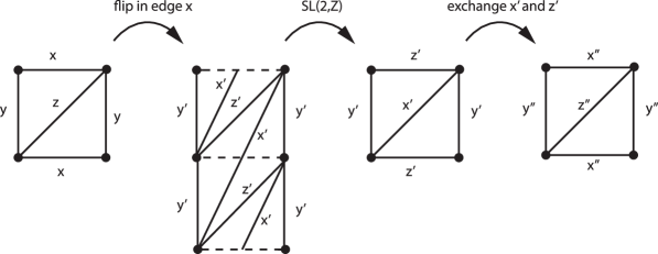
Figure 7: $L$ acts on the triangulation by a combination of a flip with an exchange of labels of edges.

4.4 Chern-Simons Reformulation

Armed with the construction of the Hilbert space in the previous section, we can now give a precise prescription to define the Chern-Simons partition functions in (2.11), (2.15). Here we concentrate on the trace $\textrm{Tr}\,\varphi$, but the same argument can straightforwardly be adopted for $\langle l|\varphi|l^{\prime}\rangle$.

Again, let us fix a triangulation of $\Sigma$. The element $\varphi$ of the mapping class group maps this triangulation to another. Since any two triangulations are related by flips, the action of $\varphi$ on the Hilbert space can be represented by a product of operators representing flips.

$$\varphi=\mathsf{T}_{1}\mathsf{T}_{2}\ldots\mathsf{T}_{N},$$ (4.40)

where in the example here, $\mathsf{T}_{i}$ is either one of the two operators $\mathsf{L}$ or $\mathsf{R}$. The decomposition of $\varphi$ into flips is not unique, but the expression (4.40) is well-defined due to the pentagon relation. By inserting a complete set of basis

$$\int\!dq_{i}\,|q_{i}\rangle\langle q_{i}|=1.$$ (4.41)

we have

$$\textrm{Tr}(\varphi)=\int\prod_{i}dq_{i}\,\langle q_{1}|\mathsf{T}_{1}|q_{2}\rangle\langle q_{2}|\mathsf{T}_{2}|q_{3}\rangle\ldots\langle q_{N}|\mathsf{T}_{N}|q_{1}\rangle.$$ (4.42)

As for the basis $|q_{i}\rangle$, we can either take $|x\rangle$ or its conjugate $|y\rangle$. Note that the expression above is independent of the choice of basis $|q_{i}\rangle$, since we are computing the trace.

This discussion so far can be summarized in the following rules:

1. Decompose the action of $\varphi$ into a product of flips.

2. For each flip we prepare a “wave function” $\langle q|\mathsf{T}|q^{\prime}\rangle$. Here $q$ and $q^{\prime}$ are different only in quadrilateral where the flip $\mathsf{T}$ takes place. In other words, this is a local operation on $\Sigma$.

3. We glue the wave functions, where gluing means we integrate over the variables shared by two flips. For example, the gluing of two wavefunction $\langle q|\mathsf{T}|q^{\prime}\rangle$ and $\langle q^{\prime}|\mathsf{T}^{\prime}|q^{\prime\prime}\rangle$ is performed as

   $$\int\!dq^{\prime}\,\langle q|\mathsf{T}|q^{\prime}\rangle\langle q^{\prime}|\mathsf{T}^{\prime}|q^{\prime\prime}\rangle,$$ (4.43)

   and this gives another wavefunction $\langle q|\mathsf{T}\mathsf{T}^{\prime}|q^{\prime\prime}\rangle$. By repeating this procedure, the trace $\textrm{Tr}(\varphi)$ is obtained by integrating over all the intermediate states $|q\rangle$.

Note that the trace is independent of the choice of triangulation we started with. Indeed, when we change the triangulation we change the initial state $|q_{1}\rangle$ to $|q_{1}^{\prime}\rangle=\mathsf{T}|q_{1}\rangle$, where $\mathsf{T}$ represents a product of flips. This has the effect of replacing $\varphi$ by $\mathsf{T}^{-1}\varphi\mathsf{T}$, but this does not change the trace since the trace is invariant under conjugation.

Now let us reformulate these rules in terms of the 3d $SL(2,\mathbb{R})$ Chern-Simons theory. Recall that our 3-manifold relevant for the computation of $\textrm{Tr}\,\varphi$ is a mapping torus (2.14). In most of the cases the 3-manifold is a hyperbolic manifold, locally isomorphic to $\mathbb{H}^{3}$. For example, for $\varphi=LR$ we have a complement of the figure eight knot (also called $4_{1}$ knot, see Figure 8), $\varphi=L^{2}R$ is a hyperbolic manifold called m009 in the conventions of SnapPea.

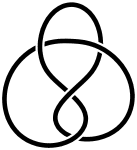
Figure 8: The figure eight knot. This is a knot inside $S^{3}$, and the complement of this knot is a mapping torus of $\Sigma_{1,1}$ over $S^{1}$, with $\varphi=LR$.

The key observation for the following discussion is that a flip can be traded for a tetrahedron [65], see Figure 9. Suppose that we have a flip in a quadrilateral. We can then introduce an extra direction (time coordinate) to represent this change as a cube, see Figure 9 (b). By taking a deformation retract of this cube, we have a tetrahedron of the pillow-like shape (Figure 9 (c)). This tetrahedron is essentially the superposition of the two quadrilaterals in Figure 9 (a).

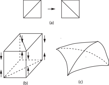
Figure 9: A flip in 2d can be traded for a tetrahedron in 3d. The tetrahedron (c) is obtained by a deformation retract of the cube (b) representing the flip (a).

This means that the decomposition of $\varphi$ into flips in 2d now becomes a decomposition of the 3-manifold into tetrahedra in 3d language. The gluing operation in the third step of the previous rule then becomes the gluing two faces of the tetrahedra.

In our example of once-punctured torus, when $\varphi$ is written as product of $N$ generators $L$ and $R$, the mapping torus is triangulated with $N$ tetrahedra. We can take these tetrahedra to be ideal tetrahedra, where an ideal tetrahedron is a tetrahedron with vertices at the boundaries of $\mathbb{H}^{3}$ in a hyperbolic manifold [65].

Our new rule, now in 3d language, is summarized as follows.

1. Decompose the mapping torus into tetrahedra

   $$M=\bigcup_{i}\Delta_{i},$$ (4.44)

2. For each tetrahedron we prepare a matrix element $\langle q|\mathsf{T}|q^{\prime}\rangle$. $|q\rangle$ and $|q^{\prime}\rangle$ now represent the boundary conditions at the faces of the tetrahedron.

3. When we glue two ideal tetrahedra, we glue the two corresponding wave functions by integrating over boundary conditions. The partition function on $M$ is obtained by gluing all the ideal tetrahedra as in (4.44).

Some readers might think at this moment that this is just a trivial rewriting of what we already know. However, all of the above 3 steps are given intrinsically in 3d, and in particular, we can choose triangulations different from the ones coming from the triangulation of the 2d surface $\Sigma$. Any two 3d ideal triangulations are related by a series of 2-3 Pachner moves shown in Figure 10, and pentagon relation in 2d can now be interpreted as an invariance of our partition function under the 2-3 Pachner move.

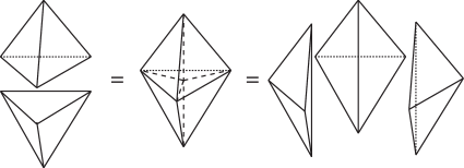
Figure 10: The 2-3 Pachner move. This move changes a 3d ideal triangulation into another.

The partition function defined by the procedure above is a kind of a state sum model for the Chern-Simons theory. The basic idea is the same as our previous discussion of Chern-Simons theory as TQFT, except that we now apply the same procedure to each tetrahedra. Namely, we have a wave function (an element in the Hilbert space) for each tetrahedron when we do the path integral over the tetrahedron with specific boundary conditions. There are some well-known state sum models for Chern-Simons theory, see [67, 68]. For the case of direct relevance to our paper, i.e. $SL(2,\mathbb{R})$ Chern-Simons theory or its analytic continuation into $SL(2,\mathbb{C})$, there is a proposed state sum model by Hikami [69, 66], which is a non-compact analog of [70]. See also [71, 72, 73]. It is an interesting problem to compare the our state sum model with the known results in the literature. This problem is currently under investigation [53].

Finally, let us conclude this section by briefly commenting on more general Riemann surfaces. The procedure is in principle the same for any Riemann surface, but can be technically involved. Probably the next simplest example will be a 4-punctured sphere, which corresponds to 4d $SU(2)$ $N_{f}=4$ theory. The integral kernel of the fusion and branding for this theory are known (see for example [75]). Indeed, the S-transformation for $\Sigma_{1,1}$ is a specialization of that of $\Sigma_{0,4}$ [76]. Both $\Sigma_{1,1}$ and $\Sigma_{0,4}$ are covered by $\Sigma_{1,4}$.

5 Comments on Higher Rank Generalizations

It is straightforward to generalize our proposal to the case $G=SU(N)$. This claims the equivalence of the partition function of 3d $SL(N,\mathbb{R})$ Chern-Simons theory on a 3-manifold $\Sigma\times I$ with that of a 3d $\mathcal{N}=2$ $SU(N)$ gauge theory on a (deformed) 3-sphere $S^{3}$ ($S^{3}_{b}$), which is realized as a duality domain wall inside the mother 4d $\mathcal{N}=2$ $SU(N)$ theory on $S^{4}$.

Many of the ideas presented in section 3 have their counterparts in this higher rank generalization. For example, AGT relation has been generalized to $SU(N)$ gauge groups by [77, 78]. Moreover, there exists are higher rank generalization of Teichmüller theory called the higher Teichmüller theory [79], which quantizes the moduli space of flat $SL(N,\mathbb{C})$ or $SL(N,\mathbb{R})$ connections for $N>2$ [80]. As for the boundary conditions of Chern-Simons theory, there is again a Hamiltonian reduction from $SL(N,\mathbb{C})$ Chern-Simons theory to Toda theory on the boundary [37, 38, 39]. Moreover, the computation of partition functions by localization works for $SU(N)$ gauge theories both for 3d and 4d theories. It would be interesting to perform detailed quantitative checks of this generalization.

6 Conclusion and Discussion

In this paper, we initiated a program to connect 3d $SL(2,\mathbb{R})$ Chern-Simons theory and 3d $\mathcal{N}=2$ gauge theory on duality walls. In particular, we proposed an equality of the partition functions of the two theories, given in (2.11) and (2.15). We also proposed a $SL(2,\mathbb{R})$ reformulation of the AGT relation and its generalization (see Table 2). We provided evidence for this conjecture by linking the two theories with quantum Liouville theory and quantum Teichmüller theory. We also provided explicit computations in the case of the once-punctured torus.

Clearly there are many open problems, some of which are already mentioned in the main text. Here we list some more problems. Solutions to any of these questions are welcome.

• Identify the matter content of the 3d $\mathcal{N}=2$ domain wall theory for general Riemann surface $\Sigma_{g,h}$. This should be a doable problem since the partition function of these theories can be computed from quantum Teichmüller theory.

• Can we give a direct verification of our proposal from dimensional reduction of 6d $(2,0)$ theory? As a possible clue, [82] discuss the appearance of the Chern-Simons term from a dimensional reduction of $(2,0)$ theory.

• Does our 4d partition function give an invariant of a 3-manifold determined from a Heegaard decomposition (see section 3.4)? Alternatively, one may use the definition from the surgery formula, mimicking the argument of [35].

• Identify the quantum group $U_{q}(SL(2,\mathbb{R}))$ in our story, see for example [75]. For $SU(2)$ Chern-Simons theory the quantum group $U_{q}(SU(2))$ was used in the mathematical formulation of the 3-manifold invariants [83].

• $SL(2,\mathbb{C})$/$SL(2,\mathbb{R})\times SL(2,\mathbb{R})$ Chern-Simons theory describe the Lagrangian of 3d gravity [84]. Is there any implication of our results to 3d gravity? Since Liouville theory describes 2d gravity, there should be a relation between 3d gravity and 2d gravity, which in turn is related to 4d/3d supersymmetry gauge theory.

• Extend our results to asymptotically free 4d gauge theories [85, 86] or 5d gauge theories [87, 88].

• Study the self-duality of $SL(2,\mathbb{R})$ Chern-Simons theory, see discussion around (2.17) and [73] for recent discussion. Mathematically, this is a manifestation of the (quantum ) geometric Langlands correspondence, see for example [89, 90, 91, 92, 93, 26].

• Formulas of quantum dilogs appear in the Kontsevich-Soibelman wall crossing formula [94]. Is there any implication of our results to wall crossing? The reference [95] uses Fock coordinates to give physical derivation of the wall crossing formula, and the trace similar to ours appear in [96].

• Prove (3.45). Connect our story to that of [44, 43, 26, 97], and find integrable structures in Chern-Simons theory.

• Find a gravity solution representing our M5-brane configurations in the large $N$ limit. The gravity solution constructed in [98] may be useful in this respect.

• Reformulate/prove our conjectures in the language of Penner-type matrix models, see [99].

• The dual graph of the triangulation of $\Sigma$ is a bipartite graph (dimer), which also appears in the context of 4d quiver gauge theories [100, 101, 102] and BPS state counting on toric Calabi-Yau manifolds [103, 104, 105]. There are similarities between quantum Teichmüller theory and dimer theory, cf. [106]. How far does this analogy go?

Appendix A Construction of the Teichmüller Hilbert Space

In this section we summarize basic aspects of the classical and quantum Teichmüller theory. This gives a precise recipe to construct the Hilbert space $\mathcal{H}_{T}(\Sigma)$. Our discussion here applies to a general Riemann surface $\Sigma_{g,h}$. See section 4 for a concrete discussion in the case of $\Sigma_{1,1}$.

A.1 Fock coordinates and Flips

Let us begin by introducing coordinates in the Teichmüller space. The basic idea needed for this is simple — by triangulating a Riemann surface, we can divide $\Sigma$ into a set of triangles, and by explicitly specify how we glue these triangles back we can parametrize the complex structure moduli of $\Sigma$.

The triangulation is chosen in such a way that all the vertices of the triangles are placed at the punctures and all edges are geodesics connecting punctures. Here geodesic means geodesic in the metric corresponding to a point in the Teichmüller space. The number of faces ($F$), edges ($E$) and vertices ($V$) are given by

$$F=2(2g-2+h),\quad E=3(2g-2+h),\quad V=h.$$ (A.1)

To verify this, note the constraints

$$3F=2E,\quad\chi(\Sigma_{g,0})=-V+E-F=2g-2.$$ (A.2)

It is known that all such triangulation are related by a series of operations called flips (also called Whitehead moves). Choose an edge $e$ which bounds two triangles. A flip removes the edge $e$ and adds another diagonal $e^{\prime}$ of the resulting quadrilateral (see Figure 11). Flips satisfy the pentagon relation shown in Figure 11, which can be represented by

$$T_{12}T_{13}T_{23}=T_{23}T_{12},$$ (A.3)

where $T_{ij}$ represents the flip exchanging the two neighboring faces $i$ and $j$.

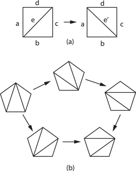
Figure 11: (a) represents a flip on the edge $e$. (b) shows the pentagon relation.

Given a triangulation, we assign a coordinate $z_{e}$, the Fock coordinate (also called the shear coordinate) [107], for each edge $e$. This is a coordinate of the Teichmüller space, such that its Kähler form (Weil-Petersson form) takes a simple form

$$\{z_{e},z_{e^{\prime}}\}=n_{e,e^{\prime}}\in\{-2,-1,0,1,2\},$$ (A.4)

where the constant $n_{e,e^{\prime}}$ on the right hand side is defined as the number of times we see Figure 12 (a) minus the number of times we see Figure 12 (b).

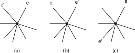
Figure 12: Suppose two edges $e$ and $e^{\prime}$ share a vertex, and there are no other edges between then. This contributes either $1$ or $-1$ depending on the two possibilities (a) and (b). The number $n_{e,e^{\prime}}$ is defined as a sum of all such contributions. Note that (c), with other edges between $e$ and $e^{\prime}$, does not contribute to this computation.

Let us describe the geometrical meaning of the Fock coordinates. For an edge $e$, let us define $l_{e}$ to be the hyperbolic distance between the two punctured connected by the edge $e$. This defines yet another coordinate coordinate of the Teichmüller space, called Penner coordinate or lambda-length [108]. For an edge $e$ as in Figure 11 (a), the relation between the two coordinates are given by

$$Z_{e}=\frac{L_{a}\,L_{c}}{L_{b}\,L_{d}},$$ (A.5)

where we used capitalized letters when we exponentiate variables. For example,

$$L_{e}=e^{l_{e}},\quad Z_{a}=e^{z_{a}}.$$ (A.6)

In other words, Fock coordinate is defined as a cross ratio of Penner coordinates of the four the edges of the quadrilateral.

Another way to explain this is as follows. To explain this, let us represent the Riemann surface on the upper half plane, and the triangles as half-circles having their vertices on the boundary. The uniformization theorem guarantees that by a suitable coordinate transformation this is always possible for Riemann surfaces satisfying (2.3). By a Möbius transformation on the boundary we can choose the vertices of the first triangle to be $0,-1$ and $\infty$. The Fock coordinate $Z$ then coincides with the coordinate of the fourth vertex (Figure 13). This means that Fock coordinates parametrizes the gluing to two triangles.

Figure 13: Fock coordinate determines the gluing to two triangles in the upper half plane. The vertices on the boundary is taken to be $0,-1,\infty$ and $Z$.

Let us describe the change of coordinates under the change of triangulation. For this, it is sufficient to describe the case of the flip as in Figure (11). In Penner coordinates, a flip as in Figure 11 is represented by

$$L_{e}^{\prime}=(L_{a}L_{c}+L_{b}L_{d})/L_{e},$$ (A.7)

while Penner coordinates for all other edges stay the same. This is simply a Ptolemy’s theorem in hyperbolic geometry. Using coordinate transformations in (A.5), this is translated into (assuming the four edges $a,b,c,d$ are all different)

$$\begin{split}Z_{a}^{\prime}=(1+Z_{e})Z_{a},\quad&Z_{b}^{\prime}=(1+Z_{e}^{-1})^{-1}Z_{b},\\ Z_{c}^{\prime}=(1+Z_{e})Z_{c},\quad&Z_{d}^{\prime}=(1+Z_{e}^{-1})^{-1}Z_{d},\\ Z_{e}^{\prime}&=Z_{e}^{-1}.\end{split}$$ (A.8)

More generally, for an edge $f$ different from $e$ we have

$$Z_{f}^{\prime}=(1+Z_{e})^{n_{f,e}}Z_{f}\quad(n_{f,e}\geq 0),\quad\quad Z_{f}^{\prime}=(1+Z_{e}^{-1})^{n_{f,e}}Z_{f}\quad(n_{f,e}<0).\quad$$ (A.9)

We can directly verify that (A.7), (A.8) satisfy the pentagon relation in Figure 11 (b).

Finally, let us proceed to the quantum theory. We choose the quantization in Fock variables. See [21, 25] for quantization in other variables defined by Kashaev, and see [109] the relation between the two quantizations.

The quantization proceeds in the standard way: by replacing the symplectic form by a commutator of operators. For example, in Fock coordinates we have (recall we have $\hbar=2\pi b^{2}$ (2.13))

$$[\mathsf{z}_{e},\mathsf{z}_{e^{\prime}}]=2\pi ib^{2}n_{e,e^{\prime}},$$ (A.10)

or equivalently

$$\mathsf{Z}_{e},\mathsf{Z}_{e^{\prime}}=q^{2n_{e,e^{\prime}}}\mathsf{Z}_{e^{\prime}}\mathsf{Z}_{e},$$ (A.11)

where we defined

$$q=e^{\pi ib^{2}}.$$ (A.12)

The equations for the flip, (A.8), is now modified to be

$$\begin{split}\mathsf{Z}_{a}^{\prime}=(1+q\mathsf{Z}_{e})\mathsf{Z}_{a},\quad&\mathsf{Z}_{b}^{\prime}=(1+q\mathsf{Z}_{e}^{-1})^{-1}\mathsf{Z}_{b},\\ \mathsf{Z}_{c}^{\prime}=(1+q\mathsf{Z}_{e})\mathsf{Z}_{c},\quad&\mathsf{Z}_{d}^{\prime}=(1+q\mathsf{Z}_{e}^{-1})^{-1}\mathsf{Z}_{d},\\ \mathsf{Z}_{e}^{\prime}&=\mathsf{Z}_{e}^{-1}.\end{split}$$ (A.13)

In the classical limit $q\to 1$ this reduces to the classical formula for quantization. We can directly verify that this satisfies the pentagon relation. Moreover, (A.13) preserves the relation (A.10). In fact, under several assumptions this quantization is unique, as has been shown in [110].

A.2 Length Operators

Let us now comment on the construction of the length basis $|l\rangle$ needed for the construction of conformal block (3.20).

For this, let us fix a pants decomposition of $\Sigma$. This means $\Sigma$ can be viewed as a union of trinions (a sphere with 3 holes), and we connect the trinions by a cylinder. For each trinion with the size of holes $l_{i}$ fixed, it is known that there exists a unique metric with negative constant curvature. Moreover, when we glue two trinions together by a cylinder, we can add a twist $\theta_{i}$ along the cylinder circle $C_{i}$ (we call this a pants circle) along the cylinder. We call this twist parameter. The length parameters $l_{i}>0$ and twist parameters $0\leq\theta_{i}<2\pi$ (also called Fenchel-Nielsen coordinates) parametrize the Teichmüller space of the Riemann surface. The important properties of these coordinates is that Weil-Petersson form simplifies in this basis [112]

$$\{l_{i},\theta_{j}\}=\delta_{ij},\quad\{l_{i},l_{j}\}=\{\theta_{i},\theta_{j}\}=0.$$ (A.14)

This provides an important consistency check of the previous proposal that $l$ should be identified with the label for the Virasoro representation (see [19]). The shift of the twist angle $\theta_{i}$ by $\Delta\theta_{i}$ is represented by an operator $e^{i\Delta\theta_{i}l_{i}}$, but this should also be the same as $e^{i\Delta\theta_{i}L_{0}(C_{i})}$, where $L_{0}(C_{i})=\oint_{C_{i}}dzT(z)$ represents the rotation along the circle $C_{i}$. This immediately means $l(C_{i})=L_{0}(C_{i})$.

Let us summarize the classical expression for the geodesic length in terms of Fock coordinates [107]. Let us choose a geodesic $\gamma$ on $\Sigma$ (in the complex structure which is kept fixed in this section). We assume that $\gamma$ does not pass through punctures of $\Sigma$. Then $\gamma$ can be described as a series of segments $\gamma_{i}$, where each $\gamma_{i}$ is a path starting from an edge and ending at another edge of the triangle. Let us denote the Fock coordinate of the edge at the starting point of $\gamma_{i}$ by $z_{i}$. Depending on the two possibilities shown in Figure 14 (a), we define $M_{\gamma_{i}}=VE(z_{i})$ or   or    $M_{\gamma_{i}}=V^{-1}E(z_{i})$, where the matrices $V,E(z)$ are given by

$$V=\left(\begin{array}[]{cc}1&1\\ -1&0\\ \end{array}\right),\quad E(z)=\left(\begin{array}[]{cc}0&e^{z/2}\\ -e^{-z/2}&0\\ \end{array}\right),$$ (A.19)

Then the classical length $l_{\gamma}$ of $\gamma$ is given by the expression

$$L_{\gamma}=2\cosh\frac{l_{\gamma}}{2}=\Big{|}\textrm{Tr}\prod_{i}M_{\gamma_{i}}\Big{|},$$ (A.20)

where the ordering of the product is determined by the ordering of the segments $\gamma_{i}$ inside $\gamma$.

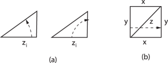
Figure 14: In (a) we list two possibilities for the paths $\gamma_{i}$. In (b) we draw the $\alpha$-cycle on torus, from we read off the classical expression of the geodesic length of the $\alpha$-cycle.

As an example, for once-punctured torus triangulated as in Figure 6, we can choose an $\alpha$-cycle as in Figure 14 (b).

$$L_{\alpha}=\left|\textrm{Tr}\left(V^{-1}E(z)VE(y)\right)\right|=2\cosh\left(\frac{y+z}{2}\right)+\exp\left(\frac{y-z}{2}\right).$$ (A.21)

Quantization of the classical geodesic length $L_{\gamma}$ gives a length operator $\mathcal{L}_{\gamma}$ mentioned in the main text. The length operators for the pants circles $\gamma_{i}$ all commute, since pants circles are non-intersecting. This means that we can simultaneously diagonalize the operators $\mathcal{L}_{\gamma_{i}}$:

$$\mathcal{L}_{i}|l\rangle=2\cosh(2\pi bl_{i})|l\rangle.$$ (A.22)

This is the definition of length basis $|l\rangle$.

For the case of the once-punctured torus, the length operator for the $\alpha$-cycle $\mathcal{L}_{\alpha}$ is the quantization of (A.21)

$$\mathcal{L}_{\alpha}=2\cosh 2\pi b\mathsf{r}+e^{2\pi b\mathsf{s}},$$ (A.23)

see section 4.3 for definitions of $\mathsf{r},\mathsf{s}$ and the their coherent representation $|\mathsf{r}\rangle$. The basis $|l\rangle$ is defined as an eigenstate of the length $L_{\alpha}$.

$$\mathcal{L}_{\alpha}|l\rangle=2\cosh 2\pi bl|l\rangle.$$ (A.24)

Sandwiching (A.23) between $\langle r|$ on the right and $|l\rangle$ on the right, we have a difference equation

$$\langle r-ib|l\rangle=(2\cosh 2\pi bl-2\cosh 2\pi rl)\langle r|l\rangle.$$ (A.25)

From which we derive (up to possible overall normalization factors)

$$\langle r|l\rangle=\frac{s_{b}(l+r+iQ/2)}{s_{b}(l-r-iQ/2)},$$ (A.26)

where we used the property of the quantum dilogarithm (B.8). We can directly verify the completeness relation (3.19) by using an identity of quantum dilogarithms, see [25].

We can also define $|\tilde{l^{\prime}}\rangle$, an eigenstate of the $\beta$-cycle length $\mathcal{L}_{\beta}$. The integral kernel for S-transformation (4.20)is then given by a pairing between the two

$$S_{(l,l^{\prime})}=\langle l|S|l^{\prime}\rangle=\langle l|\tilde{l}^{\prime}\rangle.$$ (A.27)

Appendix B Quantum Dilogarithm

In this appendix we collect formulas for the non-compact quantum dilogarithm function $s_{b}(z)$ and $e_{b}(z)$, which was discovered by Faddeev and his collaborators [63, 64, 8]. See also [113], section III of [114] and an appendix of [115].

The function $s_{b}(z)$ is defined by

$$s_{b}(z)=\exp\left[\frac{1}{i}\int_{0}^{\infty}\frac{dw}{w}\left(\frac{\sin 2zw}{2\sinh(bw)\sinh(w/b)}-\frac{z}{w}\right)\right].$$ (B.1)

In the literature we also find

$$e_{b}(z)=\exp\left(\frac{1}{4}\int_{-\infty+i0}^{\infty+i0}\frac{dw}{w}\frac{e^{-i2zw}}{\sinh(wb)\sinh(w/b)}\right),$$ (B.2)

where the integration contour is chosen above the pole $w=0$. In both these expressions we require $|\mathrm{Im}\,z|<|\mathrm{Im}\,c_{b}|$ for convergence at infinity. There is a simple relation between the two functions

$$e_{b}(z)=e^{\frac{\pi iz^{2}}{2}}e^{-\frac{i\pi(2-Q^{2})}{24}}s_{b}(z),$$ (B.3)

and we loosely refer to both functions as quantum dilogarithms. The relation (B.3) can be shown by decomposing the contour in (B.2) into the three parts $[-\infty,-\epsilon]\cup\epsilon e^{[i\pi,0]}\cup[\epsilon,\infty]$, simplifying expressions, and taking the limit $\epsilon\to 0$. In the classical limit $b\to 0$, we have

$$e_{b}(z)\to\exp\left(\frac{1}{2\pi ib^{2}}\textrm{Li}_{2}(-e^{2\pi bz})\right),$$ (B.4)

where $\textrm{Li}_{2}(z)$ denotes Euler classical dilogarithm function, defined by

$$\textrm{Li}_{2}(z)=-\int_{0}^{z}\frac{\log(1-t)}{t}dt.$$ (B.5)

The quantum dilogarithm function $s_{b}(z)$ has a number of interesting properties. For example, from the definition it follows immediately that

$$s_{b}(z)=s_{1/b}(z).$$ (B.6)

and

$$s_{b}(z)s_{b}(-z)=1.$$ (B.7)

For us, it is important that $s_{b}(z)$ satisfy a difference equation

$$s_{b}\left(z-\frac{ib}{2}\right)=2\cosh\left(\pi bz\right)s_{b}\left(z+\frac{ib}{2}\right),$$ (B.8)

Similarly, for $e_{b}(z)$ we have

$$e_{b}(z-ib^{\pm 1}/2)=(1+e^{2\pi b^{\pm 1}z})e_{b}(z+ib^{\pm 1}/2).$$ (B.9)

We can use these equations to analytically continue $s_{b}(z),e_{b}(z)$ to the whole complex plane. $s_{b}(z)$ is then a meromorphic function with an infinite product expression

$$s_{b}(z)=\prod_{m,n\in\mathbb{Z}_{\geq 0}}\frac{mb+nb^{-1}+\frac{Q}{2}-iz}{mb+nb^{-1}+\frac{Q}{2}+iz}.$$ (B.10)

References

- [1] L. F. Alday, D. Gaiotto, and Y. Tachikawa, Liouville Correlation Functions from Four-dimensional Gauge Theories, Lett. Math. Phys. 91 (2010) 167–197, [arXiv:0906.3219].
- [2] N. Drukker, D. Gaiotto, and J. Gomis, The Virtue of Defects in 4D Gauge Theories and 2D CFTs, arXiv:1003.1112.
- [3] D. Gaiotto, N=2 dualities, arXiv:0904.2715.
- [4] D. Gaiotto and E. Witten, S-Duality of Boundary Conditions In N=4 Super Yang-Mills Theory, arXiv:0807.3720.
- [5] E. Witten, Quantization of chern-simons gauge theory with complex gauge group, Commun. Math. Phys. 137 (1991) 29–66.
- [6] T. Dimofte, S. Gukov, and L. Hollands, Vortex Counting and Lagrangian 3-manifolds, arXiv:1006.0977.
- [7] L. D. Faddeev, R. M. Kashaev, and A. Y. Volkov, Strongly coupled quantum discrete Liouville theory. I. Algebraic approach and duality, Comm. Math. Phys. 219 (2001), no. 1 199–219.
- [8] L. D. Faddeev, Discrete Heisenberg-Weyl group and modular group, Lett. Math. Phys. 34 (1995), no. 3 249–254, [hep-th/9504111].
- [9] L. Faddeev, Modular double of a quantum group, in Conférence Moshé Flato 1999, Vol. I (Dijon), vol. 21 of Math. Phys. Stud., pp. 149–156. Kluwer Acad. Publ., Dordrecht, 2000.
- [10] V. Pestun, Localization of gauge theory on a four-sphere and supersymmetric Wilson loops, arXiv:0712.2824.
- [11] N. A. Nekrasov, Seiberg-Witten Prepotential From Instanton Counting, Adv. Theor. Math. Phys. 7 (2004) 831–864, [hep-th/0206161].
- [12] H. Dorn and H. Otto, Two and three point functions in Liouville theory, Nucl.Phys. B429 (1994) 375–388, [hep-th/9403141].
- [13] A. B. Zamolodchikov and A. B. Zamolodchikov, Structure constants and conformal bootstrap in Liouville field theory, Nucl.Phys. B477 (1996) 577–605, [hep-th/9506136].
- [14] E. P. Verlinde, Fusion Rules and Modular Transformations in 2D Conformal Field Theory, Nucl.Phys. B300 (1988) 360.
- [15] N. Drukker, D. R. Morrison, and T. Okuda, Loop operators and S-duality from curves on Riemann surfaces, JHEP 0909 (2009) 031, [arXiv:0907.2593].
- [16] L. F. Alday, D. Gaiotto, S. Gukov, Y. Tachikawa, and H. Verlinde, Loop and surface operators in N=2 gauge theory and Liouville modular geometry, JHEP 01 (2010) 113, [arXiv:0909.0945].
- [17] N. Drukker, J. Gomis, T. Okuda, and J. Teschner, Gauge Theory Loop Operators and Liouville Theory, JHEP 02 (2010) 057, [arXiv:0909.1105].
- [18] K. Hosomichi, S. Lee, and J. Park, AGT on the S-duality Wall, arXiv:1009.0340.
- [19] H. L. Verlinde, CONFORMAL FIELD THEORY, 2-D QUANTUM GRAVITY AND QUANTIZATION OF TEICHMULLER SPACE, Nucl. Phys. B337 (1990) 652.
- [20] L. Chekhov and V. Fock, Quantum Teichmuller space, Theor.Math.Phys. 120 (1999) 1245–1259, [math/9908165].
- [21] R. M. Kashaev, Quantization of Teichmüller spaces and the quantum dilogarithm, Lett. Math. Phys. 43 (1998), no. 2 105–115.
- [22] J. Teschner, From Liouville theory to the quantum geometry of Riemann surfaces, hep-th/0308031.
- [23] J. Teschner, An analog of a modular functor from quantized Teichmuller theory, math/0510174.
- [24] L. D. Faddeev and R. M. Kashaev, Strongly coupled quantum discrete Liouville theory. II. Geometric interpretation of the evolution operator, J. Phys. A 35 (2002), no. 18 4043–4048.
- [25] R. Kashaev, The quantum dilogarithm and Dehn twists in quantum Teichmüller theory, in Integrable structures of exactly solvable two-dimensional models of quantum field theory (Kiev, 2000), vol. 35 of NATO Sci. Ser. II Math. Phys. Chem., pp. 211–221. Kluwer Acad. Publ., Dordrecht, 2001.
- [26] J. Teschner, Quantization of the Hitchin moduli spaces, Liouville theory, and the geometric Langlands correspondence I, arXiv:1005.2846.
- [27] J. Teschner, Liouville theory revisited, Class.Quant.Grav. 18 (2001) R153–R222, [hep-th/0104158].
- [28] J. Teschner, A Lecture on the Liouville vertex operators, Int.J.Mod.Phys. A19S2 (2004) 436–458, [hep-th/0303150].
- [29] E. Witten, The Central charge in three-dimensions, in Brink, L. (ed.) et al.: Physics and mathematics of strings, pp. 530–559, 1990.
- [30] J. Milnor, On the existence of a connection with curvature zero, Comment. Math. Helv. 32 (1958) 215–223.
- [31] J. W. Wood, Bundles with totally disconnected structure group, Comment. Math. Helv. 46 (1971) 257–273.
- [32] N. J. Hitchin, The self-duality equations on a Riemann surface, Proc. London Math. Soc. (3) 55 (1987), no. 1 59–126.
- [33] H. L. Verlinde and E. P. Verlinde, CONFORMAL FIELD THEORY AND GEOMETRIC QUANTIZATION, based on lectures given at the Trieste Spring School, Apr 1989, and at the Ecole Normale Superieure in Paris, Jun 1989.
- [34] S. Carlip, Inducing Liouville theory from topologically massive gravity, Nucl. Phys. B362 (1991) 111–124.
- [35] E. Witten, Quantum Field Theory and the Jones Polynomial, Commun.Math.Phys. 121 (1989) 351.
- [36] S. Elitzur, G. W. Moore, A. Schwimmer, and N. Seiberg, Remarks on the Canonical Quantization of the Chern-Simons-Witten Theory, Nucl.Phys. B326 (1989) 108.
- [37] A. Alekseev and S. L. Shatashvili, Path Integral Quantization of the Coadjoint Orbits of the Virasoro Group and 2D Gravity, Nucl. Phys. B323 (1989) 719.
- [38] M. Bershadsky and H. Ooguri, Hidden SL(n) Symmetry in Conformal Field Theories, Commun. Math. Phys. 126 (1989) 49.
- [39] P. Forgacs, A. Wipf, J. Balog, L. Feher, and L. O’Raifeartaigh, Liouville and Toda Theories as Conformally Reduced WZNW Theories, Phys.Lett. B227 (1989) 214.
- [40] A. M. Polyakov, Quantum Gravity in Two-Dimensions, Mod.Phys.Lett. A2 (1987) 893.
- [41] O. Coussaert, M. Henneaux, and P. van Driel, The Asymptotic dynamics of three-dimensional Einstein gravity with a negative cosmological constant, Class. Quant. Grav. 12 (1995) 2961–2966, [gr-qc/9506019].
- [42] M. Atiyah, Topological quantum field theories, Inst. Hautes Études Sci. Publ. Math. (1988), no. 68 175–186 (1989).
- [43] N. Nekrasov and E. Witten, The Omega Deformation, Branes, Integrability, and Liouville Theory, arXiv:1002.0888.
- [44] N. A. Nekrasov and S. L. Shatashvili, Quantization of Integrable Systems and Four Dimensional Gauge Theories, arXiv:0908.4052.
- [45] T. Kohno, Topological invariants for -manifolds using representations of mapping class groups. I, Topology 31 (1992), no. 2 203–230.
- [46] E. Witten, Fivebranes and Knots, arXiv:1101.3216.
- [47] O. J. Ganor and Y. P. Hong, Selfduality and Chern-Simons Theory, arXiv:0812.1213.
- [48] O. J. Ganor, Y. P. Hong, and H. Tan, Ground States of S-duality Twisted N=4 Super Yang-Mills Theory, arXiv:1007.3749.
- [49] A. Gadde, E. Pomoni, L. Rastelli, and S. S. Razamat, S-duality and 2d Topological QFT, JHEP 1003 (2010) 032, [arXiv:0910.2225].
- [50] J.-F. Wu and Y. Zhou, From Liouville to Chern-Simons, Alternative Realization of Wilson Loop Operators in AGT Duality, arXiv:0911.1922.
- [51] N. Nekrasov, A. Rosly, and S. Shatashvili, Darboux coordinates, Yang-Yang functional, and gauge theory, arXiv:1103.3919.
- [52] T. Dimofte, From 2d to 3d and Wall Crossing to Chern-Simons, talk at Aspen Center for Physics, August 2010.
- [53] M. Yamazaki and Friends, work in progress.
- [54] V. A. Fateev and A. V. Litvinov, On AGT conjecture, JHEP 02 (2010) 014, [arXiv:0912.0504].
- [55] E. Witten, SL(2,Z) action on three-dimensional conformal field theories with Abelian symmetry, hep-th/0307041.
- [56] K. A. Intriligator and N. Seiberg, Mirror symmetry in three-dimensional gauge theories, Phys.Lett. B387 (1996) 513–519, [hep-th/9607207].
- [57] A. Kapustin, B. Willett, and I. Yaakov, Exact Results for Wilson Loops in Superconformal Chern- Simons Theories with Matter, JHEP 03 (2010) 089, [arXiv:0909.4559].
- [58] D. L. Jafferis, The Exact Superconformal R-Symmetry Extremizes Z, arXiv:1012.3210.
- [59] N. Hama, K. Hosomichi, and S. Lee, Notes on SUSY Gauge Theories on Three-Sphere, arXiv:1012.3512.
- [60] N. Hama, K. Hosomichi, and S. Lee, SUSY Gauge Theories on Squashed Three-Spheres, arXiv:1102.4716.
- [61] T. Okuda and V. Pestun, On the instantons and the hypermultiplet mass of N=2* super Yang-Mills on , arXiv:1004.1222.
- [62] K. Hosomichi, Bulk boundary propagator in Liouville theory on a disc, JHEP 0111 (2001) 044, [hep-th/0108093].
- [63] L. Faddeev and A. Y. Volkov, Abelian current algebra and the Virasoro algebra on the lattice, Phys. Lett. B 315 (1993), no. 3-4 311–318.
- [64] L. D. Faddeev and R. M. Kashaev, Quantum dilogarithm, Modern Phys. Lett. A 9 (1994), no. 5 427–434.
- [65] W. Floyd and A. Hatcher, Incompressible surfaces in punctured-torus bundles, Topology Appl. 13 (1982), no. 3 263–282.
- [66] K. Hikami, Generalized volume conjecture and the -polynomials: the Neumann-Zagier potential function as a classical limit of the partition function, J. Geom. Phys. 57 (2007), no. 9 1895–1940.
- [67] V. G. Turaev and O. Y. Viro, State sum invariants of -manifolds and quantum -symbols, Topology 31 (1992), no. 4 865–902.
- [68] H. Ooguri, Partition functions and topology changing amplitudes in the 3-D lattice gravity of Ponzano and Regge, Nucl.Phys. B382 (1992) 276–304, [hep-th/9112072].
- [69] K. Hikami, Hyperbolic structure arising from a knot invariant, Internat. J. Modern Phys. A 16 (2001), no. 19 3309–3333.
- [70] R. M. Kashaev, Quantum dilogarithm as a -symbol, Modern Phys. Lett. A 9 (1994), no. 40 3757–3768.
- [71] T. Dimofte, S. Gukov, J. Lenells, and D. Zagier, Exact Results for Perturbative Chern-Simons Theory with Complex Gauge Group, Commun. Num. Theor. Phys. 3 (2009) 363–443, [arXiv:0903.2472].
- [72] R. Dijkgraaf, H. Fuji, and M. Manabe, The Volume Conjecture, Perturbative Knot Invariants, and Recursion Relations for Topological Strings, arXiv:1010.4542.
- [73] T. Dimofte, Quantum Riemann Surfaces in Chern-Simons Theory, arXiv:1102.4847.
- [74] Y. Terashima and M. Yamazaki, Semiclassical Analysis of the 3d/3d Relation, arXiv:1106.3066.
- [75] B. Ponsot and J. Teschner, Clebsch-Gordan and Racah-Wigner coefficients for a continuous series of representations of U(q)(sl(2,R)), Commun.Math.Phys. 224 (2001) 613–655, [math/0007097].
- [76] L. Hadasz, Z. Jaskolski, and P. Suchanek, Modular bootstrap in Liouville field theory, Phys.Lett. B685 (2010) 79–85, [arXiv:0911.4296].
- [77] N. Wyllard, conformal Toda field theory correlation functions from conformal N=2 SU(N) quiver gauge theories, JHEP 11 (2009) 002, [arXiv:0907.2189].
- [78] A. Mironov and A. Morozov, On AGT relation in the case of U(3), Nucl.Phys. B825 (2010) 1–37, [arXiv:0908.2569].
- [79] V. Fock and A. Goncharov, Moduli spaces of local systems and higher Teichmüller theory, Publ. Math. Inst. Hautes Études Sci. (2006), no. 103 1–211.
- [80] N. J. Hitchin, Lie groups and Teichmüller space, Topology 31 (1992), no. 3 449–473.
- [81] M. R. Gaberdiel and R. Gopakumar, An Dual for Minimal Model CFTs, arXiv:1011.2986.
- [82] E. Witten, Geometric Langlands From Six Dimensions, arXiv:0905.2720.
- [83] N. Reshetikhin and V. G. Turaev, Invariants of -manifolds via link polynomials and quantum groups, Invent. Math. 103 (1991), no. 3 547–597.
- [84] E. Witten, (2+1)-Dimensional Gravity as an Exactly Soluble System, Nucl. Phys. B311 (1988) 46.
- [85] D. Gaiotto, Asymptotically free N=2 theories and irregular conformal blocks, arXiv:0908.0307.
- [86] A. Marshakov, A. Mironov, and A. Morozov, On non-conformal limit of the AGT relations, Phys. Lett. B682 (2009) 125–129, [arXiv:0909.2052].
- [87] H. Awata and Y. Yamada, Five-dimensional AGT Conjecture and the Deformed Virasoro Algebra, JHEP 01 (2010) 125, [arXiv:0910.4431].
- [88] H. Awata and Y. Yamada, Five-dimensional AGT Relation and the Deformed beta- ensemble, Prog. Theor. Phys. 124 (2010) 227–262, [arXiv:1004.5122].
- [89] A. Stoyanovsky, Quantum Langlands duality and conformal field theory, math/0610974.
- [90] M.-C. Tan, Gauging Spacetime Symmetries on the Worldsheet and the Geometric Langlands Program, JHEP 03 (2008) 033, [arXiv:0710.5796].
- [91] M.-C. Tan, Gauging Spacetime Symmetries On The Worldsheet And The Geometric Langlands Program – II, JHEP 09 (2008) 074, [arXiv:0804.0804].
- [92] E. Frenkel, Lectures on the Langlands program and conformal field theory, in Frontiers in number theory, physics, and geometry. II, pp. 387–533. Springer, Berlin, 2007.
- [93] G. Giribet, Y. Nakayama, and L. Nicolas, Langlands duality in Liouville-H(+)-3 WZNW correspondence, Int.J.Mod.Phys. A24 (2009) 3137–3170, [arXiv:0805.1254].
- [94] M. Kontsevich and Y. Soibelman, Stability structures, motivic Donaldson-Thomas invariants and cluster transformations, arXiv:0811.2435.
- [95] D. Gaiotto, G. W. Moore, and A. Neitzke, Wall-crossing, Hitchin Systems, and the WKB Approximation, arXiv:0907.3987.
- [96] S. Cecotti, A. Neitzke, and C. Vafa, R-Twisting and 4d/2d Correspondences, arXiv:1006.3435.
- [97] G. Bonelli and A. Tanzini, Hitchin systems, N=2 gauge theories and W-gravity, Phys.Lett. B691 (2010) 111–115, [arXiv:0909.4031].
- [98] J. P. Gauntlett, N. Kim, and D. Waldram, M-fivebranes wrapped on supersymmetric cycles, Phys. Rev. D63 (2001) 126001, [hep-th/0012195].
- [99] R. Dijkgraaf and C. Vafa, Toda Theories, Matrix Models, Topological Strings, and N=2 Gauge Systems, arXiv:0909.2453.
- [100] A. Hanany and K. D. Kennaway, Dimer models and toric diagrams, hep-th/0503149.
- [101] S. Franco, A. Hanany, K. D. Kennaway, D. Vegh, and B. Wecht, Brane dimers and quiver gauge theories, JHEP 0601 (2006) 096, [hep-th/0504110].
- [102] S. Franco, A. Hanany, D. Martelli, J. Sparks, D. Vegh, et. al., Gauge theories from toric geometry and brane tilings, JHEP 0601 (2006) 128, [hep-th/0505211].
- [103] B. Szendroi, Non-commutative Donaldson-Thomas theory and the conifold, Geom.Topol. 12 (2008) 1171–1202, [arXiv:0705.3419].
- [104] S. Mozgovoy and M. Reineke, On the noncommutative Donaldson-Thomas invariants arising from brane tilings, arXiv:0809.0117.
- [105] H. Ooguri and M. Yamazaki, Crystal Melting and Toric Calabi-Yau Manifolds, Commun.Math.Phys. 292 (2009) 179–199, [arXiv:0811.2801].
- [106] R. Kenyon and A. Goncharov, work in progress.
- [107] V. V. Fock, Dual Teichmüller spaces, hep-th/9702018.
- [108] R. C. Penner, The decorated Teichmüller space of punctured surfaces, Comm. Math. Phys. 113 (1987), no. 2 299–339.
- [109] R. Guo and X. Liu, Quantum Teichmüller space and Kashaev algebra, Algebr. Geom. Topol. 9 (2009), no. 3 1791–1824.
- [110] H. Bai, A uniqueness property for the quantization of Teichmüller spaces, Geom. Dedicata 128 (2007) 1–16.
- [111] A. Beilinson and V. Drinfeld, Opers, math/0501398.
- [112] S. Wolpert, On the symplectic geometry of deformations of a hyperbolic surface, Ann. of Math. (2) 117 (1983), no. 2 207–234.
- [113] A. Y. Volkov, Noncommutative hypergeometry, Comm. Math. Phys. 258 (2005), no. 2 257–273.
- [114] S. N. M. Ruijsenaars, First order analytic difference equations and integrable quantum systems, J. Math. Phys. 38 (1997), no. 2 1069–1146.
- [115] S. Kharchev, D. Lebedev, and M. Semenov-Tian-Shansky, Unitary representations of , the modular double, and the multiparticle q-deformed Toda chains, Commun. Math. Phys. 225 (2002) 573–609, [hep-th/0102180].