On the Distribution of Orbital Eccentricities for Very Low-Mass Binaries

Abstract

We have compiled a sample of 16 orbits for very low-mass stellar ($<0.1$ $M_{\sun}$) and brown dwarf binaries, including updated orbits for HD 130948BC and LP 415-20AB. This sample enables the first comprehensive study of the eccentricity distribution for such objects. We find that very low-mass binaries span a broad range of eccentricities from near-circular to highly eccentric ($e\approx 0.8$), with a median eccentricity of 0.34. We have examined potential observational biases in this sample, and for visual binaries we show through Monte Carlo simulations that if we choose appropriate selection criteria then all eccentricities are equally represented ($\lesssim 5\%$ difference between input and output eccentricity distributions). The orbits of this sample of very low-mass binaries show some significant differences from their solar-type counterparts. They lack a correlation between orbital period and eccentricity and display a much higher fraction of near-circular orbits ($e<0.1$) than solar-type stars, which together may suggest a different formation mechanism or dynamical history for these two populations. Very low-mass binaries also do not follow the $e^{2}$ distribution of Ambartsumian (1937), which would be expected if their orbits were distributed in phase space according to a function of energy alone (e.g., the Boltzmann distribution). We find that current numerical simulations of very low-mass star formation do not completely reproduce the observed properties of our binary sample. The cluster formation model of Bate (2009a) agrees very well with the overall $e$ distribution, but the lack of any high-$e$ ($>0.6$) binaries at orbital periods comparable to our sample suggests that tidal damping due to gas disks may play too large of a role in the simulations. In contrast, the circumstellar disk fragmentation model of Stamatellos & Whitworth (2009) predicts only high-$e$ binaries and thus is highly inconsistent with our sample. These discrepancies could be explained if multiple formation processes are responsible for producing the field population.

1 Introduction

Binary systems have long been used as unique probes into the origins of stars, as the dynamical imprint of their formation and subsequent evolution are recorded in their orbits. In fact, decades before it was known that nucleosynthesis powers stars, well-determined binary orbits were commonplace (e.g., $>200$ orbits were published in the compilation of Aitken, 1918). Thus, the study of binary orbits has a rich heritage, predating much of modern astrophysics. However, only very recently has it been possible to measure orbits for the lowest mass products of star formation: stars at the bottom of the main-sequence ($<0.1$ $M_{\sun}$) and brown dwarfs. The sample of orbits for such objects has been growing rapidly in recent years as astrometric monitoring has begun to yield orbits for the shortest period visual binaries known ($P\sim 10$ years), which were discovered by high-resolution imaging surveys 5–10 years ago (e.g., Reid et al., 2001, 2006; Bouy et al., 2003; Burgasser et al., 2003, 2006; Close et al., 2003).

Some properties of very low-mass binaries, such as orbital semimajor axes, mass ratios, and multiplicity fractions, can be studied in a statistical fashion using a large sample without any knowledge of orbital motion (e.g., Allen, 2007; Burgasser et al., 2007). However, only well-determined orbits can provide a measure of eccentricity ($e$), which is directly related to the dynamics of the formation process. Because of the long history of stellar orbit studies, many authors have weighed in on the subject of the eccentricity distribution. The most recent comprehensive work on the eccentricities of solar-type field binaries was done by Duquennoy & Mayor (1991), and their pre–main-sequence counterparts have been reviewed by Mathieu (1994). Now for the first time it is possible to bring similar observations to bear on the extreme low-mass end of the binary population. Some of the proposed formation mechanisms for such low-mass objects, such as ejection (e.g., Reipurth & Clarke, 2001) and gravitational instability (e.g., Rice et al., 2003; Stamatellos et al., 2007), may leave a distinct signature in the orbits of binaries. Here we present the first comprehensive look at what orbital eccentricity measurements reveal about the nature of very low-mass stars and brown dwarfs.

2 Updated Orbit Determinations

We first updated published orbit determinations for very low-mass binaries that have new data before compiling our sample for this study. For two visual binaries (HD 130948BC and LP 415-20AB), we present new astrometry from our ongoing Keck adaptive optics (AO) monitoring program in order to refine their orbital elements. Our procedure for obtaining, reducing, and analyzing our natural guide star and laser guide star AO images is described in detail in our previous work (e.g., Dupuy et al., 2009b, c), and the binary parameters derived from our new observations are shown in Table 1. We used the Markov Chain Monte Carlo (MCMC) approach described by Liu et al. (2008) to determine the posterior probability distributions of the orbital elements for these binaries, and in Table 2 we give their median and 68.3% confidence limits. For HD 130948BC, we combined our new astrometry with the epochs published by Dupuy et al. (2009b). We updated this astrometry to account for the newer astrometric calibration of NIRC2 by Ghez et al. (2008), which amounts to a $+0\fdg 26$ offset to our previously published position angles. The extended orbital phase coverage results in a factor of $\approx$4 improvement in precision compared to the published orbital parameters.

Some binaries have multiple orbit determinations in the literature, and in these cases we used our published results in the following analysis. In most cases published orbits are in good agreement with each other, but a few binaries warrant special mention. In the case of LP 415-20AB, our astrometry results in a very different orbit than found by Konopacky et al. (2010). As a test, we fitted their three Keck epochs with the published Gemini epoch from Siegler et al. (2003) and found an orbit consistent with the one they reported ($e=0.9\pm 0.1$). However, after including our four Keck epochs we found that the 2007 December astrometry of Konopacky et al. (2010) is highly discrepant with the ensemble of measurements, resulting in a $\chi^{2}$ of 21.5 for 9 degrees of freedom (DOF). If we exclude this one measurement, we find good agreement between the data sets, and the best-fit orbit has a reasonable $\chi^{2}$ (6.83 for 7 DOF) and significantly different orbital parameters (e.g., our newly derived eccentricity of $0.708^{+0.014}_{-0.016}$ is 1.9$\sigma$ discrepant with their $0.9\pm 0.1$). It appears that with only four epochs (i.e., 1 DOF) the orbit fit of Konopacky et al. (2010) was vulnerable to a single discrepant astrometric measurement leading to an incorrect orbit solution. We also note that our published orbit for 2MASS J2206$-$2047AB (Dupuy et al., 2009a) is nominally inconsistent with that published by Konopacky et al. (2010), with all orbital parameters discrepant by $\approx$2–4$\sigma$. Using only their data, we have found a lower $\chi^{2}$ orbit solution than they report, and although it is more consistent with our published orbit, it still has an unrealistically large $\chi^{2}$ (30.3 for 9 DOF). Thus, we choose to use our published orbit for 2MASS J2206$-$2047AB ($\chi^{2}=7.49$ for 7 DOF) in the following analysis. Finally, the orbit for 2MASS J1534$-$2962AB published by Konopacky et al. (2010) is marginally inconsistent with the original orbit from Liu et al. (2008). With the latest astrometry the period and semimajor axis are smaller by 1.8$\sigma$, while the eccentricity and mass are consistent within 1$\sigma$. We use the more recent orbit from Konopacky et al. (2010) in the following analysis.

3 Very Low-Mass Binary Sample

We have constructed a sample of very low-mass ($\mbox{$M_{\rm tot}$}<0.2$ $M_{\sun}$) binary orbits, including both visual and spectroscopic binaries. Because it is imperative for our purposes that this sample be as unbiased as possible with respect to eccentricity, in the following analysis we consider potential sources of selection bias, the nature of which varies between different types of binaries. Below we describe how we have selected our orbit sample as well as the tests we have performed to quantify the level of eccentricity bias present in this sample.

3.1 Visual Binaries

In Table On the Distribution of Orbital Eccentricities for Very Low-Mass Binaries, we present a list of all 20 visual binaries that have published orbit determinations and a total system mass $<0.2$ $M_{\sun}$. For each binary we list its distance, semimajor axis ($a$), and eccentricity ($e$), as these are the physical parameters that, along with three viewing angle parameters, determine the size and shape of a binary’s orbit on the sky. Thus, these are the three key parameters that must be considered when characterizing selection biases. In most cases we have used orbit parameters as published and distances determined from trigonometric parallax measurements. When parallax measurements were not available, we estimated distances based on the primary components’ resolved photometry and spectral types using the updated spectral type–absolute magnitude relations described in Appendix B of Liu et al. (2010).

For all orbits published by other authors, we have created our own Markov chains using the published astrometry and the same analysis method described in Section 2. However, only in the cases where the astrometric orbit fits yield a reasonable $\chi^{2}$ can we trust the MCMC analysis to provide accurate posterior distributions of the orbital parameters. In cases where $\chi^{2}$ is unreasonably large, the parameter space is not fully explored and uncertainties can be significantly underestimated by the MCMC method (or in fact by any fitting method). We find such large $\chi^{2}$ values (reduced $\chi^{2}=2.8$–120) for five of the orbits published by Konopacky et al. (2010). For three of these orbits they combined astrometry with radial velocities (2MASS J1847$+$5522AB, 2MASS J1750$+$4424AB, 2MASS J1426$+$1557AB), which may have enabled them to achieve orbit fits with smaller $\chi^{2}$ than we found using the astrometry alone. For the other two orbits (2MASS J0850$+$1057AB and 2MASS J1728$+$3948AB), it is unclear why we are unable to reproduce their lower $\chi^{2}$ values from the same input data (astrometry alone). For all five of these orbits we use the parameters derived by Konopacky et al. (2010). (Note that for reasons unrelated these discrepancies, none of these five binaries ultimately passes the selection criteria that we define below for our unbiased eccentricity sample.)

3.1.1 Selecting a Minimally Biased Sample

With a complete set of the known very low-mass visual binary orbits in hand, we now consider how selection biases may affect the eccentricity distribution of this sample. Visual binaries must pass three independent selection criteria before having their orbits determined: (1) they must be initially resolved by a high-resolution imaging survey; (2) they must be included in subsequent astrometric monitoring programs; and (3) their observed relative motion must yield a unique orbit fit. The first selection cut can result in biases on orbital parameters, as has been shown for direct imaging searches for extrasolar planets (e.g., see Brown, 2004). The second cut results from the fact that it is impractical to monitor the orbits of all $\approx$100 known very low-mass binaries. Rather, astrometric monitoring programs are inevitably optimized for measuring as many orbits as possible with limited observing resources over a limited amount of time by focusing on the binaries likely to have the shortest orbital periods. Thus, the selection criteria used to define the monitoring sample can result in strong biases on the orbit parameters. Because the orbital period must be estimated from the projected separation of the binary, binaries with wide separations are much less desirable to monitor. This introduces an eccentricity bias because more eccentric binaries at a given period and mass will, on average, have wider projected separations. We will therefore attempt to define a subset of visual binaries that has minimal eccentricity bias due to these selection criteria.

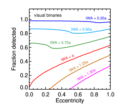
Figure 1: Top: Fraction of visual binaries detected in Monte Carlo simulations of a single-epoch imaging survey, where the input eccentricity distribution is uniform. Different colored lines show simulations in which the semimajor axis ($a$) was fixed at different multiples of the resolution limit, or inner working angle (IWA). When the semimajor axis lies inside the IWA highly eccentric orbits are strongly preferred, and as the IWA goes to zero the eccentricity bias disappears. Bottom: Eccentricity bias for binaries with late-M (solid) and L dwarf (dashed) primaries as determined from Monte Carlo simulations assuming a magnitude-limited sample with semimajor axis drawn from the log-normal Allen (2007) distribution. The resolution limit for both simulations was chosen to be the worst-case from among all surveys that discovered the binaries in our sample (0$\farcs$12 for late-M dwarfs and 0$\farcs$07 for L dwarfs). The resulting worst-case eccentricity bias is modest, only slightly ($\approx$5%) favoring the discovery of highly eccentric ($e>0.8$) and nearly circular ($e<0.2$) binaries.

$\bullet$ Discovery bias. We first consider the effect of “discovery bias” which causes the population of binaries resolved by imaging surveys to deviate from the true underlying eccentricity distribution of all binaries. For a given imaging surveys, the extent of this bias depends on how the semimajor axis ($a$) distribution compares to that survey’s resolution limit, or inner working angle (IWA). For example, if the $a$ distribution peaks inside the IWA, the discovery of higher eccentricity binaries is favored, as such binaries spend more time at wider separations compared to more circular orbits. To quantify this bias, we have performed a simple Monte Carlo simulation in which $a$ was held fixed, while eccentricity was distributed uniformly from 0 to 1, viewing angles were drawn from appropriate random distributions ($p(i)\propto\sin{i}$; uniform in $\omega$ and $\Omega$), and the single-epoch observations were distributed uniformly in orbital phase. Binaries were considered detected if their projected separation at the time of observation was above the resolution limit. The impact on the uniform input eccentricity distribution is illustrated in Figure 1. When the resolution limit falls at or outside the fixed semimajor axis (IWA $\geq~{}a$), high-$e$ orbits are strongly preferred as they spend the most time wider than the resolution limit. When the resolution limit falls inside the fixed value of $a$ (IWA $<a$) both highly eccentric and circular orbits are preferred, with intermediate eccentricities being selected against. This is because in these cases any sufficiently eccentric orbit can be made unresolvable by an unfavorable viewing angle, but this can be compensated by the fact that the most eccentric orbits spend extended periods of time at very wide separations. Thus, high-$e$ orbits are more likely to be detected than intermediate-$e$ orbits, as they spend the most time widely separated.

To predict the exact form of the eccentricity discovery bias for our sample would require an assumption for the underlying semimajor axis distribution as well as careful accounting of the resolution limits of the numerous imaging surveys that have contributed to the current sample of very low-mass binaries. However, for our purposes we simply want to ensure that our sample of orbits has an acceptably small amount of bias. Thus, we need only chose a cutoff in the ratio of IWA/$a$ that is small enough to minimize the bias while including as many binaries with orbit determinations as possible. In Table On the Distribution of Orbital Eccentricities for Very Low-Mass Binaries, we give our estimate for the IWA of the imaging data used to discover each visual binary as well as the ratio IWA/$a$. We have chosen a cutoff of IWA/$a<0.75$, which Figure 1 shows produces a relatively unbiased selection over a full range of eccentricities from 0 to 1. This cutoff excludes three binaries: LP 415-20AB (IWA/$a\approx 1.28$), 2MASS J0920$+$3517AB (IWA/$a\approx 0.91$), and 2MASS J2140$+$1625AB (IWA/$a\approx 0.83$). The highest remaining IWA/$a$ value in our sample is 0.68 for LP 349-25AB. While it is unfortunate to have to exclude any orbits from our sample, we emphasize that this is a very important step in keeping potentially large biases from impacting the following analysis. The case of LP 415-20AB is a prime example of the problem with discovery bias on eccentricity. This binary was discovered at a projected separation of $119\pm 8$ mas, right at the resolution limit of the imaging survey of Siegler et al. (2003). Its actual semimajor axis turns out to be $93.5^{+3.1}_{-2.3}$ mas, so it could have only been discovered by that survey if it had an eccentric orbit, as it indeed does ($e=0.708^{+0.016}_{-0.014}$). Thus, while LP 415-20AB does tell us that very low-mass binaries can be quite eccentric, it cannot convey any other information about the eccentricity distribution since the only reason it was discovered is because of its large eccentricity.

$\bullet$ Monitoring sample bias. Next, we consider how to prevent the sample selection of orbital monitoring programs from biasing the resulting eccentricity distribution. This is essentially a matter of choosing a range of semimajor axes for which the monitoring sample is complete at all eccentricities. The lower limit in $a$ is simply defined by the visual binary orbit with the smallest semimajor axis; this is Gl 569Bab with $a=0.923\pm 0.018$ AU (Dupuy et al., 2010). There are also no known visual binaries with projected separations ($\rho$) at discovery smaller than 0.9 AU, so we define this as the lower limit of our sample. The upper limit should be chosen to accurately reflect the completeness of orbit monitoring surveys that tend to focus on the smallest separation binaries, while also including as many of the resulting orbit measurements as possible. For the many binaries without orbit determinations, we must use their minimum possible semimajor axis, which would be the case of a highly eccentric, face-on orbit caught at apoastron (physical separation of $a(1+e)$). Since bound orbits have $0<e<1$, the minimum possible semimajor axis for any binary is therefore half its projected separation ($\rho/2$). Thus, some binaries that seem to be very wide (i.e., poor monitoring targets) could in fact have much smaller semimajor axes but just be very eccentric. When choosing an upper limit in $a$, we must therefore ensure that orbit monitoring programs are complete up to projected separations of $2a$, otherwise we would introduce a strong selection bias against high eccentricities. We choose an upper limit in $a$ of 3.7 AU in order to include the binaries LHS 1070BC ($3.57\pm 0.07$ AU; Seifahrt et al., 2008) and LHS 1901AB ($3.70\pm 0.16$ AU; Dupuy et al., 2010). The next widest binary that would also pass our IWA/$a$ cut is 2MASS 0850$+$1057AB ($4.8^{+3.9}_{-1.4}$ AU, $e=0.64\pm 0.26$). Our chosen 3.7 AU upper limit means that binaries up to projected separations of 7.4 AU should not have been intentionally excluded from orbit monitoring programs. To the best of our knowledge this is the case, as at least a second epoch has been obtained for all binaries with $\rho<7.4$ AU, either by our own Keck program or others (e.g., Bouy et al., 2008; Konopacky et al., 2010). A slightly larger upper limit of 4.0 AU would require several more binaries to have undergone orbit monitoring that have not, while adding no additional binaries with orbit determinations to our sample.

$\bullet$ Monte Carlo simulations. With these selection criteria of $0.9<a<3.7$ AU, $\rho<7.4$ AU, and IWA$/a<0.75$ in hand, we have performed Monte Carlo simulations to assess the level of eccentricity bias that is expected for our sample. For this range of semimajor axes, the very low-mass binary parameter distributions derived by Allen (2007) are appropriate. The semimajor axis distribution is lognormal, with a peak at $\log(a/{\rm AU})=0.86$ and $\sigma_{\log{a}}=0.28$. To convert $a$ from AU to arcseconds, we randomly drew distances in a Monte Carlo fashion incorporating the selection effects of the seeing-limited surveys that originally discovered the binaries as unresolved sources. We began with objects distributed uniformly in volume. We assigned magnitudes to these objects according to the empirical $K_{S}$-band luminosity function of Cruz et al. (2007) which is valid from $9.5<M_{\mbox{$K_{S}$}}<13.0$ mag (i.e., $\approx$M8 to L8, encompassing the spectral type range of the bulk of our sample). We further added flux due to unresolved companions according to the Allen (2007) binary frequency of 20% and mass ratio distribution of $q^{1.8}$; we converted mass ratio to flux ratio using the $L\propto M^{2.4}$ theoretical power-law relation of Burrows et al. (2001). The final distance distribution was then determined by magnitude cuts on this simulated population. We tested both strong ($\mbox{$K_{S}$}<12.0$ mag) and weak ($\mbox{$K_{S}$}<15.0$ mag) magnitude cuts equivalent to those used by Gizis et al. (2000) and Kirkpatrick et al. (2000) in mining 2MASS for late-M dwarfs and L dwarfs, respectively. In the latter case, we applied an additional $M_{\mbox{$K_{S}$}}>11.0$ mag cut to approximate the $J-K>1.7$ mag color cut of Kirkpatrick et al. (2000) that excluded brighter, bluer M dwarfs; we based this cut on the color–absolute magnitude diagrams of Dahn et al. (2002).

The strong magnitude cut for the brighter late-M sample resulted in a distance distribution peaking at $\approx$20 pc, while the weaker cut for the fainter L dwarf sample resulted in similarly shaped distribution peaked at $\approx$40 pc. We then randomly generated an observed projected separation ($\rho$) for each binary in a similar manner as described earlier (i.e., random viewing angles and observing times, and a uniform eccentricity distribution). Figure 1 shows the resulting eccentricity distribution after applying the selection criteria of $0.9<a<3.7$ AU, IWA$/a<0.75$, $\rho<7.4$ AU, and $\rho>{\rm IWA}$ (i.e., the binary was resolved). For both samples we conservatively assumed the worst-case IWA from the surveys that originally discovered the binaries in our sample. For the late-M dwarfs this is 0$\farcs$12 from the Gemini AO surveys (e.g., Close et al., 2002, 2003; Siegler et al., 2003), and for the L dwarfs this is 0$\farcs$07 from both HST and Keck surveys (e.g., Bouy et al., 2003; Reid et al., 2006; Siegler et al., 2007). By assuming the worst-case IWA we find the largest possible amplitude of the eccentricity bias, since smaller values of the IWA will always yield less bias (i.e., more binaries will always be uncovered for a smaller IWA). The resulting maximal bias we find from our Monte Carlo simulations has an amplitude of less than $\pm 5\%$ for both the late-M and L samples. As expected, the level of eccentricity bias introduced by our selection criteria is negligible, since they were chosen to minimize the eccentricity bias, and as shown in Figure 1 there is no strong systematic trend in the bias. Nearly circular ($e<0.2$) and highly eccentric orbits ($e>0.8$) are slightly preferred (by $\approx$4%) as compared to intermediate eccentricities. We neglect this bias in the following analysis.

$\bullet$ Orbit fitting bias. Finally, we consider one additional selection effect present in our sample: each binary must have undergone astrometric motion suitable for yielding a robust orbit determination. This can potentially introduce an eccentricity bias if orbit fits are more easily determined for certain ranges of eccentricity. For example, it is easy to imagine that an extremely eccentric binary would present a challenge to astrometric monitoring as it spends most of its time at a fixed projected separation before moving rapidly inward in nearly a straight line. Such an orbit would be difficult to observe at just the right times needed for a good fit and would also appear to be less appealing for continued monitoring. Harrington & Miranian (1977) investigated this bias by generating $10^{3}$ random orbits and classifying the expected quality of the orbit fit by eye, relying on their extensive experience working with such astrometric data. Such an ad hoc method is necessary because in the marginal cases of visual binary orbit fitting the process of $\chi^{2}$ minimization is highly nonlinear and strongly dependent on the initial guess. Harrington & Miranian (1977) found that on average orbits with $e<0.6$ all had the same likelihood of yielding a good fit, so they assigned this eccentricity range a normalized completeness factor of 100%. They found that this completeness drops to 77% for eccentricities of 0.6–0.8 and 42% for $e>0.8$. In our sample, we have one visual binary with $e>0.8$ and none in the 0.6–0.8 range. In the following analysis we consider the impact of applying correction factors of 1.3$\times$ and 2.4$\times$ due to this orbit fitting bias.

$\bullet$ Final visual binary sample. In Table On the Distribution of Orbital Eccentricities for Very Low-Mass Binaries, we list the orbital periods, eccentricities, and masses of the eleven visual binary orbits from Table On the Distribution of Orbital Eccentricities for Very Low-Mass Binaries that meet our eccentricity bias-minimizing criteria of having $0.9<a<3.7$ AU and a discovery IWA$/a<0.75$. (Note that we list orbital period here rather than semimajor axis in order to compare these orbits directly to the unresolved spectroscopic binary orbits.) Although this nominally includes only a little over half of the 20 published visual binary orbit determinations, in fact the majority of the remaining orbits would not contribute much information as they are not as well constrained (see the orbit quality metrics given in Table On the Distribution of Orbital Eccentricities for Very Low-Mass Binaries). For example, all orbits in our bias-minimized sample happen to have 1$\sigma$ eccentricity confidence limits of $\lesssim 0.1$ (median 0.005). However, of the nine orbits not included in the sample, six of them have much more poorly constrained orbits (1$\sigma$ confidence limits of 0.1–0.5), with a median error of 0.26 that is $>50\times$ larger than the median for the other orbits. In fact, the reason why these six orbits are poorly determined is the same as why they were excluded by our bias minimizing criteria: they are all the widest (i.e., longest period) binaries, and this results in them having orbit monitoring observations that cover much less orbital phase (as little as 0.2% and 1.3% of the orbit is covered in the two most extreme cases).

3.2 Spectroscopic Binaries

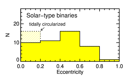
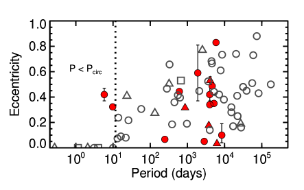
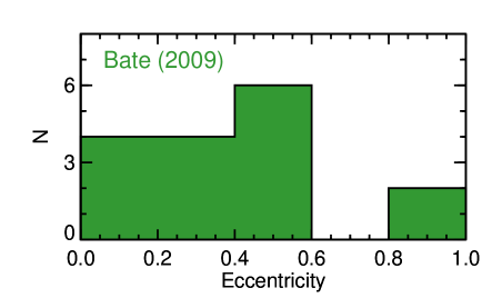
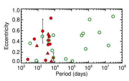
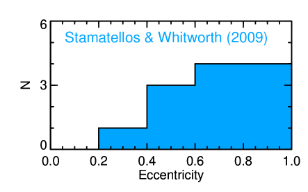
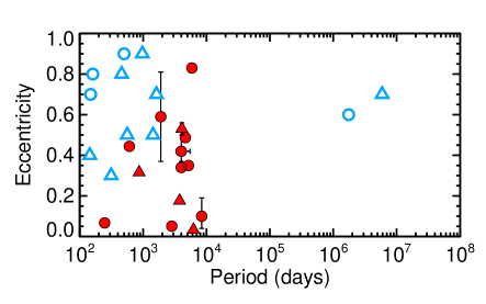
Figure 4: Eccentricity distributions (left) and orbital period–eccentricity diagrams (right, open symbols) for various samples. Top: Solar-type binaries from Duquennoy & Mayor (1991), with three low-quality, $>$1000-yr orbits excluded. Tidally circularized orbits ($P<\mbox{$P_{\rm circ}$}$) are plotted separately in the histogram (hatched region). Triangles and squares denote members of hierarchical triple and quadruple systems, respectively. Middle: Cluster formation model simulated binaries from Bate (2009a); eccentricities for this sample of very low-mass simulated binaries are reported by Bate (2010). Bottom: Circumstellar disk fragmentation model simulated binaries from Stamatellos & Whitworth (2009), with triangles denoting binaries that remain bound to the simulated host star. The very low-mass binaries in our sample are shown as filled red symbols on all $P$–$e$ diagrams for comparison.

To date, five unresolved very low-mass binaries have published orbit determinations. Two of these were discovered via radial velocity (RV) monitoring as single-lined spectroscopic binaries (SB1s): Cha H$\alpha$ 8 ($e=0.59\pm 0.22$; Joergens & Müller, 2007), and 2MASS J0320$-$0446 ($e=0.067\pm 0.015$; Blake et al., 2008). Shen & Turner (2008) have examined the selection bias introduced by RV surveys on the eccentricity distribution through Monte Carlo simulations. They found that as long as the RV semiamplitude ($K_{1}$) of an SB1 is $\gtrsim$3$\times$ larger than the rms of the residuals ($\sigma$), its eccentricity does not greatly impact its likelihood of discovery. As shown in their Figure 4, SB1s have a constant detection efficiency up to $e=0.6$, beyond which there is a slight downturn. However, even at the highest eccentricities ($0.85<e<1.0$) the detection efficiency is only $\approx$20% less than for $e<0.6$ orbits. The reason for this lack of a strong eccentricity bias in RV data is because eccentricity acts to boost the RV semiamplitude ($K_{1}\propto 1/\sqrt{1-e^{2}}$), counteracting the fact that eccentric orbits are more difficult to adequately sample with times series data. The two SB1s in our sample, Cha H$\alpha$ 8 and 2MASS J0320$-$0446, have large semiamplitudes relative to their rms ($K_{1}/\sigma=11$ and 21, respectively), and thus are expected to harbor little bias ($<20\%$) with respect to eccentricity according to the analysis of Shen & Turner (2008). For this reason and the small size of the sample (2 systems) we neglect the eccentricity bias for SB1s.

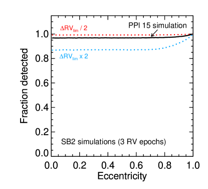
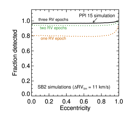
Figure 2: Top: Fraction of SB2s detected in Monte Carlo simulations of a three-epoch RV survey, where the input eccentricity distribution is uniform. The solid black line is a simulation designed to imitate the case of PPl 15, the only SB2 in our orbit sample. Dotted colored lines show simulations in which the detection threshold ($\Delta{\rm RV}=11$ km s^-1) was changed by a factor of two. The RV observations that discovered PPl 15 only slightly ($\approx$3%) favored the detection of highly eccentric ($e\gtrsim 0.8$) binaries. This effect would be larger ($\approx$15%) for binaries with a factor of two lower RV semiamplitudes. Bottom: Same as top panel, except that the dotted colored lines show variations in the eccentricity bias due to having fewer than the three epochs of RV data that were available for the detection of PPl 15. Surveys with only one or two RV epochs are less sensitive to SB2s at all eccentricities, and they are more biased toward the discovery of highly eccentric binaries.

One double-lined spectroscopic binary (SB2) has a measured orbit: PPl 15 ($e=0.42\pm 0.05$ Basri & Martín, 1999). It was discovered as an SB2 in three epochs of RV data. The identification of SB2s in spectroscopic data is subject to different eccentricity selection effects than for SB1s because changes in the velocity do not need to be measured to detect the two sets of absorption lines due to the binary. To quantify the eccentricity bias in detecting SB2s, we performed a Monte Carlo simulation similar to the one described above for visual binaries but with the detection criterion that the velocity shift between the binary components must be large enough to detect in high-resolution spectra at one of three random epochs. We fixed the period and semimajor axis to that of PPl 15 (5.8 days, 0.03 AU). Figure 2 shows the resulting SB2 eccentricity bias predicted by our simulation for a detection threshold of $\Delta{\rm RV}=11$ km s^-1 (i.e., 3$\times$ the spectral resolution of Basri & Martín, 1999). We find only a slight ($\approx$3%) preference for the discovery of highly eccentric ($e>0.8$) SB2s in such RV data. For comparison, we also show the results if the detection threshold were higher or lower by a factor of two, as would be the case for binaries with RV semiamplitudes different by a factor of two. Higher semiamplitude binaries are less biased, while for lower semiamplitudes the eccentricity bias becomes a larger effect (though still $\lesssim 15\%$). Thus, it seems reasonable to neglect eccentricity bias for PPl 15, the one SB2 in our orbit sample.

LSR J1610$-$0040 ($e=0.444\pm 0.017$) is the only very low-mass astrometric binary known to date, discovered by the USNO parallax program (Dahn et al., 2008). It was later found to be an SB1 in the multi-epoch RV data obtained by Blake et al. (2010). In principle, astrometric time series data is very similar to RV time series data and so would be subject to the same biases as for SB1s. Thus, we assume that the same selection effects apply, namely that orbits with $e>0.85$ have an $\approx$80% detection efficiency relative to less eccentric orbits, which are all equally accessible by astrometric monitoring.

Finally, just one very low-mass eclipsing binary is known, 2MASS J0535$-$0546 ($e=0.323\pm 0.006$), discovered by Stassun et al. (2006) in a photometric variability survey. In a study of exoplanet transit surveys, Burke (2008) showed that photometric transit/eclipse detections are only slightly biased ($<10\%$) in eccentricity, with the exact correction depending on the underlying $e$ distribution. Thus, we neglect any eccentricity bias for 2MASS J0535$-$0546.

Table On the Distribution of Orbital Eccentricities for Very Low-Mass Binaries lists the orbital periods, eccentricities, and masses for these five unresolved binaries’ orbits. Combined with the visual binary sample, our sample comprises a total of 16 very low-mass binary orbits spanning orbital periods from 5.8 days to 8400 days.

4 Discussion

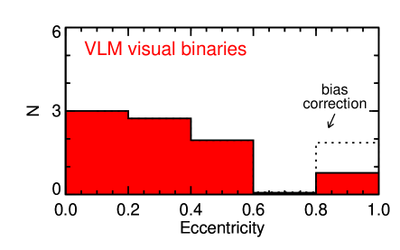
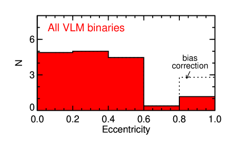
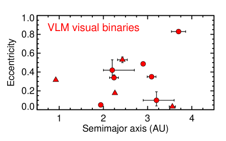
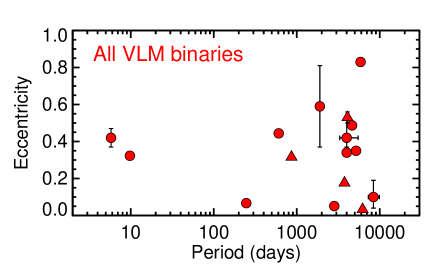
Figure 3: Top: Eccentricity distributions for our sample of eleven very low-mass visual binaries (left) and the full sample including spectroscopic binaries (right). The dotted histograms show the orbit-fitting bias correction we applied to visual binaries in the last two bins ($e>0.6$). Histograms were generated from $10^{4}$ randomly drawn eccentricity values for each binary corresponding to the measurement error, so some bins may have a non-integer value. Bottom: Eccentricity plotted as a function of semimajor axis for the visual binary sample (left) and as a function of orbital period for the full sample including spectroscopic binaries (right). Triangles denote members of hierarchical triple systems, and circles denote true binaries.

The eccentricity distribution and orbital period–eccentricity diagram for our sample is shown in Figure 3. Our sample shows a strong preference for modest eccentricities, with a median eccentricity of 0.34 (mean also 0.34) for the full sample and a median of 0.33 (mean of 0.33) for the visual binaries alone. The visual binary orbits show a broad range of eccentricities, from near-circular up to $e=0.830$. At the shortest periods ($P\lesssim 1000$ days), we find an absence of eccentric orbits ($e>0.5$), although this could be due to small number statistics. Thus, we find no strong evidence that the eccentricity distribution of very low-mass binaries changes over three orders of magnitude in orbital period ($6<P<8\times 10^{3}$ days).

We have quantified the lack of a correlation between period and eccentricity by computing Spearman’s rank correlation coefficient ($r_{S}$) for our sample. We use a Monte Carlo approach, accounting for the period and eccentricity errors by drawing the data in each trial from the observed distributions (our MCMC chains when possible, Gaussians otherwise). The resulting mean and rms of the correlation coefficient was $r_{S}=-0.02\pm 0.07$, which is well below the critical value of 0.412 needed to show correlation for our sample even at 90% confidence. The subset of visual binaries also shows no significant $P$–$e$ correlation ($r_{S}=0.02\pm 0.08$, critical value 0.497 at 90% confidence) or $a$–$e$ correlation ($r_{S}=0.14\pm 0.09$). In contrast, Konopacky et al. (2010) reported a trend in $e$ as a function of period for their sample of fifteen very low-mass visual binaries, although they did not quantify the significance of the correlation. We note that their observed trend is largely dependent on the two longest period orbits in their sample ($P=320\pm 240$ yr and $2000^{+2100}_{-1900}$ yr) for which they found large eccentricities with large errors ($e=0.71\pm 0.18$ and $0.85^{+0.10}_{-0.41}$, respectively). Both of these binaries were excluded from our sample by our criteria for minimizing eccentricity bias, and we also note that with only 2.2% and 0.4% observational phase coverage these orbit determinations and their uncertainties are not likely to be robust (e.g., see the cautionary example of DF Tau AB in Schaefer et al., 2006).

We have also investigated whether mass ratio is correlated with eccentricity for our sample. In Table On the Distribution of Orbital Eccentricities for Very Low-Mass Binaries, we list the best available mass ratio ($q\equiv M_{2}/M_{1}$) estimates or measurements for our sample binaries. For the visual binaries, $q$ is estimated from Lyon evolutionary models (Chabrier et al., 2000; Baraffe et al., 2003) given the measured total mass and individual luminosities using the method described in Section 5.4 of Dupuy et al. (2009b). This has been done in a consistent fashion for the sample presented here, so even if there are systematic errors in the evolutionary models the relative ordering of the mass ratios should be relatively unaffected. For the eclipsing binary 2MASS J0535$-$0546, we used its directly measured mass ratio ($0.64\pm 0.04$; Stassun et al., 2006). None of the three SB1s in our sample has a well-determined mass ratio, so we excluded them from our mass ratio analysis. We also excluded one visual binary (LHS 2397aAB) because it has a very large uncertainty in its mass ratio estimate ($0.71^{+0.09}_{-0.14}$; Dupuy et al., 2009c) due to the fact that it is composed of a main-sequence star and a field brown dwarf. We computed Spearman’s rank correlation coefficient in a Monte Carlo fashion as described above and found $r_{S}=-0.09\pm 0.10$, showing that there is no evidence for a correlation of eccentricity with mass ratio over the range of our sample ($0.6\lesssim q\lesssim 1.0$). In the absence of such a correlation, any mass ratio selection effects present in our sample should therefore not induce a systematic eccentricity bias.

4.1 Comparison to Solar-type Binaries

Duquennoy & Mayor (1991) have examined in detail the eccentricity distribution of a well-defined sample of solar-type binaries. In the following analysis, we exclude from consideration three of the binaries in their sample that have an orbit quality grade of 4 or 5 assigned by Worley & Heintz (1983), which indicates an indeterminate orbit. Not surprisingly, these binaries (HD 16895AB, HD 78154AB, and HD 146361AB) are the longest period orbits in the Duquennoy & Mayor (1991) sample, with orbital periods $>1000$ yr. (We note that Raghavan et al. (2010) have recently updated this volume-limited, solar-type sample, but we cannot use this for comparison since they did not publish the eccentricity values of their sample binaries.)

We find that the overall eccentricity distribution of the Duquennoy & Mayor (1991) solar-type binary sample is very similar to our orbit sample. To assess this quantitatively, we performed Kolmogorov-Smirnov (KS) tests in a Monte Carlo fashion. We accounted for eccentricity errors in our sample by drawing the data in each trial from the observed distributions (our MCMC chains when possible, Gaussians otherwise). We computed the KS statistic ($D$) and the corresponding probability for every trial. The resulting rms scatter in $D$ was relatively small($\leq 0.05$). For the final probability that two samples were drawn from the same parent distribution, we used the mean of the probabilities from individual trials. Table 5 shows the resulting probabilities comparing subsamples of our orbits to subsamples of the solar-type binaries from Duquennoy & Mayor (1991). In general, we find good agreement between the two samples’ eccentricity distributions. However, a more detailed examination of these samples shows some significant differences.

Unlike the very low-mass binaries, solar-type binaries follow a strong correlation with orbital period such that short-period ($<10^{3}$ days) binaries span a different range of eccentricities than do long-period ($>10^{3}$ days) binaries (Figure 4). Duquennoy & Mayor (1991) suggested that this implies a different formation mechanism and/or dynamical history for these two period regimes of solar-type binaries. The same trend has also been reported for pre–main-sequence, solar-type binaries (Mathieu, 1994, and references therein), implying that this period–eccentricity correlation is determined early in a binary’s formation history. We confirm the significance of the correlation in the Duquennoy & Mayor (1991) sample by computing Spearman’s rank correlation coefficient for solar-type binaries (excluding those that lie below the critical period for tidal circularization; $\mbox{$P_{\rm circ}$}=11.6$ days). The resulting value of $r_{S}=0.32$ for this sample of 46 solar-type binaries gives a 98.6% confidence that $P$ and $e$ are correlated. As discussed above, our sample shows no such correlation, which is an indication that the solar and very low-mass populations are in fact dynamically distinct from one another.

We also note that among the large sample of solar-type binaries from Duquennoy & Mayor (1991) there is not a single orbit with $e<0.1$ beyond an orbital period of 22 days, while there are at least 3 such orbits in our sample of 16 binaries (one more, 2MASS J1534$-$2952AB, could also have $e<0.1$, but the error in its eccentricity makes this uncertain). This feature of solar-type systems has also been pointed out for pre–main-sequence binaries (Mathieu, 1994, and references therein). We used a Fisher’s exact test to compute the probability that this difference in $e<0.1$ orbits between our sample and the Duquennoy & Mayor (1991) sample arises solely by chance (i.e., the $P$-value). In order to exclude any solar-type binaries that may be affected by tidal circularization but have not reached $e=0$ yet, we consider only binaries with $P>100$ days (a less conservative, shorter period cutoff could be used but would not change the results). At these orbital periods, 0 of 39 solar-type binaries have $e<0.1$, while 3 of 14 very low-mass binaries have eccentricities confidently $<0.1$. Comparing these two samples, Fisher’s exact test finds that this difference is significant with a $P$-value of 0.0155 (2.2$\sigma$). The $P$-value remains significant ($<0.05$) for any choice of the eccentricity division point ranging from 0.10 to 0.15. This strong preference for near-circular orbits among very low-mass binaries provides additional evidence that their dynamical history may be different from solar-type binaries.

We next consider the location in the $P$–$e$ diagram of very low-mass binaries that are members of hierarchical triple systems as compared to their solar-type counterparts. The interpretation given by Duquennoy & Mayor (1991) and Raghavan et al. (2010) is that solar-type binaries that are members of hierarchical triple or quadruple systems tend to lie near the upper envelope of eccentricity at a given orbital period. However, examination of the $P$–$e$ diagram of solar-type binaries presented in Figure 14 of Raghavan et al. (2010) shows that such members of hierarchical systems actually occupy a wide range of eccentricities at periods $>100$ days. In fact, members of hierarchical triple and quadruple systems are the only near-circular ($e<0.1$) solar-type binaries at these periods, suggesting that their higher order nature may be the cause of their unusually low eccentricities. This is consistent with the fact that the only such long-period, near-circular binary in the pre–main-sequence sample of Mathieu (1994) is now known to have a tertiary companion (GW Ori; Berger et al., 2011). In contrast to solar-type binaries, the higher order multiples in our sample do not populate the upper eccentricity envelope at any period. In fact, the highest eccentricity orbit in our sample is a true binary, and the lowest eccentricity orbit belongs to a member of a triple system. This latter datum may be partially consistent with the fact that near-circular ($e<0.1$) solar-type binaries tend to be members of higher order multiples. However, there remains the mystery as to why such near-circular orbits are much more common among the true binaries in our sample than in the solar-type binary sample.

Finally, we note that the shortest period binaries in our sample are not circularized, despite having shorter periods than the empirical limit from field solar-type binaries ($\mbox{$P_{\rm circ}$}=11.6$ days). This was discussed by Basri & Martín (1999), who used brown dwarf structural models along with the circularization theory of Zahn & Bouchet (1989) to show that PPl 15 ($P=5.8$ days) is not expected to ever tidally circularize as its critical period is $\sim$4.5 days. By extension, the orbit of the eclipsing binary 2MASS J0535$-$0546 ($P=9.8$ days), which has even lower masses and thus a shorter critical period, is also predicted to never circularize, so its nonzero eccentricity is not merely a symptom of its youth ($\sim$1 Myr; Stassun et al., 2006).

4.2 Comparison to Theory

Ambartsumian (1937) showed that if binary companions are distributed in phase space solely as a function of energy, whether according to the Boltzmann distribution or any other arbitrary function, the cumulative distribution of eccentricities must be proportional to $e^{2}$ and the mean value of $e$ should be equal to $\frac{2}{3}$. He argued that the observational data for wide stellar binaries at the time was in strong disagreement with this prediction, implying that binaries neither originate from nor relax via dynamical interactions into a state of statistical equilibrium. Duquennoy & Mayor (1991) tested the Ambartsumian (1937) distribution with modern data for solar-type binaries, applying a correction due to eccentricity bias from Harrington & Miranian (1977), and claimed that the $e^{2}$ distribution described the wider binaries ($P>10^{3}$ days) reasonably well. However, their data still possess a severe lack of high-eccentricity binaries, especially after excluding the three binaries with $>$1000-yr orbits, as these happen to include two of the most eccentric orbits in their sample ($e\gtrsim 0.8$).

Our sample seems to also contravene the $e^{2}$ distribution, as high-$e$ binaries are notably scarce. To quantify this, we performed KS tests as described in Section 4.1. Following the discussion in Section 3.1, we corrected for visual binary orbit bias by adding simulated data points uniformly distributed in each of the last two bins ($e$ = 0.6–0.8 and 0.8–1.0). These bins contain 0 and 1 visual binary, respectively, and after accounting for the bias the number in each bin was 0 and 2.4 binaries, averaged over $10^{4}$ trials. The resulting probability that the null hypothesis is correct (i.e., the observed sample is drawn from the predicted $e^{2}$ distribution) was $9.1\times 10^{-5}$ for the entire sample and $2.2\times 10^{-3}$ when considering only the visual binaries in our sample. Because of the potential impact of our assumed bias correction on the results, we also performed KS tests considering only eccentricities below 0.6, for which there is expected to be negligible observational bias. These tests gave probabilities of $5.3\times 10^{-7}$ and $7.1\times 10^{-5}$ for the full sample and visual binaries, respectively. Thus, we conclude that our sample of very low-mass binaries does not follow an Ambartsumian (1937) distribution over orbital periods of 5.8 to $8\times 10^{3}$ days.

We have also compared our sample to the predictions of numerical simulations that strive to describe the formation of such low-mass binaries. Bate (2009a) simulated the collapse of a 500 $M_{\sun}$ molecular cloud, producing sufficiently large numbers of stars and brown dwarfs ($>10^{3}$) to do statistical comparisons with observations. Bate (2010) reported the parameters of sixteen binaries with total masses of $<0.2$ $M_{\sun}$ that were generated in this simulation, and we plot their orbital periods and eccentricities in Figure 4. Our observed eccentricity distribution agrees very well with the simulation of Bate (2009a), with a 83% probability of both samples being drawn from the same parent distribution according to a KS test (92% for visual binaries alone), and this result is not changed if we consider only those simulated binaries within our sample’s semimajor axis upper limit of 3.7 AU. However, we note that Bate (2009a) does not produce any high-$e$ ($>0.6$) binaries over the same orbital period range as we observe, as all of his high-$e$ binaries have very long orbital periods ($>10^{6}$ days). This could be due to the small number statistics of the simulation results, but if not then it is suggestive of a disagreement with the observations that is only made stronger by the fact that the orbit bias correction implies a total of $\approx$3 binaries with $e>0.6$ for our sample. This discrepancy could be due to the fact that at the end of the simulation the Bate (2009a) binaries are still evolving toward shorter orbital periods by dynamical interactions with other protostars and their own accretion disks. Thus, the high-$e$ systems could ultimately reach the orbital periods of our sample. However, their eccentricities would also likely damp down in the process, and thus the discrepancy with observations would remain. Another significant concern is that the very low-mass stars and brown dwarfs in the simulation of Bate (2009a) are formed largely by being ejected from their initial gas reservoirs through dynamical interactions. Bate (2009b) showed that by including a more realistic equation of state and radiative feedback, such ejection events become much less common, which resolves the problem that previous simulations (including Bate, 2009a) produced far too many brown dwarfs. It remains to be seen how this improvement in the input physics will impact the orbital elements of binaries produced in these simulations.

In recent simulations by Stamatellos & Whitworth (2009), very low-mass stars, brown dwarfs, and planetary-mass objects are formed via gravitational instability in the outer parts ($\gtrsim 100$ AU) of massive circumstellar disks ($M_{\rm disk}/M_{\star}=1.0$). The orbital periods and eccentricities of the twelve binaries with $\mbox{$M_{\rm tot}$}<0.2$ that were generated in these simulations are shown in Figure 4. These binaries are a mix of three field binaries (those that are ejected from the disk), and nine binaries that remain bound to the star in a hierarchical triple. The eccentricities of these two subsets are not statistically different from each other as shown by a KS test ($D=0.5$, 38% chance of being drawn from the same parent distribution), and so we simply compare the full set of simulated binaries to our sample. The simulated binaries have significantly higher eccentricities than we observe, with our KS test giving a probability of only $9.9\times 10^{-3}$ that the two samples were drawn from the same parent distribution. This result is not changed significantly if we only consider simulated binaries within our sample’s semimajor axis upper limit of 3.7 AU. As discussed by Stamatellos & Whitworth (2009), the binary components formed in these simulations have their own disks, and after the initial 20 kyr their simulations ignore the gas in order to follow the long term evolution of the system. The tidal interactions associated with these disks that are not accounted for in the simulations at late times could damp the eccentricities of the simulated binaries. Indeed, Bate (2009a) found that including such dissipative interactions was critical in reproducing the stellar eccentricity distribution. Thus, including such additional input physics may solve the disagreement between our observed eccentricities and the simulations of Stamatellos & Whitworth (2009). On the other hand, such large eccentricities may simply be a hallmark of forming in the frenetic dynamical environment of a fragmenting circumstellar disk.

5 Conclusions

We have considered for the first time the eccentricity distribution of a large sample of orbits for very low-mass star and brown dwarf binaries. We have examined potential observational biases in this sample, and for visual binaries we show through Monte Carlo simulations that by choosing appropriate selection criteria all eccentricities are equally represented ($\lesssim 5\%$ difference between input and output eccentricity distributions). We find that our sample of very low-mass binaries populate a broad range in eccentricity from nearly circular to highly eccentric ($0.03<e<0.83$), showing a strong preference for modest eccentricities (the mean and median of the full sample is $e=0.34$). The binaries among our sample that are members of hierarchical triple systems show no special preference for their eccentricity as compared to the other binaries, consistent with a common formation mechanism for both populations. The overall eccentricity distribution of our sample is similar to solar-type binaries from Duquennoy & Mayor (1991). However, very low-mass binaries lack any correlation between eccentricity and period or semimajor axis, which is one of the key features of the solar-type population. In addition, near-circular orbits appear to be quite common among very low-mass binaries, as at least 3 of our 16 sample binaries have $e<0.1$. However, such orbits are apparently rare among solar-type binaries (in the Duquennoy & Mayor, 1991 sample, none of the 42 binaries beyond an orbital period of 22 days have $e<0.1$). This difference between the two samples is statistically significant according to Fisher’s exact test ($P$-value of 0.0155). Thus, the orbital data currently available are suggestive of a different formation mechanism or dynamical history for very low-mass binaries as compared to solar-type stars.

We have also tested formation models by comparing our sample of very low-mass binaries to those produced in numerical simulations. The cluster formation model of Bate (2009a) predicts an overall eccentricity distribution that is well-matched to the data. However, there is a potential discrepancy with the observations due to the lack of any eccentric binaries ($e>0.6$) at orbital periods corresponding to our sample. This may be caused by the same physical mechanism that is needed to bring binaries formed in the simulation to these orbital periods, namely tidal damping by the accompanying gas disks. In contrast, the gravitational instability model of Stamatellos & Whitworth (2009) produces too many high-$e$ binaries, with an absence of any modest eccentricity ($e<0.3$) orbits. This may be due to the fact that tidal dissipation by gas disks is not included in the Stamatellos & Whitworth (2009) simulation, causing the resulting eccentricity distribution to be inconsistent with our sample at high significance. A third possibility is that the observed discrepancies are simply due to multiple formation processes being responsible for producing the field population of very low-mass binaries, so no one model matches all the data. A further complication is that binaries formed in a cluster environment are likely to undergo additional dynamical processing after their initial eccentricities are set, and thus $N$-body simulations are needed to assess the impact of such effects on the final eccentricity distribution.

To improve on our observational tests, future efforts should aim to cover a wider range of orbital parameter space, particularly expanding the sample at short orbital periods ($P\lesssim 10^{3}$ days). The discovery of such tight binaries is only currently feasible from RV monitoring or the “spectral binary” technique (i.e., identifying the signature of a fainter companion of disparate spectral type in the integrated light spectrum). For example, Burgasser et al. (2008) used this technique to identify 2MASS J0320$-$0446 as a binary independent of its identification as an SB1 (Blake et al., 2008). However, even for such spectral binaries the determination of orbits requires either precise RV measurements or resolved astrometry. This will require new capabilities (precision near-infrared radial velocities for L and T dwarfs) as well as new facilities (e.g., TMT/GMT/E-ELT and JWST to resolve the much smaller semimajor axes). Fortunately, future binaries that will fill in the bottom two orders of magnitude in orbital period will not require the same duration of patient orbital monitoring that has been necessary over the last decade to develop the current sample of $\sim$3–30-yr period visual orbits.

We have taken the first look at what clues the ensemble of orbital eccentricities of very low-mass stars and brown dwarfs reveal about their formation. This work follows on previous statistical studies of the visual binary population that found distributions of mass ratio and semimajor axis that were significantly different than for solar-type binaries (e.g., Close et al., 2003; Burgasser et al., 2007). The theoretical implication that disks may be critical in shaping the eccentricity distribution is in accord with the fact that eccentricity is closely associated with a binary’s angular momentum. This potential relationship is intriguing, as it suggests the possibility for disk-related observational tests. For example, if high-eccentricity binaries are simply those that lost their disks early in their formation, then perhaps the binary components rotate more rapidly than lower eccentricity binary components due to a lack of disk-braking. Observational evidence has also shown that the formation environment may play an important role in determining the orbits of binaries, with dynamical interactions in the dense Orion Nebula Cluster likely responsible for sculpting the semimajor axis distribution of stellar binaries (Reipurth et al., 2007) while binaries in the sparser Taurus region seem to be able to survive at much wider separations (Kraus & Hillenbrand, 2009). Further theoretical modeling of the binary formation process taking such effects into account will enable us to better understand the physical processes influencing observed orbital eccentricities.

Appendix A Converting Projected Separation to Semimajor Axis

A general problem in the study of visual binary stars is that orbit determinations are often infeasible, so the true semimajor axis ($a$) of the binary must be estimated from the projected separation on the sky ($\rho$). In the usual approach, $\rho$ is multiplied by a correction factor that accounts for the fact that the observed separation will typically be smaller than the true semimajor axis. This is always true for circular orbits, but eccentric orbits can be observed at much wider separations than the actual semimajor axis. Abt & Levy (1976) used a correction factor of $a/\rho=\frac{\pi}{2}$, computed analytically by assuming edge-on circular orbits. Fischer & Marcy (1992) performed a Monte Carlo simulation that assumed random inclinations and reported 1.26 as their time-averaged correction factor. Unfortunately, they did not describe the input eccentricity distribution used nor did they report confidence limits for the correction factor. Torres (1999) performed several Monte Carlo simulations assuming random viewing angles and a variety input eccentricity distributions. He showed that the conversion factor not only varies greatly for different eccentricities, but that the probability distributions for these values are quite broad and can display one or more peaks. Thus, it is important to account for these large uncertainties when converting $\rho$ to $a$.

With empirical eccentricity distributions in hand for solar-type and very low-mass binaries, we have undertaken Monte Carlo simulations to compute appropriate conversion factors for binaries drawn from these populations. We assumed uniformly distributed observation times ($0<t-t_{0}<P$), uniform arguments of periastron ($0\mbox{${}^{\circ}$}<\omega<360\mbox{${}^{\circ}$}$), and randomly oriented orbits ($p(i)\propto\sin{i}$). From $10^{7}$ Monte Carlo trials we computed observed projected separations ($\rho$) and thus arrived at a distribution of conversion factors ($a/\rho$). The results for various assumptions about the input eccentricity distribution are given in Table 6. In Figure 5 we show the probability distributions of these conversion factors. For comparison, we also show the resulting distribution if $e$ is held constant in the simulations. In this case, the distribution has two peaks: one at $1/(1+e)$ corresponding to its apastron passage and one at $1/(1-e)$ corresponding to periastron. The empirical distributions of $a/\rho$ have many small localized peaks due to the fact that they are composed of many individual eccentricity measurements that each contribute two peaks. The effect is more pronounced for the smaller sample of the thirteen very low-mass binaries as compared to the 46 solar-type binaries.

We have further considered the impact of discovery bias (see Section 3.1) on these distributions. The resolution limit of an imaging survey will preclude the discovery of binaries when they are at very small separations, which results in truncating the tail of conversion factors at large $a/\rho$. In Table 6 we give the results when considering two cases of discovery bias. In the moderate case, the inner working angle (IWA) is a factor of two smaller than the true semimajor axis (IWA = $a/2$), which truncates the conversion factor distribution at $a/\rho=2$. In the severe case the resolution limit is equal to the semimajor axis, so only eccentric binaries can be discovered, and the conversion factors are never greater than $a/\rho=1$. These truncation values are shown as vertical lines in Figure 5.

     

     

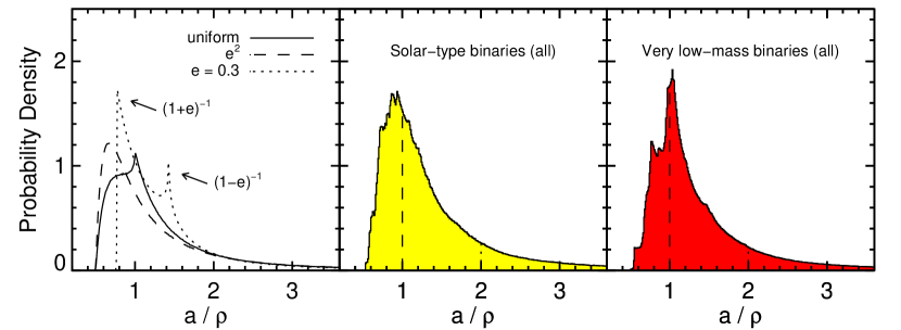
Figure 5: Distribution of conversion factors from projected separation ($\rho$) to true semimajor axis ($a$) for a variety of eccentricity distributions (see Table 6). The left panel shows the distribution at an arbitrary fixed eccentricity ($e=0.3$), as well as for two analytical eccentricity distributions: uniform and $e^{2}$ (Ambartsumian, 1937). For the solar-type binaries (middle) and very low-mass binaries (right), we show only the probability distributions for the full samples because subsets of these samples give essentially the same results. The dotted and dashed lines in the right two panels show where the distributions are truncated in the cases of moderate ($a/\rho=2$) and severe ($a/\rho=1$) discovery bias, respectively.

Table 1: New Keck AO Astrometry

Epoch (UT)	$\rho$ (mas)	PA (∘)	Filter	$\Delta{m}$ (mag)
LP 415-20AB (LGS)
2008 Jan 15	$89.3\pm 0.4$	$56.0\pm 0.5$ 0	$K_{S}$	$0.60\pm 0.07$
2008 Sep 08	$107.5\pm 0.8$0	$61.0\pm 0.3$ 0	$K_{S}$	$0.589\pm 0.013$
2009 Sep 28	$129.81\pm 0.15$0	$66.70\pm 0.06$0	$K_{S}$	$0.524\pm 0.022$
2010 Jan 09	$134.96\pm 0.19$0	$68.05\pm 0.05$0	$K_{S}$	$0.548\pm 0.016$
HD 130948BC (NGS)
2010 Jan 09	$89.0\pm 0.4$	$318.21\pm 0.25$00	$K_{S}$	$0.212\pm 0.023$
2010 Mar 22	$100.15\pm 0.15$0	$316.95\pm 0.07$00	$K$	$0.206\pm 0.007$

Table 2: Updated Orbit Determinations

Parameter	LP 415-20AB	HD 130948BC
$P$ (yr)	$14.4\pm 0.4$ 0	$10.28\pm 0.17$ 0
$a$ (mas)	$93.5^{+3.1}_{-2.3}$ 0	$124.5\pm 1.4$ 00
$e$	$0.708^{+0.016}_{-0.014}$0	$0.176\pm 0.006$
$i$ (∘)	$59.9\pm 2.2$ 0	$95.7\pm 0.2$ 0
$\Omega$ (∘)	$261.5^{+2.4}_{-2.7}$00	$313.39\pm 0.12$ 00
$\omega$ (∘)	$351\pm 7$ 00	$244\pm 3$ 0
$T_{0}$ (MJD)	$53505\pm 80$000	$54613\pm 22$ 000
$M_{\rm tot}$ ($M_{\sun}$)	$\cdots$	$0.1095\pm 0.0022$
$\chi^{2}$ (DOF)	6.83 (7)	9.38 (13)

Table 3: Visual Binaries with Published Orbits

Name	Sp. Type	Distance			Orbit				Orbit Quality			IWA	IWA/$a$
	Primary	$d$ (pc)	Ref.		$a$ (AU)	$e$	Ref.		$\Delta t_{\rm obs}/P$	$\sigma_{M}/M$		(″)
Gl 569Bab	M8.5	0$9.65\pm 0.16$	16		$0.923\pm 0.018$	$0.316\pm 0.005$	8		334%	$-$3%, +4%		0$\farcs$05	0.52
2MASS J0920$+$3517AB	T0	$25.4^{+0.8}_{-0.7}$	9		$1.67^{+0.06}_{-0.05}$	$0.217\pm 0.019$	9		144%	3%		0$\farcs$06	0.91
LP 349-25AB	M8	$13.2\pm 0.3$	10		$1.94\pm 0.04$	$0.051\pm 0.003$	8		76%	0.6%		0$\farcs$10	0.68
DENIS J2252$-$1730AB	L6	$15.0\pm 0.3$	9		$2.2^{+0.5}_{-0.2}$	$0.42^{+0.11}_{-0.08}$	9		34%–56%	5%		0$\farcs$07	0.48
HD 130948BC	L4	$18.17\pm 0.11$	16		$2.26\pm 0.03$	$0.176\pm 0.006$	1		73%	0.8%		0$\farcs$06	0.48
2MASS J2132$+$1341AB	L5	$27.5\pm 0.5$	9		$2.24\pm 0.10$	$0.34^{+0.03}_{-0.02}$	9		35%	5%		0$\farcs$05	0.61
$\epsilon$ Indi Bab	T1	0$3.624\pm 0.004$	16		$2.43\pm 0.11$	$0.53\pm 0.03$	2		38%	0.9%		0$\farcs$08	0.12
LP 415-20AB	M7.5	$[27\pm 4]$	1		$[2.5\pm 0.4]$	$0.708^{+0.016}_{-0.014}$	1		55%	$-$7%, +9%		0$\farcs$12	1.28
2MASS J0746$+$2000AB	L0	$12.21\pm 0.04$	5		$2.899\pm 0.013$	$0.487\pm 0.004$	1,11		68%	2%		0$\farcs$06	0.25
LHS 2397aAB	M8	$14.3\pm 0.4$	13		$3.09\pm 0.10$	$0.350\pm 0.005$	7		83%	3%		0$\farcs$12	0.56
2MASS J1534$-$2952AB	T5	$13.59\pm 0.22$	15		$3.2^{+0.4}_{-0.3}$	$0.10^{+0.09}_{-0.06}$	1,11		32%–44%	2%		0$\farcs$06	0.26
LHS 1070BC	M8.5	0$7.72\pm 0.15$	3		$3.56\pm 0.07$	$0.033^{+0.003}_{-0.002}$	1,14		82%	0.9%		0$\farcs$10	0.22
LHS 1901AB	M6.5	$12.9\pm 0.5$	12		$3.70\pm 0.16$	$0.194^{+0.025}_{-0.021}$	8		39%	1.4%		0$\farcs$10	0.35
2MASS J2140$+$1625AB	M8.5	$[26\pm 5]$	1		$[3.7\pm 0.7]$	$0.36^{+0.14}_{-0.10}$	1,11		38%–57%	$-$27%, +53%		0$\farcs$12	0.83
2MASS J0850$+$1057AB	L7	$38^{+7}_{-5}$	17		$4.8^{+3.9}_{-1.4}$	$0.64\pm 0.26$	11		10%–49%	100%		0$\farcs$06	0.48
2MASS J1728$+$3948AB	L5	$24.1^{+2.1}_{-1.8}$	17		$5.3\pm 0.8$	$0.28^{+0.35}_{-0.28}$	11		20%–47%	$-$27%, +167%		0$\farcs$06	0.27
2MASS J2206$-$2047AB	M8	$26.7^{+2.6}_{-2.1}$	4		$5.8^{+0.8}_{-0.7}$	$0.25\pm 0.08$	14		20%–28%	2.0%		0$\farcs$12	0.56
2MASS J1847$+$5522AB	M6.5	$[25\pm 5]$	1		$[5.8\pm 1.5]$	$0.1^{+0.5}_{-0.1}$	11		9%–23%	$-$72%, +194%		0$\farcs$08	0.34
2MASS J1750$+$4424AB	M7.5	$[29\pm 8]$	1		$[21\pm 13]$	$0.71\pm 0.18$	11		1.3%–9%	60%		0$\farcs$12	0.16
2MASS J1426$+$1557AB	M8.5	$[25\pm 5]$	1		$[60\pm 40]$	$0.85^{+0.10}_{-0.41}$	11		0.2%–20%	$-$100%, +73%		0$\farcs$12	0.05

Note. — This table includes all resolved binaries with a total mass $<0.2$ $M_{\sun}$ for which an orbit determination has been published. Orbit quality metrics are given for each binary: (1) fraction of orbital phase observed ($\Delta t_{\rm obs}/P$), if the period uncertainty is $>10\%$ the 1$\sigma$ range is given; and (2) fractional 1$\sigma$ error in the total mass from the orbit fit alone ($\sigma_{M}/M$), i.e., independent of the uncertainty in the distance. High quality orbits have a large fraction of the orbit covered and/or a low mass error.

References. — (1) This work; (2) Cardoso et al. (2009); (3) Costa et al. (2005); (4) Costa et al. (2006); (5) Dahn et al. (2002); (6) Dupuy et al. (2009a); (7) Dupuy et al. (2009c); (8) Dupuy et al. (2010); (9) Dupuy (2010); (11) Konopacky et al. (2010); (10) Gatewood & Coban (2009); (12) Lépine et al. (2009); (13) Monet et al. (1992); (14) Seifahrt et al. (2008); (15) Tinney et al. (2003). (16) van Leeuwen (2007); (17) Vrba et al. (2004).

Table 4: Very Low-Mass Binary Orbit Sample

Name	Int.-Light	Binary	$P$	$e$	$M_{\rm tot}$	Mass ratio	Orbit
	Sp. Type	Type	(days)		($M_{\sun}$)	($q\equiv M_{2}/M_{1}$)	Ref.
PPl 15	M6.5	S2	$5.8\pm 0.3$	$0.42\pm 0.05$	$[0.124\pm 0.004]$	$[0.85\pm 0.05]$	2
2MASS J0535$-$0546	M6.5	E	$9.77962\pm 0.00004$	$0.323\pm 0.006$	$0.088\pm 0.005$	$0.64\pm 0.04$	12
2MASS J0320$-$0446	M8	S1	$246.9\pm 0.5$ 00	$0.067\pm 0.015$	$[0.15\pm 0.03]$	[0.60–0.87]	3
LSR J1610$-$0040	d/sdM7	A,S1	$607\pm 4$ 00	$0.444\pm 0.017$	$[0.162\pm 0.015]$	[0.61–0.86]	5
Gl 569Bab	M8.5	V	$864.5\pm 1.1$ 00	$0.316\pm 0.005$	$0.140^{+0.009}_{-0.008}$	$[0.866^{+0.019}_{-0.014}]$	7
Cha H$\alpha$ 8	M5.75	S1	$1900\pm 130$ 0	$0.59\pm 0.22$	$[0.15\pm 0.02]$	[0.3–0.7]	9
LP 349-25AB	M8	V	$2834\pm 15$ 00	$0.051\pm 0.003$	$0.120^{+0.008}_{-0.007}$	$[0.872^{+0.014}_{-0.018}]$	7
HD 130948BC	L4	V	$3760\pm 60$ 00	$0.176\pm 0.006$	$0.1095\pm 0.0022$	$[0.948\pm 0.005]$	1
$\epsilon$ Indi Bab	T2.5	V	$4090\pm 180$ 0	$0.53\pm 0.03$	$0.116\pm 0.001$	$[0.63\pm 0.02]$	4
2MASS J2132$+$1341AB	L6	V	$4000^{+300}_{-200}$ 0	$0.34^{+0.03}_{-0.02}$	$[0.13\pm 0.02]$	$[0.76\pm 0.03]$	8
DENIS J2252$-$1730AB	L7.5	V	$4000^{+1500\phantom{0}}_{-700}$	$0.42^{+0.11}_{-0.08}$	$[0.12\pm 0.02]$	$[0.70\pm 0.03]$	8
2MASS J0746$+$2000AB	L0.5	V	$4640\pm 40$ 00	$0.487\pm 0.004$	$0.151\pm 0.003$	$[0.94\pm 0.02]$	1,10
LHS 2397aAB	M8	V	$5190\pm 40$ 00	$0.350\pm 0.005$	$0.146\pm 0.014$	$[0.71^{+0.09}_{-0.14}]$	6
LHS 1901AB	M7	V	$5880\pm 180$ 0	$0.830\pm 0.005$	$0.194^{+0.025}_{-0.021}$	$[0.958^{+0.015}_{-0.014}]$	7
LHS 1070BC	M8.5	V	$6220\pm 16$ 00	$0.033^{+0.003}_{-0.002}$	$0.156\pm 0.009$	$[0.84\pm 0.05]$	1,11
2MASS J1534$-$2952AB	T5	V	$8400^{+1500\phantom{0}}_{-1100}$	$0.10^{+0.09}_{-0.06}$	$0.061\pm 0.003$	$[0.936\pm 0.012]$	1,10

Note. — This table includes visual binaries from Table On the Distribution of Orbital Eccentricities for Very Low-Mass Binaries that pass our eccentricity de-biasing criteria ($0.9~{}{\rm AU}<a<3.7$ AU and IWA/$a<0.75$), as well as all unresolved binaries with a total mass $<0.2$ $M_{\sun}$ for which an orbit determination has been published. The type of each binary is given: astrometric (A), spectroscopic single-lined (S1) or double-lined (S2), eclipsing (E), or visual (V). All table values enclosed in brackets “[]” are estimates based on models. Mass ratio estimates for visual binaries are based on Lyon evolutionary models (Chabrier et al., 2000; Baraffe et al., 2003), while the estimates for the SB1s and SB2 are taken from the literature (Basri & Martín, 1999; Dahn et al., 2008; Burgasser & Blake, 2009; Joergens et al., 2010).

References. — (1) This work; (2) Basri & Martín (1999); (3) Blake et al. (2010); (4) Cardoso et al. (2009); (5) Dahn et al. (2008); (6) Dupuy et al. (2009c); (7) Dupuy et al. (2010); (8) Dupuy (2010); (9) Joergens et al. (2010); (10) Konopacky et al. (2010); (11) Seifahrt et al. (2008); (12) Stassun et al. (2006).

Table 5: Results of KS Tests

	Very Low-Mass Binaries
Comparison Sample	All		Visual only		$e<0.6$
	Prob.	$D$	Prob.	$D$	Prob.	$D$
Solar-type binaries ($P>\mbox{$P_{\rm circ}$}$)	0.50	$0.23\pm 0.04$	0.44	$0.28\pm 0.04$	0.57	$0.23\pm 0.04$
Solar-type binaries ($\mbox{$P_{\rm circ}$}<P<10^{3}$ days)	0.75	$0.22\pm 0.02$	0.82	$0.22\pm 0.04$	0.74	$0.23\pm 0.03$
Solar-type binaries ($P>10^{3}$ days)	0.25	$0.31\pm 0.05$	0.22	$0.36\pm 0.04$	0.46	$0.28\pm 0.03$
$e^{2}$ (Ambartsumian, 1937)	$9.1\times 10^{-5}$	$0.55\pm 0.04$	$2.2\times 10^{-3}$	$0.52\pm 0.04$	$5.3\times 10^{-7}$	$0.71\pm 0.03$
Bate (2009a)	0.83	$0.20\pm 0.04$	0.92	$0.19\pm 0.03$	0.64	$0.26\pm 0.04$
Bate (2009a, $a\leq 3.7$ AU)	0.95	$0.22\pm 0.04$	0.97	$0.22\pm 0.03$	0.91	$0.25\pm 0.05$
Stamatellos & Whitworth (2009)	$9.9\times 10^{-3}$	$0.59\pm 0.05$	0.034	$0.56\pm 0.05$	0.19	$0.52\pm 0.04$
Stamatellos & Whitworth (2009, $a\leq 3.7$ AU)	0.028	$0.56\pm 0.05$	0.064	$0.53\pm 0.05$	0.43	$0.45\pm 0.05$

Note. — Each table entry shows the probability that our sample of very low-mass orbits was drawn from the same parent distribution as the comparison sample along with the $D$ statistic and its rms scatter over $10^{4}$ Monte Carlo trials.

Table 6: Conversion Factors from Projected Separation to Semimajor Axis

Assumed $e$ Distribution	Correction factor ($a/\rho$)
	Median	68.3% c.l.	95.4% c.l.
No discovery bias
Uniform ($0<e<1$)	1.10	0.75, 2.02	0.57, 5.53
Circular ($e=0$)	1.15	1.01, 1.85	1.00, 4.72
$e^{2}$ (Ambartsumian, 1937)	1.02	0.67, 2.07	0.55, 6.00
Solar-type binaries ($P>\mbox{$P_{\rm circ}$}$)	1.15	0.81, 2.01	0.64, 5.11
Solar-type binaries ($\mbox{$P_{\rm circ}$}<P<10^{3}$ days)	1.16	0.83, 2.00	0.66, 5.04
Solar-type binaries ($P>10^{3}$ days)	1.14	0.78, 2.02	0.61, 5.29
Very low-mass (all binaries)	1.16	0.84, 1.97	0.66, 5.08
Very low-mass (visual binaries)	1.16	0.85, 1.97	0.66, 5.11
Moderate discovery bias (IWA = $a/2$)
Uniform ($0<e<1$)	1.02	0.72, 1.46	0.57, 1.89
Circular ($e=0$)	1.11	1.01, 1.46	1.00, 1.88
$e^{2}$ (Ambartsumian, 1937)	0.91	0.65, 1.42	0.55, 1.88
Solar-type binaries ($P>\mbox{$P_{\rm circ}$}$)	1.06	0.79, 1.51	0.63, 1.90
Solar-type binaries ($\mbox{$P_{\rm circ}$}<P<10^{3}$ days)	1.07	0.80, 1.51	0.65, 1.90
Solar-type binaries ($P>10^{3}$ days)	1.04	0.76, 1.50	0.60, 1.90
Very low-mass (all binaries)	1.08	0.82, 1.51	0.66, 1.90
Very low-mass (visual binaries)	1.08	0.82, 1.50	0.64, 1.90
Severe discovery bias (IWA = $a$)
Uniform ($0<e<1$)	0.79	0.63, 0.94	0.54, 0.99
$e^{2}$ (Ambartsumian, 1937)	0.74	0.61, 0.91	0.53, 0.99
Solar-type binaries ($P>\mbox{$P_{\rm circ}$}$)	0.83	0.70, 0.95	0.60, 0.99
Solar-type binaries ($\mbox{$P_{\rm circ}$}<P<10^{3}$ days)	0.84	0.71, 0.95	0.61, 0.99
Solar-type binaries ($P>10^{3}$ days)	0.82	0.68, 0.94	0.58, 0.99
Very low-mass (all binaries)	0.84	0.72, 0.96	0.58, 0.99
Very low-mass (visual binaries)	0.85	0.71, 0.96	0.58, 0.99

References

- Abt & Levy (1976) Abt, H. A., & Levy, S. G. 1976, ApJS, 30, 273
- Aitken (1918) Aitken, R. G. 1918, The binary stars, ed. Aitken, R. G.
- Allen (2007) Allen, P. R. 2007, ApJ, 668, 492
- Ambartsumian (1937) Ambartsumian, V. A. 1937, Astron. Zhurn., 14, 207
- Baraffe et al. (2003) Baraffe, I., Chabrier, G., Barman, T. S., Allard, F., & Hauschildt, P. H. 2003, A&A, 402, 701
- Basri & Martín (1999) Basri, G., & Martín, E. L. 1999, AJ, 118, 2460
- Bate (2009a) Bate, M. R. 2009a, MNRAS, 392, 590
- Bate (2009b) —. 2009b, MNRAS, 392, 1363
- Bate (2010) —. 2010, Highlights of Astronomy, 15, 769
- Berger et al. (2011) Berger, J., et al. 2011, A&A, 529, L1
- Blake et al. (2010) Blake, C. H., Charbonneau, D., & White, R. J. 2010, ApJ, 723, 684
- Blake et al. (2008) Blake, C. H., Charbonneau, D., White, R. J., Torres, G., Marley, M. S., & Saumon, D. 2008, ApJ, 678, L125
- Bouy et al. (2003) Bouy, H., Brandner, W., Martín, E. L., Delfosse, X., Allard, F., & Basri, G. 2003, AJ, 126, 1526
- Bouy et al. (2008) Bouy, H., et al. 2008, A&A, 481, 757
- Brown (2004) Brown, R. A. 2004, ApJ, 607, 1003
- Burgasser & Blake (2009) Burgasser, A. J., & Blake, C. H. 2009, AJ, 137, 4621
- Burgasser et al. (2006) Burgasser, A. J., Kirkpatrick, J. D., Cruz, K. L., Reid, I. N., Leggett, S. K., Liebert, J., Burrows, A., & Brown, M. E. 2006, ApJS, 166, 585
- Burgasser et al. (2003) Burgasser, A. J., Kirkpatrick, J. D., Reid, I. N., Brown, M. E., Miskey, C. L., & Gizis, J. E. 2003, ApJ, 586, 512
- Burgasser et al. (2008) Burgasser, A. J., Liu, M. C., Ireland, M. J., Cruz, K. L., & Dupuy, T. J. 2008, ApJ, 681, 579
- Burgasser et al. (2007) Burgasser, A. J., Reid, I. N., Siegler, N., Close, L., Allen, P., Lowrance, P., & Gizis, J. 2007, in Protostars and Planets V, ed. B. Reipurth, D. Jewitt, & K. Keil, 427–441
- Burke (2008) Burke, C. J. 2008, ApJ, 679, 1566
- Burrows et al. (2001) Burrows, A., Hubbard, W. B., Lunine, J. I., & Liebert, J. 2001, Reviews of Modern Physics, 73, 719
- Cardoso et al. (2009) Cardoso, C. V., et al. 2009, in American Institute of Physics Conference Series, Vol. 1094, American Institute of Physics Conference Series, ed. E. Stempels, 509–512
- Chabrier et al. (2000) Chabrier, G., Baraffe, I., Allard, F., & Hauschildt, P. 2000, ApJ, 542, 464
- Close et al. (2003) Close, L. M., Siegler, N., Freed, M., & Biller, B. 2003, ApJ, 587, 407
- Close et al. (2002) Close, L. M., Siegler, N., Potter, D., Brandner, W., & Liebert, J. 2002, ApJ, 567, L53
- Costa et al. (2005) Costa, E., Méndez, R. A., Jao, W.-C., Henry, T. J., Subasavage, J. P., Brown, M. A., Ianna, P. A., & Bartlett, J. 2005, AJ, 130, 337
- Costa et al. (2006) Costa, E., Méndez, R. A., Jao, W.-C., Henry, T. J., Subasavage, J. P., & Ianna, P. A. 2006, AJ, 132, 1234
- Cruz et al. (2007) Cruz, K. L., et al. 2007, AJ, 133, 439
- Dahn et al. (2008) Dahn, C. C., et al. 2008, ApJ, 686, 548
- Dahn et al. (2002) —. 2002, AJ, 124, 1170
- Dupuy (2010) Dupuy, T. J. 2010, PhD thesis, University of Hawai’i at Manoa
- Dupuy et al. (2009a) Dupuy, T. J., Liu, M. C., & Bowler, B. P. 2009a, ApJ, 706, 328
- Dupuy et al. (2010) Dupuy, T. J., Liu, M. C., Bowler, B. P., & Cushing, M. C. 2010, ApJ, 721, 1725
- Dupuy et al. (2009b) Dupuy, T. J., Liu, M. C., & Ireland, M. J. 2009b, ApJ, 692, 729
- Dupuy et al. (2009c) —. 2009c, ApJ, 699, 168
- Duquennoy & Mayor (1991) Duquennoy, A., & Mayor, M. 1991, A&A, 248, 485
- Fischer & Marcy (1992) Fischer, D. A., & Marcy, G. W. 1992, ApJ, 396, 178
- Gatewood & Coban (2009) Gatewood, G., & Coban, L. 2009, AJ, 137, 402
- Ghez et al. (2008) Ghez, A. M., et al. 2008, ApJ, 689, 1044
- Gizis et al. (2000) Gizis, J. E., Monet, D. G., Reid, I. N., Kirkpatrick, J. D., Liebert, J., & Williams, R. J. 2000, AJ, 120, 1085
- Harrington & Miranian (1977) Harrington, R. S., & Miranian, M. 1977, PASP, 89, 400
- Joergens & Müller (2007) Joergens, V., & Müller, A. 2007, ApJ, 666, L113
- Joergens et al. (2010) Joergens, V., Müller, A., & Reffert, S. 2010, A&A, 521, A24
- Kirkpatrick et al. (2000) Kirkpatrick, J. D., et al. 2000, AJ, 120, 447
- Konopacky et al. (2010) Konopacky, Q. M., Ghez, A. M., Barman, T. S., Rice, E. L., Bailey, J. I., White, R. J., McLean, I. S., & Duchêne, G. 2010, ApJ, 711, 1087
- Kraus & Hillenbrand (2009) Kraus, A. L., & Hillenbrand, L. A. 2009, ApJ, 703, 1511
- Lépine et al. (2009) Lépine, S., Thorstensen, J. R., Shara, M. M., & Rich, R. M. 2009, AJ, 137, 4109
- Liu et al. (2008) Liu, M. C., Dupuy, T. J., & Ireland, M. J. 2008, ApJ, 689, 436
- Liu et al. (2010) Liu, M. C., Dupuy, T. J., & Leggett, S. K. 2010, ApJ, 722, 311
- Mathieu (1994) Mathieu, R. D. 1994, ARA&A, 32, 465
- Monet et al. (1992) Monet, D. G., Dahn, C. C., Vrba, F. J., Harris, H. C., Pier, J. R., Luginbuhl, C. B., & Ables, H. D. 1992, AJ, 103, 638
- Pourbaix et al. (2004) Pourbaix, D., et al. 2004, A&A, 424, 727
- Raghavan et al. (2010) Raghavan, D., et al. 2010, ApJS, 190, 1
- Reid et al. (2001) Reid, I. N., Gizis, J. E., Kirkpatrick, J. D., & Koerner, D. W. 2001, AJ, 121, 489
- Reid et al. (2006) Reid, I. N., Lewitus, E., Allen, P. R., Cruz, K. L., & Burgasser, A. J. 2006, AJ, 132, 891
- Reipurth & Clarke (2001) Reipurth, B., & Clarke, C. 2001, AJ, 122, 432
- Reipurth et al. (2007) Reipurth, B., Guimarães, M. M., Connelley, M. S., & Bally, J. 2007, AJ, 134, 2272
- Rice et al. (2003) Rice, W. K. M., Armitage, P. J., Bonnell, I. A., Bate, M. R., Jeffers, S. V., & Vine, S. G. 2003, MNRAS, 346, L36
- Schaefer et al. (2006) Schaefer, G. H., Simon, M., Beck, T. L., Nelan, E., & Prato, L. 2006, AJ, 132, 2618
- Seifahrt et al. (2008) Seifahrt, A., Röll, T., Neuhäuser, R., Reiners, A., Kerber, F., Käufl, H. U., Siebenmorgen, R., & Smette, A. 2008, A&A, 484, 429
- Shen & Turner (2008) Shen, Y., & Turner, E. L. 2008, ApJ, 685, 553
- Siegler et al. (2007) Siegler, N., Close, L. M., Burgasser, A. J., Cruz, K. L., Marois, C., Macintosh, B., & Barman, T. 2007, AJ, 133, 2320
- Siegler et al. (2003) Siegler, N., Close, L. M., Mamajek, E. E., & Freed, M. 2003, ApJ, 598, 1265
- Stamatellos et al. (2007) Stamatellos, D., Hubber, D. A., & Whitworth, A. P. 2007, MNRAS, 382, L30